Status of neutrino oscillations I:
the three-neutrino scenario

Abstract:

We present a global analysis of neutrino oscillation data within the three-neutrino oscillation scheme, including in our fit all the current solar neutrino data, the reactor neutrino data from KamLAND and CHOOZ, the atmospheric neutrino data from Super-Kamiokande and MACRO, and the first data from the K2K long-baseline accelerator experiment. We determine the current best fit values and allowed ranges for the three-flavor oscillation parameters, discussing the relevance of each individual data set as well as the complementarity of different data sets. Furthermore, we analyze in detail the status of the small parameters $\theta_{13}$ and $\Delta m^{2}_{21}/\Delta m^{2}_{31}$, which fix the possible strength of CP violating effects in neutrino oscillations.

1 Introduction

Recently, the Sudbury Neutrino Observatory (SNO) experiment [1] has released an improved measurement with enhanced neutral current sensitivity due to neutron capture on salt, which has been added to the heavy water in the SNO detector. This adds precious information to the large amount of data on neutrino oscillations published in the last few years. Thanks to this growing body of data a rather clear picture of the neutrino sector is starting to emerge. In particular, the results of the KamLAND reactor experiment [2] have played an important role in confirming that the disappearance of solar electron neutrinos [3, 4, 5, 6, 7], the long-standing solar neutrino problem, is mainly due to oscillations and not to other types of neutrino conversions. Moreover, KamLAND has pinned down that the oscillation solution to the solar neutrino problem is the large mixing angle MSW solution (LMA) [8, 9, 10, 11] characterized by the presence of matter effects [12, 13]. On the other hand, experiments with atmospheric neutrinos [14, 15, 16] show strong evidence in favor of $\nu_{\mu}\to\nu_{\tau}$ oscillations, in agreement with the first data from the K2K accelerator experiment [17]. Together with the non-observation of oscillations in reactor experiments at a baseline of about 1 km [18, 19], and the strong rejection against transitions involving sterile states [20], these positive evidences can be very naturally accounted for within a three-neutrino framework. The large and nearly maximal mixing angles indicated by the solar and atmospheric neutrino data samples, respectively, come as a surprise for particle physicists, as it contrasts with the small angles characterizing the quark sector.

In this talk we present a complete analysis of all the available neutrino data in the context of the three-neutrino oscillation scenario. As a first step, in Sec. 2 we discuss each individual data set (solar, atmospheric, CHOOZ, KamLAND and K2K) in a simplified two-neutrino approach. Then, in Sec. 3 we discuss the general three-neutrino case, focusing on the complementarity of different data sets and and deriving the allowed ranges for all the oscillation parameters. Furthermore, we discuss in detail the constraints on the small parameters $\theta_{13}$ and the ratio $\Delta m^{2}_{21}/\Delta m^{2}_{31}$, which are the crucial quantities governing the possible strength of CP violating effects in neutrino oscillations. In Sec. 4 we summarize our results.

2 Two-neutrino analysis

2.1 Solar neutrino data

In order to determine the values of neutrino masses and mixing for the oscillation solution of the solar neutrino problem, we have taken into account the most recent results from all the solar neutrino experiments. This includes the rate of the chlorine experiment at the Homestake mine [3] ($2.56\pm 0.16\pm 0.16$ SNU), the latest results [21] of the gallium experiments SAGE [4] ($69.1~{}^{+4.3}_{-4.2}~{}^{+3.8}_{-3.4}$ SNU) and GALLEX/GNO [5] ($69.3\pm 4.1\pm 3.6$), the 1496-day Super-Kamiokande data sample [6] in the form of 44 bins (8 energy bins, 6 of which are further divided into 7 zenith angle bins), the SNO-I neutral current, spectral and day/night data [7] divided into 34 bins (17 energy bins for each day and night period), and the very recent SNO-II measurement of charged current (CC), neutral current (NC) and elastic scattering (ES) interaction rates with enhanced neutral current sensitivity due to neutron capture on salt. Therefore, in our statistical analysis we use $3+44+34+3=84$ observables, which we fit in terms of the two parameters $\Delta m^{2}_{\text{sol}}$ and $\theta_{\text{sol}}$. The analysis methods used here are similar to the ones described in Refs. [20, 22] and references therein, with the exception that in the current work we use the so-called pull-approach for the $\chi^{2}$ calculation. As described in Ref. [23], each systematic uncertainty is included by introducing a new parameter in the fit and adding a penalty function to the $\chi^{2}$. However, the method described in Ref. [23] is extended in two respects. First, it is generalized to the case of correlated statistical errors [24], as necessary to treat the SNO-salt data. Second, in the calculation of the total $\chi^{2}$ we use the exact relation between the theoretical predictions and the pulls associated to the solar neutrino fluxes, rather than keeping only the terms up to first order. This is particularly relevant for the case of the solar ⁸B flux, which is constrained by the new SNO data with an accuracy better than the prediction of the Standard Solar Model (SSM) [25]. In our approach it is possible to take into account on the same footing both the SSM boron flux prediction and the SNO NC measurement, without pre-selecting one particular value. In this way the fit itself can choose the best compromise between the SNO NC data and the SSM value.

In Fig. 1(a) we show the allowed regions and the $\Delta\chi^{2}$ functions from the analysis of all solar neutrino experiments, including the new SNO-salt data. One finds that especially the upper part of the LMA region and large mixing angles are now strongly constrained [26]. This follows mainly from the rather small measured value of the CC/NC ratio of $0.306\pm 0.026\pm 0.024$ [1], since this observable increases when moving to larger values of $\Delta m^{2}_{\text{sol}}$ and/or $\sin^{2}\theta_{\text{sol}}$ (see, e.g., Ref. [11]). In is worth noting that the LOW solution is now excluded at more than $3\sigma$, and the quasi-vacuum region at more than $5\sigma$, even without the inclusion of KamLAND. The best fit values for the oscillation parameters are

$$\sin^{2}\theta_{\text{sol}}=0.29\,,\qquad\Delta m^{2}_{\text{sol}}=6.0\times 10^{-5}~{}\text{eV}^{2}\qquad\text{(solar data)}.$$ (1)

The new SNO-salt data strongly enhances the rejection against maximal solar mixing: from the $\Delta\chi^{2}$ projected onto the $\sin^{2}\theta_{\text{sol}}$ axis, shown in Fig. 1(a), we find that $\theta_{\text{sol}}=45^{\circ}$ is excluded at more than $5\sigma$, ruling out all bi-maximal models of neutrino masses.

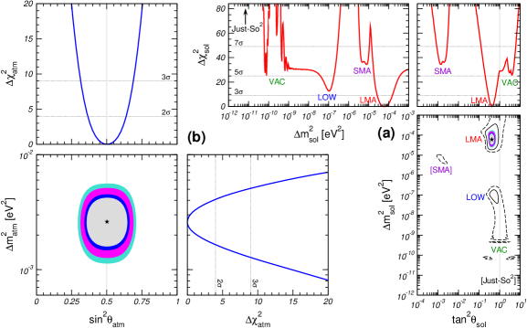
Figure 1: Allowed regions at 90%, 95%, 99%, and $3\sigma$ C.L. (2 d.o.f.) from the analysis of solar neutrino data (a) and of atmospheric neutrino data (b), in the two-neutrino oscillation approximation. In the solar plane (a) we also show the $5\sigma$ (solid line) and $7\sigma$ (dashed line) allowed regions. Also displayed is $\Delta\chi^{2}$ as a function of the relevant oscillation parameters.

2.2 Atmospheric neutrino data

For the atmospheric data analysis we use all the charged-current data from the Super-Kamiokande [15] and MACRO [16] experiments. The Super-Kamiokande data include the $e$-like and $\mu$-like data samples of sub- and multi-GeV contained events (10 bins in zenith angle), as well as the stopping (5 angular bins) and through-going (10 angular bins) up-going muon data events. As previously, we do not use the information on $\nu_{\tau}$ appearance, multi-ring $\mu$ and neutral-current events since an efficient Monte-Carlo simulation of these data sample would require a more detailed knowledge of the Super Kamiokande experiment, and in particular of the way the neutral-current signal is extracted from the data. Such an information is presently not available to us. From MACRO we use the through-going muon sample divided in 10 angular bins [16]. We did not include in our fit the results of other atmospheric neutrino experiments since at the moment the statistics is completely dominated by Super-Kamiokande.

Our statistical analysis of the atmospheric data described in Ref. [20, 22]. In particular, we now take advantage of the full ten-bin zenith-angle distribution for the contained events, rather than the five-bin distribution employed in our older publications. Therefore, we have now $65$ observables, which we fit in terms of the two relevant parameters $\Delta m^{2}_{\text{atm}}$ and $\theta_{\text{atm}}$. Concerning the theoretical Monte-Carlo, we improved the method presented in Ref. [22] by properly taking into account the scattering angle between the incoming neutrino and the scattered lepton directions. This was already the case for Sub-GeV contained events, however previously we made the simplifying assumption of full neutrino-lepton collinearity in the calculation of the expected event numbers for the Multi-GeV contained and up-going-$\mu$ data samples. While this approximation is still justified for the stopping and through-going muon samples, in the Multi-GeV sample the theoretically predicted value for down-coming $\nu_{\mu}$ is systematically higher if full collinearity is assumed. The reason for this is that the strong suppression observed in these bins cannot be completely ascribed to the oscillation of the down-coming neutrinos (which is small due to small travel distance). Because of the non-negligible neutrino-lepton scattering angle at these Multi-GeV energies there is a sizable contribution from up-going neutrinos (with a higher conversion probability due to the longer travel distance) to the down-coming leptons. However, this problem is less visible when the angular information of Multi-GeV events is included in a five angular bins presentation of the data, as previously assumed.

We note that recently the Super-Kamiokande collaboration has presented a preliminary reanalysis of their atmospheric data [27]. The update includes changes in the detector simulation, data analysis and input atmospheric neutrino fluxes. These changes lead to a slight downward shift of the mass-splitting to the best fit value of $\Delta m^{2}_{\text{atm}}=2\times 10^{-3}~{}\text{eV}^{2}$. Currently it is not possible to recover enough information from Ref. [27] to incorporate the corresponding changes in our codes. We note, however, that the quoted value for $\Delta m^{2}_{\text{atm}}$ is statistically compatible with our result. For $\Delta m^{2}_{\text{atm}}=2\times 10^{-3}~{}\text{eV}^{2}$ and maximal mixing we obtain a $\Delta\chi^{2}=1.3$.

In Fig. 1(b) we summarize our results for the analysis of atmospheric neutrino experiments. First of all, we note that the dependence of the atmospheric $\Delta\chi^{2}$ over the oscillation parameters $\Delta m^{2}_{\text{atm}}$ and $\theta_{\text{atm}}$ exhibits a beautiful quadratic behavior, reflecting the fact that the oscillation solution to the atmospheric neutrino problem is robust and unique. The best fit values and the $3\sigma$ ranges (1 d.o.f.) for the oscillation parameters are:

$$\sin^{2}\theta_{\text{atm}} =0.5\,, 0.3\leq\sin^{2}\theta_{\text{atm}} \leq 0.7\,,$$ (2)

$$\Delta m^{2}_{\text{atm}} =2.5\times 10^{-3}~{}\text{eV}^{2}\,, 1.2\times 10^{-3}~{}\text{eV}^{2}\leq\Delta m^{2}_{\text{atm}} \leq 4.8\times 10^{-3}~{}\text{eV}^{2}\,.$$ (3)

Note that in the two-neutrino approximation the neutrino conversion occur completely in the channel $\nu_{\mu}\to\nu_{\tau}$, and in this case the contour regions are symmetric under the transformation $\theta_{\text{atm}}\to\pi/4-\theta_{\text{atm}}$ due to the cancellation of matter effects.

2.3 CHOOZ

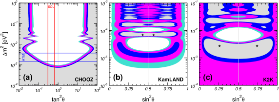
Figure 2: Allowed regions at 90%, 95%, 99%, and $3\sigma$ C.L. (2 d.o.f.) from the analysis of CHOOZ (a), KamLAND (b), and K2K data (c).

The CHOOZ experiment [18] searches for disappearance of $\bar{\nu}_{e}$ produced in a power station with two pressurized-water nuclear reactors with a total thermal power of $8.5$ GW (thermal). At the detector, located at $L\simeq 1$ Km from the reactors, the $\bar{\nu}_{e}$ reaction signature is the delayed coincidence between the prompt ${\rm e^{+}}$ signal and the signal due to the neutron capture in the Gd-loaded scintillator. Since no evidence was found for a deficit of measured vs. expected neutrino interactions, the result of this experiment is a bound on the oscillation parameters describing the mixing of $\nu_{e}$ with all the other neutrino species. In the two-neutrino limit the only relevant parameters to describe the oscillations are a mass-squared splitting $\Delta m^{2}$ and a mixing angle $\theta$, and in Fig. 2(a) we show the exclusion plot in this plane. From this figure we see that at the $3\sigma$ level the region $\Delta m^{2}\gtrsim 10^{-3}~{}\text{eV}^{2}$ and $0.05\lesssim\tan^{2}\theta\lesssim 20$ is excluded.

The result of this experiment, once combined with solar and atmospheric data, has important implications for the determination of the oscillations parameters. This can be qualitatively understood even without performing a detailed three-neutrino analysis. For what concerns solar data, since solar neutrino conversion occur in the channel $\nu_{e}\to\nu_{a}$, which is the same channel measured by CHOOZ once the CPT symmetry is assumed, the constraints imposed by CHOOZ on the solar parameters can be immediately derived from Fig. 2(a) by identifying $\Delta m^{2}$ and $\theta$ with $\Delta m^{2}_{\text{sol}}$ and $\theta_{\text{sol}}$, respectively. The two vertical red lines in Fig. 2(a) delimit the $3\sigma$ allowed region for $\theta_{\text{sol}}$, as found in Sec. 2.1, and it is straightforward to see that values of $\Delta m^{2}_{\text{sol}}\gtrsim 10^{-3}~{}\text{eV}^{2}$ are incompatible with the CHOOZ result. Therefore, CHOOZ implies an upper bound on $\Delta m^{2}_{\text{sol}}$. This result was particularly relevant before the release of the SNO data on neutral-current interactions, since at that time the CHOOZ bound was the only measurement providing a solid upper bound on $\Delta m^{2}_{\text{sol}}$.

Concerning atmospheric data, the implications of the CHOOZ result require a more complete formalism. In the next section we will see that, in the three-neutrino scenario, the mixing of the electron neutrino with the $\nu_{\mu}-\nu_{\tau}$ admixture responsible for atmospheric conversion is described by a mixing angle which we will denote by $\theta_{13}$. Therefore, the two-dimensional exclusion plot shown if Fig. 2(a) can also be interpreted as a constraint in the plane $(\Delta m^{2}_{\text{atm}},\,\theta_{13})$. The two horizontal blue lines in this figure delimit the $3\sigma$ allowed region in $\Delta m^{2}_{\text{atm}}$, as found in Sec. 2.2, and we can see that the CHOOZ measurement implies that $\theta_{13}$ must be small. This means that the electron neutrino is essentially decoupled from atmospheric neutrino oscillations, thus justifying a posteriori the use of the two-neutrino approximation for the analysis of atmospheric data.

2.4 KamLAND

The KamLAND experiment is a reactor neutrino experiment with its detector located at the Kamiokande site. Most of the $\bar{\nu}_{e}$ flux incident at KamLAND comes from plants at distances of $80-350$ km from the detector, making the average baseline of about 180 kilometers, long enough to provide a sensitive probe of the LMA solution of the solar neutrino problem. In KamLAND the target for the $\bar{\nu}_{e}$ flux consists of a spherical transparent balloon filled with 1000 tons of non-doped liquid scintillator, and the anti-neutrinos are detected via the inverse neutron $\beta$-decay $\bar{\nu}_{e}+p\to e^{+}+n$.

The KamLAND collaboration has for the first time measured the disappearance of neutrinos traveling to a detector from a power reactor. They observe a strong evidence for the disappearance of electron anti-neutrinos during their flight, giving the first terrestrial confirmation of the solar neutrino anomaly and also establishing the oscillation hypothesis with man-produced neutrinos. Moreover, the parameters that describe this disappearance of the electron neutrino in terms of oscillations are perfectly consistent with latest determinations of solar neutrino parameters in a CPT-conserving scenario.

The details of the statistical analysis of the KamLAND data can be found in Ref. [28]. Instead of the usual $\chi^{2}$-fit analysis based on energy binned data, we use an event-by-event likelihood approach which gives stronger constraints. The results of our analysis are summarized in Fig. 2(b), where we show the allowed regions of the oscillation parameters. It is in good agreement with the analysis performed by the KamLAND group, shown in Fig. 6 of Ref. [2]. This gives us confidence on our simulation of the KamLAND data and therefore encourages us to use it in a full analysis combining also with the other data samples.

2.5 K2K

The last data set which we include in our fits is the KEK to Kamioka long-baseline neutrino oscillation experiment (K2K) [17]. The neutrino beam used by this experiment is composed by muon neutrinos at 98%, and has a mean energy of 1.3 GeV. Since the neutrino flight distance is approximately 250 km, K2K can provide a sensitive proves of atmospheric oscillations. In our analysis we use the 29 single-ring muon events, grouped into 6 energy bins, and we perform a spectral analysis similar to the one described in Ref. [29]. Our results are summarized in Fig. 2(c).

3 Global three-neutrino analysis

3.1 Notation

In general, the determination of the oscillation probabilities requires the solution of the Schrödinger evolution equation of the neutrino system in the Sun- and/or Earth-matter background [10, 22, 30]:

$$i\frac{d\vec{\nu}}{dt}={\bf H}\,\vec{\nu},\qquad{\bf H}={\bf U}\cdot{\bf H}_{0}^{d}\cdot{\bf U}^{\dagger}+{\bf V},$$ (4)

where ${\bf U}$ is the unitary matrix connecting the flavor basis and the mass basis in vacuum, ${\bf H}_{0}^{d}$ is the vacuum Hamiltonian and V describes charged-current forward interactions in matter. For a CP-conserving three-flavor scenario, we have:

$${\bf H}_{0}^{d} =\frac{1}{2E_{\nu}}\,{\bf diag}\left(-\Delta m^{2}_{21},\,0,\,\Delta m^{2}_{32}\right);$$ (5)

$${\bf U} ={\bf U}_{23}(\theta_{23})\cdot{\bf U}_{13}(\theta_{13})\cdot{\bf U}_{12}(\theta_{12})\,;$$

$${\bf V} =\pm\sqrt{2}G_{F}\,{\bf diag}\left(N_{e},\,0,\,0\right);$$

$$\vec{\nu} =\left(\nu_{e},\,\nu_{\mu},\,\nu_{\tau}\right).$$

In the general case, the three-neutrino transition probabilities depend on five parameters, namely the two mass-squared differences $\Delta m^{2}_{21}$, $\Delta m^{2}_{31}$ and the three mixing angles $\theta_{12}$, $\theta_{13}$, $\theta_{23}$. However, from the two-neutrino analysis presented in the previous section we see that, in order to accommodate both solar and atmospheric neutrino data into a unified framework, an hierarchy between the two mass-squared differences is required:

$$\left(\Delta m^{2}_{\text{sol}}\equiv\Delta m^{2}_{21}\right)\ll\left(\Delta m^{2}_{\text{atm}}\equiv\Delta m^{2}_{31}\approx\Delta m^{2}_{32}\right).$$ (6)

Both for the solar and the atmospheric neutrino data analysis we can take advantage of this hierarchy to reduce the number of parameters [31]. This implies first of all that the effect of a possible Dirac CP-violating phase in the lepton mixing matrix can be neglected. Also, for what concerns the solar case we can set $\Delta m^{2}_{31}\approx\infty$ and also disregard the atmospheric angle $\theta_{23}$, since it never appears in the relevant transition probabilities. Conversely, for the atmospheric case we can set $\Delta m^{2}_{21}\approx 0$ and in this limit the solar angle $\theta_{12}$ cancels out from the equations. So in both the cases we are left with only three parameters, among which only the reactor angle $\theta_{13}$ is common to both the problems. We will further comment on the goodness of the hierarchy approximation at the end of the next section.

3.2 Discussion

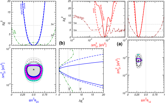
Figure 3: Allowed regions at 90%, 95%, 99%, and $3\sigma$ C.L. (2 d.o.f.) from the analysis of solar (hollow regions) and solar+KamLAND (colored regions) neutrino data (a), and of atmospheric (hollow regions) and atmospheric+K2K (colored regions) neutrino data (b), in terms of three-neutrino oscillation parameters. In both analyses we set $\theta_{13}=0$. Also displayed is $\Delta\chi^{2}$ as a function of the relevant oscillation parameters.

Having discussed each independent data set separately, we now turn our attention to the bound on neutrino oscillation parameters coming from combinations of different data sets. The results of our analysis are summarized in Figs. 3 and 4. In Figs. 3(a) and 3(b) we show the projections on the planes $(\Delta m^{2}_{21},\,\theta_{12})$ and $(\Delta m^{2}_{31},\,\theta_{23})$ of the combination of solar+KamLAND data and atmospheric+K2K data, respectively, for $\theta_{13}=0$. In Fig. 4 we show the allowed regions and the $\Delta\chi^{2}$ function from the analysis of all neutrino data.

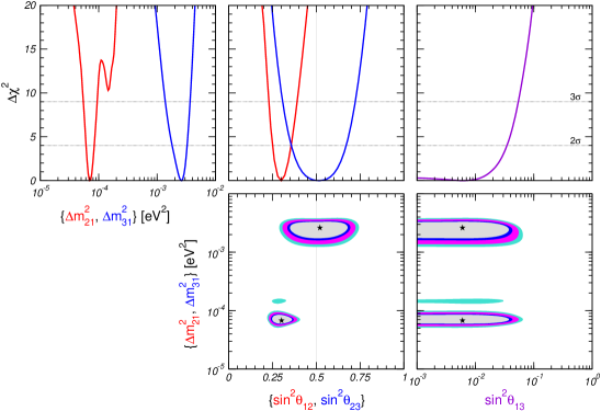
Figure 4: Projections of the allowed regions from the global oscillation data at 90%, 95%, 99%, and $3\sigma$ C.L. for 2 d.o.f. for various parameter combinations. Also shown is $\Delta\chi^{2}$ as a function of the oscillation parameters $\theta_{12}$, $\theta_{23}$, $\theta_{13}$, $\Delta m^{2}_{21}$ and $\Delta m^{2}_{31}$, minimized with respect to all undisplayed parameters.

From Figs. 3(a) and 3(b), we see that the inclusion of KamLAND and K2K data drastically improves the determination of the two mass-squared differences $\Delta m^{2}_{21}$ and $\Delta m^{2}_{31}$. In particular, K2K is responsible for the strong improvement of the upper bound on $\Delta m^{2}_{31}$, leaving the lower bound essentially unaffected. On the other hand, the recent KamLAND result single out LMA as the only viable oscillation solution to the solar neutrino problem. As noted in Ref. [8], the original LMA region is split by KamLAND into two separate islands, called LMA-I (characterized by $\Delta m^{2}_{21}\approx 7\times 10^{-5}~{}\text{eV}^{2}$) and LMA-II (with $\Delta m^{2}_{21}\approx 1.5\times 10^{-4}~{}\text{eV}^{2}$). The inclusion of the recent SNO-salt data practically rules out the LMA-II solution, which is now disfavored with a $\Delta\chi^{2}=10.3$ with respect to LMA-I [26]. The best-fit point and the $3\sigma$ ranges for the global analysis (see Fig. 4) are:

$$\Delta m^{2}_{21} =6.9\times 10^{-5}~{}\text{eV}^{2}\,, 5.4\times 10^{-5}~{}\text{eV}^{2}\leq\Delta m^{2}_{21} \leq 9.5\times 10^{-5}~{}\text{eV}^{2}\,,$$ (7)

$$\Delta m^{2}_{31} =2.6\times 10^{-3}~{}\text{eV}^{2}\,, 1.4\times 10^{-3}~{}\text{eV}^{2}\leq\Delta m^{2}_{31} \leq 3.7\times 10^{-3}~{}\text{eV}^{2}\,.$$ (8)

The determination of the oscillation angles $\theta_{12}$ and $\theta_{23}$ is dominated by solar and atmospheric data, respectively, while reactor and accelerator experiments only play a marginal role in this respect. As discussed in Sec. 2.1, the recent SNO-salt data drastically improves the upper bound on the solar angle $\theta_{12}$, and maximal mixing $\theta_{12}=45^{\circ}$ is now ruled out at more than $5\sigma$. Conversely, atmospheric data clearly prefer $\theta_{23}=45^{\circ}$. From the global analysis, we have that best-fit point and the $3\sigma$ ranges are:

$$\sin^{2}\theta_{12} =0.3\,, 0.23\leq\sin^{2}\theta_{12} \leq 0.39\,,$$ (9)

$$\sin^{2}\theta_{23} =0.52\,, 0.36\leq\sin^{2}\theta_{23} \leq 0.67\,.$$ (10)

Note that the small deviation from maximal mixing of $\theta_{23}$ is due to the fact that the data prefer a small but non-vanishing value of $\theta_{13}$, which breaks the invariance under the transformation $\theta_{23}\to\pi/2-\theta_{23}$. However, currently this effect has no statistical significance at all.

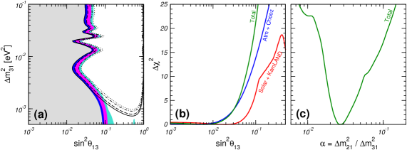
Figure 5: (a) Allowed regions in the $(\sin^{2}\theta_{13},\,\Delta m^{2}_{31})$ plane at 90%, 95%, 99%, and $3\sigma$ from CHOOZ data alone (lines) and CHOOZ+solar+KamLAND data (colored regions). (b) $\Delta\chi^{2}$ profiles projected onto the $\sin^{2}\theta_{13}$ axis, for solar+KamLAND, atmospheric+CHOOZ, and for global data. (c) $\Delta\chi^{2}$ from global oscillation data as a function of $\alpha\equiv\Delta m^{2}_{21}/\Delta m^{2}_{31}$.

The last angle in the three-neutrino mixing matrix, $\theta_{13}$, is presently still unknown. At the moment only an upper bound exists, which is mainly dominated by the CHOOZ reactor experiment [18]. In Fig. 5(b) we show the $\Delta\chi^{2}$ as a function of $\sin^{2}\theta_{13}$ for different data sample choices. One can see how the bound on $\sin^{2}\theta_{13}$ as implied by the CHOOZ experiment in combination with the atmospheric neutrino data still provides the main restriction on $\sin^{2}\theta_{13}$. We find the following bounds at 90% C.L. ($3\sigma$) for 1 d.o.f.:

$$\sin^{2}\theta_{13}\leq\left\{\begin{array}[]{l@{\qquad}l}0.070~{}(0.12)&\text{(solar+KamLAND)}\\ 0.028~{}(0.066)&\text{(CHOOZ+atmospheric)}\\ 0.029~{}(0.054)&\text{(global data)}\end{array}\right.$$ (11)

However, we note that the solar data contributes in an important way to the constraint on $\sin^{2}\theta_{13}$ for lower values of $\Delta m^{2}_{31}$. In particular, the downward shift of $\Delta m^{2}_{31}$ reported in Ref. [27] implies a significant loosening of the CHOOZ bound on $\sin^{2}\theta_{13}$, since this bound gets quickly weak when $\Delta m^{2}_{31}$ decreases (see, e.g., Ref. [32]). Such loosening in sensitivity is prevented to some extent by solar neutrino data. In Fig. 5(a) we show the allowed regions in the $(\sin^{2}\theta_{13},\,\Delta m^{2}_{31})$ plane from an analysis including solar and reactor neutrino data (CHOOZ and KamLAND). One finds that, although for larger $\Delta m^{2}_{31}$ values the bound on $\sin^{2}\theta_{13}$ is dominated by the CHOOZ + atmospheric data, for low $\Delta m^{2}_{31}\simeq 10^{-3}~{}\text{eV}^{2}$ the solar + KamLAND bound is comparable to that coming from CHOOZ + atmospheric. For example, fixing $\Delta m^{2}_{31}=2\times 10^{-3}~{}\text{eV}^{2}$ we obtain at 90% C.L. ($3\sigma$) for 1 d.o.f. the bound

$$\sin^{2}\theta_{13}\leq 0.035~{}(0.066)\qquad(\Delta m^{2}_{31}=2\times 10^{-3}~{}\text{eV}^{2})\,,$$ (12)

which is slightly worse than the bound from global data shown in Eq. (11).

For the exploration of genuine three-flavor effects such as CP-violation the mass hierarchy parameter $\alpha\equiv\Delta m^{2}_{21}/\Delta m^{2}_{31}$ is of crucial importance since, in a three-neutrino scheme, CP violation disappears in the limit where two neutrinos become degenerate. Therefore we show in Fig. 5(c) the $\Delta\chi^{2}$ from the global data as a function of this parameter. We obtain the following best fit values and $3\sigma$ intervals:

$$\begin{split}\alpha=0.026\,,\qquad 0.018\leq\alpha\leq 0.053.\end{split}$$ (13)

Note that the strong upper bound found on $\alpha$ justifies a posteriori the use of the hierarchy approximation in the calculation of solar and atmospheric $\chi^{2}$ functions [31].

4 Conclusions

In this talk we have presented a global analysis of neutrino oscillation data in the three-neutrino scheme, including in our fit all the current solar neutrino data, the reactor neutrino data from KamLAND and CHOOZ, the atmospheric neutrino data from Super-Kamiokande and MACRO, and the first data from the K2K long-baseline accelerator experiment. We have discussed the implications of each individual data set, as well as the complementarity of different data sets, on the determination of the neutrino oscillation parameters, and we have determined the current best fit values and allowed ranges for the three-flavor oscillation parameters $\theta_{12}$, $\theta_{23}$, $\theta_{13}$, $\Delta m^{2}_{21}$, $\Delta m^{2}_{31}$. Furthermore, we have analyzed in detail the limits on the small mixing angle $\sin^{2}\theta_{13}$ and on the hierarchy parameter $\alpha=\Delta m^{2}_{21}/\Delta m^{2}_{31}$. These small parameters are relevant for genuine three flavor effects, and restrict the magnitude of leptonic CP violation that one may potentially probe at future experiments like super beams or neutrino factories. In particular, we have seen how the improvement on the $\theta_{13}$ limit that follows from the new SNO-salt data solar neutrino experiments can not yet match the sensitivity reached at reactor experiments. However, the solar data do play an important role in stabilizing the constraint on $\theta_{13}$ with respect to variation of $\Delta m^{2}_{31}$. For small enough $\Delta m^{2}_{31}$ values the solar data probe $\theta_{13}$ at a level comparable to that of the current reactor experiments.