Preface

Paul H. Frampton Universita’ di Roma “La Sapienza”
Ple Aldo Moro 2, 00185, Rome, ItalyUniversity of North Carolina at Chapel Hill
Department of Physics and Astronomy
Phillips Hall
Chapel Hill NC 27599-3255
United StatesInternational School for Advanced Studies (SISSA/ISAS)
Via Beirut 2–4, 34014 Trieste, Italy, and INFN, Sezione di Trieste
e-mail:bonora@sissa.it¹Educational Faculty, University of Ljubljana, Kardeljeva ploščad 17, Ljubljana 1000 and Primorska Institute for Natural Sciences and Technology, C. Marežganskega upora 2, Koper 6000, Slovenia
²Department of Physics, University of Ljubljana, Jadranska 19, Ljubljana 1111, and Primorska Institute for Natural Sciences and Technology, C. Marežganskega upora 2, Koper 6000, Slovenia¹Department of Physics, University of Ljubljana, Jadranska 19, Ljubljana 1111,
and Primorska Institute for Natural Sciences and Technology,
C. Marežganskega upora 2, Koper 6000, Slovenia
²Department of Physics, Niels Bohr Institute, Blegdamsvej 17,
Copenhagen, DK-2100¹Department of Physics and Astronomy, Glasgow University,
Glasgow G12 8QQ, Scotland
²Niels Bohr Institute,
Blegdamsvej 17-21, DK 2100 Copenhagen, DenmarkBartol Research Institute, University of Delaware,
Newark, DE 19716, USA Instituto de Física Teórica UAM/CSIC, C-XVI, and Departamento de Física Teórica, C-XI,
Universidad Autónoma de Madrid, E-28049-Madrid, SpainDipartimento di Scienze Fisiche
Università di Napoli Federico II
and INFN, Sezione di Napoli
Monte S. Angelo, Via Cintia, 80126 Napoli, Italy
lizzi@na.infn.it

This was the first EURESCO conference in the series of EURESCO conferences entitled ”What comes beyond the Standard Models”. It has started to confront in open-minded and friendly discussions new ideas, models, approaches and theories in elementary particle physics, cosmology and those parts of mathematics, which are essential in these two (and other) fields of physics. As an Euresco conference, the conference was expected to offer a lot of possibilities for all the participants, and in particular for young scientists, to put questions and comments to senior scientists.

The invited speakers presented their own work in an intelligible way for nonexperts, discussing also their own work in light of other approaches. All the participants were very active in discussions, following the talks, and in several round tables,

There is as yet no experimental evidence that points to a definite approach to understanding the physics underlying the Standard Model of the electroweak and colour interactions. For example, there is no theoretical understanding of origin of the symmetries of the Electroweak Standard Model or the values of about 20 free parameters of the model. This being the case, it is very important to open-mindedly examine a broad range of possible approaches including of course the most popular ones (strings and branes, noncommutative geometry, conformal field theory, etc.) as well as some perhaps less well known approaches. Because the chance a priori of guessing the correct theory behind the electroweak Standard Model is very small, it is important to effectively use the hints that can be gleaned from careful analysis of the known physics that is not explained by the Electroweak Standard Model (e.g., the observed symmetry groups and values of free parameters, number of generations, etc.). It is also important to use the input from the Standard Cosmological Model. By carefully using the hints from these models we have the best chance of building a correct model for the physics behind the Standard Model that unifies all interactions including gravity. In pursuing this goal, it is also important to have potentially promising mathematical concepts at our disposal (e.g., noncommutative algebras, Hopf algebras, Moyal products, etc.).

Among the questions. that were pertinently discussed, are:

• Why, when and how has Nature in her evolution decided to demonstrate at low energies one time and three space coordinates?

• How has the internal space of spins and charges dictated this decision?

• Should not the whole internal space (of spins and charges) be unique?

• Should not accordingly also all the interactions (interaction fields) be unique?

• How have been in the evolution decisions about when and how to break symmetries from the general one within the space-time of $q$ space and $d-q$ time coordinates, for $d$ may be very large and any $q$, were made?

• How topology and differential geometry are connected in $d$-dimensional spaces and how this dependance changes with $d$? How topology and diferential geometry influenced in the evolution breaks of symmetries?

• When in the evolution has Nature made the decision of the Minkowski signature and how the internal space has contributed to this decision?

• Where does the observed symmetry between matter and anti-matter originate from?

• Why do massless fields exist at all? Where and why does the Higgs mass (the weak scale) come from? Where do the Yukawa couplings come from?

• Why do only the left handed spinors (fermions) carry the weak charge? Why does the weak charge (and not the colour charge) break parity?

• Why are some spinor masses so small in comparison with the weak scale?

• Where do the familes come from?

• Is the anomaly cancellation a general feature or is a very special choice?

• Do Majorana-like particles exist?

• Why the observed representations of known charges are so small: singlets, doublets and at most triplets?

• What is our Universe made out of (besides the baryonic matter)?

• What is the origin of fields which have caused the inflation?

• Can all known elementary fermionic fields be understood as different states of only one field, with the unique internal space of spins and charges? Not only spinors (fermions) but also all the fields?

• How can all the bosonic fileds be unified and quantized?

• What is the role of symmetries in Nature? And how symmetries and dimensions are connected?

• and many others

The conference gathered participants from several European countries, United States, and European scientists working in the United States. There were also participants from the Eastern European countries and Japan. Lively interaction between the participants served to establish connections and links between the participants and between their home institutions as was stated by several of them already during the conference. Noted was the diversity of the European countries from which the participants come, with no single country dominating. Some younger participants later participated at the Annual International Bled Workshop which is on the same topics, but dedicated to longer in-depth discussion sessions and which took place immediately after the conference in Portoroz. There was plenty of time for discussion and it looked like that it was properly used, and that nobody felt embarrassed to speak or under pressure. The participants express a desire to meet in the second conference in the series.

Let us at the end thank all the participants for their contribution to making this conference, in our view — also shared by many participants, a very successfull one. Special thanks goes to the contributors to this volume. Your timely response, quality of your contributions and, last but not least, polished form in which you submitted them, has made the editors’ work much easier. We also thank the EURESCO office in Strassbourg for organizing such a nice conference and the two sponsors (Luka Koper d.d. and Ministry of Education, Science and Sports) for their financial contributions.

Norma Mankoč Borštnik
Holger Bech Nielsen
Colin Froggatt
Dragan Lukman

Ljubljana, December 2003

Status of the Standard Model

Paul H. Frampton Universita’ di Roma “La Sapienza”
Ple Aldo Moro 2, 00185, Rome, ItalyUniversity of North Carolina at Chapel Hill
Department of Physics and Astronomy
Phillips Hall
Chapel Hill NC 27599-3255
United StatesInternational School for Advanced Studies (SISSA/ISAS)
Via Beirut 2–4, 34014 Trieste, Italy, and INFN, Sezione di Trieste
e-mail:bonora@sissa.it¹Educational Faculty, University of Ljubljana, Kardeljeva ploščad 17, Ljubljana 1000 and Primorska Institute for Natural Sciences and Technology, C. Marežganskega upora 2, Koper 6000, Slovenia
²Department of Physics, University of Ljubljana, Jadranska 19, Ljubljana 1111, and Primorska Institute for Natural Sciences and Technology, C. Marežganskega upora 2, Koper 6000, Slovenia¹Department of Physics, University of Ljubljana, Jadranska 19, Ljubljana 1111,
and Primorska Institute for Natural Sciences and Technology,
C. Marežganskega upora 2, Koper 6000, Slovenia
²Department of Physics, Niels Bohr Institute, Blegdamsvej 17,
Copenhagen, DK-2100¹Department of Physics and Astronomy, Glasgow University,
Glasgow G12 8QQ, Scotland
²Niels Bohr Institute,
Blegdamsvej 17-21, DK 2100 Copenhagen, DenmarkBartol Research Institute, University of Delaware,
Newark, DE 19716, USA Instituto de Física Teórica UAM/CSIC, C-XVI, and Departamento de Física Teórica, C-XI,
Universidad Autónoma de Madrid, E-28049-Madrid, SpainDipartimento di Scienze Fisiche
Università di Napoli Federico II
and INFN, Sezione di Napoli
Monte S. Angelo, Via Cintia, 80126 Napoli, Italy
lizzi@na.infn.it

Abstract

The recent high-quality measurements of the Cosmic Microwave Background anisotropies and polarization provided by ground-based, balloon-borne and satellite experiments have presented cosmologists with the possibility of studying the large scale properties of our universe with unprecedented precision. Here I review the current status of observations and constraints on theoretical models.

Abstract

Solitonic solutions of new type are described in the framework of Vacuum String Field Theory. They are deformations of the sliver solution and are characterized, among other properties, by their norm and action being finite.

Abstract

Ten years ago we have proposed the approach unifying all the internal degrees of freedom - that is the spin and all the chargesnorma92 ; norma93 ; norma97 ; norma01 within the group $SO(1,13)$. The approach is a kind of Kaluza-Klein-like theories. In this talk we present the advances of the approach and its success in answering the open questions of the Standard electroweak model. We demonstrate that (only!) one left handed Weyl multiplet of the group $SO(1,13)$ contains, if represented in a way to demonstrate the $SU(3),SU(2)$ and $U(1)$’s substructure, the spinors - the quarks and the leptons - and the “anti-spinors“ - the anti-quarks and the anti-leptons - of the Standard electroweak and colour model. We demonstrate why the weak charge breaks parity while the colour charge does not. We comment on a possible way of breaking the group $SO(1,13)$ leading to spins, charges and flavours of leptons and quarks and antileptons and antiquarks. We comment on how spinor representations of only one handedness might be chosen after each break of symmetry, although, as Witten has commentedwitten81 , at each break of symmetry by the compactification, spinor representations of both handedness appear, which very likely ruins the mass protection mechanism. We comment on the appearance of spin connections and vielbeins as gauge fields connected with charges, and as Yukawa couplings determining accordingly masses of families. We demonstrate the appearance of families, suggesting symmetries of mass matrices and argue for the appearance of the fourth family, with all the properties (besides the masses) of the three known families (all in agreement with ref.okun ). We also comment on small charges of observed spinors (and “antispinors“) and on anomaly cancellation.

Abstract

Kaluza-Klein-like theories seem to have difficulties with the existence of massless spinors after the compactification of a part of spacewitten1981 ; witten1983 . We show on an example of a flat torus with a torsion - as a compactified part of an even dimensional space - that a Kaluza-Klein charge can be defined, commuting with the operator of handedness for this part of space, which by marking (real) representations makes possible the choice of the representation of a particular handedness. Consequently the mass protection mechanism assures masslessness of particles in the noncompactified part of space.

Abstract

Instead of solving fine-tuning problems by some automatic method or by cancelling the quadratic divergencies in the hierarchy problem by a symmetry (such as SUSY), we rather propose to look for a unification of the different fine-tuning problems. Our unified fine-tuning postulate is the so-called Multiple Point Principle, according to which there exist many vacuum states with approximately the same energy density (i.e. zero cosmological constant). Our main point here is to suggest a scenario, using only the pure Standard Model, in which an exponentially large ratio of the electroweak scale to the Planck scale results. This huge scale ratio occurs due to the required degeneracy of three suggested vacuum states. The scenario is built on the hypothesis that a bound state formed from 6 top quarks and 6 anti-top quarks, held together mainly by Higgs particle exchange, is so strongly bound that it can become tachyonic and condense in one of the three suggested vacua. If we live in this vacuum, the new bound state would be seen via its mixing with the Higgs particle. It would have essentially the same decay branching ratios as a Higgs particle of the same mass, but the total lifetime and production rate would deviate from those of a genuine Higgs particle. Possible effects on the $\rho$ parameter are discussed.

Abstract

Experimental evidence supporting the presence of new physics beyond the standard model has been steadily mounting, especially in recent years. I discuss a number of such topics including supersymmetric GUTs with intimate connection to inflation and leptogenesis (and with crucial input from neutrino oscillations), extra dimensions, warped geometry, cosmological constant problem, and $D$-brane inflation. Supersymmetry and extra dimensions can be expected to continue to play an important role in the search for a more fundamental theory.

Abstract

Two popular attempts to understand the quantum physics of gravitation are critically assessed. The talk on which this paper is based was intended for a general particle-physics audience.

Abstract

We give a short introduction to three fuzzy spaces: the torus, the sphere and the disc.

1 Introduction

The standard model is healthy in all respects except for the non-zero neutrino masses which require an extension of the minimal version.

This talk was in three parts:

(I) Rise and Fall of the Zee Model 1998-2001.

(II) Classification of Two-Zero Textures.

(III) FGY Model relating Cosmological B to Neutrino CP violation.

For parts (I) and (II) references are provided. Part (III) is included in this write-up.

2 Rise and Fall of the Zee Model 1998-2001

This first part was based on:

P.H. Frampton and S.L. Glashow, Phys. Lett. 461, 95 (1999). hep-ph/9906375.

3 Classification of Two-Zero Textures

The second part was based on:

P.H. Frampton, S.L. Glashow and D. Marfatia, Phys. Lett. B536, 79 (2002). hep-ph/0201008

4 FGY Model relating Cosmological B with Neutrino CP Violation

One of the most profound ideas isSakharov that baryon number asymmetry arises in the early universe because of processes which violate CP symmetry and that terrestrial experiments on CP violation could therefore inform us of the details of such cosmological baryogenesis.

The early discussions of baryogenesis focused on the violation of baryon number and its possible relation to proton decay. In the light of present evidence for neutrino masses and oscillations it is more fruitful to associate the baryon number of the universe with violation of lepton numberFY . In the present Letter we shall show how, in one class of models, the sign of the baryon number of the universe correlates with the results of CP violation in neutrino oscillation experiments which will be performed in the forseeable future.

Present data on atmospheric and solar neutrinos suggest that there are respective squared mass differences $\Delta_{a}\simeq 3\times 10^{-3}eV^{2}$ and $\Delta_{s}\simeq 5\times 10^{-5}eV^{2}$. The corresponding mixing angles $\theta_{1}$ and $\theta_{3}$ satisfy $tan^{2}\theta_{1}\simeq 1$ and $0.6\leq sin^{2}2\theta_{3}\leq 0.96$ with $sin^{2}\theta_{3}=0.8$ as the best fit. The third mixing angle is much smaller than the other two, since the data require $sin^{2}2\theta_{2}\leq 0.1$.

A first requirement is that our modelFGY accommodate these experimental facts at low energy.

5 The Model

In the minimal standard model, neutrinos are massless. The most economical addition to the standard model which accommodates both neutrino masses and allows the violation of lepton number to underly the cosmological baryon asymmetry is two right-handed neutrinos $N_{1,2}$.

These lead to new terms in the lagrangian:

$${\cal L} = \frac{1}{2}(N_{1},N_{2})\left(\begin{array}[]{cc}M_{1}&0\\ 0&M_{2}\end{array}\right)\left(\begin{array}[]{c}N_{1}\\ N_{2}\end{array}\right)+$$ (5)

$$+ (N_{1},N_{2})\left(\begin{array}[]{ccc}a&a^{{}^{\prime}}&0\\ 0&b&b^{{}^{\prime}}\end{array}\right)\left(\begin{array}[]{c}l_{1}\\ l_{2}\\ l_{3}\end{array}\right)H+h.c.$$ (11)

where we shall denote the rectangular Dirac mass matrix by $D_{ij}$. We have assumed a texture for $D_{ij}$ in which the upper right and lower left entries vanish. The remaining parameters in our model are both necessary and sufficient to account for the data.

For the light neutrinos, the see-saw mechanism leads to the mass matrixY

$$\hat{L} = D^{T}M^{-1}D$$ (15)

$$= \left(\begin{array}[]{ccc}\frac{a^{2}}{M_{1}}&\frac{aa^{{}^{\prime}}}{M_{1}}&0\\ \frac{aa^{{}^{\prime}}}{M_{1}}&\frac{(a^{{}^{\prime}})^{2}}{M_{1}}+\frac{b^{2}}{M_{2}}&\frac{bb^{{}^{\prime}}}{M_{2}}\\ 0&\frac{bb^{{}^{\prime}}}{M_{2}}&\frac{(b^{{}^{\prime}})^{2}}{M_{2}}\end{array}\right)$$

We take a basis where $a,b,b^{{}^{\prime}}$ are real and where $a^{{}^{\prime}}$ is complex $a^{{}^{\prime}}\equiv|a^{{}^{\prime}}|e^{i\delta}$. To check consistency with low-energy phenomenology we temporarily take the specific values (these will be loosened later) $b^{{}^{\prime}}=b$ and $a^{{}^{\prime}}=\sqrt{2}a$ and all parameters real. In that case:

$$\hat{L} = \left(\begin{array}[]{ccc}\frac{a^{2}}{M_{1}}&\frac{\sqrt{2}a^{2}}{M_{1}}&0\\ \frac{\sqrt{2}a^{2}}{M_{1}}&\frac{2a^{2}}{M_{1}}+\frac{b^{2}}{M_{2}}&\frac{b^{2}}{M_{2}}\\ 0&\frac{b^{2}}{M_{2}}&\frac{b^{{}^{2}}}{M_{2}}\end{array}\right)$$ (19)

We now diagonalize to the mass basis by writing:

$${\cal L}=\frac{1}{2}\nu^{T}\hat{L}\nu=\frac{1}{2}\nu^{{}^{\prime}T}U^{T}\hat{L}U\nu^{{}^{\prime}}$$ (20)

where

$$U = \left(\begin{array}[]{ccc}1/\sqrt{2}&1/\sqrt{2}&0\\ -1/2&1/2&1/\sqrt{2}\\ 1/2&-1/2&1/\sqrt{2}\end{array}\right)\times$$ (24)

$$\times \left(\begin{array}[]{ccc}1&0&0\\ 0&cos\theta&sin\theta\\ 0&-sin\theta&cos\theta\end{array}\right)$$ (28)

We deduce that the mass eigenvalues and $\theta$ are given by

$$m(\nu_{3}^{{}^{\prime}})\simeq 2b^{2}/M_{2};~{}~{}~{}m(\nu_{2}^{{}^{\prime}})\simeq 2a^{2}/M_{1};~{}~{}~{}m(\nu_{1}^{{}^{\prime}})=0$$ (29)

and

$$\theta\simeq m(\nu_{2}^{{}^{\prime}})/(\sqrt{2}m(\nu_{3}^{{}^{\prime}}))$$ (30)

in which it was assumed that $a^{2}/M_{1}\ll b^{2}/M_{2}$.

By examining the relation between the three mass eigenstates and the corresponding flavor eigenstates we find that for the unitary matrix relevant to neutrino oscillations that

$$U_{e3}\simeq sin\theta/\sqrt{2}\simeq m(\nu_{2})/(2m(\nu_{3}))$$ (31)

Thus the assumptions $a^{{}^{\prime}}=\sqrt{2}a$, $b^{{}^{\prime}}=b$ adequately fit the experimental data, but $a^{{}^{\prime}}$ and $b^{{}^{\prime}}$ could be varied around $\sqrt{2}a$ and $b$ respectively to achieve better fits.

But we may conclude that

$$2b^{2}/M_{2} \simeq 0.05eV=\sqrt{\Delta_{a}}$$

$$2a^{2}/M_{1} \simeq 7\times 10^{-3}eV=\sqrt{\Delta_{s}}$$ (32)

It follows from these values that $N_{1}$ decay satisfies the out-of-equilibrium condition for leptogenesis (the absolute requirement is $m<10^{-2}eV$ buchpascos ) while $N_{2}$ decay does not. This fact enables us to predict the sign of CP violation in neutrino oscillations without ambiguity.

6 Connecting Link

Let us now come to the main result. Having a model consistent with all low-energy data and with adequate texture zerosFGM in $\hat{L}$ and equivalently $D$ we can compute the sign both of the high-energy CP violating parameter ($\xi_{H}$) appearing in leptogenesis and of the CP violation parameter which will be measured in low-energy $\nu$ oscillations ($\xi_{L}$).

We find the baryon number $B$ of the universe produced by $N_{1}$ decay proportional toBuch

$$B \propto \xi_{H}=(ImDD^{\dagger})_{12}^{2}=Im(a^{{}^{\prime}}b)^{2}$$ (33)

$$= +Y^{2}a^{2}b^{2}sin2\delta$$

in which $B$ is positive by observation of the universe. Here we have loosened our assumption about $a^{{}^{\prime}}$ to $a^{{}^{\prime}}=Yae^{i\delta}$.

At low energy the CP violation in neutrino oscillations is governed by the quantitybranco

$$\xi_{L}=Im(h_{12}h_{23}h_{31})$$ (34)

where $h=\hat{L}\hat{L}^{\dagger}$.

Using Eq.(15) we find:

$$h_{12} = \left(\frac{a^{3}a^{{}^{\prime}*}}{M_{1}^{2}}+\frac{a|a^{{}^{\prime}}|^{2}a^{{}^{\prime}*}}{M_{1}^{2}}\right)+\frac{aa^{{}^{\prime}}b^{2}}{M_{1}M_{2}}$$

$$h_{23} = \left(\frac{bb^{{}^{\prime}}a^{{}^{\prime}2}}{M_{1}M_{2}}\right)+\left(\frac{b^{3}b^{{}^{\prime}}}{M_{2}^{2}}+\frac{bb^{{}^{\prime}3}}{M_{2}^{2}}\right)$$

$$h_{31} = \left(\frac{aa^{{}^{\prime}*}bb^{{}^{\prime}}}{M_{1}M_{2}}\right)$$

from which it follows that

$$\xi_{L}=-\frac{a^{6}b^{6}}{M_{1}^{3}M_{2}^{3}}sin2\delta[Y^{2}(2+Y^{2})]$$ (36)

Here we have taken $b=b^{{}^{\prime}}$ because the mixing for the atmospheric neutrinos is almost maximal.

Neutrinoless double beta decay $(\beta\beta)_{0\nu}$ is predicted at a rate corresponding to $\hat{L}_{ee}\simeq 3\times 10^{-3}eV$.

The comparison between Eq.(33) and Eq.(36) now gives a unique relation between the signs of $\xi_{L}$ and $\xi_{H}$ .

As a check of this assertion we consider the equally viable alternative model

$$D=\left(\begin{array}[]{ccc}a&0&a^{{}^{\prime}}\\ 0&b&b^{{}^{\prime}}\end{array}\right)$$ (37)

in Eq.(11) where $\xi_{L}$ reverses sign but the signs of $\xi_{H}$ and $\xi_{L}$ are still uniquely correlated once the $\hat{L}$ textures arising from the $D$ textures of Eq.(11) and Eq.(37) are distinguished by low-energy phenomenology. Note that such models have five parameters including a phase and that cases B1 and B2 in FGM can be regarded as (unphysical) limits of (11) and (37) respectively.

This fulfils in such a class of models the idea of Sakharov with only the small change that baryon number violation is replaced by lepton number violation.

7 Further Properties

The model of FGY has additional properties which we allude to here briefly:

1) It is important that the zeroes occurring in Eq.(11) can be associated with a global symmetry and hence are not infinitely renormalized. This can be achieved.

2) The model has four parameters in the texture of Eq.(15) and leads to a prediction of $\theta_{13}$ in terms of the other four parameters $\Delta_{a},\Delta_{S},\theta_{12},$ and $\theta_{23}$. The result is that $\theta_{13}$ is predicted to be non-zero with magnitude related to the smallness of $\Delta_{S}/\Delta_{a}$.

Details of these properties are currently under further investigation.

*Cosmological Constraints from Microwave Background Anisotropy and Polarization Alessandro Melchiorri

8 Introduction

The nature of cosmology as a mature and testable science lies in the realm of observations of Cosmic Microwave Background (CMB) anisotropy and polarization. The recent high-quality measurements of the CMB anisotropies provided by ground-based, balloon-borne and satellite experiments have indeed presented cosmologists with the possibility of studying the large scale properties of our universe with unprecedented precision.
An increasingly complete cosmological image arises as the key parameters of the cosmological model have now been constrained within a few percent accuracy. The impact of these results in different sectors than cosmology has been extremely relevant since CMB studies can set stringent constraints on the early thermal history of the universe and its particle content. For example, important constraints have been placed in fields related to particle physics or quantum gravity like neutrino physics, extra dimensions, and super-symmetry theories.
In the next couple of years, new and current on-going experiments will provide datasets with even higher quality and information. In particular, accurate measurements of the CMB polarization statistical properties represent a new research area. The CMB polarization has been detected by two experiments, but remains to be thoroughly investigated. In conjunction with our extensive knowledge about the CMB temperature anisotropies, new constraints on the physics of the early universe (gravity waves, isocurvature perturbations, variations in fundamental constants) as well as late universe phenomena (reionization, formation of the first objects, galactic foregrounds) will be investigated with implications for different fields ranging from particle physics to astronomy.
Moreover, new CMB observations at small (arcminute) angular scales will probe secondary fluctuations associated with the first nonlinear objects. This is where the first galaxies and the first quasars may leave distinct imprints in the CMB and where an interface between cosmology and the local universe can be established. In this proceedings I will briefly review the current status of CMB observations, I discuss the agreement with the current theoretical scenario and I will finally draw some conclusions.

9 The standard picture.

The standard model of structure formation (described in great detail in several reviews, see e.g. review , review2 , review3 , review4 , review5 ). relies on the presence of a background of tiny (of order $10^{-6}$) primordial density perturbations on all scales (including those larger than the causal horizon).
This primordial background of perturbations is assumed gaussian, adiabatic, and nearly scale-invariant as generally predicted by the inflationary paradigm. Once inflation is over, the evolution of all Fourier mode density perturbations is linear and passive (see review5 ).
Moreover, prior to recombination, a given Fourier mode begins oscillating as an acoustic wave once the horizon overtakes its wavelength. Since all modes with a given wavelength begin evolving simultaneously the resulting acoustic oscillations are phase-coherent, leading to a structure of peaks in the temperature and polarization power spectra of the Cosmic Microwave Background (Peeb1970 , SZ70 , wilson ).
The anisotropy with respect to the mean temperature $\Delta T=T-T_{0}$ of the CMB sky in the direction ${\bf n}$ measured at time $t$ and from the position $\textstyle x$ can be expanded in spherical harmonics:

$${\Delta T\over T_{0}}({\bf n},t,\mathchoice{\mbox{\boldmath$\displaystyle x$}}{\mbox{\boldmath$\textstyle x$}}{\mbox{\boldmath$\scriptstyle x$}}{\mbox{\boldmath$\scriptscriptstyle x$}})=\sum_{\ell=2}^{\infty}\sum_{m=-\ell}^{m=\ell}a_{\ell m}(t,\mathchoice{\mbox{\boldmath$\displaystyle x$}}{\mbox{\boldmath$\textstyle x$}}{\mbox{\boldmath$\scriptstyle x$}}{\mbox{\boldmath$\scriptscriptstyle x$}})Y_{\ell m}({\bf n})~{},$$ (38)

If the fluctuations are Gaussian all the statistical information is contained in the $2$-point correlation function. In the case of isotropic fluctuations, this can be written as:

$$\left\langle{\Delta T\over T_{0}}({{\bf n}_{1}}){\Delta T\over T_{0}}({{\bf n}_{2}})\right\rangle={1\over 4\pi}\sum_{\ell}(2\ell+1)C_{\ell}P_{\ell}({\bf n}_{1}\cdot{\bf n}_{2})~{}.$$ (39)

where the average is an average over ”all the possible universes” i.e., by the ergodic theorem, over $\textstyle x$. The CMB power spectrum $C_{\ell}$ are the ensemble average of the coefficients $a_{\ell m}$,

$$C_{\ell}=\langle|a_{\ell m}|^{2}\rangle~{}.$$

A similar approach can be used for the cosmic microwave background polarization and the cross temperature-polarization correlation functions. Since it is impossible to measure ${\Delta T\over T_{0}}$ in every position in the universe, we cannot do an ensemble average. This introduces a fundamental limitation for the precision of a measurement (the cosmic variance) which is important especially for low multipoles. If the temperature fluctuations are Gaussian, the $C_{\ell}$ have a chi-square distribution with $2\ell+1$ degrees of freedom and the observed mean deviates from the ensemble average by

$${{\Delta C_{\ell}}\over C_{\ell}}=\sqrt{2\over 2\ell+1}~{}.$$ (40)

Moreover, in a real experiment, one never obtain complete sky coverage because of the limited amount of observational time (ground based and balloon borne experiments) or because of galaxy foreground contamination (satellite experiments). All the telescopes also have to deal with the noise of the detectors and are obviously not sensitive to scales smaller than the angular resolution.

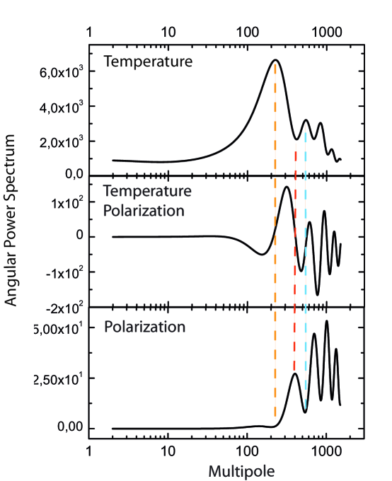
Figure 1: Theoretical predictions for the CMB temperature, polarization and cross temperature-polarization power spectra in the case of the standard model of structure formation. The peaks in the temperature and polarization spectra are alternate.

In Figure $1$ we plot the theoretical prediction for CMB temperature and polarization power spectra and the cross-correlation between temperature and polarization in the case of the so-called ’concordance’ model. The major conclusions we can draw from these predictions are:

• The power spectra show an unique structure: The temperature power spectrum is flat on large scale while shows oscillations on smaller scales. The polarization and cross temperature-polarization spectra are also showing oscillations on smaller scales, but the signal at large scale is expected to be negligible. This is a direct consequence of the fact that different physical mechanisms control the growth of perturbations on different scales.

• On smaller scales, again, different mechanisms are responsible for the oscillations. Gravity and density perturbations obey a cosine function, while velocity perturbations follow a sine function. On the scale of the thickness of the last scattering surface, temperature anisotropies are more coupled to density and gravity perturbations, while polarization is more coupled to velocity perturbations. The most striking observational prediction of this is the out-of-phase position of the peaks and dips in the temperature and polarization power spectra. The peaks and dips of the cross-correlation spectra fall in the middle.

• The shape of the power spectra depends on the value of the cosmological parameters assumed in the theoretical computation. A measure of these spectra can therefore produce indirect constraints on several parameters of the model. The parameters that can be well identified are the overall curvature, the energy density in baryons $\omega_{b}$, the energy density in dark matter $\omega_{m}$, the spectral tilt of primordial fluctuations $n_{S}$ and the value of the optical depth of the universe $\tau$. Presence of polarization at large angular scale, in particular, is evidence for a reionization of the intergalactic medium. Higher is the polarization at large scale, higher is the value of the optical of the universe at late redshifts. Since the overall picture must be consistent, the cosmological parameters determined indirectly from CMB observations must agree with the values inferred from independent observations (Big Bang Nucleosynthesis, Galaxy Surveys, Ly-$\alpha$ forest clouds, simulations, etc etc.).

10 The latest measurements.

The last years have been an exciting period for the field of the CMB research. With the TOCO$-97/98$ (torbet ,miller ) and BOOMERanG-$97$ (mauskopf ) experiments a firm detection of a first peak in the CMB angular power spectrum on about degree scales has been obtained. In the framework of adiabatic Cold Dark Matter (CDM) models, the position, amplitude and width of this peak provide strong supporting evidence for the inflationary predictions of a low curvature (flat) universe and a scale-invariant primordial spectrum (knox , melchiorri , tegb97 ).
The subsequent data from BOOMERanG LDB (netterfield ), DASI (halverson ), MAXIMA (lee ), VSAE (grainge ) and Archeops (benoit ) have provided further evidence for the presence of the first peak and refined the data at larger multipole hinting towards the presence of multiple peaks in the spectrum. Moreover, the very small scale observations made by the CBI (pearson ) and ACBAR (acbar ) experiments have confirmed the presence of a damping tail, while the new DASI results presented the first evidence for polarization (dasipol ).
The combined data clearly confirmed the model prediction of acoustic oscillations in the primeval plasma and shed new light on several cosmological and inflationary parameters ( see e.g. anze , odman , wang2 ).
The recent results from the WMAP satellite experiment (bennett ) have confirmed in a spectacular way all these previous results with a considerable reduction of the error bars. In particular, the amplitude and position of the first two peaks in the spectrum are now determined with a precision about $6$ times better than before (page ).
Furthermore, the WMAP team released the first high quality measurements of the temperature-polarization spectrum kogut . The presence of polarization at intermediate angular scale helps in discriminating inflationary models from causal scaling seed toy models. Moreover, the position of the first anti-peak and second peak in the spectrum are also in agreement with the prediction of inflation (dode ).
As main intriguing discrepancy, the WMAP data shows (in agreement with the previous COBE data) a lower temperature quadrupole than expected. The statistical significance of this discrepancy is still unclear (see e.g. costa , efstathiou2 , dore ).
The CMB anisotropies measured by WMAP are also in good agreement with the standard inflationary prediction of gaussianity (komatsu ).

11 CMB constraints on the standard model.

In principle, the standard scenario of structure formation based on adiabatic primordial fluctuations can depend on more than $11$ parameters.
However for a first analysis and under the assumption of a flat universe which is already well consistent with CMB data, it is possible to restrict ourselves to just $5$ parameters: the tilt of primordial spectrum of scalar perturbations $n_{S}$, the optical depth of the universe $\tau_{c}$, the physical energy densities in baryons and dark matter $\omega_{b}=\Omega_{b}h^{2}$ and $\omega_{dm}=\Omega_{dm}h^{2}$ and the Hubble parameter $h$.

	WMAP	WMAPext	WMAPext+LSS	Pre-WMAP+LSS
$\Omega_{b}h^{2}$	$0.024\pm 0.001$	$0.023\pm 0.001$	$0.023\pm 0.001$	$0.021\pm 0.003$
$\Omega_{m}h^{2}$	$0.14\pm 0.02$	$0.13\pm 0.01$	$0.134\pm 0.006$	$0.14\pm 0.02$
$h$	$0.72\pm 0.05$	$0.73\pm 0.05$	$0.73\pm 0.03$	$0.69\pm 0.07$
$n_{s}$	$0.99\pm 0.04$	$0.97\pm 0.03$	$0.97\pm 0.03$	$0.97\pm 0.04$
$\tau_{c}$	$0.166^{+0.076}_{-0.071}$	$0.143^{+0.071}_{-0.062}$	$0.148^{+0.073}_{-0.071}$	$0.07^{+0.07}_{-0.05}$

Table 1: Current constraints on the $5$ parameters of the standard model (flat universe). The WMAP results are taken from Spergel et al. 2003, the previous results are taken from Melchiorri and Odman 2003 (see also Slosar et al. 2003 and Wang et al. 2003).

In Table $1$ we report the constraints on these parameters obtained by the WMAP team (see spergel and verde ) in $3$ cases: WMAP only, WMAP+CBI+ACBAR and WMAP+CBI+ACBAR+LSS. Also, for comparison, we present the CMB+LSS results previous to WMAP in the forth column.
As we can see a value for the baryon density $\omega_{b}=0.020\pm 0.002$ as predicted by Standard Big Bang Nucleosynthesis (see e.g.cyburt ) is in very good agreement with the WMAP results. The WMAP data is in agreement with the previous results and its inclusion reduces the error bar on this parameter by a factor $3$.
The amount of cold dark matter is also well constrained by the CMB data. The presence of power around the third peak is crucial in this sense, since it cannot be easily accommodated in models based on just baryonic matter (see e.g. melksilk and references therein). As we can see, including the CMB data on those scales (not sampled by WMAP) halves the error bars. WMAP is again in agreement with the previous determination and its inclusion reduces the error bar on this parameter by of factor $3$-$4$.

These values implies the existence of a cosmological constant at high significance with $\Omega_{\Lambda}=0$, $\Omega_{M}=1$ excluded at $5$-$\sigma$ from the WMAP data alone and at $\sim 15$-$\sigma$ when combined with supernovae data. A cosmological constant is also suggested from the evidence of correlations of the WMAP data with large scale structure (scranton , nolta , boughn , afshordi ).

Under the assumption of flatness, is possible to constrain the value of the Hubble parameter $h$. The constraints on this parameter are in very well agreement with the HST constraint (freedman ).

An increase in the optical depth $\tau_{c}$ after recombination by reionization damps the amplitude of the CMB peaks. This small scale damping can be somewhat compensated by an increase in the spectral index $n_{S}$. This leads to a nearly perfect degeneracy between $n_{S}$ and $\tau_{c}$ and, in practice, no significant upper bound on these parameters can be placed from temperature data. However, large scale polarization data, as measured by WMAP, and LSS data can break this degeneracy. At the same time, inclusion of galaxy clustering data can determine $n_{S}$ and further break the degeneracy. As we can see, the current constraint on the spectral index is close to scale invariance ($n_{S}\sim 1$) as predicted by inflation. The best-fit value of the optical depth determined by WMAP is slightly higher but consistent in between $1-\sigma$ with supercomputer simulations of reionization processes ($\tau_{c}\sim 0.10$, see e.g. ciardi ).

12 Constraints on possible extensions of the standard model.

The standard model provides a reasonable fit to the data. However it is possible to consider several modifications characterized by the inclusion of new parameters. The data considered here doesn’t show any definite evidence for those modifications, providing more a set of useful constraints. The present constraints are as follows:

• Running of the Spectral Index

  The possibility of a scale dependence of the scalar spectral index, $n_{S}(k)$, has been considered in various works (see e.g. kosowsky , AMcopeland , doste ). Even though this dependence is considered to have small effects on CMB scales in most of the slow-roll inflationary models, it is worthwhile to see if any useful constraint can be obtained. The present CMB data is at the moment compatible with no scale dependence (kkmr ,bridle ), however, joint analyses with other datasets (like Lyman-$\alpha$) shows a $\sim 2-\sigma$ evidence for a negative running (peiris ). At the moment, the biggest case against running comes from reionization models, which are unable to reach the large optical depth observed in this case by WMAP ($\tau\sim 0.17$, see spergel ) with the suppressed power on small scales (see e.g. cen ).

• Gravitational Waves.

  The metric perturbations created during inflation belong to two types: scalar perturbations, which couple to the stress-energy of matter in the universe and form the “seeds” for structure formation and tensor perturbations, also known as gravitational wave perturbations. A sizable background of gravity waves is expected in most of the inflationary scenarios and a detection of the GW background can provide information on the second derivative of the inflaton potential and shed light on the physics at $\sim 10^{16}Gev$.

  The amplitude of the GW background is weakly constrained by the current CMB data. However, when information from BBN, local cluster abundance and galaxy clustering are included, an upper limit of about $r=C_{2}^{T}/C_{2}^{S}<0.5$ (no running) is obtained (see e.g. spergel , kkmr , barger , leach ).

• Isocurvature Perturbations

  Another key assumption of the standard model is that the primordial fluctuations were adiabatic. Adiabaticity is not a necessary consequence of inflation though and many inflationary models have been constructed where isocurvature perturbations would have generically been concomitantly produced (see e.g. langlois , gordon , bartolo ). Pure isocurvature perturbations are highly excluded by present CMB data. Due to degeneracies with other cosmological parameters, the amount of isocurvature modes is still weakly constrained by the present data (see e.g. peiris , jussi , AMcrotty ).

• Modified recombination.

  The standard recombination process can be modified in several ways. Extra sources of ionizing and resonance radiation at recombination or having a time-varying fine-structure constant, for example, can delay the recombination process and leave an imprint on the CMB anisotropies. The present data is in agreement with the standard recombinations scheme. However, non-standard recombination scenarios are still consistent with the current data and may affect the current WMAP constraints on inflationary parameters like the spectral index, $n_{s}$, and its running (see e.g. avelino , martins , bms ).

• Neutrino Physics

  The effective number of neutrinos and their effective mass can be both constrained by combining cosmological data. The combination of present cosmological data under the assumption of several priors provide a constraint on the effective neutrino mass of $m_{ee}<0.23eV$ (spergel ). The data constraints the effective number of neutrino species to about $N_{eff}<7$ (see e.g. pierpaoli , julien ,hannestad ).

• Dark Energy and its equation of state

  The discovery that the universe’s evolution may be dominated by an effective cosmological constant is one of the most remarkable cosmological findings of recent years. Observationally distinguishing a time variation in the equation of state or finding it different from $-1$ is a powerful test for the cosmological constant. The present constraints on $w$ obtained combining the CMB data with several other cosmological datasets are consistent with $w=-1$, with models with $w<-1$ slightly preferred (see e.g. mmot , wlewis ). Other dark energy parameters, like its sound speed, are weakly constrained (bo , caldwell ).

13 Conclusions

The recent CMB data represent a beautiful success for the standard cosmological model. The acoustic oscillations in the CMB temperature power spectrum, a major prediction of the model, have now been detected with high statistical significance. The amplitude and shape of the cross correlation temperature-polarization power spectrum is also in agreement with the expectations.

Furthermore, when constraints on cosmological parameters are derived under the assumption of adiabatic primordial perturbations their values are in agreement with the predictions of the theory and/or with independent observations.

The largest discrepancy between the standard predictions and the data seems to come from the low value of the CMB quadrupole. New physics has been proposed to explain this discrepancy (see e.g. contaldi , freese , luminet ), but the statistical significance is of difficult interpretation.

As we saw in the previous section modifications as isocurvature modes or topological defects, are still compatible with current CMB observations, but are not necessary and can be reasonably constrained when complementary datasets are included.

14 Acknowledgements

I wish to thank the organizers of the conference: Norma Mankoc Borstnik and Holger Bech Nielsen. Many thanks also to Rachel Bean, Will Kinney, Rocky Kolb, Carlos Martins, Laura Mersini, Roya Mohayaee, Carolina Oedman, Antonio Riotto, Graca Rocha, Joe Silk, and Mark Trodden for comments, discussions and help.

*AdS/CFT Correspondence and Unification at About 4 TeV Paul H. Frampton

15 Introduction

I will give a brief summary of an approach to string phenomenology which is inspired by AdS/CFT correspondence and which has been pursued for the last five years. Finite-N non-SUSY theories as discussed here are not obtainable from AdS/CFT although a speculation, currently under study, is that key UV properties of infinite-N theories which may be so obtained can survive, at least in some(one?) cases for the finite-N case. Future work will study the (non-)occurrence of quadratic divergences in the resultant finite-N gauge theories.

Independent of the outcome of that study, interesting possibilities emerge for extending the standard model without low-energy supersymmetry. These possibilities would become far more compelling if the quadratic divergences associated with fundamental scalars can indeed be eliminated.

16 Quiver Gauge Theory

The relationship of the Type IIB superstring to conformal gauge theory in $d=4$ gives rise to an interesting class of gauge theories. Choosing the simplest compactificationMaldacena on $AdS_{5}\times S_{5}$ gives rise to an ${\cal N}=4$ SU(N) gauge theory which is known to be conformal due to the extended global supersymmetry and non-renormalization theorems. All of the RGE $\beta-$functions for this ${\cal N}=4$ case are vanishing in perturbation theory. It is possible to break the ${\cal N}=4$ to ${\cal N}=2,1,0$ by replacing $S_{5}$ by an orbifold $S_{5}/\Gamma$ where $\Gamma$ is a discrete group with $\Gamma\subset SU(2),\subset SU(3),\not\subset SU(3)$ respectively.

In building a conformal gauge theory model Frampton ; FS ; FV , the steps are: (1) Choose the discrete group $\Gamma$; (2) Embed $\Gamma\subset SU(4)$; (3) Choose the $N$ of $SU(N)$; and (4) Embed the Standard Model $SU(3)\times SU(2)\times U(1)$ in the resultant gauge group $\bigotimes SU(N)^{p}$ (quiver node identification). Here we shall look only at abelian $\Gamma=Z_{p}$ and define $\alpha=exp(2\pi i/p)$. It is expected from the string-field duality that the resultant field theory is conformal in the $N\longrightarrow\infty$ limit, and will have a fixed manifold, or at least a fixed point, for $N$ finite.

Before focusing on ${\cal N}=0$ non-supersymmetric cases, let us first examine an ${\cal N}=1$ model first put forward in the work of Kachru and SilversteinKS . The choice is $\Gamma=Z_{3}$ and the 4 of $SU(4)$ is 4 = $(1,\alpha,\alpha,\alpha^{2})$. Choosing N=3 this leads to the three chiral families under $SU(3)^{3}$ trinificationDGG

$$(3,\bar{3},1)+(1,3,\bar{3})+(\bar{3},1,3)$$ (41)

17 Gauge Couplings.

An alternative to conformality, grand unification with supersymmetry, leads to an impressively accurate gauge coupling unificationADFFL . In particular it predicts an electroweak mixing angle at the Z-pole, ${\tt sin}^{2}\theta=0.231$. This result may, however, be fortuitous, but rather than abandon gauge coupling unification, we can rederive ${\tt sin}^{2}\theta=0.231$ in a different way by embedding the electroweak $SU(2)\times U(1)$ in $SU(N)\times SU(N)\times SU(N)$ to find ${\tt sin}^{2}\theta=3/13\simeq 0.231$FV ; F2 . This will be a common feature of the models in this paper.

18 4 TeV Grand Unification

Conformal invariance in two dimensions has had great success in comparison to several condensed matter systems. It is an interesting question whether conformal symmetry can have comparable success in a four-dimensional description of high-energy physics.

Even before the standard model (SM) $SU(2)\times U(1)$ electroweak theory was firmly established by experimental data, proposals were made PS ; GG of models which would subsume it into a grand unified theory (GUT) including also the dynamicsGQW of QCD. Although the prediction of SU(5) in its minimal form for the proton lifetime has long ago been excluded, ad hoc variants thereof FG remain viable. Low-energy supersymmetry improves the accuracy of unification of the three 321 couplingsADF ; ADFFL and such theories encompass a “desert” between the weak scale $\sim 250$ GeV and the much-higher GUT scale $\sim 2\times 10^{16}$ GeV, although minimal supersymmetric $SU(5)$ is by now ruled outMurayama .

Recent developments in string theory are suggestive of a different strategy for unification of electroweak theory with QCD. Both the desert and low-energy supersymmetry are abandoned. Instead, the standard $SU(3)_{C}\times SU(2)_{L}\times U(1)_{Y}$ gauge group is embedded in a semi-simple gauge group such as $SU(3)^{N}$ as suggested by gauge theories arising from compactification of the IIB superstring on an orbifold $AdS_{5}\times S^{5}/\Gamma$ where $\Gamma$ is the abelian finite group $Z_{N}$Frampton . In such nonsupersymmetric quiver gauge theories the unification of couplings happens not by logarithmic evolutionGQW over an enormous desert covering, say, a dozen orders of magnitude in energy scale. Instead the unification occurs abruptly at $\mu=M$ through the diagonal embeddings of 321 in $SU(3)^{N}$F2 . The key prediction of such unification shifts from proton decay to additional particle content, in the present model at $\simeq 4$ TeV.

Let me consider first the electroweak group which in the standard model is still un-unified as $SU(2)\times U(1)$. In the 331-modelPP ; PF where this is extended to $SU(3)\times U(1)$ there appears a Landau pole at $M\simeq 4$ TeV because that is the scale at which ${\rm sin}^{2}\theta(\mu)$ slides to the value ${\rm sin}^{2}(M)=1/4$. It is also the scale at which the custodial gauged $SU(3)$ is broken in the framework of DK .

There remains the question of embedding such unification in an $SU(3)^{N}$ of the type described in Frampton ; F2 . Since the required embedding of $SU(2)_{L}\times U(1)_{Y}$ into an $SU(3)$ necessitates $3\alpha_{Y}=\alpha_{H}$ the ratios of couplings at $\simeq 4$ TeV is: $\alpha_{3C}:\alpha_{3W}:\alpha_{3H}::5:2:2$ and it is natural to examine $N=12$ with diagonal embeddings of Color (C), Weak (W) and Hypercharge (H) in $SU(3)^{2},SU(3)^{5},SU(3)^{5}$ respectively.

To accomplish this I specify the embedding of $\Gamma=Z_{12}$ in the global $SU(4)$ R-parity of the ${\cal N}=4$ supersymmetry of the underlying theory. Defining $\alpha={\rm exp}(2\pi i/12)$ this specification can be made by ${\bf 4}\equiv(\alpha^{A_{1}},\alpha^{A_{2}},\alpha^{A_{3}},\alpha^{A_{4}})$ with $\Sigma A_{\mu}=0({\rm mod}12)$ and all $A_{\mu}\not=0$ so that all four supersymmetries are broken from ${\cal N}=4$ to ${\cal N}=0$.

Having specified $A_{\mu}$ I calculate the content of complex scalars by investigating in $SU(4)$ the ${\bf 6}\equiv(\alpha^{a_{1}},\alpha^{a_{2}},\alpha^{a_{3}},\alpha^{-a_{3}},\alpha^{-a_{2}},\alpha^{-a_{1}})$ with $a_{1}=A_{1}+A_{2},a_{2}=A_{2}+A_{3},a_{3}=A_{3}+A_{1}$ where all quantities are defined (mod 12).

Finally I identify the nodes (as C, W or H) on the dodecahedral quiver such that the complex scalars

$$\Sigma_{i=1}^{i=3}\Sigma_{\alpha=1}^{\alpha=12}\left(N_{\alpha},\bar{N}_{\alpha\pm a_{i}}\right)$$ (42)

are adequate to allow the required symmetry breaking to the $SU(3)^{3}$ diagonal subgroup, and the chiral fermions

$$\Sigma_{\mu=1}^{\mu=4}\Sigma_{\alpha=1}^{\alpha=12}\left(N_{\alpha},\bar{N}_{\alpha+A_{\mu}}\right)$$ (43)

can accommodate the three generations of quarks and leptons.

It is not trivial to accomplish all of these requirements so let me demonstrate by an explicit example.

For the embedding I take $A_{\mu}=(1,2,3,6)$ and for the quiver nodes take the ordering:

$$-C-W-H-C-W^{4}-H^{4}-$$ (44)

with the two ends of (44) identified.

The scalars follow from $a_{i}=(3,4,5)$ and the scalars in Eq.(42)

$$\Sigma_{i=1}^{i=3}\Sigma_{\alpha=1}^{\alpha=12}\left(3_{\alpha},\bar{3}_{\alpha\pm a_{i}}\right)$$ (45)

are sufficient to break to all diagonal subgroups as

$$SU(3)_{C}\times SU(3)_{W}\times SU(3)_{H}$$ (46)

The fermions follow from $A_{\mu}$ in Eq.(43) as

$$\Sigma_{\mu=1}^{\mu=4}\Sigma_{\alpha=1}^{\alpha=12}\left(3_{\alpha},\bar{3}_{\alpha+A_{\mu}}\right)$$ (47)

and the particular dodecahedral quiver in (44) gives rise to exactly three chiral generations which transform under (46) as

$$3[(3,\bar{3},1)+(\bar{3},1,3)+(1,3,\bar{3})]$$ (48)

I note that anomaly freedom of the underlying superstring dictates that only the combination of states in Eq.(48) can survive. Thus, it is sufficient to examine one of the terms, say $(3,\bar{3},1)$. By drawing the quiver diagram indicated by Eq.(44) with the twelve nodes on a “clock-face” and using $A_{\mu}=(1,2,3,6)$ I find five $(3,\bar{3},1)$’s and two $(\bar{3},3,1)$’s implying three chiral families as stated in Eq.(48).

After further symmetry breaking at scale $M$ to $SU(3)_{C}\times SU(2)_{L}\times U(1)_{Y}$ the surviving chiral fermions are the quarks and leptons of the SM. The appearance of three families depends on both the identification of modes in (44) and on the embedding of $\Gamma\subset SU(4)$. The embedding must simultaneously give adequate scalars whose VEVs can break the symmetry spontaneously to (46). All of this is achieved successfully by the choices made. The three gauge couplings evolve for $M_{Z}\leq\mu\leq M$. For $\mu\geq M$ the (equal) gauge couplings of $SU(3)^{12}$ do not run if, as conjectured in Frampton ; F2 there is a conformal fixed point at $\mu=M$.

The basis of the conjecture in Frampton ; F2 is the proposed duality of MaldacenaMaldacena which shows that in the $N\rightarrow\infty$ limit ${\cal N}=4$ supersymmetric $SU(N)$gauge theory, as well as orbifolded versions with ${\cal N}=2,1$ and $0$bershadsky1 ; bershadsky2 become conformally invariant. It was known long ago that the ${\cal N}=4$ theory is conformally invariant for all finite ${\cal N}\geq 2$. This led to the conjecture in Frampton that the ${\cal N}=0$ theories might be conformally invariant, at least in some case(s), for finite $N$. It should be emphasized that this conjecture cannot be checked purely within a perturbative frameworkFMink . I assume that the local $U(1)$’s which arise in this scenario and which would lead to $U(N)$ gauge groups are non-dynamical, as suggested by WittenWitten , leaving $SU(N)$’s.

As for experimental tests of such a TeV GUT, the situation at energies below 4 TeV is predicted to be the standard model with a Higgs boson still to be discovered at a mass predicted by radiative corrections PDG to be below 267 GeV at 99% confidence level.

There are many particles predicted at $\simeq 4$ TeV beyond those of the minimal standard model. They include as spin-0 scalars the states of Eq.(45). and as spin-1/2 fermions the states of Eq.(47), Also predicted are gauge bosons to fill out the gauge groups of (46), and in the same energy region the gauge bosons to fill out all of $SU(3)^{12}$. All these extra particles are necessitated by the conformality constraints of Frampton ; F2 to lie close to the conformal fixed point.

One important issue is whether this proliferation of states at $\sim 4$ TeV is compatible with precision electroweak data in hand. This has been studied in the related model of DK in a recent articleCsaki . Those results are not easily translated to the present model but it is possible that such an analysis including limits on flavor-changing neutral currents could rule out the entire framework.

19 Predictivity

The calculations have been done in the one-loop approximation to the renormalization group equations and threshold effects have been ignored. These corrections are not expected to be large since the couplings are weak in the entrire energy range considered. There are possible further corrections such a non-perturbative effects, and the effects of large extra dimensions, if any.

In one sense the robustness of this TeV-scale unification is almost self-evident, in that it follows from the weakness of the coupling constants in the evolution from $M_{Z}$ to $M_{U}$. That is, in order to define the theory at $M_{U}$, one must combine the effects of threshold corrections ( due to O($\alpha(M_{U})$) mass splittings ) and potential corrections from redefinitions of the coupling constants and the unification scale. We can then impose the coupling constant relations at $M_{U}$ as renormalization conditions and this is valid to the extent that higher order corrections do not destabilize the vacuum state.

We shall approach the comparison with data in two different but almost equivalent ways. The first is ”bottom-up” where we use as input that the values of $\alpha_{3}(\mu)/\alpha_{2}(\mu)$ and $\sin^{2}\theta(\mu)$ are expected to be $5/2$ and $1/4$ respectively at $\mu=M_{U}$.

Using the experimental ranges allowed for $\sin^{2}\theta(M_{Z})=0.23113\pm 0.00015$, $\alpha_{3}(M_{Z})=0.1172\pm 0.0020$ and $\alpha_{em}^{-1}(M_{Z})=127.934\pm 0.027$ PDG we have calculated FRT the values of $\sin^{2}\theta(M_{U})$ and $\alpha_{3}(M_{U})/\alpha_{2}(M_{U})$ for a range of $M_{U}$ between 1.5 TeV and 8 TeV. Allowing a maximum discrepancy of $\pm 1\%$ in $\sin^{2}\theta(M_{U})$ and $\pm 4\%$ in $\alpha_{3}(M_{U})/\alpha_{2}(M_{U})$ as reasonable estimates of corrections, we deduce that the unification scale $M_{U}$ can lie anywhere between 2.5 TeV and 5 TeV. Thus the theory is robust in the sense that there is no singular limit involved in choosing a particular value of $M_{U}$.

Another test of predictivity of the same model is to fix the unification values at $M_{U}$ of $\sin^{2}\theta(M_{U})=1/4$ and $\alpha_{3}(M_{U})/\alpha_{2}(M_{U})=5/2$. We then compute the resultant predictions at the scale $\mu=M_{Z}$.

The results are shown for $\sin^{2}\theta(M_{Z})$ in FRT with the allowed rangePDG $\alpha_{3}(M_{Z})=0.1172\pm 0.0020$. The precise data on $\sin^{2}(M_{Z})$ are indicated in FRT and the conclusion is that the model makes correct predictions for $\sin^{2}\theta(M_{Z})$. Similarly, in FRT , there is a plot of the prediction for $\alpha_{3}(M_{Z})$ versus $M_{U}$ with $\sin^{2}\theta(M_{Z})$ held with the allowed empirical range. The two quantities plotted in FRT are consistent for similar ranges of $M_{U}$. Both $\sin^{2}\theta(M_{Z})$ and $\alpha_{3}(M_{Z})$ are within the empirical limits if $M_{U}=3.8\pm 0.4$ TeV.

The model has many additional gauge bosons at the unification scale, including neutral $Z^{{}^{\prime}}$’s, which could mediate flavor-changing processes on which there are strong empirical upper limits.

A detailed analysis wll require specific identification of the light families and quark flavors with the chiral fermions appearing in the quiver diagram for the model. We can make only the general observation that the lower bound on a $Z^{{}^{\prime}}$ which couples like the standard $Z$ boson is quoted as $M(Z^{{}^{\prime}})<1.5$ TeV PDG which is safely below the $M_{U}$ values considered here and which we identify with the mass of the new gauge bosons.

This is encouraging to believe that flavor-changing processes are under control in the model but this issue will require more careful analysis when a specific identification of the quark states is attempted.

Since there are many new states predicted at the unification scale $\sim 4$ TeV, there is a danger of being ruled out by precision low energy data. This issue is conveniently studied in terms of the parameters $S$ and $T$ introduced in Peskin and designed to measure departure from the predictions of the standard model.

Concerning $T$, if the new $SU(2)$ doublets are mass-degenerate and hence do not violate a custodial $SU(2)$ symmetry they contribute nothing to $T$. This therefore provides a constraint on the spectrum of new states.

20 Discussion

The plots we have presented clarify the accuracy of the predictions of this TeV unification scheme for the precision values accurately measured at the Z-pole. The predictivity is as accurate for $\sin^{2}\theta$ as it is for supersymmetric GUT modelsADFFL ; ADF ; DRW ; DG . There is, in addition, an accurate prediction for $\alpha_{3}$ which is used merely as input in SusyGUT models.

At the same time, the accurate predictions are seen to be robust under varying the unification scale around $\sim 4TeV$ from about 2.5 TeV to 5 TeV.

One interesting question is concerning the accommodation of neutrino masses in view of the popularity of the mechanisms which require a higher mass scale than occurs in the present type of model. For example, one would like to know whether any of the recent studies in FGMY can be useful within this framework.

In conclusion, since this model ameliorates the GUT hierarchy problem and naturally accommodates three families, it provides a viable alternative to the widely-studied GUT models which unify by logarithmic evolution of couplings up to much higher GUT scales.

*New Solutions in String Field Theory Loriano Bonora

21 Introduction

Recently, as a consequence of the increasing interest in tachyon condensation, String Field Theory (SFT) has received renewed attention. There is no doubt that the most complete description of tachyon condensation and related phenomena has been given so far in the framework of Witten’s Open String Field Theory, W1 . This is not surprising, since the study of tachyon condensation involves off–shell calculations, and SFT is the natural framework where off–shell analysis can be carried out.

All these developments can be described in terms of Sen’s conjectures, Sen . Sen’s conjectures can be summarized as follows. Bosonic open string theory in D=26 dimensions is quantized on an unstable vacuum, an instability which manifests itself through the existence of the open string tachyon. The effective tachyonic potential has, beside the local maximum where the theory is quantized, a local minimum. Sen’s conjectures concern the nature of the theory around this local minimum. First of all, the energy density difference between the maximum and the minimum should exactly compensate for the D25–brane tension characterizing the unstable vacuum: this is a condition for the stability of the theory at the minimum. Therefore the theory around the minimum should not contain any quantum fluctuation pertaining to the original (unstable) theory. The minimum should therefore correspond to an entirely new theory, the bosonic closed string theory. If so, in the new theory one should be able to explicitly find in particular all the classical solutions characteristic of closed string theory, specifically the D25–brane as well as all the lower dimensional D–branes.

The evidence that has been collected so far for the above conjectures does not have a uniform degree of accuracy and reliability, but it is enough to conclude that they provide a correct description of tachyon condensation in SFT. Especially elegant is the proof of the existence of solitonic solutions in Vacuum String Field Theory (VSFT), the SFT version which is believed to represent the theory near the minimum.

A time-dependent solution which describes the evolution from the maximum of the tachyon potential to such a minimum (a rolling tachyon), if it exists, would describe the decay of the D25–brane into closed string states. It has been argued in many ways that such a solution exists; in particular this has led to the formulation of a new kind of duality between open and closed strings. But all this has been possible so far only outside a SFT framework. It would make an important progress if we could describe the rolling tachyon solution and the open–closed string duality in the framework of SFT.

In this regard VSFT could play an important role. VSFT is a simplified version of SFT, in which the BRST operator ${\cal Q}$ takes a very simple form in terms of ghost oscillators alone. It is clearly simpler to work in such a framework than in the original SFT. In fact many classical solutions have been shown to exist, which are candidates for representing D–branes (the sliver,the butterfly,etc), and other classical solutions have been found (lump solutions) which may represent lower dimensional D–branes. In some cases the spectrum around such solutions have been analyzed and some aspects of the D–brane spectrum have been reproduced. However the responses of VSFT are still far from being satisfactory. There are a series of nontrivial problems left behind. Let us consider for definitness the sliver solution. To start with it has vanishing action for the matter part and infinite action for the ghost part, but it is impossible to get a finite number out of them. Second, it is not at all clear whether the solutions of the linear equations of motion around the sliver can accommodate all the open string modes (as one would expect if the sliver has to represent a D25–brane). Third, the other Virasoro constraints on such modes are nowhere to be seen.

We believe that these drawbacks are due to the fact that the sliver is not the most suitable solution to represent a D25–brane. On the other hand the sliver has many interesting properties: it is simple and algebraically appealing (it is a squeezed state), its structure matrix $CS$ commutes with the twisted matrices of the three strings vertex coefficients and the calculations involving the sliver are relatively simple. Therefore in order to define a new solution we choose to stay as close as possible to the sliver. In practice we start from the sliver and ‘perturb it’ by adding to $CS$ a suitable rank one projector. We can show not only that this is a solution of the VSFT equations of motion, but that we can define infinite many independent such solutions. We call such solutions dressed slivers. They are characterized by finite norm and action.

In this contribution I will limit myself to showing how one arrives at the definition of the dressed sliver solution. The explicit calculations as well as other properties of this solution are reported in two research papers, BMP1 ; BMP2 .

22 A review of SFT and VSFT

Let us start with a short review of SFT à la Witten. The open string field theory action proposed by E.Witten, W1 , years ago is

$${\cal S}(\Psi)=-\frac{1}{g_{0}^{2}}\int\left(\frac{1}{2}\Psi*Q\Psi+\frac{1}{3}\Psi*\Psi*\Psi\right)$$ (49)

In this expression $\Psi$ is the string field, which can be understood either as a classical functional of the open string configurations or as a vector in the Fock space of states of the open string. We will consider in the following the second point of view. In the field theory limit it makes sense to represent it as a superposition of Fock space states with ghost number 1, with coefficient represented by local fields,

$$|{\Psi}\rangle=(\phi(x)+A_{\mu}(x)a_{1}^{\mu\dagger}+\ldots)c_{1}|{0}\rangle$$ (50)

The BRST charge $Q$ has the same form as in the first quantized string theory. The star product of two string fields $\Psi_{1},\Psi_{2}$ represents the process of identifying the right half of the first string with the left half of the second string and integrating over the overlapping degrees of freedom, to produce a third string which corresponds to $\Psi_{1}*\Psi_{2}$. This can be done in various ways, either using the classical string functionals (as in the original formulation), or using the three string vertex (see below), or the conformal field theory language leclair1 . Finally the integration in (49) corresponds to bending the left half of the string over the right half and integrating over the corresponding degrees of freedom in such a way as to produce a number. The following rules are obeyed

$$Q^{2}=0$$

$$\int Q\Psi=0$$

$$(\Psi_{1}*\Psi_{2})*\Psi_{3}=\Psi_{1}*(\Psi_{2}*\Psi_{3})$$

$$Q(\Psi_{1}*\Psi_{2})=(Q\Psi_{1})*\Psi_{2}+(-1)^{|\Psi_{1}|}\Psi_{1}*(Q\Psi_{2})$$ (51)

where $|\Psi|$ is the Grassmannality of the string field $\Psi$, which, for bosonic strings, coincides with the ghost number. The action (49) is invariant under the BRST transformation

$$\delta\Psi=Q\Lambda+\Psi*\Lambda-\Lambda*\Psi$$ (52)

Finally, the ghost numbers of the various objects $Q,\Psi,\Lambda,*,\int$ are $1,1,0,0,-3$, respectively.

22.1 Vacuum string field theory

The action (49) represents open string theory about the trivial unstable vacuum $|\Psi_{0}\rangle=c_{1}|0\rangle$. Vacuum string field theory (VSFT) is instead a version of Witten’s open SFT which is conjectured to correspond to the minimum of the tachyon potential. As explained in the introduction, at the minimum of the tachyon potential a dramatic change occurs in the theory, which, corresponding to the new vacuum, is expected to represent closed string theory rather that the open string theory we started with. In particular, this theory should host tachyonic lumps representing unstable D–branes of any dimension less than 25, beside the original D25–brane. Unfortunately we have been so far unable to find an exact classical solution, say $|\Phi_{0}\rangle$, representing the new vacuum. One can nevertheless guess the form taken by the theory at the new minimum, see RSZ1 . The VSFT action has the same form as (49), where the new string field is still denoted by $\Psi$, the $*$ product is the same as in the previous theory, while the BRST operator $Q$ is replaced by a new one, usually denoted ${\cal Q}$, which is characterized by universality and vanishing cohomology. Relying on such general arguments, one can even deduce a precise form of $\cal Q$, HKw ; GRSZ1 ,

$${\cal{Q}}=c_{0}+\sum_{n>0}\,(-1)^{n}\,(c_{2n}+c_{-2n})$$ (53)

Now, the equation of motion of VSFT is

$${\cal Q}\Psi=-\Psi*\Psi$$ (54)

and nonperturbative solutions are looked for in the factorized form

$$\Psi=\Psi_{m}\otimes\Psi_{g}$$ (55)

where $\Psi_{g}$ and $\Psi_{m}$ depend purely on ghost and matter degrees of freedom, respectively. Then eq.(54) splits into

$${\cal Q}\Psi_{g} = -\Psi_{g}*_{g}\Psi_{g}$$ (56)

$$\Psi_{m} = \Psi_{m}*_{m}\Psi_{m}$$ (57)

The action for this type of solutions becomes

$${\cal S}(\Psi)=-\frac{1}{6g_{0}^{2}}\langle\Psi_{g}|{\cal Q}|\Psi_{g}\rangle\langle\Psi_{m}|\Psi_{m}\rangle$$ (58)

In the following, for simplicity, we will limit myself to the matter part. $\langle\Psi_{m}|\Psi_{m}\rangle$ is the ordinary inner product, $\langle\Psi_{m}|$ being the $bpz$ conjugate of $|\Psi_{m}\rangle$ (see below).

Since here we are interested in the D25–brane, which is translational invariant, the $*_{m}$ product is simply defined as follows

$$\langle V_{3}|\Psi_{1}\rangle_{1}\Psi_{2}\rangle_{2}=_{3}\langle\Psi_{1}*_{m}\Psi_{2}|$$ (59)

where the reduced three strings vertex $V_{3}$ is defined by

$$|V_{3}\rangle={\rm exp}(-E)\,|0\rangle_{123},\quad\quad E=\frac{1}{2}\sum_{a,b=1}^{3}\sum_{m,n\geq 1}\eta_{\mu\nu}a_{m}^{(a)\mu\dagger}V_{mn}^{ab}a_{n}^{(b)\nu\dagger}$$ (60)

Summation over the Lorentz indices $\mu,\nu=0,\ldots,25$ is understood and $\eta$ denotes the flat Lorentz metric. The operators $a_{m}^{(a)\mu},a_{m}^{(a)\mu\dagger}$ denote the non–zero modes matter oscillators of the $a$–th string, which satisfy

$$[a_{m}^{(a)\mu},a_{n}^{(b)\nu\dagger}]=\eta^{\mu\nu}\delta_{mn}\delta^{ab},\quad\quad m,n\geq 1$$ (61)

Moreover $|0\rangle_{123}=|0\rangle_{1}\otimes|0\rangle_{2}\otimes|0\rangle_{3}$ is the tensor product of the Fock vacuum states relative to the three strings. The symbols $V_{nm}^{ab},V_{0m}^{ab},V_{00}^{ab}$ will denote the coefficients computed in GJ1 . We will use them in the notation of Appendix A and B of RSZ2 .

To complete the definition of the $*_{m}$ product we must specify the $bpz$ conjugation properties of the oscillators

$$bpz(a_{n}^{(a)\mu})=(-1)^{n+1}a_{-n}^{(a)\mu}$$

22.2 The sliver solution

Let us now return to eq.(57). Its solutions are projectors of the $*_{m}$ algebra. We recall the simplest one, the sliver. It is defined by

$$|\Xi\rangle=\cal{N}e^{-\frac{1}{2}a^{\dagger}Sa^{\dagger}},\quad\quad a^{\dagger}Sa^{\dagger}=\sum_{n,m=1}^{\infty}a_{n}^{\mu\dagger}S_{nm}a_{m}^{\nu\dagger}\eta_{\mu\nu}$$ (62)

This state satisfies eq.(57) provided the matrix $S$ satisfies the equation

$$S=V^{11}+(V^{12},V^{21})({\bf I}-\Sigma{\cal V})^{-1}\Sigma\left(\begin{matrix}V^{21}\cr V^{12}\end{matrix}\right)$$ (63)

where

$$\Sigma=\left(\begin{matrix}S&0\cr 0&S\end{matrix}\right),\quad\quad\quad{\cal V}=\left(\begin{matrix}V^{11}&V^{12}\cr V^{21}&V^{22}\end{matrix}\right),$$ (64)

The proof of this fact is well–known, KP . First one expresses eq.(64) in terms of the twisted matrices $X=CV^{11},X_{+}=CV^{12}$ and $X_{-}=V^{21}$, together with $T=CS=SC$, where $C_{nm}=(-1)^{n}\delta_{nm}$. The matrices $X,X_{+},X_{-}$ are mutually commuting. Then, requiring that $T$ commute with them as well, one can show that eq.(64) reduces to the algebraic equation

$$XT^{2}-(1+X)T+X=0$$ (65)

The interesting solution is

$$T=\frac{1}{2X}(1+X-\sqrt{(1+3X)(1-X)})$$ (66)

The normalization constant $\cal{N}$ is calculated to be

$$\cal{N}=(\det(1-\Sigma\cal{V}))^{13}$$ (67)

The contribution of the sliver to the matter part of the action (see (58) is given by

$$\langle\Xi|\Xi\rangle=\frac{\cal{N}^{2}}{(\det(1-S^{2}))^{13}}$$ (68)

Both eq.(67) and (68) are ill–defined and need to be regularized, after which they both result to be vanishing (see below).

23 The dressed sliver solution

Now we want to deform the sliver by adding some special matrix to $S$. To this end first we introduce the infinite vector $\xi=\{\xi_{n}\}$ which are chosen to satisfy the condition

$$\rho_{1}\xi=0,\quad\quad\rho_{2}\xi=\xi,$$ (69)

The operators $\rho_{1},\rho_{2}$ are Fock space projectors into (left or right) half string states. Next we require $\xi$ to be real and set

$$\xi^{T}\frac{1}{1-T^{2}}\xi=1,\quad\quad\xi^{T}\frac{T}{1-T^{2}}\xi=\kappa$$ (70)

$\kappa$ turns out to be a negative real number. We remark that the conditions (70) are not very stringent. The only thing one has to worry is that the LHS’s are finite (this is the only true condition). Once this is true the rest follows from suitably rescaling $\xi$, so that the first equation is satisfied, and from the reality of $\xi$.

Our candidate for the dressed sliver solution is given by an ansatz similar to (62)

$$|\hat{\Xi}\rangle=\hat{\cal N}e^{-\frac{1}{2}a^{\dagger}\hat{S}a^{\dagger}},$$ (71)

with $S$ replaced by

$$\hat{S}=S+R,\quad\quad R_{nm}=\frac{1}{\kappa+1}\left(\xi_{n}(-1)^{m}\xi_{m}+\xi_{m}(-1)^{n}\xi_{n}\right)$$ (72)

As a consequence $\hat{T}$ is replaced by

$$\hat{T}_{\epsilon}=T+P,\quad\quad P_{nm}=\frac{1}{\kappa+1}\left(\xi_{n}(-1)^{m+n}\xi_{m}+\xi_{m}\xi_{n}\right)$$ (73)

The dressed sliver satisfies hermiticity.

We claim that $|\hat{\Xi}\rangle$ is a projector. The dressed sliver matrix $\hat{T}$ does not commute with $X,X_{-},X_{+}$ (as T does), but we can nevertheless make use of the property $C\hat{T}=\hat{T}C$, because $CP=PC$. Using this it is in fact possible to show, BMP1 , that

$$V^{11}+(V^{12},V^{21})({1}-\hat{\Sigma}{\cal V})^{-1}\hat{\Sigma}\left(\begin{matrix}V^{21}\cr V^{12}\end{matrix}\right)=\hat{S}$$ (74)

where

$$\hat{\Sigma}=\left(\begin{matrix}\hat{S}&0\cr 0&\hat{S}\end{matrix}\right)$$ (75)

The defintion (71) is not yet satisfactory. The reason is that its normalization and the corresponding action are still ill-defined. We have to supplement the above definition with some specification. To this end we introduce in (71) a deformation parameter ${\epsilon}$, which multiplies $R$, i.e. $\hat{S}\to\hat{S}_{\epsilon}=S+{\epsilon}R$. In this way we obtain a state $\hat{\Xi}_{\epsilon}$ which interpolates between the sliver $\epsilon=0$ and the dressed sliver $\epsilon=1$. Now, interpreting it as a sequence of states in the vicinity of $\epsilon=1$, we can give a precise definition of the dressed sliver, so that both its norm and its action can be made finite.

Let us see this in some detail. As already mentioned above, the determinants in (67), (68) relevant to the sliver are ill–defined. They are actually well defined for any finite truncation of the matrix $X$ to level $L$ and need a regulator to account for its behavior when $L\to\infty$. A regularization that fits particularly our needs here was introduced by Okuyama,Oku2 and we will use it here. It consists in using an asymptotic expression for the eigenvalue density $\rho(k)$ of $X$, $\rho(k)\sim\frac{1}{2\pi}\log L$, for large $L$. This lead to asymptotic expressions for the various determinant we need. In particular we get

$$\det(1+T)=L^{-\frac{1}{3}}+\ldots$$

$$\det(1-T)=L^{\frac{1}{6}}+\ldots$$ (76)

$$\det(1-X)=L^{\frac{1}{9}}+\ldots$$

where dots denote non–leading contribution when $L\to\infty$. Our regularization scheme consists in tuning $L$ with $\epsilon$ in such a way as to obtain finite results.

To define the norm of $\hat{\Xi}$ one would think that we have to evaluate the limit of $\langle\hat{\Xi}_{{\epsilon}}|\hat{\Xi}_{{\epsilon}}\rangle$ for ${\epsilon}\to 1$. But this is not the right choice. We must instead use

$$\lim_{{\epsilon}_{1}\to 1}\left(\lim_{{\epsilon}_{2}\to 1}\langle\hat{\Xi}_{{\epsilon}_{1}}|\hat{\Xi}_{{\epsilon}_{2}}\rangle\right)$$ (77)

When ${\epsilon}_{1}$ and ${\epsilon}_{2}$ are in the vicinity of 1 we have

$$\frac{1}{\langle 0|0\rangle}\,\langle\hat{\Xi}_{{\epsilon}_{1}}|\hat{\Xi}_{{\epsilon}_{2}}\rangle$$

$$=\left(\frac{\det(1-\Sigma\cal{V})}{\sqrt{\det(1-S^{2})}}\right)^{D}\left(\frac{1}{4(\kappa+1)^{2}}\right)^{\frac{D}{2}}\left(\frac{4}{(\kappa(1-{\epsilon}_{1})(1-{\epsilon}_{2})+1-{\epsilon}_{1}{\epsilon}_{2})^{2}}\right)^{\frac{D}{2}}+\ldots$$

where dots denote non–leading terms. Taking the limit (77)

$$\frac{1}{\langle 0|0\rangle}\,\lim_{{\epsilon}_{1}\to 1}\left(\lim_{{\epsilon}_{2}\to 1}\langle\hat{\Xi}_{{\epsilon}_{1}}|\hat{\Xi}_{{\epsilon}_{2}}\rangle\right)$$ (78)

$$=\lim_{{\epsilon}_{1}\to 1}\left(\frac{\det(1-\Sigma\cal{V})}{\sqrt{\det(1-S^{2})}}\right)^{\frac{D}{2}}\left(\frac{1}{4(\kappa+1)^{2}}\right)^{\frac{D}{2}}\left(\frac{4}{(1-{\epsilon}_{1})^{2}}\right)^{\frac{D}{2}}+\ldots$$

$$=\lim_{{\epsilon}_{1}\to 1}\left(\frac{1}{(\kappa+1)^{2}}\right)^{\!\frac{D}{2}}\left(\frac{L^{-\frac{5}{36}}}{1-{\epsilon}_{1}}\right)^{\!D}+\ldots=\left(\frac{1}{(\kappa+1)^{2}s_{1}^{2}}\right)^{\!\frac{D}{2}}$$

provided

$$1-{\epsilon}_{1}=s_{1}L^{-\frac{5}{36}}$$ (79)

It is easy to see that if we reverse the order of the limits in (77) we obtain the same result.

The reason why we adopt this result as the norm of $\hat{\Xi}$ is because it is consistent with the equations of motion, i.e. that

$$\lim_{{\epsilon}_{1}\to 1}\left(\lim_{{\epsilon}_{2}\to 1}\langle\hat{\Xi}_{{\epsilon}_{1}}|\hat{\Xi}_{{\epsilon}_{2}}\rangle\right)=\lim_{{\epsilon}_{1}\to 1}\left(\lim_{{\epsilon}_{2}\to 1}\left(\lim_{{\epsilon}_{3}\to 1}\langle\hat{\Xi}_{{\epsilon}_{1}}|\hat{\Xi}_{{\epsilon}_{2}}*\hat{\Xi}_{{\epsilon}_{3}}\rangle\right)\right)$$ (80)

Had we used $\lim_{{\epsilon}\to 1}\langle\hat{\Xi}_{{\epsilon}}|\hat{\Xi}_{{\epsilon}}\rangle$, we would have found a mismatch between the two members of the analogous equation.

Since something similar holds also for the ghost part of the solution it is understandable that the corresponding action may take any prescribed negative finite value, the negative of which, divided by the volume factor, is identified with the brane tension.

It is not possible to define a state in the Hilbert space to which $\hat{\Xi}_{\epsilon}$ tends in the limit ${\epsilon}\to 1$. The state $\hat{\Xi}$, even though it is not a Hilbert space state, due to its finite norm and action, is a good candidate for the D25–brane. For this candidacy to be confirmed one has to analyze the spectrum and show that it indeed accommodates all the states that appear in the spectrum of the open strings attached to the brane. This is the task of ref.BMP2

*The Approach Unifying Spins and Charges in SO(1,13) and Its Predictions Anamarija Borštnik Bračič¹ and Norma Mankoč Borštnik²

24 Introduction

There is no experimental data yet, which would not be in agreement with the Standard electroweak model. But the Standard electroweak model has more than 20 parameters and assumptions, the origin of which is not at all understood. There are also no theoretical approaches yet which would be able to explain all these assumptions and parameters.

We expect a lot from experiments on new extremely sophisticated and expensive accelerators and spectrometers (in elementary particle physics and cosmology). But measurements will first of all corroborate or not with predictions for several events calculated with models and theories, none of which explains all the assumptions and parameters of the Standard model. In the foreword of this proceedings (some of) the open questions of both standard models - electroweak and cosmological - are presented. We repeat here only those of the open questions, to which our approach can contribute the answers.

The Standard electroweak model assumes the left handed weak charged doublets which are either colour triplets (quarks) or colour singlets (leptons) and the right handed weak chargeless singlets which are again either colour triplets or colour singlets. And the corresponding “antispinors“ (antiquarks and antileptons). (Therefore, the Standard model assumes that the spin and the weak charge are connected, as handedness is determined by the properties of the group $SO(1,3)$.) It follows then that the weak charge breaks parity. The question arises, why does the weak charge break parity while the colour charge does not? The Standard model assumes three families of quarks and leptons and the corresponding antiquarks and antileptons, without giving any explanation about the origin of families, or anifamilies (antiquarks and antileptons of three families). It also assumes that the quarks and the leptons are massless - until gaining a (small) mass at low energies through the vacuum expectation value(s) of Higgs fields and Yukawa couplings, without giving any explanation, why is this so and where does te weak scale comes from. The Standard model also assumes that the elementary fields are in ( the fundamental for spinors and the adjoint for the corresponding gauge fields) representations of the group $U(1),SU(2),SU(3)$. But, why the observed representations of known charges are so small?.

The great advantage of the approach of (one of) us, unifying spins and charges norma92 ; norma93 ; norma95 ; norma97 ; norma01 ; holgernorma2002 ; pikanormaproceedings1 ; pikanormaproceedings2 , is, that it proposes possible answers to the above cited open questions of the Standard electroweak model. We demonstrate that a left handed $SO(1,13)$ Weyl spinor multiplet includes, if the representation is interpreted in terms of the subgroups $SO(1,3)$, $SU(2)$, $SU(3)$ and the sum of the two $U(1)$’s, spinors and “antispinors“ of the Standard model - that is the left handed $SU(2)$ doublets and the right handed $SU(2)$ singlets of with the group $SU(3)$ charged quarks and with the group $SU(3)$ chargeless leptons, while the “antispinors“ are oppositely charged and have opposite handedness. Right handed neutrinos and left handed antineutrinos - both weak chargeless - are also included, so that the multiplet has 64 members, half with spin up and half with spin down. (Both representations of the spin are needed for the solution of the Weyl equations of motion). We demonstrate that for the group $SO(1,13)$, that half of one left handed Weyl representation, which describes the spinors, alone is anomaly free and the same is true for the “antispinors“ half of one left handed Weyl alone.

We demonstrate that, when starting with a spinor of one handedness only, spinor representations of subgroups always contain representations of both handedness - with respect to each of the subgroups. (This is what Witten pointed out in his articleswitten81 when analyzing possibilities that the Kaluza-Klein-like theories lead at low energies to ”realistic” world, that is to massless - or almost massless - spinors.) But even then each of the two representations might be distinguished by the charges - a kind of the gauge Kaluza-KLein charges - of subgroups and accordingly, the choice of the representation of a particular handedness is still possible. Therefore, if the compactification of a part of space is responsible for the break of symmetry, then one still might be able to choose the representation of only handednessholgernorma2004 , which assures then masslessness of spinors.

We demonstrate that the approach offers a possible explanation for families of spinors and their masses, since a part of the gravitational gauge fields originating in higher than four dimensions appears as terms which simulate the Yukawa couplings, postulated by the Standard electroweak modelpikanormaproceedings2 .

Our gauge group is $SO(1,13)$ - the smallest complex Lorentz group with a left handed Weyl spinor containing the needed representations of the Standard model. The gauge fields of this group are spin connections and vielbeinsnorma93 ; norma01 , determining the gravitational field in (d = 14)-dimensional space. Then a gauge gravitational field manifests in four dimensional subspace as all the gauge fields of the known charges, and (as already written ) also as the Yukawa couplings.

We present an action for a Weyl (massless) spinor in a d-dimensional space in a gauge gravitational field, which demonstrates also the appearance of families of quarks and leptons.

We define the handedness of the group $SO(1,d-1)$ and the subgroups $SO(d^{\prime})$ of this group (25), with $d=2n$ and $d^{\prime}=2k$ in terms of appropriate products of the generators of the Lorentz transformations in internal spacenorma93 ; normasuper94 . We demonstrate that handedness of the group $SO(1,d-1)$ and of subgroups play an essential role for spinors.

We use the techniqueholgernorma2002 , which enables to follow explicitly the appearance of charged and chargeless states and antistates of an irreducible (left handed Weyl) representation of the group $SO(1,13)$. It helps to understand the anomaly freedom of the representation, the smallness of the representation, the appearance of the complex representation - needed to distinguish between spinors and “antispinors“.

We also introduce operators, transforming one family into another and present the mass matrices for the four families of quarks and leptons, suggested by our approach. We also comment on more than four families, assuming the symmetry of mass matrices, proposed by the approach.

The approach was first formulated in the space of Grassmann coordinates of the same dimension as the ordinary space. The formulation leads to two kinds of the Clifford algebra objectsnorma92 ; norma93 ; norma95 ; norma97 ; norma01 . Later the same approach was formulated by using the differential formsholgernorma00 and also with the Clifford algebra objects of two kinds aloneholgernorma2003 ; pikanormaproceedings1 ; pikanormaproceedings2 . In this talk the formulation with the Clifford algebra objects is used.

25 Properties of spinor representation of SO(1,13) and subgroups

In this section we present properties of one Weyl spinor of the group $SO(1,13)$ in terms of properties of subgroups $SO(1,7)\times SO(6)$, $SO(1,9)\times SO(4)$ and of $SO(1,3)\times SU(3)\times SU(2)\times U(1)$.

We formulate spinor representations in terms of nilpotents and projectors normasuper94 ; norma01 ; holgernorma00 ; holgernorma2002 ; holgernorma2003 ; pikanormaproceedings1 ; pikanormaproceedings2 which are Clifford algebra odd and even binomials of $\gamma^{a}$’s, respectively.

We demonstrate, that one left handed $SO(1,13)$ multiplet contains the states with the properties needed to describe all the quarks and the leptons as well the antiquarks and the antileptons of one family of the Standard model.

We also demonstrate the appearance of families.

We comment on the properties of of the group $SO(1,13)$ and subgroups $SO(1,7)\times SO(6)$, $SO(1,9)\times SO(4)$ and of $SO(1,3)\times SU(3)\times SU(2)\times U(1)$ from the point of view of the open question of the Standard model.

25.1 Lorentz group and Clifford algebra

Let operators $\gamma^{a}$ close the Clifford algebra

$$\{\gamma^{a},\gamma^{b}\}_{+}=2\eta^{ab},\quad{\rm for}\quad a,b\quad\in\{0,1,2,3,5,\cdots,d\},$$ (81)

for any $d$, even or odd, and let the Hermiticity property of $\gamma^{a}$’s be

$$\gamma^{a+}=\eta^{aa}\gamma^{a},$$ (82)

in order that $\gamma^{a}$ be unitary as usual, i.e. ${\gamma^{a}}^{\dagger}\gamma^{a}=1$.

The operators

$$S^{ab}=\frac{i}{4}[\gamma^{a},\gamma^{b}]:=\frac{i}{4}(\gamma^{a}\gamma^{b}-\gamma^{b}\gamma^{a})$$ (83)

close the algebra of the Lorentz group

$$\{S^{ab},S^{cd}\}_{-}=i(\eta^{ad}S^{bc}+\eta^{bc}S^{ad}-\eta^{ac}S^{bd}-\eta^{bd}S^{ac})$$ (84)

and also fulfill the spinor algebra $\{S^{ab},S^{ac}\}_{+}=\frac{1}{2}\eta^{aa}\eta^{bc}.$ Recognizing from Eq.(84) that two operators $S^{ab},S^{cd}$ with all indices different commute, we readily select the Cartan subalgebra of the algebra of the Lorentz group with $m=d/2$ for $d$ even commuting operators.

We define one of the Casimirs of the Lorentz group which determines the handedness of an irreducible representation of the Lorentz group for spinors

$$\Gamma^{(d)}: = 2^{d/2}\;\prod_{a}\sqrt{\eta^{aa}}\quad S^{03}S^{12}S^{56}\cdots S^{d-1\;d}=$$

$$= \;(i)^{d/2}\;\prod_{a}\quad(\sqrt{\eta^{aa}}\gamma^{a}),\quad{\rm if}\quad d=2n,$$

$$\Gamma^{(d)}: = (i)^{(d-1)/2}\;\prod_{a}\quad(\sqrt{\eta^{aa}}\gamma^{a}),\quad{\rm if}\quad d=2n+1,$$ (85)

for any integer $n$. We understand the product of $\gamma^{a}$’s in the ascending order with respect to the index $a$: $\gamma^{0}\gamma^{1}\cdots\gamma^{d}$. It follows for any choice of the signature $\eta^{aa}$ that $\Gamma^{(d)}$ is Hermitean and its square is equal to the unity operator

$$\Gamma^{(d)\dagger}=\Gamma^{(d)},\quad\Gamma^{(d)2}=I.$$ (86)

One also finds that in even-dimensional spaces $\Gamma^{(d)}$ anticommutes, while in odd-dimensional spaces $\Gamma^{(d)}$ commutes with $\gamma^{a}$’s ($\{\Gamma^{(d)},\gamma^{a}\}_{+}=0\;{\rm for}\;d\;{\rm even}$ and $\{\Gamma^{(d)},\gamma^{a}\}_{-}=0,\;{\rm for}\;d\;{\rm odd}$.) $\Gamma^{(d)}$ always commutes with the generators of the Lorentz algebra

$$\{\Gamma^{(d)},S^{ab}\}_{-}=0.$$ (87)

We shall select operators belonging to the Cartan subalgebra of $SO(1,13)$ as follows

$$S^{03},S^{12},S^{56},\cdots,S^{13\;14}.$$ (88)

We present the operators of handedness for the Lorentz group $SO(1,13)$ and the subgroups $SO(1,9),SO(1,7),SO(6),SO(4)$ and $SO(1,3)$

$$\Gamma^{(1,13)} = \;2^{7}i\;S^{03}S^{12}S^{56}\cdots S^{13\;14},$$

$$\Gamma^{(1,9)}\; = \;2^{5}i\;S^{03}S^{12}S^{9\;10}S^{11\;12}S^{13\;14},$$

$$\Gamma^{(1,7)}\; = \;-2^{4}i\;S^{03}S^{12}S^{56}S^{78},$$

$$\Gamma^{(6)}\;\;\; = \;-8\;S^{9\;10}S^{11\;12}S^{13\;14},$$

$$\Gamma^{(1,3)}\; = \;-4i\;S^{03}S^{12},$$

$$\Gamma^{(4)}\;\;\; = \;4\;S^{56}S^{78}.$$ (89)

25.2 Subgroups of $SO(1,13)$

The group $SO(1,13)$ and the subgroups $SO(1,9)$ and $SO(6)$ have complex representations as all groups of the type $SO(2(2k+1)),$ for any $k$, havegeorgi , offering the possibility to distinguish between spinors and “antispinors“.We shall later comment on the concept of spinors and ”antispinors” in the context of charges and ”anticharges”, describ with respect to a complex group.

When analyzing properties of $SO(1,13)$ in terms of subgroups, $0$ will be the time index, in $SO(1,n)$ indices will run through $0,1,2,3,5,..,n$, indices $5,6,7,8$ will be reserved for $SO(4)$, while the indices $9,10,11,12$ will be reserved for $SO(6)$. The generators of the subgroups $SO(1,9)$ and $SO(1,7)$ are the $S^{ab},$ with $a,b=\in\{0,1,2,3,5,..,n\}$ and $n$ equal to $10$ and $8$, respectively. The generators of the groups $SO(n)$ are $S^{ab}$ with the indices $a,b=\in\{9,10,11,12,13,14\}$ and $a,b=\in\{5,6,7,8\}$ for $n=6$ and $n=4$, respectively.

The generators of the subgroups $SO(1,3)$, $SU(2),SU(3)$ and $U(1)$’s, needed to determine the spin, the weak charge, the colour charge and the hyper charges content of $SO(1,13)$ can be written in terms of the generators $S^{ab}$ as follows

$$\tau^{Ai}=\sum_{a,b}\;c^{ai}{}_{ab}\;S^{ab},$$

$$\{\tau^{Ai},\tau^{Bj}\}_{-}=i\delta^{AB}f^{Aijk}\tau^{Ak},$$ (90)

with $A=1,2,3,4,5,6$ representing the corresponding subgroups and $f^{Aijk}$ the corresponding structure constants. Coefficients $c^{Ai}{}_{ab}$ have to be determined so that the commutation relations of Eq.(90) holdnorma97 .

The $SU(2)\times SU(2)$ content of the compact group $SO(4)$ can then be demonstrated if expressing

$$\tau^{11}:=\frac{1}{2}({\mathcal{S}}^{58}-{\mathcal{S}}^{67}),\quad\tau^{12}:=\frac{1}{2}({\mathcal{S}}^{57}+{\mathcal{S}}^{68}),\quad\tau^{13}:=\frac{1}{2}({\mathcal{S}}^{56}-{\mathcal{S}}^{78})$$

$$\tau^{21}:=\frac{1}{2}({\mathcal{S}}^{58}+{\mathcal{S}}^{67}),\quad\tau^{22}:=\frac{1}{2}({\mathcal{S}}^{57}-{\mathcal{S}}^{68}),\quad\tau^{23}:=\frac{1}{2}({\mathcal{S}}^{56}+{\mathcal{S}}^{78}).$$ (91)

$\tau^{1i},i=1,2,3$ will be used to describe the weak charge and $\tau^{23}$ to describe the $U(1)$ content of $SO(4)$.

We express generators of subgroups $SU(3)$ and $U(1)$ of the group $SO(6)$ in terms of the generators ${\mathcal{S}}^{ab}$ as follows

$$\tau^{31}: = \frac{1}{2}({\mathcal{S}}^{9\;12}-{\mathcal{S}}^{10\;11}),\quad\tau^{32}:=\frac{1}{2}({\mathcal{S}}^{9\;11}+{\mathcal{S}}^{10\;12}),\quad$$

$$\tau^{33}: = \frac{1}{2}({\mathcal{S}}^{9\;10}-{\mathcal{S}}^{11\;12}),\quad\tau^{34}:=\frac{1}{2}({\mathcal{S}}^{9\;14}-{\mathcal{S}}^{10\;13}),\quad$$

$$\tau^{35}: = \frac{1}{2}({\mathcal{S}}^{9\;13}+{\mathcal{S}}^{10\;14}),\quad\tau^{36}:=\frac{1}{2}({\mathcal{S}}^{11\;14}-{\mathcal{S}}^{12\;13}),\quad$$

$$\tau^{37}: = \frac{1}{2}({\mathcal{S}}^{11\;13}+{\mathcal{S}}^{12\;14}),\quad\tau^{38}:=\frac{1}{2\sqrt{3}}({\mathcal{S}}^{9\;10}+{\mathcal{S}}^{11\;12}-2{\mathcal{S}}^{13\;14})$$

$$\tau^{41}: = -\frac{1}{3}({\mathcal{S}}^{9\;10}+{\mathcal{S}}^{11\;12}+{\mathcal{S}}^{13\;14}).$$ (92)

Then one finds $\;\{\tau^{3i},\tau^{3j}\}=if^{ijk}\tau^{3k},\quad\{\tau^{41},\tau^{3i}\}=0,{\mathrm{\;}\;for\;\;each\;\;i},\;$ with coefficients $f^{ijk}$ which are the structure constants of the group $SU(3)$.

We define two superpositions of the two $U(1)$’s generators as follows

$$Y=\tau^{41}+\tau^{23},\quad Y^{\prime}=\tau^{41}-\tau^{23}.$$ (93)

We made the above choice of subgroups of the group $SO(1,13)$ to be able to comment one Weyl spinor of the group $SO(1,13)$ in terms of the groups of the Standard model.

25.3 Technique for generating spinor representations in terms of Clifford algebra objects

We breafly present a simple technique from refs.normasuper94 ; pikanormaproceedings1 ; holgernorma2002 , which makes spinor representations and accordingly all their properties very transparent. In this technique, members of spinor representations are polynomials of the Clifford algebra objects $\gamma^{a}$’s, applied on a vacuum state. Each of basic vectors is chosen to be an eigenstate of all the Cartan subalgebra members. $\gamma^{a}$’s and $S^{ab}$’s have to be applied on these vectors from the left hand side. The reader can find all the details, with the proofs included in the referenceholgernorma2002 .

To make the technique simple, we introduce the graphic representationholgernorma2002 as follows

$$\stackrel{{\scriptstyle ab}}{{(k)}}: = \frac{1}{2}(\gamma^{a}+\frac{\eta^{aa}}{ik}\gamma^{b}),$$

$$\stackrel{{\scriptstyle ab}}{{[k]}}: = \frac{1}{2}(1+\frac{i}{k}\gamma^{a}\gamma^{b}),$$ (94)

where $k^{2}=\eta^{aa}\eta^{bb}$. One can easily check by taking into account the Clifford algebra relation (Eq.81) and the definition of $S^{ab}$ (Eq.83) that if one multiplies from the left hand side by $S^{ab}$ the Clifford algebra objects $\stackrel{{\scriptstyle ab}}{{(k)}}$ and $\stackrel{{\scriptstyle ab}}{{[k]}}$, it follows that

$$S^{ab}\stackrel{{\scriptstyle ab}}{{(k)}}=\frac{1}{2}k\stackrel{{\scriptstyle ab}}{{(k)}},$$

$$S^{ab}\stackrel{{\scriptstyle ab}}{{[k]}}=\frac{1}{2}k\stackrel{{\scriptstyle ab}}{{[k]}},$$ (95)

which means that $\stackrel{{\scriptstyle ab}}{{(k)}}$ and $\stackrel{{\scriptstyle ab}}{{[k]}}$ acting from the left hand side on anything (on a vacuum state $|\psi_{0}\rangle$, for example ) are eigenvectors of $S^{ab}$ with the eigenvalues $k/2$.

We further find

$$\gamma^{a}\stackrel{{\scriptstyle ab}}{{(k)}} = \eta^{aa}\stackrel{{\scriptstyle ab}}{{[-k]}},$$

$$\gamma^{b}\stackrel{{\scriptstyle ab}}{{(k)}} = -ik\stackrel{{\scriptstyle ab}}{{[-k]}},$$

$$\gamma^{a}\stackrel{{\scriptstyle ab}}{{[k]}} = \stackrel{{\scriptstyle ab}}{{(-k)}},$$

$$\gamma^{b}\stackrel{{\scriptstyle ab}}{{[k]}} = -ik\eta^{aa}\stackrel{{\scriptstyle ab}}{{(-k)}}$$ (96)

It follows that $S^{ac}\stackrel{{\scriptstyle ab}}{{(k)}}\stackrel{{\scriptstyle cd}}{{(k)}}=-\frac{i}{2}\eta^{aa}\eta^{cc}\stackrel{{\scriptstyle ab}}{{[-k]}}\stackrel{{\scriptstyle cd}}{{[-k]}}$, $S^{ac}\stackrel{{\scriptstyle ab}}{{[k]}}\stackrel{{\scriptstyle cd}}{{[k]}}=\frac{i}{2}\stackrel{{\scriptstyle ab}}{{(-k)}}\stackrel{{\scriptstyle cd}}{{(-k)}}$, $S^{ac}\stackrel{{\scriptstyle ab}}{{(k)}}\stackrel{{\scriptstyle cd}}{{[k]}}=-\frac{i}{2}\eta^{aa}\stackrel{{\scriptstyle ab}}{{[-k]}}\stackrel{{\scriptstyle cd}}{{(-k)}}$, $S^{ac}\stackrel{{\scriptstyle ab}}{{[k]}}\stackrel{{\scriptstyle cd}}{{(k)}}=\frac{i}{2}\eta^{cc}\stackrel{{\scriptstyle ab}}{{(-k)}}\stackrel{{\scriptstyle cd}}{{[-k]}}$. It is useful to deduce the following relations

$$\stackrel{{\scriptstyle ab}}{{(k)}}^{\dagger}=\eta^{aa}\stackrel{{\scriptstyle ab}}{{(-k)}},\quad\stackrel{{\scriptstyle ab}}{{[k]}}^{\dagger}=\stackrel{{\scriptstyle ab}}{{[k]}},$$ (97)

and

$$\stackrel{{\scriptstyle ab}}{{(k)}}\stackrel{{\scriptstyle ab}}{{(k)}} = 0,\quad\quad\stackrel{{\scriptstyle ab}}{{(k)}}\stackrel{{\scriptstyle ab}}{{(-k)}}=\eta^{aa}\stackrel{{\scriptstyle ab}}{{[k]}},\quad\stackrel{{\scriptstyle ab}}{{(-k)}}\stackrel{{\scriptstyle ab}}{{(k)}}=\eta^{aa}\stackrel{{\scriptstyle ab}}{{[-k]}},\quad\stackrel{{\scriptstyle ab}}{{(-k)}}\stackrel{{\scriptstyle ab}}{{(-k)}}=0$$

$$\stackrel{{\scriptstyle ab}}{{[k]}}\stackrel{{\scriptstyle ab}}{{[k]}} = \stackrel{{\scriptstyle ab}}{{[k]}},\quad\quad\stackrel{{\scriptstyle ab}}{{[k]}}\stackrel{{\scriptstyle ab}}{{[-k]}}=0,\;\;\quad\quad\quad\stackrel{{\scriptstyle ab}}{{[-k]}}\stackrel{{\scriptstyle ab}}{{[k]}}=0,\;\;\quad\quad\quad\quad\stackrel{{\scriptstyle ab}}{{[-k]}}\stackrel{{\scriptstyle ab}}{{[-k]}}=\stackrel{{\scriptstyle ab}}{{[-k]}}$$

$$\stackrel{{\scriptstyle ab}}{{(k)}}\stackrel{{\scriptstyle ab}}{{[k]}} = 0,\quad\quad\quad\stackrel{{\scriptstyle ab}}{{[k]}}\stackrel{{\scriptstyle ab}}{{(k)}}=\stackrel{{\scriptstyle ab}}{{(k)}},\quad\quad\quad\stackrel{{\scriptstyle ab}}{{(-k)}}\stackrel{{\scriptstyle ab}}{{[k]}}=\stackrel{{\scriptstyle ab}}{{(-k)}},\quad\quad\quad\stackrel{{\scriptstyle ab}}{{(-k)}}\stackrel{{\scriptstyle ab}}{{[-k]}}=0$$

$$\stackrel{{\scriptstyle ab}}{{(k)}}\stackrel{{\scriptstyle ab}}{{[-k]}} = \stackrel{{\scriptstyle ab}}{{(k)}},\quad\quad\stackrel{{\scriptstyle ab}}{{[k]}}\stackrel{{\scriptstyle ab}}{{(-k)}}=0,\quad\quad\quad\stackrel{{\scriptstyle ab}}{{[-k]}}\stackrel{{\scriptstyle ab}}{{(k)}}=0,\quad\quad\quad\quad\stackrel{{\scriptstyle ab}}{{[-k]}}\stackrel{{\scriptstyle ab}}{{(-k)}}=\stackrel{{\scriptstyle ab}}{{(-k)}}.$$ (98)

We recognize in the first equation of the first row and the first equation of the second row the demonstration of the nilpotent and the projector character of the Clifford algebra objects $\stackrel{{\scriptstyle ab}}{{(k)}}$ and $\stackrel{{\scriptstyle ab}}{{[k]}}$, respectively.

The reader should note that whenever the Clifford algebra objects apply from the left hand side, they always transform $\stackrel{{\scriptstyle ab}}{{(k)}}$ to $\stackrel{{\scriptstyle ab}}{{[-k]}}$, never to $\stackrel{{\scriptstyle ab}}{{[k]}}$, and similarly $\stackrel{{\scriptstyle ab}}{{[k]}}$ to $\stackrel{{\scriptstyle ab}}{{(-k)}}$, never to $\stackrel{{\scriptstyle ab}}{{(k)}}$.

According to ref.holgernorma2002 , we define a vacuum state $|\psi_{0}>$ so that one finds

$$<\;\stackrel{{\scriptstyle ab}}{{(k)}}^{\dagger}\stackrel{{\scriptstyle ab}}{{(k)}}\;>=1,$$

$$<\;\stackrel{{\scriptstyle ab}}{{[k]}}^{\dagger}\stackrel{{\scriptstyle ab}}{{[k]}}\;>=1.$$ (99)

Taking the above equations into account it is easy to find a Weyl spinor irreducible representation for $d$-dimensional space, with $d$ even or odd. (We advise the reader to see the referenceholgernorma2002 .)

For $d$ even, we simply set the starting state as a product of $d/2$, let us say, only nilpotents $\stackrel{{\scriptstyle ab}}{{(k)}}$, one for each $S^{ab}$ of the Cartan subalgebra elements (Eq.(88)), applying it on an (unimportant) vacuum stateholgernorma2002 . Then the generators $S^{ab}$, which do not belong to the Cartan subalgebra, applied to the starting state from the left hand side, generate all the members of one Weyl spinor.

$$\stackrel{{\scriptstyle 0d}}{{(k_{0d})}}\stackrel{{\scriptstyle 12}}{{(k_{12})}}\stackrel{{\scriptstyle 35}}{{(k_{35})}}\cdots\stackrel{{\scriptstyle d-1\;d-2}}{{(k_{d-1\;d-2})}}\psi_{0}$$

$$\stackrel{{\scriptstyle 0d}}{{[-k_{0d}]}}\stackrel{{\scriptstyle 12}}{{[-k_{12}]}}\stackrel{{\scriptstyle 35}}{{(k_{35})}}\cdots\stackrel{{\scriptstyle d-1\;d-2}}{{(k_{d-1\;d-2})}}\psi_{0}$$

$$\stackrel{{\scriptstyle 0d}}{{[-k_{0d}]}}\stackrel{{\scriptstyle 12}}{{(k_{12})}}\stackrel{{\scriptstyle 35}}{{[-k_{35}]}}\cdots\stackrel{{\scriptstyle d-1\;d-2}}{{(k_{d-1\;d-2})}}\psi_{0}$$

$$\vdots$$

$$\stackrel{{\scriptstyle 0d}}{{[-k_{0d}]}}\stackrel{{\scriptstyle 12}}{{(k_{12})}}\stackrel{{\scriptstyle 35}}{{(k_{35})}}\cdots\stackrel{{\scriptstyle d-1\;d-2}}{{[-k_{d-1\;d-2}]}}\psi_{0}$$

$$\stackrel{{\scriptstyle od}}{{(k_{0d})}}\stackrel{{\scriptstyle 12}}{{[-k_{12}]}}\stackrel{{\scriptstyle 35}}{{[-k_{35}]}}\cdots\stackrel{{\scriptstyle d-1\;d-2}}{{(k_{d-1\;d-2})}}\psi_{0}$$

$$\vdots$$ (100)

All the states have the same handedness $\Gamma$, since $\{\Gamma,S^{ab}\}_{-}=0$.States belonging to one multiplet with respect to a group $SO(q,d-q)$, that is to one irreducible representation of spinors (one Weyl spinor), can have any phase. We chose the simplest one, setting all phases equal to one.

The above graphic representation demonstrated that for $d$ even all the states of one irreducible Weyl representation of a definite handedness follow from the starting state, which is, for example, a product of nilpotents $\stackrel{{\scriptstyle ab}}{{(k)}}$, by transforming all possible pairs of $\stackrel{{\scriptstyle ab}}{{(k)}}\stackrel{{\scriptstyle mn}}{{(k)}}$ into $\stackrel{{\scriptstyle ab}}{{[-k]}}\stackrel{{\scriptstyle mn}}{{[-k]}}$. There are $S^{am},S^{an},S^{bm},S^{bn}$, which do this. The procedure gives $2^{(d/2-1)}$ states. A Clifford algebra object $\gamma^{a}$ applied from the left hand side transforms a Weyl spinor of one handedness into a Weyl spinor of the opposite handedness. Both Weyl spinors form a Dirac spinor. We call such a set of states a ”family”.

We shall speak about left handedness when $\Gamma=-1$ and right handedness when $\Gamma=1$ for either $d$ even or odd.

25.4 Left handed representation of $SO(1,13)$ and subgroups

For the group $SO(1,13)$, the starting state of a left handed Weyl representation will be chosen as follows

$$\stackrel{{\scriptstyle 03}}{{(+i)}}\stackrel{{\scriptstyle 12}}{{(+)}}|\stackrel{{\scriptstyle 56}}{{(+)}}\stackrel{{\scriptstyle 78}}{{(+)}}||\stackrel{{\scriptstyle 9\;10}}{{(+)}}\stackrel{{\scriptstyle 11\;12}}{{(-)}}\stackrel{{\scriptstyle 13\;14}}{{(-)}}|\psi\rangle=$$

$$(\gamma^{0}-\gamma^{3})(\gamma^{1}+i\gamma^{2})|(\gamma^{5}+i\gamma^{6})(\gamma^{7}+i\gamma^{8})||$$

$$(\gamma^{9}+i\gamma^{10})(\gamma^{11}-i\gamma^{12})(\gamma^{13}-i\gamma^{14})|\psi\rangle.$$ (101)

The signs ”$|$” and ”$||$” are to point out the $SO(1,3)$ (up to $|$), $SO(1,7)$ (up to $||$) and $SO(6)$ (between $|$ and $||$) substructure of the starting state of the left handed multiplet of $SO(1,13)$ which has $2^{14/2-1}=64$ vectors. Again $|\psi\rangle$ is any state, which is not transformed to zero. From now on we shall not write down $|\psi\rangle$ anylonger. One easily finds that the eigenvalues of the chosen Cartan subalgebra elements of Eq.(88) are $+i/2,1/2,1/2,1/2,1/2,-1/2,-1/2$, respectively. This state is a right handed spinor with respect to $SO(1,3)$ ($\Gamma^{(1,3)}=1$, Eq.(89)), with spin up ($S^{12}=1/2$), it is $SU(2)$ singlet ($\tau^{33}=0$, Eq.(91)), and it is the member of the $SU(3)$ triplet (Eq.(92)) with ($\tau^{53}=1/2,\tau^{58}=1/(2\sqrt{3})$), it has $\tau^{43}=1/2$ and $\tau^{6,1}=1/2$. We further find according to Eq.(89) that $\Gamma^{(4)}=1,\Gamma^{(1,7)}=1,\Gamma^{(6)}=-1$ and $\Gamma^{(1,9)}=-1$.

To obtain all the states of one Weyl spinor one only has to apply on the starting state of Eq.(101) the generators $S^{ab}$.

The generators $S^{01},S^{02},S^{31},S^{32}$ transform spin up state (the $\stackrel{{\scriptstyle 03}}{{(+i)}}\stackrel{{\scriptstyle 12}}{{(+)}}$ part of the starting state (Eq.(101) with $S^{12}=1/2$ and $S^{03}=i/2$) into spin down state ($\stackrel{{\scriptstyle 03}}{{[-i]}}\stackrel{{\scriptstyle 12}}{{[-]}}$, which has $S^{12}=-1/2$ and $S^{03}=-i/2$), leaving all the other parts of the state and accordingly also all the other properties of this state unchanged. None of the generators $S^{mn},$ with $m,n=0,1,2,3$, can change a right handed $SO(1,3)$ Weyl spinor ($\Gamma^{(1,3)}=1$) into a left handed $SO(1,3)$ Weyl spinor ($\Gamma^{(1,3)}=-1$).

The generators $S^{57},S^{58},S^{67},S^{68}$ transform one $SU(2)$ singlet into another singlet ($\stackrel{{\scriptstyle 56}}{{(+)}}\stackrel{{\scriptstyle 78}}{{(+)}}$ into $\stackrel{{\scriptstyle 56}}{{[-]}}\stackrel{{\scriptstyle 78}}{{[-]}}$), changing at the same time the value of $\tau^{43}$ from $1/2$ to $-1/2$. ($\tau^{3i}$ can not do that, of course.)

The generators $S^{mh},m=0,1,2,3$, $\;h=5,6,7,8$ transform a right handed $SU(2)$ singlet ($\Gamma^{(1,3)}=1$) with spin up into a member of the left handed ($\Gamma^{(1,3)}=-1$) $SU(2)$ doublet, with spin up ($S^{05}$, for example, changes $\stackrel{{\scriptstyle 03}}{{(+i)}}\stackrel{{\scriptstyle 12}}{{(+)}}\stackrel{{\scriptstyle 56}}{{(+)}}\stackrel{{\scriptstyle 78}}{{(+)}}$ into $\stackrel{{\scriptstyle 03}}{{[-i]}}\stackrel{{\scriptstyle 12}}{{(+)}}\stackrel{{\scriptstyle 56}}{{[-]}}\stackrel{{\scriptstyle 78}}{{(+)}}$) or spin down ($S^{15}$, for example, changes state $\stackrel{{\scriptstyle 03}}{{(+i)}}\stackrel{{\scriptstyle 12}}{{(+)}}\stackrel{{\scriptstyle 56}}{{(+)}}\stackrel{{\scriptstyle 78}}{{(+)}}$ into $\stackrel{{\scriptstyle 03}}{{(+i)}}\stackrel{{\scriptstyle 12}}{{[-]}}\stackrel{{\scriptstyle 56}}{{[-]}}\stackrel{{\scriptstyle 78}}{{(+)}}$). $S^{57},S^{58},S^{67},S^{68}$ transform one state of a doublet into another state of the same doublet ($\stackrel{{\scriptstyle 56}}{{(+)}}\stackrel{{\scriptstyle 78}}{{(+)}}$ into $\stackrel{{\scriptstyle 56}}{{[-]}}\stackrel{{\scriptstyle 78}}{{[-]}}$), as also $\tau^{3i}$ do. The $SU(3)$ quantum numbers $\tau^{53}$ and $\tau^{58}$ as well as $\tau^{61}$ stay unchanged.

The generators $S^{kl}$, with $k,l=9,10,11,12,13,14$, transform one member of the triplet into the other two members ($S^{9\;11}$, $S^{9\;12}$, $S^{10\;11}$, $S^{10\;12}$, $S^{9\;13}$, $S^{9\;14}$, $S^{10\;13}$, $S^{10\;14}$ transform $\stackrel{{\scriptstyle 9\;10}}{{(+)}}\stackrel{{\scriptstyle 11\;12}}{{(-)}}\stackrel{{\scriptstyle 13\;14}}{{(-)}}$ either into $\stackrel{{\scriptstyle 9\;10}}{{[-]}}\;\stackrel{{\scriptstyle 11\;12}}{{[+]}}\;\stackrel{{\scriptstyle 13\;14}}{{(-)}}$ with $\tau^{53}=-1/2$, $\tau^{58}=1/(2\sqrt{3})$ and $\tau^{61}=1/6$ or into $\stackrel{{\scriptstyle 9\;10}}{{[-]}}\;\stackrel{{\scriptstyle 11\;12}}{{(-)}}\;\stackrel{{\scriptstyle 13\;14}}{{[+]}}$ with $\tau^{53}=0$, $\tau^{58}=-1/\sqrt{3}$ and $\tau^{61}=1/6$) or they transform a triplet into a singlet ($S^{11\;13},S^{11\;,14},S^{12\;13},S^{12\;14}$ transform $\stackrel{{\scriptstyle 9\;10}}{{(+)}}\;\stackrel{{\scriptstyle 11\;12}}{{(-)}}\;\stackrel{{\scriptstyle 13\;14}}{{(-)}}$ into $\stackrel{{\scriptstyle 9\;10}}{{(+)}}\;\stackrel{{\scriptstyle 11\;12}}{{[+]}}\;\stackrel{{\scriptstyle 13\;14}}{{[+]}}$ with $\tau^{53}=0=\tau^{58}$ and $\tau^{61}=-1/2$).

The generators $S^{h,k}$, with $h=0,1,2,3,5,6,7,8$ and $k=9,10,11,12,13,14$, transform a triplet of Eq.(101) into an antitriplet. $S^{7\;13}$ for example, applied on the starting state, transforms it into the right handed member of the $SU(2)$ (anti)doublet with $\tau^{33}=1/2,\tau^{43}=0,\tau^{53}=1/2,\tau^{58}=-1/(2\sqrt{3})$ and $\tau^{61}=-1/6$. Both $\Gamma^{(4)}$ and $\Gamma^{(6)}$ change sign.

We present the discussed left handed Weyl (spinor) representation of $SO(1,13)$ with 64 states in the next subsection in Table I.

25.5 Complex representations and charges

Let us look at one left handed Weyl spinor representation of the complex group $SO(1,9)$ with $2^{10/2-1}=16$ members. Each of the member of the representation follows from the starting state $\stackrel{{\scriptstyle 03}}{{(+i)}}\stackrel{{\scriptstyle 12}}{{(+)}}||\stackrel{{\scriptstyle 9\;10}}{{(+)}}\stackrel{{\scriptstyle 11\;12}}{{(=-)}}\stackrel{{\scriptstyle 13\;14}}{{(-)}}$ by the application of $S^{ab}$ from the left hand side. We drop the indices $5,6,7,8$ in the notation, and use the indices $9,10,11,12,13,14$ instead. For the later use but also in order to use the Standard model nomination of states. We present this sixteenplet as if the group $SO(1,9)$ would be embedded into the group $SO(1,13)$ and make a choice of the Cartan subalgebra elements for the two dropped generators of $SO(1,13)$ as follows: $S^{5,6}=1/2$, $S^{78}=1/2$ which corresponds to $\Gamma^{(4)}=1$ of the dropped subgroup, or accordingly with $\tau^{13}=0$ and $\tau^{23}=1/2$. This means that the representation of the group $SO(1,9)$, embedded into $SO(1,13)$ corresponds from the point of view of the Standard model nomination to weak chargeless particles and antiparticles. The sixteenplet is presented on Table I.

i		$|^{a}\psi_{i}>$	$\Gamma^{(1,3)}$	$S^{12}$	$S^{03}$	$\tau^{33}$	$\tau^{38}$	$\tau^{41}$	$\Gamma^{(6)}$
		${\rm Sixteenplet\;},\;\Gamma^{(1,9)}=-1$
1	$u_{R}^{c1}$	$\stackrel{{\scriptstyle 03}}{{(+i)}}\stackrel{{\scriptstyle 12}}{{(+)}}||\stackrel{{\scriptstyle 9\;10}}{{(+)}}\stackrel{{\scriptstyle 11\;12}}{{(=-)}}\stackrel{{\scriptstyle 13\;14}}{{(-)}}$	1	1/2	+i/2	1/2	$1/(2\sqrt{3})$	1/6	-1
2	$u_{R}^{c1}$	$\stackrel{{\scriptstyle 03}}{{[-i]}}\stackrel{{\scriptstyle 12}}{{[-]}}||\stackrel{{\scriptstyle 9\;10}}{{(+)}}\stackrel{{\scriptstyle 11\;12}}{{(-)}}\stackrel{{\scriptstyle 13\;14}}{{(-)}}$	1	-1/2	-i/2	1/2	$1/(2\sqrt{3})$	1/6	-1
3	$u_{R}^{c2}$	$\stackrel{{\scriptstyle 03}}{{(+i)}}\stackrel{{\scriptstyle 12}}{{(+)}}||\stackrel{{\scriptstyle 9\;10}}{{[-]}}\stackrel{{\scriptstyle 11\;12}}{{[+]}}\stackrel{{\scriptstyle 13\;14}}{{(-)}}$	1	1/2	+i/2	-1/2	$1/(2\sqrt{3})$	1/6	-1
4	$u_{R}^{c2}$	$\stackrel{{\scriptstyle 03}}{{[-i]}}\stackrel{{\scriptstyle 12}}{{[-]}}||\stackrel{{\scriptstyle 9\;10}}{{[-]}}\stackrel{{\scriptstyle 11\;12}}{{[+]}}\stackrel{{\scriptstyle 13\;14}}{{(-)}}$	1	-1/2	-i/2	-1/2	$1/(2\sqrt{3})$	1/6	-1
5	$u_{R}^{c3}$	$\stackrel{{\scriptstyle 03}}{{(+i)}}\stackrel{{\scriptstyle 12}}{{(+)}}||\stackrel{{\scriptstyle 9\;10}}{{[-]}}\stackrel{{\scriptstyle 11\;12}}{{(-)}}\stackrel{{\scriptstyle 13\;14}}{{[+]}}$	1	1/2	+i/2	0	$-1/\sqrt{3}$	1/6	-1
6	$u_{R}^{c3}$	$\stackrel{{\scriptstyle 03}}{{[-i]}}\stackrel{{\scriptstyle 12}}{{[-]}}||\stackrel{{\scriptstyle 9\;10}}{{[-]}}\stackrel{{\scriptstyle 11\;12}}{{(-)}}\stackrel{{\scriptstyle 13\;14}}{{[+]}}$	1	-1/2	-i/2	0	$-1/\sqrt{3}$	1/6	-1
7	$\nu_{R}$	$\stackrel{{\scriptstyle 03}}{{(+i)}}\stackrel{{\scriptstyle 12}}{{(+)}}||\stackrel{{\scriptstyle 9\;10}}{{(+)}}\stackrel{{\scriptstyle 11\;12}}{{[+]}}\stackrel{{\scriptstyle 13\;14}}{{[+]}}$	1	1/2	+i/2	0	0	-1/2	-1
8	$\nu_{R}$	$\stackrel{{\scriptstyle 03}}{{[-i]}}\stackrel{{\scriptstyle 12}}{{[-]}}||\stackrel{{\scriptstyle 9\;10}}{{(+)}}\stackrel{{\scriptstyle 11\;12}}{{[+]}}\stackrel{{\scriptstyle 13\;14}}{{[+]}}$	1	-1/2	-i/2	0	0	-1/2	-1
9	$\bar{d}_{L}^{\bar{c1}}$	$\stackrel{{\scriptstyle 03}}{{[-i]}}\stackrel{{\scriptstyle 12}}{{(+)}}||\stackrel{{\scriptstyle 9\;10}}{{[-]}}\stackrel{{\scriptstyle 11\;12}}{{[+]}}\stackrel{{\scriptstyle 13\;14}}{{[+]}}$	-1	1/2	-i/2	-1/2	$-1/(2\sqrt{3})$	-1/6	1
10	$\bar{d}_{L}^{\bar{c1}}$	$\stackrel{{\scriptstyle 03}}{{(+i)}}\stackrel{{\scriptstyle 12}}{{[-]}}||\stackrel{{\scriptstyle 9\;10}}{{[-]}}\stackrel{{\scriptstyle 11\;12}}{{[+]}}\stackrel{{\scriptstyle 13\;14}}{{[+]}}$	-1	-1/2	+i/2	-1/2	$-1/(2\sqrt{3})$	-1/6	1
11	$\bar{d}_{L}^{\bar{c2}}$	$\stackrel{{\scriptstyle 03}}{{[-i]}}\stackrel{{\scriptstyle 12}}{{(+)}}||\stackrel{{\scriptstyle 9\;10}}{{(+)}}\stackrel{{\scriptstyle 11\;12}}{{(-)}}\stackrel{{\scriptstyle 13\;14}}{{[+]}}$	-1	1/2	-i/2	1/2	$-1/(2\sqrt{3})$	-1/6	1
12	$\bar{d}_{L}^{\bar{c2}}$	$\stackrel{{\scriptstyle 03}}{{(+i)}}\stackrel{{\scriptstyle 12}}{{[-]}}||\stackrel{{\scriptstyle 9\;10}}{{(+)}}\stackrel{{\scriptstyle 11\;12}}{{(-)}}\stackrel{{\scriptstyle 13\;14}}{{[+]}}$	-1	-1/2	+i/2	1/2	$-1/(2\sqrt{3})$	-1/6	1
13	$\bar{d}_{L}^{\bar{c3}}$	$\stackrel{{\scriptstyle 03}}{{[-i]}}\stackrel{{\scriptstyle 12}}{{(+)}}||\stackrel{{\scriptstyle 9\;10}}{{(+)}}\stackrel{{\scriptstyle 11\;12}}{{[+]}}\stackrel{{\scriptstyle 13\;14}}{{(-)}}$	-1	1/2	-i/2	0	$1/\sqrt{3}$	-1/6	1
14	$\bar{d}_{L}^{\bar{c3}}$	$\stackrel{{\scriptstyle 03}}{{(+i)}}\stackrel{{\scriptstyle 12}}{{[-]}}||\stackrel{{\scriptstyle 9\;10}}{{(+)}}\stackrel{{\scriptstyle 11\;12}}{{[+]}}\stackrel{{\scriptstyle 13\;14}}{{(-)}}$	-1	-1/2	+i/2	0	$1/\sqrt{3}$	-1/6	1
15	$\bar{e}_{L}$	$\stackrel{{\scriptstyle 03}}{{[-i]}}\stackrel{{\scriptstyle 12}}{{(+)}}||\stackrel{{\scriptstyle 9\;10}}{{[-]}}\stackrel{{\scriptstyle 11\;12}}{{(-)}}\stackrel{{\scriptstyle 13\;14}}{{(-)}}$	-1	1/2	-i/2	0	$0$	1/2	1
16	$\bar{e}_{L}$	$\stackrel{{\scriptstyle 03}}{{(+i)}}\stackrel{{\scriptstyle 12}}{{[-]}}||\stackrel{{\scriptstyle 9\;10}}{{[-]}}\stackrel{{\scriptstyle 11\;12}}{{(-)}}\stackrel{{\scriptstyle 13\;14}}{{(-)}}$	-1	-1/2	+i/2	0	$0$	1/2	1

Table 2: The sixteenplet of the group $SO(1,9)$, presented as the subgroup of the group $SO(1,13)$, with fixed values of $S^{56}=+1/2$ and $S^{78}=+1/2$. It accordingly contains, interpreted in terms of the Standard model charge groups, the right handed weak chargeless ($\tau^{13}=0\;\tau^{23}=1/2$) u-quarks of three colours, the right handed weak chargeless colourless neutrino, the left handed weak chargeless anti-d-quarks of three anti-colours and the left handed weak chargeless positron.

One easily sees from Table I that the interpretation, in which to each right handed particle of a particular colour charge the left handed anti-particle of the anti-colour charge (all the charge values appear with the opposite sign) corresponds, is only possible, since the subgroup used to describe the charge is the complex one ($SO(2(2k+1))$, with $k=1$). If we would take $SO(4)$ instead (with the Cartan subalgebra elements $S^{11\;12}$ and $S^{13\;14}$, for example) to describe the charge part, and $SO(1,5)$ to describe the spin part, it would not be possible to say that a right handed particle of a particular charge and a left handed anti-particle of the opposite charge appear in the same representation of the group.

25.6 One Weyl spinor contains all the quarks and the leptons and all the anti-quarks and the anti-leptons of one family of the Standard model

All the $2^{14/2-1}=64$ basic states of one Weyl left handed ($\Gamma^{1,13}=-1$) spinor can be obtained from the starting state, presented in Eq.(101), which is a member of a triplet state with respect to the group $SU(3)$ and it is a right handed ($\Gamma^{(1,3)}=1$) singlet with respect to the $SU(2)$ subgroup of the group $SO(4)$. According to the Standard model notation, we shall call it $u^{c1}{}_{R}$. By changing simultaneously the types and the signs of any pair of brackets, the $64$-plet, presented in Table II, follows. States on Table II are dressed by the Standard model names and the two hyper charges $Y$ and $Y^{\prime}$ of Eq.(93) - following from the group $SO(4)$and $SO(6)$, respectively - are also presented. To point out the Standard model content of the multiplet (with the right handed neutrino and left handed antineutrino included), we first generate the octet of $SO(1,7)$ by applying on a starting state the generators $S^{ab},$ with $a,b=0,1,2,3,5,6,7,8.$ This particular octet, with $\Gamma^{(1,7)}=1$, has the $SU(3)$ charge equal to ($\tau^{33}=1/2$, $\tau^{38}=1/(2\sqrt{3})$) and the $U(1)$ charge equal to $\tau^{41}=1/6$, while $\Gamma^{(6)}=-1$. It contains two right handed ($\Gamma^{(1,3)}=1$) $SU(2)$ singlets ($\Gamma^{(4)}=1$), each with spin up and spin down, and one left handed ($\Gamma^{(1,3)}=-1$) $SU(2)$ doublet ($\Gamma^{(4)}=-1$), each state of the doublet again appears with spin up and spin down. This part of the $64$ multiplet is presented in Octet I of Table II.

We want to point out here that a solution of the Weyl equation in $d=(1+13)$ is a generic superposition of all the states of one Weyl representation. Accordingly, a solution of the Weyl equation in terms of the spin and the charges in $d=(1+3)$ part of the space is a superposition of both - spin up and spin down - members of a representation, for either spinors or ,,anti-spinors”. Therefore, the number of members of one left handed $SO(1,13)$ spinor includes sixteen quarks and leptons as well as sixteen anti-quarks and anti-leptons of the Standard model.

The generators $\tau^{5i}$ (or $S^{hk}$, $h=9,10$ and $k=11,12,13,14$) do not change the handedness $\Gamma^{(6)}=-1$, but they do change the charge within the $SU(3)$ triplet - from $c^{1}$ to $c^{i},i=2,3$. Accordingly, the two octets - Octets II and III on Table II - follow, all together representing the triplet of right handed weak chargeless quarks and left handed weak charged quarks of one family.

By applying the generators $S^{hk}$, with $h,k=11,12,13,14$, $\Gamma^{(6)}=-1$ does not change, but the $SU(3)$ triplet changes into a $SU(3)$ singlet with $\tau^{53}=0=\tau^{58}$. $\;\tau^{61}$ changes to $-1/2$. The octet describes now the weak chargeless right handed leptons and the weak charged left handed leptons presented as Octet IV on Table II.

If we apply on the starting state generators $S^{lh},$ with $l=0,1,2,3,5,6,7,8$ and $h=11,12,13,14$, the member of a $SU(3)$ triplet will transform into the corresponding member of an anti-triplet. Applying, for example, $S^{0\;11}$ on the starting state, an anti-triplet with $\tau^{53}=-1/2,\tau^{58}=-1/(2\sqrt{3})$, $\tau^{61}=-1/6$ and $\Gamma^{(6)}=-1$ follows. According to the Standard model notation we call it $\bar{d}^{\bar{c1}}{}_{L}$. Following the above discussed procedure, one finds the whole octet, presented on Table II as Anti-octet V, which has two left handed ($\Gamma^{(1,3)}=-1$) $SU(2)$ singlets ($\Gamma^{(4)}=1$), each with spin up and spin down, and one right handed ($\Gamma^{(1,3)}=1$) $SU(2)$ doublet ($\Gamma^{(4)}=-1$), again with spin up and spin down. As in the case of the $SU(3)$ triplets the application of $\tau^{5i}$ (or $S^{hk},$ with $h=11,12$ and $k=9,10,13,14$, so that only one out of three factors determining the colour charge is of the “-“ type, that is either $(-)$ or $[-]$) generates the other two anti-triplets (Anti-octets VI and VII on Table II).

When $S^{hk};h,k=9,10,11,12$ changes two“+“ into “-“, the ,,anti-singlet” states are generated, with the same octet content all the time, $\Gamma^{(6)}-1$, while $\tau^{53}=0=\tau^{58}$, while $\tau^{61}=1/2$. One finds weak charged right handed leptons and weak chargeless left handed leptons ( Anti-octet VIII of Table II).

i

$|^{a}\psi_{i}>$

$\Gamma^{(1,3)}$

$S^{12}$

$\Gamma^{(4)}$

$\tau^{33}$

$\tau^{43}$

$\tau^{53}$

$\tau^{58}$

$\tau^{61}$

$Y$

$Y^{\prime}$

${\rm Octet\;I},\;\Gamma^{(1,7)}=1,\;\Gamma^{(6)}=-1,$

${\rm of\;quarks}$

1

$u_{R}^{c1}$

$\stackrel{{\scriptstyle 03}}{{(+i)}}\stackrel{{\scriptstyle 12}}{{(+)}}|\stackrel{{\scriptstyle 56}}{{(+)}}\stackrel{{\scriptstyle 78}}{{(+)}}||\stackrel{{\scriptstyle 9\;10}}{{(+)}}\stackrel{{\scriptstyle 11\;12}}{{(-)}}\stackrel{{\scriptstyle 13\;14}}{{(-)}}$

1

1/2

1

0

1/2

1/2

$1/(2\sqrt{3})$

1/6

2/3

-1/3

2

$u_{R}^{c1}$

$\stackrel{{\scriptstyle 03}}{{[-i]}}\stackrel{{\scriptstyle 12}}{{[-]}}|\stackrel{{\scriptstyle 56}}{{(+)}}\stackrel{{\scriptstyle 78}}{{(+)}}||\stackrel{{\scriptstyle 9\;10}}{{(+)}}\stackrel{{\scriptstyle 11\;12}}{{(-)}}\stackrel{{\scriptstyle 13\;14}}{{(-)}}$

1

-1/2

1

0

1/2

1/2

$1/(2\sqrt{3})$

1/6

2/3

-1/3

3

$d_{R}^{c1}$

$\stackrel{{\scriptstyle 03}}{{(+i)}}\stackrel{{\scriptstyle 12}}{{(+)}}|\stackrel{{\scriptstyle 56}}{{[-]}}\stackrel{{\scriptstyle 78}}{{[-]}}||\stackrel{{\scriptstyle 9\;10}}{{(+)}}\stackrel{{\scriptstyle 11\;12}}{{(-)}}\stackrel{{\scriptstyle 13\;14}}{{(-)}}$

1

1/2

1

0

-1/2

1/2

$1/(2\sqrt{3})$

1/6

-1/3

2/3

4

$d_{R}^{c1}$

$\stackrel{{\scriptstyle 03}}{{[-i]}}\stackrel{{\scriptstyle 12}}{{[-]}}|\stackrel{{\scriptstyle 56}}{{[-]}}\stackrel{{\scriptstyle 78}}{{[-]}}||\stackrel{{\scriptstyle 9\;10}}{{(+)}}\stackrel{{\scriptstyle 11\;12}}{{(-)}}\stackrel{{\scriptstyle 13\;14}}{{(-)}}$

1

-1/2

1

0

-1/2

1/2

$1/(2\sqrt{3})$

1/6

-1/3

2/3

5

$d_{L}^{c1}$

$\stackrel{{\scriptstyle 03}}{{[-i]}}\stackrel{{\scriptstyle 12}}{{(+)}}|\stackrel{{\scriptstyle 56}}{{[-]}}\stackrel{{\scriptstyle 78}}{{(+)}}||\stackrel{{\scriptstyle 9\;10}}{{(+)}}\stackrel{{\scriptstyle 11\;12}}{{(-)}}\stackrel{{\scriptstyle 13\;14}}{{(-)}}$

-1

1/2

-1

-1/2

0

1/2

$1/(2\sqrt{3})$

1/6

1/6

1/6

6

$d_{L}^{c1}$

$\stackrel{{\scriptstyle 03}}{{(+i)}}\stackrel{{\scriptstyle 12}}{{[-]}}|\stackrel{{\scriptstyle 56}}{{[-]}}\stackrel{{\scriptstyle 78}}{{(+)}}||\stackrel{{\scriptstyle 9\;10}}{{(+)}}\stackrel{{\scriptstyle 11\;12}}{{(-)}}\stackrel{{\scriptstyle 13\;14}}{{(-)}}$

-1

-1/2

-1

-1/2

0

1/2

$1/(2\sqrt{3})$

1/6

1/6

1/6

7

$u_{L}^{c1}$

$\stackrel{{\scriptstyle 03}}{{[-i]}}\stackrel{{\scriptstyle 12}}{{(+)}}|\stackrel{{\scriptstyle 56}}{{(+)}}\stackrel{{\scriptstyle 78}}{{[-]}}||\stackrel{{\scriptstyle 9\;10}}{{(+)}}\stackrel{{\scriptstyle 11\;12}}{{(-)}}\stackrel{{\scriptstyle 13\;14}}{{(-)}}$

-1

1/2

-1

1/2

0

1/2

$1/(2\sqrt{3})$

1/6

1/6

1/6

8

$u_{L}^{c1}$

$\stackrel{{\scriptstyle 03}}{{(+i)}}\stackrel{{\scriptstyle 12}}{{[-]}}|\stackrel{{\scriptstyle 56}}{{(+)}}\stackrel{{\scriptstyle 78}}{{[-]}}||\stackrel{{\scriptstyle 9\;10}}{{(+)}}\stackrel{{\scriptstyle 11\;12}}{{(-)}}\stackrel{{\scriptstyle 13\;14}}{{(-)}}$

-1

-1/2

-1

1/2

0

1/2

$1/(2\sqrt{3})$

1/6

1/6

1/6

i

$|^{a}\psi_{i}>$

$\Gamma^{(1,3)}$

$S^{12}$

$\Gamma^{(4)}$

$\tau^{33}$

$\tau^{43}$

$\tau^{53}$

$\tau^{58}$

$\tau^{61}$

$Y$

$Y^{\prime}$

${\rm Octet\;II},\;\Gamma^{(1,7)}=1,\;\Gamma^{(6)}=-1,$

${\rm of\;quarks}$

9

$u_{R}^{c2}$

$\stackrel{{\scriptstyle 03}}{{(+i)}}\stackrel{{\scriptstyle 12}}{{(+)}}|\stackrel{{\scriptstyle 56}}{{(+)}}\stackrel{{\scriptstyle 78}}{{(+)}}||\stackrel{{\scriptstyle 9\;10}}{{[-]}}\stackrel{{\scriptstyle 11\;12}}{{[+]}}\stackrel{{\scriptstyle 13\;14}}{{(-)}}$

1

1/2

1

0

1/2

-1/2

$1/(2\sqrt{3})$

1/6

2/3

-1/3

10

$u_{R}^{c2}$

$\stackrel{{\scriptstyle 03}}{{[-i]}}\stackrel{{\scriptstyle 12}}{{[-]}}|\stackrel{{\scriptstyle 56}}{{(+)}}\stackrel{{\scriptstyle 78}}{{(+)}}||\stackrel{{\scriptstyle 9\;10}}{{[-]}}\stackrel{{\scriptstyle 11\;12}}{{[+]}}\stackrel{{\scriptstyle 13\;14}}{{(-)}}$

1

-1/2

1

0

1/2

-1/2

$1/(2\sqrt{3})$

1/6

2/3

-1/3

11

$d_{R}^{c2}$

$\stackrel{{\scriptstyle 03}}{{(+i)}}\stackrel{{\scriptstyle 12}}{{(+)}}|\stackrel{{\scriptstyle 56}}{{[-]}}\stackrel{{\scriptstyle 78}}{{[-]}}||\stackrel{{\scriptstyle 9\;10}}{{[-]}}\stackrel{{\scriptstyle 11\;12}}{{[+]}}\stackrel{{\scriptstyle 13\;14}}{{(-)}}$

1

1/2

1

0

-1/2

-1/2

$1/(2\sqrt{3})$

1/6

-1/3

2/3

12

$d_{R}^{c2}$

$\stackrel{{\scriptstyle 03}}{{[-i]}}\stackrel{{\scriptstyle 12}}{{[-]}}|\stackrel{{\scriptstyle 56}}{{[-]}}\stackrel{{\scriptstyle 78}}{{[-]}}||\stackrel{{\scriptstyle 9\;10}}{{[-]}}\stackrel{{\scriptstyle 11\;12}}{{[+]}}\stackrel{{\scriptstyle 13\;14}}{{(-)}}$

1

-1/2

1

0

-1/2

-1/2

$1/(2\sqrt{3})$

1/6

-1/3

2/3

13

$d_{L}^{c2}$

$\stackrel{{\scriptstyle 03}}{{[-i]}}\stackrel{{\scriptstyle 12}}{{(+)}}|\stackrel{{\scriptstyle 56}}{{[-]}}\stackrel{{\scriptstyle 78}}{{(+)}}||\stackrel{{\scriptstyle 9\;10}}{{[-]}}\stackrel{{\scriptstyle 11\;12}}{{[+]}}\stackrel{{\scriptstyle 13\;14}}{{(-)}}$

-1

1/2

-1

-1/2

0

-1/2

$1/(2\sqrt{3})$

1/6

1/6

1/6

14

$d_{L}^{c2}$

$\stackrel{{\scriptstyle 03}}{{(+i)}}\stackrel{{\scriptstyle 12}}{{[-]}}|\stackrel{{\scriptstyle 56}}{{[-]}}\stackrel{{\scriptstyle 78}}{{(+)}}||\stackrel{{\scriptstyle 9\;10}}{{[-]}}\stackrel{{\scriptstyle 11\;12}}{{[+]}}\stackrel{{\scriptstyle 13\;14}}{{(-)}}$

-1

-1/2

-1

-1/2

0

-1/2

$1/(2\sqrt{3})$

1/6

1/6

1/6

15

$u_{L}^{c2}$

$\stackrel{{\scriptstyle 03}}{{[-i]}}\stackrel{{\scriptstyle 12}}{{(+)}}|\stackrel{{\scriptstyle 56}}{{(+)}}\stackrel{{\scriptstyle 78}}{{[-]}}||\stackrel{{\scriptstyle 9\;10}}{{[-]}}\stackrel{{\scriptstyle 11\;12}}{{[+]}}\stackrel{{\scriptstyle 13\;14}}{{(-)}}$

-1

1/2

-1

1/2

0

-1/2

$1/(2\sqrt{3})$

1/6

1/6

1/6

16

$u_{L}^{c2}$

$\stackrel{{\scriptstyle 03}}{{(+i)}}\stackrel{{\scriptstyle 12}}{{[-]}}|\stackrel{{\scriptstyle 56}}{{(+)}}\stackrel{{\scriptstyle 78}}{{[-]}}||\stackrel{{\scriptstyle 9\;10}}{{[-]}}\stackrel{{\scriptstyle 11\;12}}{{[+]}}\stackrel{{\scriptstyle 13\;14}}{{(-)}}$

-1

-1/2

-1

1/2

0

-1/2

$1/(2\sqrt{3})$

1/6

1/6

1/6

Table 3: Parts I and II of Table II.

i

$|^{a}\psi_{i}>$

$\Gamma^{(1,3)}$

$S^{12}$

$\Gamma^{(4)}$

$\tau^{33}$

$\tau^{43}$

$\tau^{53}$

$\tau^{58}$

$\tau^{61}$

$Y$

$Y^{\prime}$

${\rm Octet\;III},\;\Gamma^{(1,7)}=1,\;\Gamma^{(6)}=-1,$

${\rm of\;quarks}$

17

$u_{R}^{c3}$

$\stackrel{{\scriptstyle 03}}{{(+i)}}\stackrel{{\scriptstyle 12}}{{(+)}}|\stackrel{{\scriptstyle 56}}{{(+)}}\stackrel{{\scriptstyle 78}}{{(+)}}||\stackrel{{\scriptstyle 9\;10}}{{[-]}}\stackrel{{\scriptstyle 11\;12}}{{(-)}}\stackrel{{\scriptstyle 13\;14}}{{[+]}}$

1

1/2

1

0

1/2

0

$-1/\sqrt{3}$

1/6

2/3

-1/3

18

$u_{R}^{c3}$

$\stackrel{{\scriptstyle 03}}{{[-i]}}\stackrel{{\scriptstyle 12}}{{[-]}}|\stackrel{{\scriptstyle 56}}{{(+)}}\stackrel{{\scriptstyle 78}}{{(+)}}||\stackrel{{\scriptstyle 9\;10}}{{[-]}}\stackrel{{\scriptstyle 11\;12}}{{(-)}}\stackrel{{\scriptstyle 13\;14}}{{[+]}}$

1

-1/2

1

0

1/2

0

$-1/\sqrt{3}$

1/6

2/3

-1/3

19

$d_{R}^{c3}$

$\stackrel{{\scriptstyle 03}}{{(+i)}}\stackrel{{\scriptstyle 12}}{{(+)}}|\stackrel{{\scriptstyle 56}}{{[-]}}\stackrel{{\scriptstyle 78}}{{[-]}}||\stackrel{{\scriptstyle 9\;10}}{{[-]}}\stackrel{{\scriptstyle 11\;12}}{{(-)}}\stackrel{{\scriptstyle 13\;14}}{{[+]}}$

1

1/2

1

0

-1/2

0

$-1/\sqrt{3}$

1/6

-1/3

2/3

20

$d_{R}^{c3}$

$\stackrel{{\scriptstyle 03}}{{[-i]}}\stackrel{{\scriptstyle 12}}{{[-]}}|\stackrel{{\scriptstyle 56}}{{[-]}}\stackrel{{\scriptstyle 78}}{{[-]}}||\stackrel{{\scriptstyle 9\;10}}{{[-]}}\stackrel{{\scriptstyle 11\;12}}{{(-)}}\stackrel{{\scriptstyle 13\;14}}{{[+]}}$

1

-1/2

1

0

-1/2

0

$-1/\sqrt{3}$

1/6

-1/3

2/3

21

$d_{L}^{c3}$

$\stackrel{{\scriptstyle 03}}{{[-i]}}\stackrel{{\scriptstyle 12}}{{(+)}}|\stackrel{{\scriptstyle 56}}{{[-]}}\stackrel{{\scriptstyle 78}}{{(+)}}||\stackrel{{\scriptstyle 9\;10}}{{[-]}}\stackrel{{\scriptstyle 11\;12}}{{(-)}}\stackrel{{\scriptstyle 13\;14}}{{[+]}}$

-1

1/2

-1

-1/2

0

0

$-1/\sqrt{3}$

1/6

1/6

1/6

22

$d_{L}^{c3}$

$\stackrel{{\scriptstyle 03}}{{(+i)}}\stackrel{{\scriptstyle 12}}{{[-]}}|\stackrel{{\scriptstyle 56}}{{[-]}}\stackrel{{\scriptstyle 78}}{{(+)}}||\stackrel{{\scriptstyle 9\;10}}{{[-]}}\stackrel{{\scriptstyle 11\;12}}{{(-)}}\stackrel{{\scriptstyle 13\;14}}{{[+]}}$

-1

-1/2

-1

-1/2

0

0

$-1/\sqrt{3}$

1/6

1/6

1/6

23

$u_{L}^{c3}$

$\stackrel{{\scriptstyle 03}}{{[-i]}}\stackrel{{\scriptstyle 12}}{{(+)}}|\stackrel{{\scriptstyle 56}}{{(+)}}\stackrel{{\scriptstyle 78}}{{[-]}}||\stackrel{{\scriptstyle 9\;10}}{{[-]}}\stackrel{{\scriptstyle 11\;12}}{{(-)}}\stackrel{{\scriptstyle 13\;14}}{{[+]}}$

-1

1/2

-1

1/2

0

0

$-1/\sqrt{3}$

1/6

1/6

1/6

24

$u_{L}^{c3}$

$\stackrel{{\scriptstyle 03}}{{(+i)}}\stackrel{{\scriptstyle 12}}{{[-]}}|\stackrel{{\scriptstyle 56}}{{(+)}}\stackrel{{\scriptstyle 78}}{{[-]}}||\stackrel{{\scriptstyle 9\;10}}{{[-]}}\stackrel{{\scriptstyle 11\;12}}{{(-)}}\stackrel{{\scriptstyle 13\;14}}{{[+]}}$

-1

-1/2

-1

1/2

0

0

$-1/\sqrt{3}$

1/6

1/6

1/6

i		$|^{a}\psi_{i}>$	$\Gamma^{(1,3)}$	$S^{12}$	$\Gamma^{(4)}$	$\tau^{33}$	$\tau^{43}$	$\tau^{53}$	$\tau^{58}$	$\tau^{61}$	$Y$	$Y^{\prime}$
		${\rm Octet\;IV},\;\Gamma^{(1,7)}=1,\;\Gamma^{(6)}=-1,$
		${\rm of\;leptons}$
25	$\nu_{R}$	$\stackrel{{\scriptstyle 03}}{{(+i)}}\stackrel{{\scriptstyle 12}}{{(+)}}|\stackrel{{\scriptstyle 56}}{{(+)}}\stackrel{{\scriptstyle 78}}{{(+)}}||\stackrel{{\scriptstyle 9\;10}}{{(+)}}\stackrel{{\scriptstyle 11\;12}}{{[+]}}\stackrel{{\scriptstyle 13\;14}}{{[+]}}$	1	1/2	1	0	1/2	0	$0$	-1/2	0	-1
26	$\nu_{R}$	$\stackrel{{\scriptstyle 03}}{{[-i]}}\stackrel{{\scriptstyle 12}}{{[-]}}|\stackrel{{\scriptstyle 56}}{{(+)}}\stackrel{{\scriptstyle 78}}{{(+)}}||\stackrel{{\scriptstyle 9\;10}}{{(+)}}\stackrel{{\scriptstyle 11\;12}}{{[+]}}\stackrel{{\scriptstyle 13\;14}}{{[+]}}$	1	-1/2	1	0	1/2	0	$0$	-1/2	0	-1
27	$e_{R}$	$\stackrel{{\scriptstyle 03}}{{(+i)}}\stackrel{{\scriptstyle 12}}{{(+)}}|\stackrel{{\scriptstyle 56}}{{[-]}}\stackrel{{\scriptstyle 78}}{{[-]}}||\stackrel{{\scriptstyle 9\;10}}{{(+)}}\stackrel{{\scriptstyle 11\;12}}{{[+]}}\stackrel{{\scriptstyle 13\;14}}{{[+]}}$	1	1/2	1	0	-1/2	0	$0$	-1/2	-1	0
28	$e_{R}$	$\stackrel{{\scriptstyle 03}}{{[-i]}}\stackrel{{\scriptstyle 12}}{{[-]}}|\stackrel{{\scriptstyle 56}}{{[-]}}\stackrel{{\scriptstyle 78}}{{[-]}}||\stackrel{{\scriptstyle 9\;10}}{{(+)}}\stackrel{{\scriptstyle 11\;12}}{{[+]}}\stackrel{{\scriptstyle 13\;14}}{{[+]}}$	1	-1/2	1	0	-1/2	0	$0$	-1/2	-1	0
29	$e_{L}$	$\stackrel{{\scriptstyle 03}}{{[-i]}}\stackrel{{\scriptstyle 12}}{{(+)}}|\stackrel{{\scriptstyle 56}}{{[-]}}\stackrel{{\scriptstyle 78}}{{(+)}}||\stackrel{{\scriptstyle 9\;10}}{{(+)}}\stackrel{{\scriptstyle 11\;12}}{{[+]}}\stackrel{{\scriptstyle 13\;14}}{{[+]}}$	-1	1/2	-1	-1/2	0	0	$0$	-1/2	-1/2	-1/2
30	$e_{L}$	$\stackrel{{\scriptstyle 03}}{{(+i)}}\stackrel{{\scriptstyle 12}}{{[-]}}|\stackrel{{\scriptstyle 56}}{{[-]}}\stackrel{{\scriptstyle 78}}{{(+)}}||\stackrel{{\scriptstyle 9\;10}}{{(+)}}\stackrel{{\scriptstyle 11\;12}}{{[+]}}\stackrel{{\scriptstyle 13\;14}}{{[+]}}$	-1	-1/2	-1	-1/2	0	0	$0$	-1/2	-1/2	-1/2
31	$\nu_{L}$	$\stackrel{{\scriptstyle 03}}{{[-i]}}\stackrel{{\scriptstyle 12}}{{(+)}}|\stackrel{{\scriptstyle 56}}{{(+)}}\stackrel{{\scriptstyle 78}}{{[-]}}||\stackrel{{\scriptstyle 9\;10}}{{(+)}}\stackrel{{\scriptstyle 11\;12}}{{[+]}}\stackrel{{\scriptstyle 13\;14}}{{[+]}}$	-1	1/2	-1	1/2	0	0	$0$	-1/2	-1/2	-1/2
32	$\nu_{L}$	$\stackrel{{\scriptstyle 03}}{{(+i)}}\stackrel{{\scriptstyle 12}}{{[-]}}|\stackrel{{\scriptstyle 56}}{{(+)}}\stackrel{{\scriptstyle 78}}{{[-]}}||\stackrel{{\scriptstyle 9\;10}}{{(+)}}\stackrel{{\scriptstyle 11\;12}}{{[+]}}\stackrel{{\scriptstyle 13\;14}}{{[+]}}$	-1	-1/2	-1	1/2	0	0	$0$	-1/2	-1/2	-1/2

Table 4: Parts III and IV of Table II.

i

$|^{a}\psi_{i}>$

$\Gamma^{(1,3)}$

$S^{12}$

$\Gamma^{(4)}$

$\tau^{33}$

$\tau^{43}$

$\tau^{53}$

$\tau^{58}$

$\tau^{61}$

$Y$

$Y^{\prime}$

${\rm Antioctet\;V},\;\Gamma^{(1,7)}=-1,\;\Gamma^{(6)}=1,$

${\rm of\;antiquarks}$

33

$\bar{d}_{L}^{\bar{c1}}$

$\stackrel{{\scriptstyle 03}}{{[-i]}}\stackrel{{\scriptstyle 12}}{{(+)}}|\stackrel{{\scriptstyle 56}}{{(+)}}\stackrel{{\scriptstyle 78}}{{(+)}}||\stackrel{{\scriptstyle 9\;10}}{{[-]}}\stackrel{{\scriptstyle 11\;12}}{{[+]}}\stackrel{{\scriptstyle 13\;14}}{{[+]}}$

-1

1/2

1

0

1/2

-1/2

$-1/(2\sqrt{3})$

-1/6

1/3

-2/3

34

$\bar{d}_{L}^{\bar{c1}}$

$\stackrel{{\scriptstyle 03}}{{(+i)}}\stackrel{{\scriptstyle 12}}{{[-]}}|\stackrel{{\scriptstyle 56}}{{(+)}}\stackrel{{\scriptstyle 78}}{{(+)}}||\stackrel{{\scriptstyle 9\;10}}{{[-]}}\stackrel{{\scriptstyle 11\;12}}{{[+]}}\stackrel{{\scriptstyle 13\;14}}{{[+]}}$

-1

-1/2

1

0

1/2

-1/2

$-1/(2\sqrt{3})$

-1/6

1/3

-2/3

35

$\bar{u}_{L}^{\bar{c1}}$

$\stackrel{{\scriptstyle 03}}{{[-i]}}\stackrel{{\scriptstyle 12}}{{(+)}}|\stackrel{{\scriptstyle 56}}{{[-]}}\stackrel{{\scriptstyle 78}}{{[-]}}||\stackrel{{\scriptstyle 9\;10}}{{[-]}}\stackrel{{\scriptstyle 11\;12}}{{[+]}}\stackrel{{\scriptstyle 13\;14}}{{[+]}}$

-1

1/2

1

0

-1/2

-1/2

$-1/(2\sqrt{3})$

-1/6

-2/3

1/3

36

$\bar{u}_{L}^{\bar{c1}}$

$\stackrel{{\scriptstyle 03}}{{(+i)}}\stackrel{{\scriptstyle 12}}{{[-]}}|\stackrel{{\scriptstyle 56}}{{[-]}}\stackrel{{\scriptstyle 78}}{{[-]}}||\stackrel{{\scriptstyle 9\;10}}{{[-]}}\stackrel{{\scriptstyle 11\;12}}{{[+]}}\stackrel{{\scriptstyle 13\;14}}{{[+]}}$

-1

-1/2

1

0

-1/2

-1/2

$-1/(2\sqrt{3})$

-1/6

-2/3

1/3

37

$\bar{d}_{R}^{\bar{c1}}$

$\stackrel{{\scriptstyle 03}}{{(+i)}}\stackrel{{\scriptstyle 12}}{{(+)}}|\stackrel{{\scriptstyle 56}}{{(+)}}\stackrel{{\scriptstyle 78}}{{[-]}}||\stackrel{{\scriptstyle 9\;10}}{{[-]}}\stackrel{{\scriptstyle 11\;12}}{{[+]}}\stackrel{{\scriptstyle 13\;14}}{{[+]}}$

1

1/2

-1

1/2

0

-1/2

$-1/(2\sqrt{3})$

-1/6

-1/6

-1/6

38

$\bar{d}_{R}^{\bar{c1}}$

$\stackrel{{\scriptstyle 03}}{{[-i]}}\stackrel{{\scriptstyle 12}}{{[-]}}|\stackrel{{\scriptstyle 56}}{{(+)}}\stackrel{{\scriptstyle 78}}{{[-]}}||\stackrel{{\scriptstyle 9\;10}}{{[-]}}\stackrel{{\scriptstyle 11\;12}}{{[+]}}\stackrel{{\scriptstyle 13\;14}}{{[+]}}$

1

-1/2

-1

1/2

0

-1/2

$-1/(2\sqrt{3})$

-1/6

-1/6

-1/6

39

$\bar{u}_{R}^{\bar{c1}}$

$\stackrel{{\scriptstyle 03}}{{(+i)}}\stackrel{{\scriptstyle 12}}{{(+)}}|\stackrel{{\scriptstyle 56}}{{[-]}}\stackrel{{\scriptstyle 78}}{{(+)}}||\stackrel{{\scriptstyle 9\;10}}{{[-]}}\stackrel{{\scriptstyle 11\;12}}{{[+]}}\stackrel{{\scriptstyle 13\;14}}{{[+]}}$

1

1/2

-1

-1/2

0

-1/2

$-1/(2\sqrt{3})$

-1/6

-1/6

-1/6

40

$\bar{u}_{R}^{\bar{c1}}$

$\stackrel{{\scriptstyle 03}}{{[-i]}}\stackrel{{\scriptstyle 12}}{{[-]}}|\stackrel{{\scriptstyle 56}}{{[-]}}\stackrel{{\scriptstyle 78}}{{(+)}}||\stackrel{{\scriptstyle 9\;10}}{{[-]}}\stackrel{{\scriptstyle 11\;12}}{{[+]}}\stackrel{{\scriptstyle 13\;14}}{{[+]}}$

1

-1/2

-1

-1/2

0

-1/2

$-1/(2\sqrt{3})$

-1/6

-1/6

-1/6

i

$|^{a}\psi_{i}>$

$\Gamma^{(1,3)}$

$S^{12}$

$\Gamma^{(4)}$

$\tau^{33}$

$\tau^{43}$

$\tau^{53}$

$\tau^{58}$

$\tau^{61}$

$Y$

$Y^{\prime}$

${\rm Antioctet\;VI},\;\Gamma^{(1,7)}=-1,\;\Gamma^{(6)}=1,$

${\rm of\;antiquarks}$

41

$\bar{d}_{L}^{\bar{c2}}$

$\stackrel{{\scriptstyle 03}}{{[-i]}}\stackrel{{\scriptstyle 12}}{{(+)}}|\stackrel{{\scriptstyle 56}}{{(+)}}\stackrel{{\scriptstyle 78}}{{(+)}}||\stackrel{{\scriptstyle 9\;10}}{{(+)}}\stackrel{{\scriptstyle 11\;12}}{{(-)}}\stackrel{{\scriptstyle 13\;14}}{{[+]}}$

-1

1/2

1

0

1/2

1/2

$-1/(2\sqrt{3})$

-1/6

1/3

-2/3

42

$\bar{d}_{L}^{\bar{c2}}$

$\stackrel{{\scriptstyle 03}}{{(+i)}}\stackrel{{\scriptstyle 12}}{{[-]}}|\stackrel{{\scriptstyle 56}}{{(+)}}\stackrel{{\scriptstyle 78}}{{(+)}}||\stackrel{{\scriptstyle 9\;10}}{{(+)}}\stackrel{{\scriptstyle 11\;12}}{{(-)}}\stackrel{{\scriptstyle 13\;14}}{{[+]}}$

-1

-1/2

1

0

1/2

1/2

$-1/(2\sqrt{3})$

-1/6

1/3

-2/3

43

$\bar{u}_{L}^{\bar{c2}}$

$\stackrel{{\scriptstyle 03}}{{[-i]}}\stackrel{{\scriptstyle 12}}{{(+)}}|\stackrel{{\scriptstyle 56}}{{[-]}}\stackrel{{\scriptstyle 78}}{{[-]}}||\stackrel{{\scriptstyle 9\;10}}{{(+)}}\stackrel{{\scriptstyle 11\;12}}{{(-)}}\stackrel{{\scriptstyle 13\;14}}{{[+]}}$

-1

1/2

1

0

-1/2

1/2

$-1/(2\sqrt{3})$

-1/6

-2/3

1/3

44

$\bar{u}_{L}^{\bar{c2}}$

$\stackrel{{\scriptstyle 03}}{{(+i)}}\stackrel{{\scriptstyle 12}}{{[-]}}|\stackrel{{\scriptstyle 56}}{{[-]}}\stackrel{{\scriptstyle 78}}{{[-]}}||\stackrel{{\scriptstyle 9\;10}}{{(+)}}\stackrel{{\scriptstyle 11\;12}}{{(-)}}\stackrel{{\scriptstyle 13\;14}}{{[+]}}$

-1

-1/2

1

0

-1/2

1/2

$-1/(2\sqrt{3})$

-1/6

-2/3

1/3

45

$\bar{d}_{R}^{\bar{c2}}$

$\stackrel{{\scriptstyle 03}}{{(+i)}}\stackrel{{\scriptstyle 12}}{{(+)}}|\stackrel{{\scriptstyle 56}}{{(+)}}\stackrel{{\scriptstyle 78}}{{[-]}}||\stackrel{{\scriptstyle 9\;10}}{{(+)}}\stackrel{{\scriptstyle 11\;12}}{{(-)}}\stackrel{{\scriptstyle 13\;14}}{{[+]}}$

1

1/2

-1

1/2

0

1/2

$-1/(2\sqrt{3})$

-1/6

-1/6

-1/6

46

$\bar{d}_{R}^{\bar{c}}$

$\stackrel{{\scriptstyle 03}}{{[-i]}}\stackrel{{\scriptstyle 12}}{{[-]}}|\stackrel{{\scriptstyle 56}}{{(+)}}\stackrel{{\scriptstyle 78}}{{[-]}}||\stackrel{{\scriptstyle 9\;10}}{{(+)}}\stackrel{{\scriptstyle 11\;12}}{{(-)}}\stackrel{{\scriptstyle 13\;14}}{{[+]}}$

1

-1/2

-1

1/2

0

1/2

$-1/(2\sqrt{3})$

-1/6

-1/6

-1/6

47

$\bar{u}_{R}^{\bar{c2}}$

$\stackrel{{\scriptstyle 03}}{{(+i)}}\stackrel{{\scriptstyle 12}}{{(+)}}|\stackrel{{\scriptstyle 56}}{{[-]}}\stackrel{{\scriptstyle 78}}{{(+)}}||\stackrel{{\scriptstyle 9\;10}}{{(+)}}\stackrel{{\scriptstyle 11\;12}}{{(-)}}\stackrel{{\scriptstyle 13\;14}}{{[+]}}$

1

1/2

-1

-1/2

0

1/2

$-1/(2\sqrt{3})$

-1/6

-1/6

-1/6

48

$\bar{u}_{R}^{\bar{c2}}$

$\stackrel{{\scriptstyle 03}}{{[-i]}}\stackrel{{\scriptstyle 12}}{{[-]}}|\stackrel{{\scriptstyle 56}}{{[-]}}\stackrel{{\scriptstyle 78}}{{(+)}}||\stackrel{{\scriptstyle 9\;10}}{{(+)}}\stackrel{{\scriptstyle 11\;12}}{{(-)}}\stackrel{{\scriptstyle 13\;14}}{{[+]}}$

1

-1/2

-1

-1/2

0

1/2

$-1/(2\sqrt{3})$

-1/6

-1/6

-1/6

Table 5: Parts V and VI of Table II.

i

$|^{a}\psi_{i}>$

$\Gamma^{(1,3)}$

$S^{12}$

$\Gamma^{(4)}$

$\tau^{33}$

$\tau^{43}$

$\tau^{53}$

$\tau^{58}$

$\tau^{61}$

$Y$

$Y^{\prime}$

${\rm Antioctet\;VII},\;\Gamma^{(1,7)}=-1,\;\Gamma^{(6)}=1,$

${\rm of\;antiquarks}$

49

$\bar{d}_{L}^{\bar{c3}}$

$\stackrel{{\scriptstyle 03}}{{[-i]}}\stackrel{{\scriptstyle 12}}{{(+)}}|\stackrel{{\scriptstyle 56}}{{(+)}}\stackrel{{\scriptstyle 78}}{{(+)}}||\stackrel{{\scriptstyle 9\;10}}{{(+)}}\stackrel{{\scriptstyle 11\;12}}{{[+]}}\stackrel{{\scriptstyle 13\;14}}{{(-)}}$

-1

1/2

1

0

1/2

0

$1/\sqrt{3}$

-1/6

1/3

-2/3

50

$\bar{d}_{L}^{\bar{c3}}$

$\stackrel{{\scriptstyle 03}}{{(+i)}}\stackrel{{\scriptstyle 12}}{{[-]}}|\stackrel{{\scriptstyle 56}}{{(+)}}\stackrel{{\scriptstyle 78}}{{(+)}}||\stackrel{{\scriptstyle 9\;10}}{{(+)}}\stackrel{{\scriptstyle 11\;12}}{{[+]}}\stackrel{{\scriptstyle 13\;14}}{{(-)}}$

-1

-1/2

1

0

1/2

0

$1/\sqrt{3}$

-1/6

1/3

-2/3

51

$\bar{u}_{L}^{\bar{c}}$

$\stackrel{{\scriptstyle 03}}{{[-i]}}\stackrel{{\scriptstyle 12}}{{(+)}}|\stackrel{{\scriptstyle 56}}{{[-]}}\stackrel{{\scriptstyle 78}}{{[-]}}||\stackrel{{\scriptstyle 9\;10}}{{(+)}}\stackrel{{\scriptstyle 11\;12}}{{[+]}}\stackrel{{\scriptstyle 13\;14}}{{(-)}}$

-1

1/2

1

0

-1/2

0

$1/\sqrt{3}$

-1/6

-2/3

1/3

52

$\bar{u}_{L}^{\bar{c3}}$

$\stackrel{{\scriptstyle 03}}{{(+i)}}\stackrel{{\scriptstyle 12}}{{[-]}}|\stackrel{{\scriptstyle 56}}{{[-]}}\stackrel{{\scriptstyle 78}}{{[-]}}||\stackrel{{\scriptstyle 9\;10}}{{(+)}}\stackrel{{\scriptstyle 11\;12}}{{[+]}}\stackrel{{\scriptstyle 13\;14}}{{(-)}}$

-1

-1/2

1

0

-1/2

0

$1/\sqrt{3}$

-1/6

-2/3

1/3

53

$\bar{d}_{R}^{\bar{c3}}$

$\stackrel{{\scriptstyle 03}}{{(+i)}}\stackrel{{\scriptstyle 12}}{{(+)}}|\stackrel{{\scriptstyle 56}}{{(+)}}\stackrel{{\scriptstyle 78}}{{[-]}}||\stackrel{{\scriptstyle 9\;10}}{{(+)}}\stackrel{{\scriptstyle 11\;12}}{{[+]}}\stackrel{{\scriptstyle 13\;14}}{{(-)}}$

1

1/2

-1

1/2

0

0

$1/\sqrt{3}$

-1/6

-1/6

-1/6

54

$\bar{d}_{R}^{\bar{c3}}$

$\stackrel{{\scriptstyle 03}}{{[-i]}}\stackrel{{\scriptstyle 12}}{{[-]}}|\stackrel{{\scriptstyle 56}}{{(+)}}\stackrel{{\scriptstyle 78}}{{[-]}}||\stackrel{{\scriptstyle 9\;10}}{{(+)}}\stackrel{{\scriptstyle 11\;12}}{{[+]}}\stackrel{{\scriptstyle 13\;14}}{{(-)}}$

1

-1/2

-1

1/2

0

0

$1/\sqrt{3}$

-1/6

-1/6

-1/6

55

$\bar{u}_{R}^{\bar{c3}}$

$\stackrel{{\scriptstyle 03}}{{(+i)}}\stackrel{{\scriptstyle 12}}{{(+)}}|\stackrel{{\scriptstyle 56}}{{[-]}}\stackrel{{\scriptstyle 78}}{{(+)}}||\stackrel{{\scriptstyle 9\;10}}{{(+)}}\stackrel{{\scriptstyle 11\;12}}{{[+]}}\stackrel{{\scriptstyle 13\;14}}{{(-)}}$

1

1/2

-1

-1/2

0

0

$1/\sqrt{3}$

-1/6

-1/6

-1/6

56

$\bar{u}_{R}^{\bar{c3}}$

$\stackrel{{\scriptstyle 03}}{{[-i]}}\stackrel{{\scriptstyle 12}}{{[-]}}|\stackrel{{\scriptstyle 56}}{{[-]}}\stackrel{{\scriptstyle 78}}{{(+)}}||\stackrel{{\scriptstyle 9\;10}}{{(+)}}\stackrel{{\scriptstyle 11\;12}}{{[+]}}\stackrel{{\scriptstyle 13\;14}}{{(-)}}$

1

-1/2

-1

-1/2

0

0

$1/\sqrt{3}$

-1/6

-1/6

-1/6

i		$|^{a}\psi_{i}>$	$\Gamma^{(1,3)}$	$S^{12}$	$\Gamma^{(4)}$	$\tau^{33}$	$\tau^{43}$	$\tau^{53}$	$\tau^{58}$	$\tau^{61}$	$Y$	$Y^{\prime}$
		${\rm Antioctet\;VIII},\;\Gamma^{(1,7)}=-1,\;\Gamma^{(6)}=1,$
		${\rm of\;antileptons}$
57	$\bar{e}_{L}$	$\stackrel{{\scriptstyle 03}}{{[-i]}}\stackrel{{\scriptstyle 12}}{{(+)}}|\stackrel{{\scriptstyle 56}}{{(+)}}\stackrel{{\scriptstyle 78}}{{(+)}}||\stackrel{{\scriptstyle 9\;10}}{{[-]}}\stackrel{{\scriptstyle 11\;12}}{{(-)}}\stackrel{{\scriptstyle 13\;14}}{{(-)}}$	-1	1/2	1	0	1/2	0	$0$	1/2	1	0
58	$\bar{e}_{L}$	$\stackrel{{\scriptstyle 03}}{{(+i)}}\stackrel{{\scriptstyle 12}}{{[-]}}|\stackrel{{\scriptstyle 56}}{{(+)}}\stackrel{{\scriptstyle 78}}{{(+)}}||\stackrel{{\scriptstyle 9\;10}}{{[-]}}\stackrel{{\scriptstyle 11\;12}}{{(-)}}\stackrel{{\scriptstyle 13\;14}}{{(-)}}$	-1	-1/2	1	0	1/2	0	$0$	1/2	1	0
59	$\bar{\nu}_{L}$	$\stackrel{{\scriptstyle 03}}{{[-i]}}\stackrel{{\scriptstyle 12}}{{(+)}}|\stackrel{{\scriptstyle 56}}{{[-]}}\stackrel{{\scriptstyle 78}}{{[-]}}||\stackrel{{\scriptstyle 9\;10}}{{[-]}}\stackrel{{\scriptstyle 11\;12}}{{(-)}}\stackrel{{\scriptstyle 13\;14}}{{(-)}}$	-1	1/2	1	0	-1/2	0	$0$	1/2	0	1
60	$\bar{\nu}_{L}$	$\stackrel{{\scriptstyle 03}}{{(+i)}}\stackrel{{\scriptstyle 12}}{{[-]}}|\stackrel{{\scriptstyle 56}}{{[-]}}\stackrel{{\scriptstyle 78}}{{[-]}}||\stackrel{{\scriptstyle 9\;10}}{{[-]}}\stackrel{{\scriptstyle 11\;12}}{{(-)}}\stackrel{{\scriptstyle 13\;14}}{{(-)}}$	-1	-1/2	1	0	-1/2	0	$0$	1/2	0	1
61	$\bar{\nu}_{R}$	$\stackrel{{\scriptstyle 03}}{{(+i)}}\stackrel{{\scriptstyle 12}}{{(+)}}|\stackrel{{\scriptstyle 56}}{{[-]}}\stackrel{{\scriptstyle 78}}{{(+)}}||\stackrel{{\scriptstyle 9\;10}}{{[-]}}\stackrel{{\scriptstyle 11\;12}}{{(-)}}\stackrel{{\scriptstyle 13\;14}}{{(-)}}$	1	1/2	-1	-1/2	0	0	$0$	1/2	1/2	1/2
62	$\bar{\nu}_{R}$	$\stackrel{{\scriptstyle 03}}{{[-i]}}\stackrel{{\scriptstyle 12}}{{[-]}}|\stackrel{{\scriptstyle 56}}{{[-]}}\stackrel{{\scriptstyle 78}}{{(+)}}||\stackrel{{\scriptstyle 9\;10}}{{[-]}}\stackrel{{\scriptstyle 11\;12}}{{(-)}}\stackrel{{\scriptstyle 13\;14}}{{(-)}}$	1	-1/2	-1	-1/2	0	0	$0$	1/2	1/2	1/2
63	$\bar{e}_{R}$	$\stackrel{{\scriptstyle 03}}{{(+i)}}\stackrel{{\scriptstyle 12}}{{(+)}}|\stackrel{{\scriptstyle 56}}{{(+)}}\stackrel{{\scriptstyle 78}}{{[-]}}||\stackrel{{\scriptstyle 9\;10}}{{[-]}}\stackrel{{\scriptstyle 11\;12}}{{(-)}}\stackrel{{\scriptstyle 13\;14}}{{(-)}}$	1	1/2	-1	1/2	0	0	$0$	1/2	1/2	1/2
64	$\bar{e}_{R}$	$\stackrel{{\scriptstyle 03}}{{[-i]}}\stackrel{{\scriptstyle 12}}{{[-]}}|\stackrel{{\scriptstyle 56}}{{(+)}}\stackrel{{\scriptstyle 78}}{{[-]}}||\stackrel{{\scriptstyle 9\;10}}{{[-]}}\stackrel{{\scriptstyle 11\;12}}{{(-)}}\stackrel{{\scriptstyle 13\;14}}{{(-)}}$	1	-1/2	-1	1/2	0	0	$0$	1/2	1/2	1/2

Table 6: Parts VII and VIII of Table II.

In Table II (spread over the Tables 1–4) the 64-plet of one Weyl spinor of $SO(1,13)$ is presented. The multiplet contains spinors - all the quarks (Octets I,II,III) and leptons (Octet IV)- and the corresponding “anti-spinors”- anti-quarks (Anti-octets V, VI, VII) and anti-leptons (Anti-octet VIII) of the Standard model, that is left handed weak charged quarks and leptons and right handed weak chargeless anti-quarks and anti-leptons, as well as left handed weak chargeless anti-quarks and anti-leptons and weak charged right handed anti-quarks and anti-leptons. It also contains right handed weak chargeless neutrinos and left handed weak chargeless anti-neutrinos in addition. There are accordingly indeed 32 quarks and leptons and anti-quarks and anti-leptons in one Weyl representation, since a generic solution of the Weyl equation in $d=(1+3)$ part of space is a superposition of spin up and spin down member of the representation.

Taking the first two states of each of the triplet (that is of Octet I, Octet II, Octet III), the anti-triplet (that is of Anti-octet V, Anti-octet VI, Anti-octet VII), the singlet (that is of Octet IV) and the anti-singlet (that is of Anti-octet VIII) one recognizes the ($2^{10/2-1}$ =16)-plet of the group $SO(1,9)$, presented in Table I of the subsection 25.5. One notices that the $SO(4)$ part is now a ”spectator”, as it was the ”spectator” the $SO(6)$ content of the group $SO(1,13)$, in representations of the subgroup $SO(1,7)$ octets on Table II.

26 Mechanism generating families

We presented in subsection 25.3 the technique, which generates a left handed and a right handed Weyl multiplet from the starting state expressed as products of projectors and nilpotents, which are the Clifford algebra objects.

There are $2^{d}$ orthogonal polynomials, which are products of nilpotents and projectors. When all $2^{d}$ states are considered as a Hilbert space, we recognize that for $d$ even there are $2^{d/2}$ ”families” and for $d$ odd $2^{(d+1)/2}$ ”families” of spinors, just like the one presented in the previous section.

We present in this section the operators, which transform the state of one ”family” of spinors into the state of another ”family” of spinors, changing nothing but the ”family” number. These operations can be used as a possible mechanism for generation families of quarks and leptons.

Let us definepikanorma2002 the Clifford algebra objects $\tilde{\gamma}^{a}$’s as operations which operate formally from the left hand side (as $\gamma^{a}$’s do) on objects $\stackrel{{\scriptstyle ab}}{{(k)}}$ and $\stackrel{{\scriptstyle ab}}{{[k]}}$, transforming objects to $\stackrel{{\scriptstyle ab}}{{[k]}}$ and $\stackrel{{\scriptstyle ab}}{{(k)}}$, respectively, as $\gamma^{a}$’s would if applied from the right hand side, up to a phase i

$$\tilde{\gamma^{a}}\stackrel{{\scriptstyle ab}}{{(k)}}: = -i\stackrel{{\scriptstyle ab}}{{(k)}}\gamma^{a}=-i\eta^{aa}\stackrel{{\scriptstyle ab}}{{[k]}},\noindent$$ (102)

$$\tilde{\gamma^{b}}\stackrel{{\scriptstyle ab}}{{(k)}}: = -i\stackrel{{\scriptstyle ab}}{{(k)}}\gamma^{b}=-k\stackrel{{\scriptstyle ab}}{{[k]}}.$$ (103)

One accordingly finds

$$\tilde{\gamma^{a}}\stackrel{{\scriptstyle ab}}{{[k]}}: = \;\;i\stackrel{{\scriptstyle ab}}{{[k]}}\gamma^{a}=\;\;i\stackrel{{\scriptstyle ab}}{{(k)}},\noindent$$ (104)

$$\tilde{\gamma^{b}}\stackrel{{\scriptstyle ab}}{{[k]}}: = \;\;i\stackrel{{\scriptstyle ab}}{{[k]}}\gamma^{b}=-k\eta^{aa}\stackrel{{\scriptstyle ab}}{{(k)}}.$$ (105)

We can proveholgernorma2003 that $\tilde{\gamma^{a}}$ obey the same Clifford algebra relation as $\gamma^{a}$, and that $\tilde{\gamma^{a}}$ and $\gamma^{a}$ anti commute

$$\{\tilde{\gamma^{a}},\gamma^{b}\}_{+} = 0,\quad{\rm while}\quad\{\tilde{\gamma^{a}},\tilde{\gamma^{b}}\}_{+}=2\eta^{ab}.$$ (106)

If we define

$$\tilde{S}^{ab}=\frac{i}{4}\;[\tilde{\gamma}^{a},\tilde{\gamma}^{b}]=\frac{1}{4}(\tilde{\gamma}^{a}\tilde{\gamma}^{b}-\tilde{\gamma}^{b}\tilde{\gamma}^{a}),$$ (107)

we can show that $\tilde{S}^{ab}$ fulfil the Lorentz algebra relation as $S^{ab}$ do. We further find

$$\{\tilde{S}^{ab},S^{ab}\}_{-}=0,\quad\{\tilde{S}^{ab},\gamma^{c}\}_{-}=0,\quad\{S^{ab},\tilde{\gamma}^{c}\}_{-}=0.$$ (108)

One also finds

$$\{\tilde{S}^{ab},\Gamma^{(d)}\}_{-}=0,\quad\{\tilde{\gamma}^{a},\Gamma^{(d)}\}_{-}=0,\quad{\rm for\;\;d\;\;even,}$$

$$\{\tilde{S}^{ab},\Gamma^{(d)}\}_{-}=0,\quad\{\tilde{\gamma}^{a},\Gamma^{(d)}\}_{+}=0,\quad{\rm for\;\;d\;\;odd.}$$ (109)

Since $\gamma^{a}$ transform $\stackrel{{\scriptstyle ab}}{{(k)}}$ to $\stackrel{{\scriptstyle ab}}{{[-k]}}$, never to $\stackrel{{\scriptstyle ab}}{{[k]}}$, while $\tilde{\gamma}^{a}$ do transform $\stackrel{{\scriptstyle ab}}{{(k)}}$ to $\stackrel{{\scriptstyle ab}}{{[k]}}$, we declare the states formed as factors of nilpotents and projectors of this second type as ”families” of representations.

The Eq.(109) means that transforming one ”family” into another by operating on the starting family with either $\tilde{S}^{ab}$ or $\tilde{\gamma}^{a}$ leaves in $d$ even the handedness $\Gamma$ unchanged, while in $d$ odd the transformation to another ”family” with $\tilde{\gamma}^{a}$ changes the handedness of states.

One notices that nilpotents $\stackrel{{\scriptstyle ab}}{{(k)}}$ and projectors $\stackrel{{\scriptstyle ab}}{{[k]}}$ are eigenvectors not only of the Cartan subalgebra $S^{ab}$ but also of $\tilde{S}^{ab}$. Accordingly only $\tilde{S}^{ac}$, which do not carry the Cartan subalgebra indices, cause the transition from one ”family” to another ”family”.

We can conclude that the operators $\tilde{S}^{ab}$ (if $S^{ab}$ do not belong to the Cartan subalgebra) transform the starting state of one Weyl spinor of Eq.(101) into the starting state of another ”family”.

27 Lagrange function for spinors leading in d=4 to the Standard model one, with Yukawa couplings included

We shall present in this section the Lagrange density for spinors, which in $d=(1+13)$ describes a Weyl spinor in a gauge gravitational field (expressed by vielbeins and spin connections) and which manifests in the four-dimensional part of space as the Lagrange density of the Standard model, with the Yukawa couplings included.

Refereeing to the worknorma01 ; pikanormaproceedings1 ; pikanormaproceedings2 we write the Lagrange density function for a Weyl (massless) spinor in $d(=1+13)$ - dimensional space as

$${\cal L} = \bar{\psi}\gamma^{a}p_{0a}\psi=\bar{\psi}\gamma^{a}f^{\mu}_{a}p_{0\mu},$$

$$\quad{\rm with}\quad p_{0\mu} = p_{\mu}-\frac{1}{2}S^{ab}\omega_{ab\mu}-\frac{1}{2}\tilde{S}^{ab}\tilde{\omega}_{ab\mu}.$$ (110)

Here $f^{\mu}_{a}$ are vielbeins, while $\omega_{ab\mu}$ and $\tilde{\omega}_{ab\mu}$ are spin connections, the gauge fields of $S^{ab}$ and $\tilde{S}^{ab}$, respectively.

According to what we have presented in section 25, one Weyl spinor in $d=(1+13)$ with the spin as the only internal degree of freedom, (might) manifests in four-dimensional part of space as the ordinary ($SO(1,3)$) spinor with all the known charges of one family of the Standard model (as presented in Table II). The gravitational field presented with spin connections and vielbeins might accordingly in four dimensions manifest as all the known gauge fields as well as the Yukawa couplings, if the break of symmetries occurs in an appropriate way.

To see that let us first rewrite the Lagrange density of Eq.(110) in an appropriate way. According to section 25 we can rewrite Eq.(110) as follows

$${\cal L} = \bar{\psi}\gamma^{\alpha}(p_{\alpha}-\sum_{A,i}\;g^{A}\tau^{Ai}A^{Ai}_{\alpha}\psi)$$ (111)

$$+ i\psi^{+}S^{0h}S^{kk^{\prime}}f^{\sigma}_{h}\omega_{kk^{\prime}\sigma}\psi+\quad i\psi^{+}S^{0h}\tilde{S}^{kk^{\prime}}f^{\sigma}_{h}\tilde{\omega}_{kk^{\prime}\sigma}\psi,$$

with $\psi$, which is (for low energy solution) assumed not to depend on coordinates $x^{\sigma},\sigma=\{5,6,\cdots,14\}$. We assume for simplicity in addition that there is no gravitational field in four-dimensional subspace ($f^{\alpha}_{m}=\delta^{\alpha}_{m},m=\{0,1,2,3\},\alpha=\{0,1,2,3\},\;\omega_{mn\alpha}=0,\;tilde{\omega}_{mn\alpha}=0$).

The second and the third term in Eq.(111 ) look like a mass term, since $f^{\sigma}_{h}\tilde{\omega}_{kk^{\prime}\sigma}$ behaves in $d(=1+3)-$ dimensional part of space like a scalar field, while the operator $S^{0h},h=7,8$, for example, transforms a right handed weak chargeless spinor into a left handed weak charged spinor, without changing the spin (just what the Yukawa couplings with the Higgs doublet included, do in the Standard model formulation. The reader should note, that no Higgs weak charge doublet is needed here, as $S^{0h},h=7,8$ does his job.)

Since masses of quarks of one family differ from masses of leptons in the same family, it is meaningful to rewrite the term $\psi^{+}S^{0h}S^{kk^{\prime}}f^{\sigma}_{h}\omega_{kk^{\prime}\sigma}\psi$ in the form $-\gamma^{0}\gamma^{h}\tau^{Ai}A^{Ai}_{\sigma}f^{\sigma}_{h}$ to point out that hyper charges ($Y$ and $Y^{\prime}$) are important for the appropriate Yukawa couplings. We also note that the term $i\psi^{+}S^{0h}\tilde{S}^{kk^{\prime}}f^{\sigma}_{h}\tilde{\omega}_{kk^{\prime}\sigma}\psi$ contributes to the Yukawa couplings, which connect different families.

One should of course ask oneself whether or not it is at all possible to choose spin connections and vielbeins $f^{\sigma}_{h}\omega_{kk^{\prime}\sigma}$ and $f^{\sigma}_{h}\tilde{\omega}_{kk^{\prime}\sigma}$ in a way to reproduce the masses of the three families of quarks and leptons and to predict, what are masses of a possible next (fourth) family in a way to be in agreement with the experimental data, since we have seen that our approach unifying spins and charges does predict more than one family.

The work on this topic is under consideration. To demonstrate that the approach used in this paper does suggest possible relations among Yukawa couplings and consequently also the mass matrix, we briefly follow in subsection 27.1 the ref.pikanormaproceedings2 demonstrating a possible choice of Yukawa couplings, suggested by Eq.(111), which leads to four rather than to three generations of quarks and leptons, with the values for the masses of the fourth generation, which do not contradict the experimental dataokun .

27.1 Mass matrices for four generations of quarks and leptons, suggested by our approach unifying spins and charges

If the break of symmetries leads (this is an assumption, suggested by our research on the break of symmetries ) to only terms like $\psi^{+}S^{0h}\tilde{S}^{kk^{\prime}}f^{\sigma}_{h}\tilde{\omega}_{kk^{\prime}\sigma}\psi$ in the Lagrange density, with $h$ and $\sigma\in 5,6,7,8$ and $k,k^{\prime}$ either both equal to $0,1,2,3$ or both equal to $5,6,7,8$, then there are only four families measurable at low energies, with the starting states in the $SO(1,7)$ segment as follows namely

$$\stackrel{{\scriptstyle 03}}{{(+i)}}\stackrel{{\scriptstyle 12}}{{(+)}}\stackrel{{\scriptstyle 56}}{{(+)}}\stackrel{{\scriptstyle 78}}{{(+)}}$$

$$\stackrel{{\scriptstyle 03}}{{[+i]}}\stackrel{{\scriptstyle 12}}{{[+]}}\stackrel{{\scriptstyle 56}}{{(+)}}\stackrel{{\scriptstyle 78}}{{(+)}}$$

$$\stackrel{{\scriptstyle 03}}{{(+i)}}\stackrel{{\scriptstyle 12}}{{(+)}}\stackrel{{\scriptstyle 56}}{{[+]}}\stackrel{{\scriptstyle 78}}{{[+]}}$$

$$\stackrel{{\scriptstyle 03}}{{[+i]}}\stackrel{{\scriptstyle 12}}{{[+]}}\stackrel{{\scriptstyle 56}}{{[+]}}\stackrel{{\scriptstyle 78}}{{[+]}},$$ (112)

while they all have the same $SO(6)$ segment, namely equal to $\stackrel{{\scriptstyle 910}}{{(+)}}\stackrel{{\scriptstyle 1112}}{{(-)}}\stackrel{{\scriptstyle 1314}}{{(-)}}$, the same one as on Table II.

If we denote by $A_{a}$ the matrix element for the transition from a right handed weak chargeless spinor of type $a=u,d,e,\nu$ to the left handed weak charged spinor (these transitions occur within one family and are caused by the second term $-\gamma^{0}\gamma^{h}\tau^{Ai}A^{Ai}_{\sigma}f^{\sigma}_{h}$) of Eq.(111 ), by $B_{a}$ the matrix element causing the transition, in which $\stackrel{{\scriptstyle 03}}{{(+i)}}\stackrel{{\scriptstyle 12}}{{(+)}}$ changes to $\stackrel{{\scriptstyle 03}}{{[+i]}}\stackrel{{\scriptstyle 12}}{{[+]}}$ or opposite (such are transitions between the first and the second family or transitions between the third and the fourth family of Eq.(112) caused by $\tilde{S}^{mm^{\prime}}f^{\sigma}_{h}\tilde{\omega}_{mm^{\prime}\sigma}$ with $m,m^{\prime}=0,1,2,3$ and $h=5,6,7,8$), by $C_{a}$ the matrix element causing the transition in which $\stackrel{{\scriptstyle 56}}{{(+)}}\stackrel{{\scriptstyle 78}}{{(+)}}$ changes to $\stackrel{{\scriptstyle 56}}{{[+]}}\stackrel{{\scriptstyle 78}}{{[+]}}$ or opposite (such are transitions between the first and the third family or transitions between the second and the fourth family of Eq.(112) caused by $\tilde{S}^{kk^{\prime}}f^{\sigma}_{h}\tilde{\omega}_{kk^{\prime}\sigma}$ with $h,k,k^{\prime}=5,6,7,8$) and by $D_{a}$ transitions in which all four factors change, that is the transitions, in which $\stackrel{{\scriptstyle 03}}{{(+i)}}\stackrel{{\scriptstyle 12}}{{(+)}}$ changes to $\stackrel{{\scriptstyle 03}}{{[+i]}}\stackrel{{\scriptstyle 12}}{{[+]}}$ or opposite and $\stackrel{{\scriptstyle 56}}{{(+)}}\stackrel{{\scriptstyle 78}}{{(+)}}$ changes to $\stackrel{{\scriptstyle 56}}{{[+]}}\stackrel{{\scriptstyle 78}}{{[+]}}$ or opposite (such are transitions between the first and the fourth family or transitions between the second and the third family of Eq.(112)) and if we further assume that the elements are real numbers, we find the following mass matrix

$$\left(\begin{array}[]{cccc}A_{a}&B_{a}&C_{a}&D_{a}\\ B_{a}&A_{a}&D_{a}&C_{a}\\ C_{a}&D_{a}&A_{a}&B_{a}\\ D_{a}&C_{a}&B_{a}&A_{a}\end{array}\right).$$

To evaluate the matrix elements $A_{a},B_{a},C_{a},D_{a}$ one should make a precise model, taking into account that matrix elements within one family depend on quantum numbers of the members of the family, like $Y,Y^{\prime}$ and others, and accordingly also on the way how symmetries break. All these need further study.

We study here only the symmetry of the mass matrix, namely

$$\left(\begin{array}[]{cc}X&Y\\ Y&X\end{array}\right),$$

which makes the diagonalization of the mass matrix of Eq.(27.1) simple. We find

$$\lambda_{a_{1}} = A_{a}-B_{a}-C_{a}+D_{a},$$

$$\lambda_{a_{2}} = A_{a}-B_{a}+C_{a}-D_{a},$$

$$\lambda_{a_{3}} = A_{a}+B_{a}-C_{a}-D_{a},$$

$$\lambda_{a_{4}} = A_{a}+B_{a}+C_{a}+D_{a}.$$ (113)

We immediately see that a ”democratic” matrix with $A_{a}=B_{b}=C_{c}=D_{d}$ (ref.fritsch ) leads to $\lambda_{a_{1}}=\lambda_{a_{2}}=\lambda_{a_{3}}=0,\lambda_{a_{4}}=4A_{a}$. The diagonal matrix leads to four equal values $\lambda_{a_{i}}=A_{a}.$ We expect that break of symmetries of the group $SO(1,13)$ down to $SO(1,3),SU(3)$ and $U(1)$ will lead to something in between. If we fit $\lambda_{a_{i}}$ with the masses of families $m_{ai}$, with $a=u,d,\nu,e$ and $i$ is the number of family, we find

$$A_{a} = \{(m_{a4}+m_{a3})+(m_{a2}+m_{a1})\}/4,$$

$$B_{a} = \{(m_{a4}+m_{a3})-(m_{a2}+m_{a1})\}/4,$$

$$C_{a} = \{(m_{a4}-m_{a3})+(m_{a2}-m_{a1})\}/4,$$

$$D_{a} = \{(m_{a4}-m_{a3})-(m_{a2}-m_{a1})\}/4.$$ (114)

For the masses of quarks and leptons to agree with the experimental masses $m_{u_{i}}/GeV=0.0004$, $1.4$, $180$, $285(215)$ and $m_{d_{i}}/GeV=0.009,0.2,6.3,215(285)$ for quarks, and $m_{e_{i}}/GeV=0.0005,0.105,1.78,100$ and $m_{\nu_{i}}/GeV$ let say $1.10^{-11}$, $2.10^{-11}$, $6.10{-11}$ and $50$ for leptons, which would agree also with what Okun and coauthorsokun have found as possible values for masses of the fourth family, we find

$$\begin{array}[]{cccc}A_{u}=116.601&B_{u}=115.899&C_{u}=26.599&D_{u}=25.901\\ (A_{u}^{\prime}=99.101&B_{u}^{\prime}=98.399&C_{u}^{\prime}=9.099&D_{u}^{\prime}=8.401)\\ A_{d}=55.377&B_{d}=55.2728&C_{d}=52.223&D_{d}=52.127\\ (A_{d}^{\prime}=72.877&B_{d}^{\prime}=72.773&C_{d}^{\prime}=69.723&D_{d}^{\prime}=69.627)\\ A_{e}=25.471&B_{e}=25.419&C_{e}=24.581&D_{e}=24.529\\ A_{\nu}=12.5&B_{\nu}=12.5&C_{\nu}=12.5&D_{\nu}=12.5.\end{array}$$ (115)

Values in the parentheses correspond to the values in the parentheses for the masses of quarks. The mass matrices are for leptons and even for $d$ quarks very close to a ”democratic” onefritsch . One could also notice that for quarks $A_{a}$ are roughly proportional to the charge $Y$.

Further studies are needed to comment more on mass matrices, suggested by our approach unifying spins and charges. Some further discussions can be found in ref.astridragannorma .

28 Possible break of symmetries, suggested by our approach unifying spins and charges

We want to comment on a possible break of symmetries which would lead to physics of the Standard model. Taking into account that mass protection mechanism occurs only in even dimensional spaces norma01 ; holgernorma2002 ; holgernormawhy , that spinors and “anti-spinors“ should not transform into each others at low energies, that the colour charge should be a conserved quantity, as well as other above discussed phenomena, we find as a promising way of breaking symmetriesholgernormaren the following one

$$\begin{array}[]{c}\begin{array}[]{c}\underbrace{\begin{array}[]{rrcll}&&SO(1,13)\\ &&\downarrow\\ &&SO(1,7)\otimes SO(6)\\ &\swarrow&&\searrow\\ &SO(1,7)&&SU(4)\\ \swarrow&&&\qquad\downarrow\\ SO(1,3)\otimes SO(4)&&&SU(3)\otimes U(1)\\ \downarrow&&&\qquad\downarrow\\ SO(1,3)\otimes SU(2)\otimes U(1)&&&SU(3)\otimes U(1)\\ &&&\\ \end{array}}\\ SO(1,3)\otimes SU(2)\otimes U(1)\otimes SU(3)\otimes U(1)\\ \end{array}\\ \downarrow\\ SO(1,3)\otimes SU(2)\otimes U(1)\otimes SU(3)\\ \end{array}$$

In the first step of breaking $SO(1,13)$ the ${\cal S}^{ab}\omega_{ab\mu}$ term should break into $S^{ab}\omega_{ab\mu}+$ $\tilde{S}^{ab}\tilde{\omega}_{ab\mu}$. Further breaks of symmetries then should take care that particle-antiparticle transitions should not occur any longer, which means that transitions caused by $S^{ab}$ or $\tilde{S}^{ab}$, with $a=0,1,2,3,5,6,7,8$ and $b=9,10,11,12$ (or opposite, with $a$ and $b$ exchanged), should at lower energies appear with a negligible probability. The same should true also for transitions transforming (coloured) quarks into (colourless) leptons while quarks and leptons demonstrate a $SO(1,7)$ multiplet, with (as we have seen) left handed weak charged and right handed weak chargeless spinors. Further break should occur then close to the weak scale, leading to all the Standard model spinors. This study is under considerations.

29 Can Kaluza-Klein-like theories lead to massless spinors?

We pay attention on the Witten’s paperwitten81 , who pointed out that when one starts with a Weyl spinor of only one handedness, and then a compactification of a part of space occurs, in both parts of space - the compactified one and the noncompactified one - the representations of both handedness appear. Accordingly there is no mass protection mechanism, which would prevent spinors from gaining masses of the scale which is inversely proportional to the radius of the compactified part of space.

Looking on Table II (or Table I) one immediately sees that Witten is obviously right. We started with a left handed Weyl spinor. When analyzing the Weyl left handed representation in terms of representations of subgroups, we allways find that the representations of both handedness appear for any of the subgroups. If the sum of the Cartan subalgebra elements of all the subgroups is equal to the hole set of the Cartan subalgebra elements of the starting group, the product of the handedness of all the subgroups is equal to the handedness of the starting group.

But we also see that the representations of both handedness distinguish between themselves in properties in the rest of space: The break of $SO(1,13)$ into $SO(1,7)\times SO(6)$ causes representations of both handednes in the $SO(6)$ and also in $SO(1,7)$ part. But to the left handed representation of $SO(1,7)$ ($\Gamma^{(1,7)}=-1$) represented in Table II as anti-quarks and anti-leptons the ”anti-charges” and $\Gamma^{(6)}=1$ correspond, while the right handed $SO(1,7)$ representation (with $\Gamma^{(1,7)}=1$) carries charges in the $SO(6)$ part of space.

We therefore conclude that although the representations of both handedness in the noncompactified part of space appear, the two representations distinguish from each other in a kind of a Kaluza-Klein gauge charges. If having a possibility to make a choice of a particular Kaluza-Klein charge, the handedness of only one type can be chosen as well, making the mass protection mechanism working. This fact leaves a hope that Kaluza-Klein-like theories have a chance to lead to the ”realistic” theory in the low (observable) enery limit.

But does a spontaneus compactification, caused by gravity itself, really lead at low energy limit to massless particles? The paperholgernorma2004 , discussing the example when the compacification of a $SO(1,5)$ into $M^{4}$ and a flat torus with a torsion occurs, can be found in this book.

30 Discussions and conclusions

We reviewed in this talk the success of the approach of (one of) us unifying spins and charges in answering the open questions of the Standard electroweak model. We used our technique, suggested by the approach, to present spinor representations, since it makes properties of spinor representations very transparent. The technique works for any dimension and any signature.

In the approach the space is d-dimensional, with $d>4$, with the Poincaré gauge gravitational field as the only field in $d-$dimensional space, like in all the Kaluza-Klein theories. We pay attention in particular on $d=1+13$, since one Weyl left handed representation includes all the quarks and the leptons and the anti-quarks and the anti-leptons of one family of the Standard model, with the right handed weak chargeless neutrino and the left handed weak chargeless anti-neutrino included. We present a possible mechanism (and the technique) for generating families of quarks and leptons.

We used the approach to look for answers to (some of) the open questions of the Standard model, like: Why does space-time look four-dimensionalholgernorma2002 ? How can the spin and all the known charges unify to only a spin and how do accordingly all the known interactions - with Yukawa couplings included - unify to only gravity? Why are the charge representations so small? Where do masses of quarks and leptons come from? Where do families come from? Why does the weak interaction break parity, while the colour one does not? Why do only left handed quarks and leptons and right handed anti-quarks and anti-leptons carry the weak charge? Why the weak interaction breaks parity, while the colour does not? Why do we have particles and anti-particles? How did in the evolution symmetries possibly break down, leading to the observable symmetries and the observable coupling constants?

The approach is a type of Kaluza-KLein theories, for which Witten has shown, that they have a very little chance to lead to the ”realistic” theory at the observable energies, due to the fact that whenever a symmetry breaks due to a compactification of a part of space, representations of both handedness always appear, and accordingly no mass protection mechanism works. We comment on this problemholgernorma2004 , showing the way out.

We demonstrated that a left handed $SO(1,13)$ Weyl multiplet (we have accordingly no mirror symmetry in this approach!) contains, if represented in a way to demonstrate the $SO(1,3)$, $SU(2)$ and the two $U(1)$’s substructure of the group $SO(1,13)$, just all the quarks and the leptons and all the anti-quarks and the anti-leptons of the Standard model, with right handed (charged only with $Y^{\prime}$) neutrinos and left handed (again charged only with $Y^{\prime}$) anti-neutrinos in addition.

The group $SO(1,13)$ (with the rank $7$) has complex representations. Its two regular subgroups $SO(1,7)$ (with the rank $4$ and the possible regular subgroups $(SU(2)\times SU(2))^{2}$) and $SO(6)$ (with the rank $3$ and possible regular subgroups $SU(3)$ and $U(1)$ - neither $SO(1,13)$ nor $SO(6)$ have as regular subgroups groups $(SU(2)\times SU(2))^{k}$) have real and complex representations, respectively. Complexity of the representations of $SO(1,13)$ and accordingly of $SO(6)$ enables the concept of spinors and “anti-spinors“.

We further see that due to real representations of the group $SO(1,7)$, the left handed weak charged quarks and leptons together with right handed weak chargeless quarks and leptons appear in the Weyl multiplet of $SO(1,13)$, causing that the weak charge violets the parity.

A spinor multiplet of the subgroup $SO(1,9)$ instead contains, due to the complex character of its representations, the colour charged and chargeless spinors of left handedness and the colour ”anti-charged” and ”anti-chargeless” “anti-spinors“ of right handedness and could accordingly not break the parity. (All spinors of one multiplet of $SO(1,9)$ have namely the same handedness while “anti-spinors“ of the same multiplet have the opposite handedness.) It is the real and the complex nature of representations of the two subgroups $SO(1,7)$ and $SO(1,9)$, respectively, which is responsible for the fact that weak charge breaks parity while the colour charge can not, if the spinor-anti-spinor concept should stay. Accordingly, also the colour charge can be conserved.

We pay attention to the invariant, which is the operator of handednessnormasuper94 ; norma01 ; bojannorma2001 ; holgernorma0203 . For an even $d$ it can be defined for any spin as

$$\Gamma=\alpha\varepsilon_{a_{1}a_{2}\dots a_{d}}S^{a_{1}a_{2}}S^{a_{3}a_{4}}\cdots S^{a_{d-1}a_{d}},$$

with a constant $\alpha$, which can be chosen in a way that for any spin $\Gamma=\pm 1$ and $\Gamma^{2}=1,\Gamma^{+}=\Gamma$. According to Table II, the value of $\Gamma^{(1,13)}=-1$ and stays (of course) unchanged also if only a part of the group is concerned. We also see that $\Gamma^{(1,7)}$ is for all the spinors equal to 1 and for all the “anti-spinors’‘ equal to -1. One also sees that when the subgroup $SU(2)$ (the weak charge group) is broken, that is when $Q=(Y+\tau^{33})$ (the electromagnetic charge) only is the well defined quantity besides the colour charge ($\tau^{53},\tau^{58}$), the handedness $\Gamma^{(1,3)}$ is broken, leading to the superposition of states $u_{L}$ and $u_{R}$, for example, since both states have the same colour properties ($\tau^{53}$, $\tau^{58}$), and the electromagnetic charge $Q.$

We saw that the trace of all the Cartan subalgebra operators within half a Weyl representation of $SO(1,13)$, namely the particle part alone (as well as the anti-particle part alone), is equal to zero. This is true also for all the other generators of $SO(1,13)$ and is accordingly true for all the linear superpositions of $S^{ab}$. Due to this fact the anomaly cancellation for spinors is guaranteed.

A break of a symmetry leads to smaller subgroups, of smaller ranks and smaller representations. It seems that the sum of ranks of regular subgroups should be just equal to the rank of the group - almost up to the weak scale, when the rest conserved symmetries are $U(1)$ (the electromagnetic charge), SU(3) (the colour charge) and $SO(1,3)$ (the spin degrees of freedom), with the sum of ranks equal to $5$.

The smallest spinor representations would occur for the break of the type $(SU(2)\times SU(2))^{k}$. In this case all the eigenvalues of the Cartan subalgebra would be $\pm 1/2$ and accordingly also the eigenvalues of the superpositions of $S^{ab}$ which lead to invariant subgroups, would then be $\pm 1/2$ for doublets and $0$ for singlets. The group $SO(1,13)$ is not of such a type. Accordingly, instead of only $SU(2)$ (and $U(1)$’s from $SU(2)$) also $SU(3)$ appears (as well as $U(1)$ from $SO(6)$), enabling the concept of spinors and “anti-spinors“, as already mentioned. These is our comment on small representations of spinors in the Standard model.

In the proposed approach unifying spins and charges the concept of families appears by the application of the operators $\tilde{S}^{ab}=-i/4[\tilde{\gamma}^{a}\tilde{\gamma}^{b}-\tilde{\gamma}^{b}\tilde{\gamma}^{a}]$ on a starting family. The number of families at low energies then depends on the interaction.

We propose a Lagrange density for spinors in $d=14$ dimensional space

$$\psi^{+}\gamma^{0}\gamma^{a}f^{\mu}_{a}\;(p_{\mu}-\frac{1}{2}{\cal S}^{bc}\;\omega_{bc\mu}\;)\;\psi.$$ (116)

It contains the (gauged) gravitational field with spin connections $\omega_{bc\mu}$ and vielbeins $f^{\mu}_{a}$ only, which then manifest at low energies as all the known gauge fields $A^{Ai}_{\alpha}$

$$\psi^{+}\gamma^{0}\gamma^{m}f^{\alpha}_{m}\;(p_{\alpha}-\sum_{{Ai}}\;\tau^{Ai}A^{Ai}_{\alpha})\psi$$ (117)

as well as the Yukawa couplings

$$\psi^{+}\gamma^{0}\gamma^{h}S^{h^{\prime}h^{\prime\prime}}\omega_{h^{\prime}h^{\prime\prime}\sigma}f^{\sigma}_{h}\psi,$$ (118)

and

$$\psi^{+}\gamma^{0}\gamma^{h}\tilde{S}^{h^{\prime}h^{\prime\prime}}\tilde{\omega}_{h^{\prime}h^{\prime\prime}\sigma}f^{\sigma}_{h}\psi$$ (119)

with indices $h,h^{\prime},h^{\prime\prime}$ from $\{5,6,7,8\}$). Operators of the type $S^{hh^{\prime}}$ transform right handed $SU(2)$ singlets into left handed $SU(2)$ doublets within one family, while operators of the type $\tilde{S}^{hh^{\prime}}$ cause transitions among families, without changing properties with respect to the $S^{ab}$. Both types of terms manifest accordingly at low energies as mass terms of quarks and leptons (and anti-quarks and anti-leptons). It is the interactions in higher dimensions which look like a Higgs causing the Yukawa couplings in a four-dimensional part of space.

The mass matrices suggested by the approach at low energies have the dimension $4\times 4$. They have, if assumed to be real, very peculiar symmetry, so that the number of different matrix elements is always equal to the rank of the matrix. Accordingly the eigenvalues can easily be found and also fitted to the experimental data in a way, that they do agree with the experimental data. The approach suggests the fourth family in agreement with the ref.okun .

We presentedholgernormaren a possible scheme of breaking symmetry $SO(1,13)$, which manifests the above mentioned properties of representations. We have so far learned from this study that the break of symmetry presented, seems to be the appropriate one, being able to reproduce the properties of the running coupling constants.

The mass protection mechanism works in only even dimensional spaces (see norma01 ; holgernorma2002 ; holgernorma0203 ), provided that only one Weyl spinor (one irreducible representation) is assumed. Since we assume one Weyl spinor representation of $SO(1,13)$, spinors in $d=14$ are massless. And as we have said, it is the interaction in $d=(1+13)$, which manifests in $d=(1+3)$ part of space as mass terms. But how does it come that spinors are (almost) massless although Witten has shounwitten81 , that whenever the part of space compactified and the symmetry accordingly breaks, the representations of both handedness appear in the rest of space, leading to masses which are reversely proportional to the radius of the compactification? It is easy to see from Tables I and II that witten is write. But one can also see, that representations of different handedness have different charges. We found the wayholgernorma2004 to show that by choosing a Kaluza-Klein gauge charge on e chooses the handedness, making the mass protection mechanism working again.

It is, of course, a lot of open questions yet. But we believe that the approach of (one of) us might offer possible answers to many of them after further studies will be done.

*An Example Giving Hope That Kaluza-Klein-like Theories Lead to Massless SpinorsThe shortened version of this talk was sent to Phys. Rev. Lett. Norma Mankoč Borštnik¹ Holger Bech Nielsen²

31 Introduction

Kaluza-Klein-like theorieskaluzaklein , assuming that it is only gravitational gauge field in $d$-dimensional space, which manifests in the four dimensional part of space as all the known gauge fields and the gravity (and unifying accordingly all the known gauge fields into gravity, seems to be a very attractive and promising idea. The difficulties of these theories occurwitten1981 ; witten1983 , when assuming that the compactification is responsible for the fact, that none but four dimensions are measurable at low energies. It looks namely very difficult to avoid after the compactification of a part of space the appearance of representations of both handedness (real representations) in this part of space and consequently also in the noncompactified part of space. Therefore, there is no mass protection mechanism to guarantee the masslessness of spinorspalla ; chaplineslanskymanton ; wetterich ; witten1981 ; witten1983 in the “realistic“ noncompactified part of space.

The approach of one of usWInorma92 ; WInorma93 ; norma94 ; pikanorma2002 ; holgernormadk , unifying spins and all the charges into only spins in more than four-dimensional spaces, is also a kind of Kaluza-Klein theories. If one left-handed Weyl spinor with the spin as the only internal degree of freedom in 14-dimensional space is assumednormaixtapa2001 ; pikanorma2002 , then this left handed spinor representation, if analyzed in terms of the quantum numbers of the subgroups $SO(1,3),SU(3),SU(2),U(1)$ of the group $SO(1,13)$, includes all the spinors and the ”anti-spinors” of one family: the left handed weak charged and the right handed weak chargeless quarks and leptons, together with the right handed weak charged and the left handed weak chargeless anti-quarks and anti-leptons in the same representation. One can easily define the handednessnorma94 of a Weyl spinor in a flat Minkowski space with $d=14$. Then accordingly also the handedness of each of the subspaces determining the spin ($SO(1,3)$) and the charges (the $SO(6)$ charge, or rather the $SU(3)$ charge and one $U(1)$ charge, and the $SO(4)$, or rather the $SU(2)$ and another $U(1)$ charge) can be defined. All these operators of handedness anti-commute with the Weyl equation of motion for a free spinor.

In spaces which do not have the symmetry of $SO(1,d-1)$, however, but rather the symmetry of $SO(1,7)\times SO(6)$, for example, which means that the ground state solution of the Weyl equation of motion spans the manifold $M^{1+7}\times S^{5}$ (besides the internal space), for example, the question then arises, if the handedness can still be defined in each of the subspaces, guaranteeing masslessness of spinors in this ($SO(1,7)$) “realistic“ part of space. The proposed theory of one of usWInorma92 ; WInorma93 ; norma94 ; pikanorma2002 ; holgernormadk might lead to the Standard model assumptions (explaining hopefully, where the assumptions of the Standard model come from) only, if one can keep track of the handedness up to the point, where the gravitational field causes the Yukawa couplings like type of interactions and accordingly at the weak scale breaks the handedness of a subspace and leads to massive quarks and leptons.

We present in section 34 an example of a left handed spinor in $(1+5)$-dimensional space with the Lorentz symmetry of $SO(1,5)$ ($M^{1+5}$), for which we can keep track of the handedness after the compactification of space into the four dimensional Minkowski space of $SO(1,3)$ ($M^{4}$) and the compactified part of space, represented by a flat torus with the torsion $S^{1}\times S^{1}$ (Theories with only torsion, while the Riemann tensor is equal to zero, are called the teleparallel theoriesmilutin2002 ). We prove that there exists a quantum number of handedness as well as the two Kaluza-Klein charges for a flat torus with a torsion, which commute with each other. The two Kaluza-Klein charges commute and the operator of handedness anticommutes with the Weyl equations of motion operator, respectively, leading to the massless ground state solutions of the Weyl equation in the ”realistic” space with a symmetry $SO(1,3)$. We prove accordingly that although the “Witten’s no-go theorem“ is valid, the masslessness of spinors in noncompactified part of space can still be guaranteed.

In section 32 we present the definition of the operator of handedness for spinors (if a space-time dimension is even, the operator of handedness is defined for any spinnorma94 ; pikanorma2002 ; normaixtapa2001 ), in subsection 32.1 of this section we present our technique for finding irreducible presentations of spinors in spaces of any dimension, which makes properties of spinors transparent (manifesting clearly, for example, that a Weyl spinor representation of one handedness contains representations of both handedness with respect to any subgroup of a starting group). We demonstrate this technique in subsection 32.2 on a case of our interest, namely on one Weyl spinor representation in $d=1+5$. In subsection 32.3 we present the solution for a free spinor for this particular case. The main part of this paper is section 33, where we present some useful well known equations and relations for the Poincaré gauge fields of gravity with a torsion, needed in this paper, and demonstrate (as already mentioned) on a flat space with a torsion as a compactified part of space, that the “Witten’s no-go theorem“ can be avoided by marking representations of the chosen handedness by a Kaluza-Klein charge. We also demonstrate for this example the appearance of the gauge $U(1)$ field in the noncompactified part of space (subsection 34.1).

32 Spinors in flat spaces

In this section we define the operator of handedness for spinors (if dimension of space is even, the definition of handedness for any spin exists). We briefly present, following referencesWInorma93 ; pikanorma2002 ; WIholgernorma2002 ; WIholgernorma2003 , one Weyl spinor representation in $d$-dimensional spaces using the technique in which spinor states are products of nilpotents and projectors, we use this technique for finding the representation of one Weyl spinor in $d=1+5$, and we look for a solution of equations of motion for a free Weyl spinor for $d=1+5$.

Let $\gamma^{a}$ close the Clifford algebra

$$\{\gamma^{a},\gamma^{b}\}_{+}=2\eta^{ab},\quad{\rm for}\quad a,b\in\{0,1,2,3,5,...,d\}$$ (120)

and let

$$\gamma^{a\dagger}=\eta^{aa}\gamma^{a},$$ (121)

so that they are formally unitary $\gamma^{a\dagger}\gamma^{a}=I$. It follows then that $S^{ab}$

$$S^{ab}=\frac{i}{4}\{\gamma^{a},\gamma^{b}\}_{-},\quad S^{ab\dagger}=\eta^{aa}\eta^{bb}S^{ab},$$ (122)

close the Lie algebra of the Lorentz group ($\{S^{ab},S^{cd}\}_{-}=i(\eta^{ad}S^{bc}+\eta^{bc}S^{ad}-\eta^{ab}S^{cd}-\eta^{cd}S^{ab})$).

It is useful to define for spinors one of the Casimirs of the Lorentz group - the handedness $\Gamma^{(d)}_{S}$

$$\Gamma^{(d)}{}_{S}: = i^{d/2}\;\;\prod_{a}\quad\sqrt{\eta^{aa}}\;\gamma^{a}\quad=2^{d/2}\quad\prod_{a}\quad S^{03}S^{12}\cdots S^{d-1,d},\quad{\rm if}\quad d=2n,$$

$$\Gamma^{(d)}{}_{S}: = i^{(d-1)/2}\;\;\prod_{a}\quad\sqrt{\eta^{aa}}\;\gamma^{a},\quad{\rm if}\quad d=2n+1,$$

$$\{\Gamma^{(d)}{}_{S} S^{ab}\}_{-}=0,\quad{\rm for}\quad{\rm any}\quad d.$$ , (123)

We understand the product of $\gamma^{a}$’s in ascending order with respect to index $a$: $\gamma^{0}\gamma^{1}\gamma^{2}\gamma^{3}\gamma^{5}\cdots\gamma^{d}$. It follows from Eqs.(120,123) for any choice of the signature $\eta^{aa}$ that $\Gamma^{d\dagger}{}_{S}=\Gamma^{d}{}_{S}$ and $(\Gamma^{d}{}_{S})^{2}=I$. One finds that in even dimensional spaces $\Gamma^{(d)}{}_{S}$ and $\gamma^{a}$anti-commutes, while in odd dimensional spaces they commute

$$\{\Gamma^{(d)}{}_{S},\gamma^{a}\}_{+} = 0,\quad{\rm if}\quad d=2n,$$

$$\{\Gamma^{(d)}{}_{S},\gamma^{a}\}_{-} = 0,\quad{\rm if}\quad d=2n+1.$$ (124)

Accordingly the Weyl equations of motion operator for a free spinor anticommutes with $\Gamma^{(d)}{}_{S}$ in even dimensional spaces, while in odd dimensional spaces they commute

$$\{\Gamma^{(d)}{}_{S},\gamma^{a}p_{a}\}_{+} = 0,\quad{\rm if}\quad d=2n,$$

$$\{\Gamma^{(d)}{}_{S},\gamma^{a}p_{a}\}_{-} = 0,\quad{\rm if}\quad d=2n+1.$$ (125)

The handedness of Eq.(123) is namely the Casimir also of the Poincaré group, which includes besides $M^{ab}$ also $p^{a}$

$$M^{ab}=L^{ab}+S^{ab}.$$ (126)

$M^{ab}$ close the same Lie algebra of the Lorentz group as $S^{ab}$ do and

$$\{\Gamma^{(d)}{}_{S},M^{ab}\}_{-}=0=\{\Gamma^{(d)}{}_{S},p^{a}\}.$$ (127)

One also finds

$$\{M^{ab},\gamma^{c}p_{c}\}_{-} = 0,\quad{\rm for}\;{\rm any}\quad d.$$ (128)

The handedness $\Gamma^{(d)}{}_{M}$

$$\Gamma^{(d)}{}_{M}: = \alpha\epsilon_{a_{1}a_{2}\cdots a_{d-1d}}M^{a_{1}a_{2}}M^{a_{2}a_{3}}\cdots M^{a_{d-1}a_{d}}\quad{\rm for}\quad d=2n,$$ (129)

is the Casimir of the Lorentz group ($\{\Gamma^{(d)}{}_{M},M^{ab}\}_{-}=0$), but it is not the Casimir of the Poincaré group ($\{\Gamma^{(d)}{}_{M},p^{a}\}_{-}=W^{a}$), and $W^{a}$ is the Pauli-Ljubanski vectorbojannorma ($W^{a}=\rho\,\varepsilon^{ab}{}_{a_{1}a_{2}\ldots a_{d-3}a_{d-2}}p_{b}S^{a_{1}a_{2}}\ldots S^{a_{d-3}a_{d-2}}$, with $\rho=\frac{2^{n-2}}{(d-2)!}$ for spinors and $\rho=\frac{1}{2^{n-1}(n-1)!^{2}}$ for vectors ($S^{i}=\pm 1,0$)).

32.1 One Weyl spinor representation and the technique

We briefly repeat in this subsection the main points of the technique for generating spinor representations from the Clifford algebra objects, following referencesWIholgernorma2002 ; WIholgernorma2003 . The technique indeed origins from works, presented in the papersWInorma92 ; WInorma93 ; normaixtapa2001 ; pikanorma2002 . In this paper we shall pay attention on even-dimensional spaces only.

Recognizing from the Lorentz algebra relation that two Clifford algebra objects $S^{ab},S^{cd}$ with all indices different commute, we select the Cartan subalgebra of the algebra of the Lorentz group for $d=2n$ as follows

$$S^{03},S^{12},S^{56},\cdots,S^{d-1\;d},\quad{\rm if}\quad d = 2n.$$ (130)

Following refs.WIholgernorma2002 ; WIholgernorma2003 we introduce the graphic representation as follows

$$\stackrel{{\scriptstyle ab}}{{(k)}}: = \frac{1}{2}(\gamma^{a}+\frac{\eta^{aa}}{ik}\gamma^{b}),$$

$$\stackrel{{\scriptstyle ab}}{{[k]}}: = \frac{1}{2}(1+\frac{i}{k}\gamma^{a}\gamma^{b}),$$ (131)

where $k$ is a sign or a sigh times $i$ obeying $k^{2}=\eta^{aa}\eta^{bb}$, a doubled eigenvalue of $S^{ab}$ on spinor states.

It follows that

$$S^{ab}\stackrel{{\scriptstyle ab}}{{(k)}}=\frac{1}{2}k\stackrel{{\scriptstyle ab}}{{(k)}},\quad S^{ab}\stackrel{{\scriptstyle ab}}{{[k]}}=\frac{1}{2}k\stackrel{{\scriptstyle ab}}{{[k]}},$$ (132)

which means that we get the same objects back multiplied by the constant $\frac{1}{2}k$. This also means that $\stackrel{{\scriptstyle ab}}{{(k)}}$ and $\stackrel{{\scriptstyle ab}}{{[k]}}$ acting from the left hand side on anything (on a vacuum state $|\psi_{0}\rangle$, for example ) are eigenvectors of $S^{ab}$.

We further find

$$\gamma^{a}\stackrel{{\scriptstyle ab}}{{(k)}} = \eta^{aa}\stackrel{{\scriptstyle ab}}{{[-k]}},\quad\gamma^{b}\stackrel{{\scriptstyle ab}}{{(k)}}=-ik\stackrel{{\scriptstyle ab}}{{[-k]}},$$

$$\gamma^{a}\stackrel{{\scriptstyle ab}}{{[k]}} = \stackrel{{\scriptstyle ab}}{{(-k)}},\quad\gamma^{b}\stackrel{{\scriptstyle ab}}{{[k]}}=-ik\eta^{aa}\stackrel{{\scriptstyle ab}}{{(-k)}}.$$ (133)

It also follows that $S^{ac}\stackrel{{\scriptstyle ab}}{{(k)}}\stackrel{{\scriptstyle cd}}{{(k)}}=-\frac{i}{2}\eta^{aa}\eta^{cc}\stackrel{{\scriptstyle ab}}{{[-k]}}\stackrel{{\scriptstyle cd}}{{[-k]}}$, $S^{ac}\stackrel{{\scriptstyle ab}}{{[k]}}\stackrel{{\scriptstyle cd}}{{[k]}}=\frac{i}{2}\stackrel{{\scriptstyle ab}}{{(-k)}}\stackrel{{\scriptstyle cd}}{{(-k)}}$, $S^{ac}\stackrel{{\scriptstyle ab}}{{(k)}}\stackrel{{\scriptstyle cd}}{{[k]}}=-\frac{i}{2}\eta^{aa}\stackrel{{\scriptstyle ab}}{{[-k]}}\stackrel{{\scriptstyle cd}}{{(-k)}}$, $S^{ac}\stackrel{{\scriptstyle ab}}{{[k]}}\stackrel{{\scriptstyle cd}}{{(k)}}=\frac{i}{2}\eta^{cc}\stackrel{{\scriptstyle ab}}{{(-k)}}\stackrel{{\scriptstyle cd}}{{[-k]}}$. It is useful to recognize that $\stackrel{{\scriptstyle ab}}{{(k)}}$ are nilpotent operators, which are not hermitean: $\stackrel{{\scriptstyle ab}}{{(k)}}\stackrel{{\scriptstyle ab}}{{(k)}}=0,$ $\stackrel{{\scriptstyle ab}}{{(k)}}^{\dagger}=\eta^{aa}\stackrel{{\scriptstyle ab}}{{(-k)}}$ while $\stackrel{{\scriptstyle ab}}{{[k]}}$ are projectors and hermitean operators: $\stackrel{{\scriptstyle ab}}{{[k]}}\stackrel{{\scriptstyle ab}}{{[k]}}=\stackrel{{\scriptstyle ab}}{{[k]}}$, $\stackrel{{\scriptstyle ab}}{{[k]}}^{\dagger}=\stackrel{{\scriptstyle ab}}{{[k]}}$.

According to ref.WIholgernorma2002 , we define a vacuum state $|\psi_{0}>$ so that one finds

$$<\;\stackrel{{\scriptstyle ab}}{{(k)}}^{\dagger}\stackrel{{\scriptstyle ab}}{{(k)}}\;>=1\qquad,\qquad<\;\stackrel{{\scriptstyle ab}}{{[k]}}^{\dagger}\stackrel{{\scriptstyle ab}}{{[k]}}\;>=1.$$

Taking the above equations into account it is easy to find a Weyl spinor irreducible representation for $d$-dimensional space, with $d$ even (or odd). (We advise the reader to see the referencesWIholgernorma2002 ; WIholgernorma2003 .)

For $d$ even, we simply set the starting state as a product of $d/2$, let us say, only nilpotents $\stackrel{{\scriptstyle ab}}{{(k)}}$, one for each $S^{ab}$ of the Cartan subalgebra elements (Eq.(130)), applying it on an (unimportant) vacuum stateWIholgernorma2002 . Then the generators $S^{ab}$, which do not belong to the Cartan subalgebra, applied to the starting state from the left hand side, generate all the members of one Weyl spinor.

$$\stackrel{{\scriptstyle 0d}}{{(k_{0d})}}\stackrel{{\scriptstyle 12}}{{(k_{12})}}\stackrel{{\scriptstyle 35}}{{(k_{35})}}\cdots\stackrel{{\scriptstyle d-1\;d-2}}{{(k_{d-1\;d-2})}}\psi_{0}$$

$$\stackrel{{\scriptstyle 0d}}{{[-k_{0d}]}}\stackrel{{\scriptstyle 12}}{{[-k_{12}]}}\stackrel{{\scriptstyle 35}}{{(k_{35})}}\cdots\stackrel{{\scriptstyle d-1\;d-2}}{{(k_{d-1\;d-2})}}\psi_{0}$$

$$\stackrel{{\scriptstyle 0d}}{{[-k_{0d}]}}\stackrel{{\scriptstyle 12}}{{(k_{12})}}\stackrel{{\scriptstyle 35}}{{[-k_{35}]}}\cdots\stackrel{{\scriptstyle d-1\;d-2}}{{(k_{d-1\;d-2})}}\psi_{0}$$

$$\vdots$$

$$\stackrel{{\scriptstyle 0d}}{{[-k_{0d}]}}\stackrel{{\scriptstyle 12}}{{(k_{12})}}\stackrel{{\scriptstyle 35}}{{(k_{35})}}\cdots\stackrel{{\scriptstyle d-1\;d-2}}{{[-k_{d-1\;d-2}]}}\psi_{0}$$

$$\stackrel{{\scriptstyle od}}{{(k_{0d})}}\stackrel{{\scriptstyle 12}}{{[-k_{12}]}}\stackrel{{\scriptstyle 35}}{{[-k_{35}]}}\cdots\stackrel{{\scriptstyle d-1\;d-2}}{{(k_{d-1\;d-2})}}\psi_{0}$$

$$\vdots$$ (134)

All the states of one irreducible Weyl representation have the same handedness $\Gamma^{(d)}{}_{S}$, since $\{\Gamma^{(d)}{}_{S},S^{ab}\}_{-}=0$, which is easily calculated by multiplying from the left hand side the starting state by $\Gamma^{(d)}{}_{S}$ of Eq.(123). We chose the simplest phase, setting all phases equal to one.

We speak about left handedness when $\Gamma=-1$ and right handedness when $\Gamma=1$ for either $d$ even or odd.

In the referencepikanorma2002 and in the talk of one of the authors N.M.B. the Weyl representation of left handedness in $d=1+13$ dimensional space is presented by the presented technique. Each vector of the representation is analyzed in terms of the quantum numbers of the subgroups $SO(1,7)$ (and accordingly further on in terms of $SO(1,3)\times SU(2)\times U(1)$) and $SO(6)$ (and accordingly of $SU(3)\times U(1)$) for free spinors. In the reference pikanorma2002 $\Gamma^{(1,13)}$ (it is chosen to be $-1$), $\Gamma^{(1,7)}$, $\Gamma^{(6)}$, $\Gamma^{(1,3)}$ and $\Gamma^{(4)}$ are presented, as well as all the Cartan subalgebra eigenvalues of the group (and accordingly of the subgroups $SO(1,3),SU(3),SU(2)$ and the two $U(1)$’s. One finds that $\Gamma^{(1,13)}$ anti commutes with the Weyl equation ($\{\Gamma^{(1,13)},\gamma^{a}p_{a}\}_{+}=0$), while each of the vectors of the Weyl representations has well defined handedness of all the $\Gamma^{(d)}$’s. One Weyl left handed spinor representation contains the left handed weak charged quarks and leptons, the right handed weak chargeless quarks and leptons, as well as the right handed weak charged anti-quarks and anti-leptons and the left handed weak chargeless anti-quarks and anti-leptons.

The question then arises: If coordinates are subsequently compactified, for example from $M^{d},d=1+13$ to $M^{1+7}\times M^{6}$, can one keep track of the handedness of the subspaces to guarantee the masslessness of the spinors after the compactification? We shall study a simpler case of a flat $M^{1+5}$ with the $SO(1,5)$ symmetry, in which the space is compactified into a flat $M^{1+3}$ of the symmetry $SO(1,3)$ and a flat torus with torsion, and show that there exists the operator in $S^{1}\times S^{1}$, which indeed has the properties of the operator of handedness. We shall first in the next subsection 32.2 represent the left handed Weyl spinor in $d=1+5$.

32.2 Weyl representation for $SO(1,5)$

We present in this subsection the quantum numbers of the Weyl left handed spinor of $SO(1,5)$, using the techniqueWIholgernorma2002 ; WIholgernorma2003 . We make a choice of the Cartan subalgebra operators $S^{03},S^{12},S^{5,6}$. According to Eq.(123) $\Gamma^{(1,5)}=\gamma^{0}\gamma^{1}\gamma^{2}\gamma^{3}\gamma^{5}\gamma^{6}=8iS^{03}S^{12}S^{56}=\Gamma^{(1,3)}\times\Gamma^{(2)},$ with $\Gamma^{(1,3)}=i\gamma^{0}\gamma^{1}\gamma^{2}\gamma^{3}=-4iS^{03}S^{12}$ and $\Gamma^{(2)}=-i\gamma^{5}\gamma^{6}=-2S^{56}$.

Following the technique one finds the left handed Weyl spinor by making a choice of the starting state $\stackrel{{\scriptstyle 03}}{{(+i)}}\stackrel{{\scriptstyle 12}}{{(+)}}\stackrel{{\scriptstyle 56}}{{(+)}}$. There are four basic states, two right handed spinors with respect to the subgroup $SO(1,3)$ with the ”$S^{56}$ charge” equal to $+1/2$ and two left handed spinors with respect to the group $SO(1,3)$ with the ”$S^{56}$ charge” equal to $-1/2$.

i		$\psi_{i}$	$\Gamma^{(1,5)}$	$\Gamma{(1,3)}$	$\Gamma^{(2)}$	$S^{12}$	$S^{03}$	$S^{56}$
1	$\psi_{1}$	$\stackrel{{\scriptstyle 03}}{{(+i)}}\stackrel{{\scriptstyle 12}}{{(+)}}|\stackrel{{\scriptstyle 56}}{{(+)}}$	-1	+1	-1	+1/2	+i/2	+1/2
2	$\psi_{2}$	$\stackrel{{\scriptstyle 03}}{{[-i]}}\stackrel{{\scriptstyle 12}}{{[-]}}|\stackrel{{\scriptstyle 56}}{{(+)}}$	-1	+1	-1	-1/2	-i/2	+1/2
3	$\psi_{3}$	$\stackrel{{\scriptstyle 03}}{{[-i]}}\stackrel{{\scriptstyle 12}}{{(+)}}|\stackrel{{\scriptstyle 56}}{{[-]}}$	-1	-1	+1	+1/2	-i/2	-1/2
4	$\psi_{4}$	$\stackrel{{\scriptstyle 03}}{{(+i)}}\stackrel{{\scriptstyle 12}}{{[-]}}|\stackrel{{\scriptstyle 56}}{{[-]}}$	-1	-1	+1	-1/2	+i/2	-1/2

Table 7: Four states of the left handed Weyl representation in $SO(1,5)$ is presented. The first two states are right handed with respect to $SO(1,3)$ ($\Gamma^{(1,3)}=1$) and the last two are left handed ($\Gamma^{(1,3)}=-1$). The handedness of the rest of the space ($\Gamma^{(2)}$) is opposite to the handedness of $SO(1,3)$. The eigenvalues of the Cartan subalgebra $S^{12},S^{03},S^{56}$ are also presented.

Table I demonstrates clearly what Witten saidwitten81 : A Weyl spinor of one handedness always contains with respect to subgroups of the starting group handedness of both types. But we also noticed that the two representations of different handedness differ in the $S^{56}$ ”charge”. Can we make use of it?

32.3 Solutions of free Weyl equations of motion

A free spinor in $(d=1+5)$-dimensional space with a momentum $p^{a}=(p^{0},\overrightarrow{p})$, obeying the Weyl equations of motion

$$(\gamma^{a}p_{a}=0)\psi,$$ (135)

is in $M^{6}$ a plane wave, while the spinor part is for a generic $p^{a}$ a superposition of all the vectors, presented on Table I

$$\psi(p) = e^{-ip^{a}x_{a}}\;{\cal N}\;\biggl{\{}\alpha\stackrel{{\scriptstyle 03}}{{(+i)}}\stackrel{{\scriptstyle 12}}{{(+)}}\stackrel{{\scriptstyle 56}}{{(+)}}+\beta\stackrel{{\scriptstyle 03}}{{[-i]}}\stackrel{{\scriptstyle 12}}{{[-]}}\stackrel{{\scriptstyle 56}}{{(+)}}\biggr{.}$$ (136)

$$+ \frac{p^{5}+ip^{6}}{(p^{5})^{2}+(p^{6})^{2}}[-\alpha(p^{0}-p^{3})+\beta(p^{1}-ip^{2})]\stackrel{{\scriptstyle 03}}{{[-i]}}\stackrel{{\scriptstyle 12}}{{(+)}}\stackrel{{\scriptstyle 56}}{{[-]}}$$

$$+ \biggl{.}\frac{p^{5}+ip^{6}}{(p^{5})^{2}+(p^{6})^{2}}[\alpha(p^{1}+ip^{2})-\beta(p^{0}-p^{3})]\stackrel{{\scriptstyle 03}}{{(+i)}}\stackrel{{\scriptstyle 12}}{{[-]}}\stackrel{{\scriptstyle 56}}{{[-]}}\biggr{\}},$$

with the condition $(p^{0})^{2}=(\overrightarrow{p})^{2}$ and for any $(\alpha/\beta)$ (Eq.(136) therefore offers two independent solutions). If $p^{5}=0=p^{6}$, $\alpha$ and $\beta$ are related ($\beta/\alpha=(p^{1}+ip^{2})/(p^{0}+p^{3})$) and the solution can be either left handed with respect to $SO(1,3)$ ($\Gamma^{(1,3)}=-1$) with $S^{56}=-1/2$ or right handed with respect to $SO(1,3)$ ($\Gamma^{(1,3)}=+1$) with $S^{56}=+1/2$. Looking from the point of view of the four-dimensional subspace, we call the eigenvalue of $S^{56}$ a charge.

In even-dimensional spaces a left handed spinor ($\Gamma^{(1,5)}=-1$) is mass protectedWIholgernorma2002 (while in odd-dimensional spaces it is notWIholgernorma2002 ) and an interacting field (gravity) can not for $d$ even make spinors massive. In the four-dimensional subspace, however, nonzero components of the momentum $p^{a}$ in higher than four dimensions (nonzero either $p^{5}$ or $p^{6}$) manifest as a mass term, since they cause a superposition of the left and the right handed components of $\Gamma^{(1,3)}$). A spinor with nonzero components of a momentum $p^{a}$ in only $d=4$, manifests in the four-dimensional subspace as a massless either left or right handed particle.

Let us repeat the properties of a free Weyl spinor from Eqs.(123,125,128,127), which we shall need in the next sections, keeping in mind that we are now in even dimensional spaces and parts of spaces

$$\{\Gamma^{(d)}{}_{S},\gamma^{a}p_{a}\}_{+} = 0,$$

$$\{M^{ab},\gamma^{c}p_{c}\}_{-} = 0,$$

$$\{S^{ab},\Gamma^{(d)}{}_{S}\}_{-} = 0,$$

$$\{M^{ab},\Gamma^{(d)}{}_{S}\}_{-} = 0,$$

$$\Gamma^{(d)}{}_{S}\psi_{sol}=-\psi_{sol} \quad{\rm for}\quad{\rm any}\quad a,b,c.$$ , (137)

We also notice

$$\{\Gamma^{(2)}{}_{S},\gamma^{h}p_{h}\}_{+} = 0,$$

$$\{M^{56},\gamma^{h}p_{h}\}_{-} = 0,$$

$$\{S^{56},\Gamma^{(2)}{}_{S}\}_{-} = 0,$$

$$\{M^{56},\Gamma^{(2)}{}_{S}\}_{-} = 0,$$

$$\Gamma^{(2)}\psi_{sol} = \pm\psi_{sol},$$

$$S^{56}\psi_{sol} = \pm\frac{1}{2}\psi_{sol},$$

$$\{\Gamma^{(2)}{}_{S},S^{56}\}_{+}\psi_{sol} = -\psi_{sol},\quad{\rm for}\quad h=5,6.$$ (138)

$\psi_{sol}$ denotes the solution of the Weyl equations of motion in $d=(1+5)$.

33 Weyl spinor in spaces with curvature and torsion

We repeat some well known relations for spaces with (only) gravity, manifesting as a gauge fields of the Poincar ’e group through vielbeins and spins-connections, needed later for our proof.

We let a spinor interact with a gravitational field through vielbeins $f^{a}{}_{\mu}$ and spin connections $\omega_{ab\mu}$

$$(\gamma^{a}p_{0a}=0)\psi,\quad p_{0a}=f^{\mu}{}_{a}p_{0\mu},\quad p_{0\mu}=p_{\mu}-\frac{1}{2}S^{ab}\omega_{ab\mu}.$$ (139)

Here $a,b,..$ denote a tangent space index, while $\alpha,\beta,\mu,\nu,..$ denote an Einstein index.

Taking into account that $\gamma^{a}\gamma^{b}=\eta^{ab}-2iS^{ab}$, $\{\gamma^{a},S^{bc}\}_{-}=i(\eta^{ac}\gamma^{b}-\eta^{ab}\gamma^{c})$, and $e^{a}{}_{\mu}f^{\mu}{}_{b}=\delta^{a}{}_{b},\;e^{a}{}_{\mu}f^{\nu}{}_{a}=\delta^{\nu}_{\mu}$, one easily finds

$$(\gamma^{a}p_{0a})^{2}=p_{0}^{a}p_{0a}+\frac{1}{2}S^{ab}S^{cd}{\cal R}_{abcd}+S^{ab}{\cal T}^{\beta}{}_{ab}p_{0\beta},$$ (140)

with

$$p_{0a} = f_{a}{}^{\mu}(p_{\mu}-\frac{1}{2}S^{cd}\omega_{cd\mu}),$$

$${\cal R}_{abcd} = f^{\alpha}{}_{a}f^{\beta}{}_{b}(-\omega_{cd\beta,\alpha}+\omega_{cd\alpha,\beta}+\omega_{ce\alpha}\omega^{e}{}_{d\beta}-\omega_{ce\beta}\omega^{e}{}_{d\alpha}),$$

$${\cal T}^{\beta}{}_{ab} = f^{\alpha}{}_{a}f^{\beta}{}_{b,\alpha}-f^{\alpha}{}_{b}f^{\beta}{}_{a,\alpha}+f^{\beta}{}_{c}(f^{\alpha}{}_{a}\omega^{c}{}_{b\alpha}-f^{\alpha}{}_{b}\omega^{c}{}_{a\alpha}),$$

$${\cal T}^{a}{}_{\mu\nu} = e^{b}{}_{\mu}e^{c}{}_{\nu}e^{a}{}_{\beta}{\cal T}^{\beta}{}_{bc}=e^{a}{}_{\mu,\nu}-e^{a}{}_{\nu,\mu}+\omega^{a}{}_{b\mu}e^{b}{}_{\nu}-\omega^{a}{}_{b\nu}e^{b}{}_{\mu}.$$ (141)

A term $\gamma^{h}p_{0h}\psi_{sol}=0,\;h\in\{n+1,..,d\},$ where $\psi_{sol}$ is defined by $(\gamma^{a}p_{0a}=0)\psi_{sol}=(\gamma^{m}p_{0m}+\gamma^{h}p_{0h}=0)\psi_{sol},{\rm with}\quad m\in\{0,1,2,3,n-1\},\;h\in\{n+1,..,d\},$ manifests as the n-dimensional mass term.

If all the dimensions except $n$ are compactified, then one can assure the masslessness of spinors in the n-dimensional part of the space, if a way of compactifying all but $n=2k$ dimensions can be found, so that the handedness in the compact part of the space is well defined. Then, starting in $(d=2m)$-dimensional space with a spinor of only one handedness and assuring that the spinor has in the compactified part of the space well defined handedness, then the handedness in $n$, being the product of the handedness in $d$ ($\Gamma^{(d)}{}_{S}$) and the handedness in the compactified part of space $d-n$ ($\Gamma^{(d-n)}{}_{S}$), is also well defined ($\Gamma^{(n)}{}_{S}=\Gamma^{(d)}{}_{S}\times\Gamma^{(d-n)}{}_{S}$), guaranteeing the masslessness of spinors in the $n$-dimensional subspace.

We shall demonstrate in subsection 34 that in case when $M^{1+5}$ compactifies to $M^{1+3}$ and a flat torus $S^{1}\times S^{1}$ with a torsion, in $d=1+3$ massless spinors of well defined handedness exist. In subsection 34.1 we demonstrate appearance of an $U(1)$ gauge field in the noncompactified part of space.

We present in what follows some well known relations, needed in section 34.

Requiring that the total covariant derivativemilutin2002 of a vielbein $e^{a}{}_{\mu}$

$$e^{a}{}_{\nu;\mu}=e^{a}{}_{\nu,\mu}-\omega^{a}{}_{b\nu}e^{b}{}_{\mu}-\Gamma^{\alpha}{}_{\mu\nu}e^{a}{}_{\alpha}$$ (142)

is equal to zero

$$e^{a}{}_{\nu;\mu}=0,$$ (143)

it follows that the covariant derivative of a metric tensor $g_{\alpha\beta}=e^{a}{}_{\alpha}e_{a\beta}$ is also equal to zero $g_{\alpha\beta;\mu}=0$, as it should be. Then $\Gamma^{a}{}_{\mu\nu}=\Gamma^{\alpha}{}_{\mu\nu}e^{a}{}_{\alpha}=e^{a}{}_{\mu,\nu}-\omega^{a}{}_{b\nu}e^{a}{}_{\mu}$, which is in agreement with the definition of the torsion in Eq.(141), provided that

$${\cal T}^{\alpha}{}_{\mu\nu}=\Gamma^{\alpha}{}_{\mu\nu}-\Gamma^{\alpha}{}_{\nu\mu}.$$ (144)

In a flat space with a spin connection $\omega_{ab\mu}=0$, the equation for $\Gamma^{\alpha}{}_{\nu\mu}$ simlifies to

$$\Gamma^{\alpha}{}_{\nu\mu}=f^{\alpha}{}_{a}e^{a}{}_{\nu,\mu}.$$ (145)

One then finds that a covariant derivative of a torsion in a flat space (where a spin connection is equal to zero) is equal to the ordinary derivative of a torsion

$${\cal T}^{a}{}_{\mu\nu;\rho} = e^{a}{}_{\mu,\nu,\rho}-e^{a}{}_{\nu,\mu,\rho}={\cal T}^{a}{}_{\mu\nu,\rho}.$$ (146)

The Bianchi identities

$${\cal T}^{a}{}_{\mu\nu,\rho}+{\cal T}^{a}{}_{\rho\mu,\nu}+{\cal T}^{a}{}_{\nu\rho,\mu}=0$$ (147)

connect ordinary derivatives of the torsion components.

In a flat space with only a torsion the metric tensor $g^{\alpha\beta}=f^{\alpha}{}_{a}f^{\beta a}$ is equal to the Minkowski metric $\eta^{\alpha\beta}$ and the Christoffel symbols $\{{}^{\alpha}_{\beta\gamma}\}$ are accordingly equal to zero.

Let us make, in a flat space with only a torsion, a choice of the following Lagrange density for the torsion field

$${\cal L}_{T} = a{\cal T}^{a}{}_{bc}{\cal T}_{a}{}^{bc}+b{\cal T}^{b}{}_{ac}{\cal T}^{a}{}_{b}{}^{c}+c{\cal T}^{a}{}_{ba}{\cal T}^{cb}{}_{c}$$ (148)

$$= a{\cal T}^{\mu}{}_{\alpha\beta}{\cal T}_{\mu}{}^{\alpha\beta}+b{\cal T}^{\mu}{}_{\alpha\beta}{\cal T}^{\alpha}{}_{\mu}{}^{\beta}+c{\cal T}^{\mu}{}_{\alpha\mu}{\cal T}^{\beta\alpha}{}_{\beta},$$

with arbitrary coefficients $a,b,c$. The action leads after the variation of the action

$$S=\int\;d^{d}x{\cal L}_{T}(e^{a}{}_{\mu},e^{a}{}_{\mu,\nu}),$$ (149)

with respect to vielbeins $e^{a}{}_{\mu}$ to the equations of motion for the vielbeins.

34 Spinor on $M^{1+3}\times(S^{1}\times S^{1})$-torus with torsion

Starting in $d=1+5$ with a left handed spinor, we compactified $M^{1+5}$ to $M^{1+3}$ and a flat torus ($S^{1}\times S^{1}$) with a torsion. In order to end up in $d=4$ with a spinor of well defined handedness, which would guarantee the masslessness of a spinor, a proposal for the Kaluza-Klein charges implementing the $U(1)\times U(1)$ group of the flat Riemann-space torus $S^{1}\times S^{1}$ is needed. They should in $d=2$ commute with the Weyl equations of motion with torsion, as well as anti-commute with the operator of handedness $\Gamma^{(2)}$.

We propose the following two charges ${}^{{}^{\prime\prime}}M^{56}_{(i)}{}^{{}^{\prime\prime}}$, $(i)=5,6$,

$${}^{{}^{\prime\prime}}M^{56}_{(i)}{}^{{}^{\prime\prime}}=p^{(i)}-\frac{m_{i}}{2}\Gamma^{(2)},\quad i=\{5,6\}.$$ (150)

for which we shall prove that they have the properties

$$\{{}^{{}^{\prime\prime}}M^{56}_{(i)}{}^{{}^{\prime\prime}},\gamma^{h}p_{0h}\}_{-} = 0,$$

$$\{\Gamma^{(2)},{}^{{}^{\prime\prime}}M^{56}_{(i)}{}^{{}^{\prime\prime}}\}_{-} = 0,$$

$${}^{{}^{\prime\prime}}M^{56}_{(i)}{}^{{}^{\prime\prime}}\psi_{sol} = const.\psi_{sol},$$

$$\{\Gamma^{(2)},{}^{{}^{\prime\prime}}M^{56}_{(i)}{}^{{}^{\prime\prime}}\}_{+}\psi_{sol} = const.\psi_{sol},\quad(i)=5,6,h=5,6,$$

$$\{\Gamma^{(2)},p_{0h}\gamma^{h}\}_{+} = 0,$$

$$\Gamma^{(2)}\psi_{sol} = \psi_{sol}.$$ (151)

We use the notation ${}^{{}^{\prime\prime}}M^{56}_{(i)}{}^{{}^{\prime\prime}}$ in order to remind us that in a noncompactified flat space the angular momentum $M^{56}$ is the constant of motion as all $M^{ab}$ are (Eq.137), while in a flat torus $S^{1}\times S^{1}$ the momentum $M^{56}$ is not a symmetry operator of the torus and can accordingly not be a candidate for a Kaluza-Klein charge.

In a flat torus $S^{1}\times S^{1}$ the Riemann tensor is equal to zero, leading to:

$${\cal R}_{56(5)(6)}=0=\omega_{56(5),(6)}-\omega_{56(6),(5)},$$ (152)

with $5,6$ the two tangent indices $(a,b)$ and $(5),(6)$ the two Einstein indices $(\mu,\nu)$ of the two compactified dimensions. It follows from Eq.(152) that

$$\ (\omega_{56(5)},\omega_{56(6)})=grad\Phi.$$

We can make a choice of the gauge in which

$$(\omega_{56(5)},\omega_{56(6)})=(0,0).$$ (153)

We parametrize the zweibein as follows

$$e^{a}{}_{\mu}=\begin{pmatrix}\cos\phi&\sin\phi\cr-\sin\phi&\cos\phi\cr\end{pmatrix},\quad f^{\mu}{}_{a}=\begin{pmatrix}\cos\phi&-\sin\phi\cr\sin\phi&\cos\phi\cr\end{pmatrix},$$ (154)

with $\phi=\phi(x^{(5)},x^{(6)})$. Then it follows from Eq.(141) for the torsion

$${\cal T}^{a}{}_{(5)(6)} = e^{a}_{(5),(6)}-e^{a}_{(6),(5)},$$ (155)

leading to

$${\cal T}^{5}{}_{(5)(6)} = -\sin\phi\phi_{,(6)}+\cos\phi\phi_{,(5)},\quad{\cal T}^{6}{}_{(5)(6)}=\cos\phi\phi_{,(6)}+\sin\phi\phi_{,(5)},$$

$${\cal T}^{(5)}{}_{(5)(6)} = \phi_{,(5)},\quad{\cal T}^{(6)}{}_{(5)(6)}=\phi_{,(6)}.$$ (156)

In a flat space the covariant derivative of a torsion is equal to the ordinary derivative of a torsion (Eq.146). The Jacobi identities then read ${\cal T}^{\mu}{}_{\alpha\beta,\gamma}+{\cal T}^{\mu}{}_{\gamma\alpha,\beta}+{\cal T}^{\mu}{}_{\beta\gamma,\alpha}=0$.

We shall require that the ordinary derivative of a torsion is zero

$${\cal T}^{\mu}{}_{\alpha\beta,\gamma}=0,$$ (157)

from where it follows

$$\phi_{,(5),(5)}=0,\quad\phi_{,(5),(6)}=0,$$

$$\phi_{,(6),(5)}=0,\quad\phi_{,(6),(6)}=0.$$ (158)

The solution of these equations is

$$\phi=\alpha x^{(5)}+\beta x^{(6)}+{\rm constant},$$ (159)

for a generic choice of $\{\alpha,\beta\}$. Since $\phi$ is an angle with the periodic properties $\phi(0,x^{(6)})=\phi(2\pi,x^{(6)}),\;\phi(x^{(5)},0)=\phi(x^{(5)},2\pi)$, it must be that $\alpha$ and $\beta$ are two integers and we find

$$e^{5}{}_{(5)}=\;\;\cos(mx^{(5)}+nx^{(6)}),\quad e^{6}{}_{(5)}=\sin(mx^{(5)}+nx^{(6)}),$$

$$e^{6}{}_{(5)}=-\sin(mx^{(5)}+nx^{(6)}),\quad e^{6}{}_{(6)}=\cos(mx^{(5)}+nx^{(6)}),$$ (160)

where $m$ and $n$ are any integers.

We shall prove later that the requirement of Eq.(157) is in agreement with what the solutions of the equations of motion, following from the action of Eq.149, give.

The proof that the two Kaluza-Klein charges ${}^{{}^{\prime\prime}}M^{56}_{(i)}{}^{{}^{\prime\prime}}=p^{(i)}-\frac{m_{i}}{2}\Gamma^{(2)},\;\;i=\{5,6\}$ commute with the Weyl equations of motion in a flat torus with the torsion:

We have to prove that all the equations (151) are fulfilled with ${}^{{}^{\prime\prime}}M^{56}_{(i)}{}^{{}^{\prime\prime}}$ from Eq.(150). One easily sees that the first and the third equation of Eq.(151) are fulfilled, since $\Gamma^{(2)}{}_{S}$ anti commutes with $\gamma^{h},\;h=5,6$ and commutes with $p^{h}$ and itself. We check the second equation by taking into account Eqs.(154,160)

$$\{p^{(i)}-\frac{m_{i}}{2}\Gamma^{(2)},\gamma^{h}f_{h}{}^{\mu}p_{\mu}\}_{-} = 0$$

$$=m_{i}i\{\gamma^{5}(-p_{6})+\gamma^{6}p_{5}\} - \frac{m_{i}}{2}2\Gamma^{(2)}{}_{S}\gamma^{h}p_{h}$$ (161)

$$= m_{i}\Gamma^{(2)}{}_{S}\gamma^{h}p_{h}-m_{i}\Gamma^{(2)}{}_{S}\gamma^{h}p_{h},$$

which shows that also the second equation is fulfilled. We assume that for the ground state solution

$$p^{h}\gamma_{h}\psi_{sol}=0,\quad{\rm with}\quad p_{(5)}\psi_{sol}=0=p_{(6)}\psi_{sol},$$ (162)

which means that the ground state $\psi_{sol}$ is independent of $p_{(5)}$ and $p_{(5)}$. In the internal (spinor) part, $\psi_{sol}$ can contain any of the four states of Table I and accordingly we conclude

$$\Gamma^{(2)}{}_{S}\psi_{sol} = (\pm)\psi_{sol},$$

$${}^{{}^{\prime\prime}}M^{56}_{(i)}{}^{{}^{\prime\prime}}\psi_{sol} = -\frac{m_{i}}{2}\Gamma^{(2)}{}_{S}\psi_{sol},$$

$$\{\Gamma^{(2)}{}_{S} {}^{{}^{\prime\prime}}M^{56}_{(i)}{}^{{}^{\prime\prime}}\}_{+}\psi_{sol}=(1-\frac{m_{i}}{2})\Gamma^{(2)}{}_{S}\psi_{sol},$$ , (163)

which means that if we choose an eigenspace of the Kaluza-Klein charge ${}^{{}^{\prime\prime}}M^{56}_{(i)}{}^{{}^{\prime\prime}}$, we only get one eigenvalue for $\Gamma^{(2)}{}_{S}$ on that subspace.

Let us also check that $(\gamma^{h}p_{h})^{2}\psi_{sol}=0$, which is needed to guarantee the masslessness of spinors in the four dimensional subspace. Taking into account Eqs.(139,140), with $R_{abcd}=0,\;a,b,c,d=5,6$, for a flat torus, we find that for the ground state solution, which is independent of $x^{(5)}$ and $x^{(6)}$,

$$(\gamma^{h}p_{h})^{2}\psi_{sol}=(p^{h}p_{h}+S^{ab}{\cal T}^{\sigma}{}_{ab}p_{\sigma})\psi_{sol}=0,$$ (164)

contributing no mass term in the four-dimensional part of space.

Let us at the end look for the equations of motion for the torsion field, making use of the Lagrange density, proposed in Eqs.(148, 149). One easily finds

$${\cal L}_{T}=(2a+b+c)[(\phi{}_{,(5)})^{2}+(\phi{}_{,(5)})^{2}].$$ (165)

Taking $\phi(x^{(5)},x^{(6)})$ as variational fields we end up with the equations of motion

$$2(2a+b+c)[\phi{}_{,(5),(5)}+(\phi{}_{,(5),(6)}]=0,$$ (166)

in agreement with what we obtained in Eqs.(159,160).

34.1 Appearance of $U(1)$ gauge field

We demonstrate how a gauge field $U(1)$ appears in the four-dimensional part of space after the compactification of space $M^{1+5}$ into the flat torus $S^{1}\times S^{1}$ with the torsion from section 34, if spin connections are appropriately chosen.

To simplify we take all the vielbeins and spin connections, contributing to gravity in $M^{1+3}$, equal to zero. We only let to be non zero those components of the Riemann tensor, which contribute in $M^{1+3}$ to the $U(1)$ gauge field

$${\cal R}_{\sigma\rho hk} = 0,\quad{\rm with}\;\;h,k\in\{5,6\},\quad\sigma,\rho\in\{(5),(6)\},$$

$${\cal R}_{\alpha\beta hk} \neq 0,\quad{\rm with}\;\;h,k\in\{5,6\},\quad\alpha,\beta\in\{(0),\cdots(3)\},$$

$${\cal R}_{\alpha\beta mn} = 0,\quad{\rm with}\;\;m,n\in\{0,\dots,3\},\quad\alpha,\beta\in\{(0),\cdots(3)\},$$

$$e^{a}{}_{\mu} = \begin{pmatrix}\delta^{m}{}_{\alpha}&&0&\cr&0&\cos\phi&\sin\phi\cr&&-\sin\phi&\cos\phi\cr\end{pmatrix}.$$ (167)

With the above choice of the Riemann tensor and the vielbein tensor we find

$${\cal R}_{\alpha\beta 56}=\omega_{56\alpha,\beta}-\omega_{56\beta,\alpha}=:F_{\alpha\beta},$$

$${\cal R}_{abcd}\eta^{ac}\eta^{bd}=0,$$

$${\cal R}^{2}={\cal R}_{\alpha\beta 56}{\cal R}^{\alpha\beta 56}=F_{\alpha\beta}F^{\alpha\beta}.$$ (168)

The spin connection $A^{\alpha}:=\omega_{56}{}^{\alpha}$ appears as a gauge field $U(1)$ in $M^{(1+3)}$. Since the compactification of two dimensions of the $d=6$-dimensional space into a flat torus with the torsion presented in Eq. (167) makes a Weyl spinor of one handedness, which is accordingly massless, in the four-dimensional part of space possible, the Weyl equations of motion in the four dimensional part of space then read

$$\gamma^{m}p_{0m}\psi=0,\quad{\rm with}\quad m\in\{0,\cdots,3\}$$

$$p_{0m}=p_{m}-\tau A_{m},\quad\tau=\frac{1}{2}S^{56}.$$ (169)

35 Our conclusions

Starting with a Weyl spinor of only one handedness in a flat Riemann space $M^{1+5}$, we were able to find a compactified $S^{1}\times S^{1}$ flat Riemann space torus with a torsion (the spin connection $\omega_{hk\alpha}$ is accordingly equal to zero), for which we define the two Kaluza-Klein charges ${}^{{}^{\prime\prime}}M^{56}_{(i)}{}^{{}^{\prime\prime}},i=5,6$. The two charges commute with the operator of handedness of the compactified part of space and accordingly enable - by marking spinors with the Kaluza-Klein charges - to make a choice of states of only one handedness in also the ”physical” ($M^{1+3}$) part of space. Consequently our ”physical” spinors are massless. The Weyl equations of motion operator for the compactified space with the torsion ${\cal T}^{\alpha}{}_{\beta\gamma}$ - equal, for the Einstein indices $\alpha,\beta,\gamma=(5),(6)$, to two generic integers - commutes with the two Kaluza-Klein charges.

The crucial achievement of our example of compactifying space with a torsion is, that we can take the eigenvalue subspace of one of the proposed Kaluza-Klein charges (the two Kaluza-Klein charges commute) inside the solution space

$$\{\psi_{sol}|p_{h}\gamma^{h}\psi_{sol}=0\},\quad h=5,6,$$ (170)

namely, for example,

$$\{\psi|{}^{{}^{\prime\prime}}M^{56}_{(1)}{}^{{}^{\prime\prime}}\psi,\;\;\psi\in{solution\;\;space}\},$$ (171)

which accordingly contains wave functions of only one specific handedness $\Gamma^{(2)}{}_{S}$ $(=-2S^{56})$, i.e. $\Gamma^{(2)}{}_{S}\psi=\alpha\psi$ when $\gamma^{a}p_{0a}\psi=0$ and ${}^{{}^{\prime\prime}}M^{56}_{(1)}{}^{{}^{\prime\prime}}\psi=\beta\psi$, with $\alpha$ determined from $\beta$.

According to the Witten’s theoremwitten1981 ; witten1983 the space of Eq.(170) must be real (reducible) representation of the group $U(1)\times U(1)$ (which is demonstrated clearly in Table I) and leads accordingly to a real representation in also the ”physical” $M^{1+3}$ part of space, which is consequently without the mass protection. But from Table I it is clear that representations of both handedness distinguish among themselves in the $S^{56}$ charge. We proved that one can make use of this fact, if looking for the Kaluza-Klein charges. Our spinor has, due to the choice of the eigenvalue subspace of the Kaluza-Klein charges, only one handedness in the compactified part of space and consequently also in the ”physical” part. The Witten ”no-go” theorem is in our case not violated.

One still can make a choice of a spin connection on a way that the Weyl spinor interacts in the four-dimensional part of space with a gauge field, defined by the spin connection (Eq.(169)).

In the approach of one of usWInorma92 ; WInorma93 ; norma94 ; normaixtapa2001 ; pikanorma1998 ; pikanorma2002 the break of symmetries was proposed, leading from the starting choice of the Weyl spinor of one handedness in $d=1+13$ to particles and anti-particles of the Standard model, keeping track of the handedness of particles and anti-particles in each of the subspaces. In our simple example this is indeed achieved, by ”marking” states with the two Kaluza-Klein charges ${}^{{}^{\prime\prime}}M^{56}_{(i)}{}^{{}^{\prime\prime}},\quad i=5,6,$ each of them can do the job alone, provided that the corresponding integer $m_{(i)}$ is nonzero.

It stays to find out, whether the braking of the symmetry of the space of $SO(1,13)$ to $SO(6)\times SO(1,7)$ (which the approach of one of us proposes as one step in breaking the starting symmetry to the symmetry $SO(1,3)\times SU(3)\times SU(2)\times U(1)$ of the Standard model) leads to Kaluza-Klein charges, which commute with the operator of handedness and the operator of the Weyl equations of motion, as well.

One should try to prove also another ”no-go” theorem: For spaces without torsion one can never find a group of symmetry generators, implementing an isometry group, so that it can be used for splitting the solutions (the real Witten’s space of solutions) into complex representations - the eigenvalue spaces of the handedness.

36 Acknowledgement

It is our pleasure to thank the participants of the series of the Bled workshops, which were asking steadily one of the authors (NMB) to prove that marking spinor representations in a way to select one handedness is indeed possible in Kaluza-Klein-like theories. We thanks in particular C. Froggatt. NMB would like to thank M. Blagojević for fruitful discussions on teleparallel theories.

*Hierarchy Problem and a New Bound State Colin D. Froggatt¹ Holger Bech Nielsen²

37 Introduction

There are several problems in high energy physics and cosmology of a fine-tuning nature, such as the cosmological constant problem or the problem of why the electroweak scale is lower than the Planck energy scale by a huge factor of the order of $10^{17}$. In renormalisable theories, such fine-tuning problems reappear order by order in perturbation theory. Divergent, or rather cut-off dependent, contributions (diagrams) have to be compensated by wildly different bare parameters order by order. The most well-known example is the hierarchy problem in a non-supersymmetric theory like the pure Standard Model, which is the model we consider in this article. New quadratic divergencies occur order by order in the square of the Standard Model Higgs mass, requiring the bare Higgs mass squared to be fine-tuned again and again as the calculation proceeds order by order. If, as we shall assume, the cut-off reflects new physics entering near the Planck scale $\Lambda_{Planck}$, these quadratic divergencies become about $10^{34}$ times bigger than the final mass squared of the Higgs particle. Clearly an explanation for such a fine-tuning by  34 digits is needed. Supersymmetry can tame these divergencies by having a cancellation between fermion and boson contributions, thereby solving the technical hierarchy problem. However the problem of the origin of the huge scale ratio still remains, in the form of understanding why the $\mu$-term and the soft supersymmetry breaking terms are so small compared to the fundamental mass scale $\Lambda_{Planck}$.

In addition to the fine-tuning problems, there are circa 20 parameters in the Standard Model characterising the couplings and masses of the fundamental particles, whose values can only be understood in speculative models extending the Standard Model. On the other hand, the only direct evidence for physics beyond the Standard Model comes from neutrino oscillations and various cosmological and astrophysical phenomena. The latter allude to dark matter, the baryon number asymmetry and the need for an inflaton field or some other physics to generate inflation. In first approximation one might ignore such indications of new physics and consider the possibility that the Standard Model represents physics well, order of magnitudewise, up to the Planck scale.

In the short term, rather than a new extended model with new fields, we have the need for an extra principle that can specify the values of the fine-tuned parameters and give predictions for theoretically unknown parameters. Of course we do need new fields or particles, such as dark matter, heavy see-saw neutrinos and the inflaton, but at present they constitute a rather weak source of inspiration for constructing the model beyond the Standard Model. On the other hand there is a strong call for an understanding of the parameters, e.g. the cosmological constant or the Higgs particle mass, in the already well working Standard Model.

Since these problems are only fine-tuning problems, it would a priori seem that we should look for some fine-tuning principle. In a renormalisable theory, a fine-tuning requirement should concern renormalised parameters rather than bare ones. This is well illustrated by the cosmological constant problem, where simply requiring a small value for the bare cosmological constant will not solve the phenomenological problem. There are several contributions (e.g. from electroweak symmetry breaking) to the observed value, renormalising it so to speak, which are huge compared to the phenomenological value.

38 A Fine-tuning Principle

In the spirit of renormalisable theories, it is natural to formulate a fine-tuning postulate in terms of quantities that are at least in principle experimentally accessible. So one is led to consider n-point functions or scattering amplitudes, which are functions of the 4-momenta of the external particles. However, in order to specify the value of such a quantity for a given configuration of particles, it would be necessary to specify all the external momenta of the proposed configuration. One might consider taking some integral or some average over all the external momenta in a clever way. However, for several external particles, it really looks rather hard to invent a fine-tuning postulate that is simple enough to serve as a fundamental principle to be fulfilled by Nature in choosing the coupling constants and masses. But the situation becomes much simpler if we think of formulating a fine-tuning principle for a zero-point function! The zero-point function is really just the vacuum energy density or the value of the dressed cosmological constant $\Lambda_{cosmo}$. The cosmological constant is of course a good idea for our purpose, in as far as the cosmological constant problem itself would come into the fine-tuning scheme immediately if we make the postulate that the zero-point function should vanish. Nowadays its fitted value is not precisely zero, in as far as about $73\%$ of the energy density in the Universe is in the form of dark energy or a cosmological constant. However this value of the cosmological constant is anyway very tiny compared to the a priori expected Planck scale or even compared to the electroweak or QCD scales.

Now an interesting question arises concerning the detailed form of this zero cosmological constant postulate, in the case when there are several candidate vacuum states. One would then namely ask: should the zero cosmological constant postulate apply just to one possible vacuum state or should we postulate that all the candidate vacua should have their a priori different cosmological constants set equal to zero (approximately)? It is our main point here to answer this question by extending the zero cosmological constant postulate to all the candidate vacua! In fact this form of the zero cosmological constant postulate unifies the cosmological constant problem with our so-called Multiple Point Principle CDHBglasgowbrioni , which states that there exist several vacua having approximately the same energy density.

In principle, for each proposed method for explaining why the cosmological constant is approximately zero, we can ask whether it works for just the vacuum that is truly realised or whether it will make several vacuum candidates zero by the same mechanism. For example, one would expect that the proposal of Guendelman guendelmann , of using an unusual measure on space-time, would indeed easily give several vacua with zero energy density rather than only one. However for a method like that of Tsamis and Woodard woodard , in which it is the actual time development of the Universe that brings about the effectively zero cosmological constant, one would only expect it to work in the actual vacuum. Similarly if one uses the anthropic principle weinberg , one would only expect to get zero cosmological constant for that vacuum in which we, the human beings, live.

The main point of the present talk is to emphasize that the Multiple Point Principle, which can be considered as a consequence of solving the cosmological constant problem in many vacua, can be helpful in solving other fine-tuning problems; in particular the problem of the electroweak scale being so tiny compared to the Planck scale.

39 Approaching the Large Scale Ratio Problem

We consider here the problem of the hierarchy between the Planck scale and the electroweak scale. This scale ratio is so huge that it is natural to express it as the exponential of a large number. In fact we might look for inspiration at another scale ratio problem for which we already have a good explanation: the ratio of the fundamental (Planck) scale to the QCD scale. The QCD scale $\Lambda_{QCD}$ is the energy scale at which the QCD fine structure constant formally diverges. It is believed that the scale ratio $\Lambda_{Planck}/\Lambda_{QCD}$ is determined by the renormalisation group running of the QCD fine structure constant $\alpha_{s}(\mu)$, with the scale ratio being essentially equal to the exponent of the inverse of the value of the fine structure constant $1/\alpha_{s}(\Lambda_{Planck})$ at the Planck scale. So we might anticipate explaining the Planck to electroweak scale ratio in terms of the renormalisation group and the Standard Model running coupling constants at the fundamental scale and the electroweak scale.

At first sight, it looks difficult to get such an explanation by fine-tuning a running coupling – e.g. the top quark Yukawa coupling – at the electroweak scale, using our requirement of having vacua with degenerate energy densities. The difficulty is that, from simple dimensional arguments, the energy density or cosmological constant tends to become dominated by the very highest frequencies and wave numbers relevant in the quantum field theory under consideration – the Planck scale in our case. In fact the energy density has the dimension of energy to the fourth power, so that modes with Planck scale frequencies contribute typically $(10^{17})^{4}$ times more than those at the electroweak scale. The only hope of having any sensitivity to electroweak scale physics would, therefore, seem to be the existence of two degenerate phases, which are identical with respect to the state of all the modes corresponding to higher than electroweak scale frequencies. They should, so to speak, only deviate by their physics at the electroweak scale and perhaps at lower scales in energy. In such a case it could be that the energy density difference between the two phases would only depend on the electroweak scale physics and, thus, could more easily depend on the running couplings taken at the electroweak scale. It is, namely, only for the modes of this electroweak scale that the running couplings at this scale are relevant.

So, in order to “solve” the large scale ratio problem using our Multiple Point Principle, we need to have a model with two different phases that only deviate by the physics at the electroweak scale. So what could that now be? Different phases are most easily obtained by having different expectation values of some scalar field, which really means different amounts of some Bose-Einstein condensate. A nice way to have such a condensate only involve physics at a certain low energy scale, the electroweak scale say, consists in having a condensate of bound states made out of some Standard Model particles – we shall actually propose top quarks and anti-top quarks. Such bound states could now naturally have sizes of the order of the electroweak length scale. Such a picture would really only make intuitive sense, when the density is not large compared to the scale given by the size of the bound states; otherwise they would lie on top of each other and completely disturb the binding. One might say that the physical situation for the binding would become drastically changed, when the density in the bound state condensate gets so high as to have huge multiple overlap. Presumably one could naturally get a condensate with a density which is not so far from the scale given by the size and, thus, the electroweak scale. In the next section we shall spell out this idea of making a bound state condensate in more detail. We shall then return to the large scale ratio problem in section 41 and explain how the Multiple Point Principle is used to determine the top quark Yukawa coupling constant at the Planck scale, in terms of the electroweak gauge coupling constants, by postulating the existence of a third degenerate vacuum.

40 The Bound State

40.1 The Idea of a Bound State Condensate

So we are led to consider some strongly bound states, made out of e.g. top-quarks and using Higgs fields or other particles to bind them, such that the energy scale of a condensate formed from them is - by dimensional arguments - connected to the scale of the Standard Model Higgs field vacuum expectation value or VEV (which is of course what one usually calls the electroweak scale). For dimensional reasons this condensate has now a density of an order of magnitude given by this electroweak scale. Then the frequencies or energies of the involved modes of vibration are also of this order, in the sense that it is the modes with energies of this order that make the difference (between two phases say). It is therefore also the running couplings at this scale that are the directly relevant parameters! If we now impose some condition, like the degeneracy of two phases resulting from this bound state condensation dynamics, it should result in some relation or requirement concerning the running couplings at the electroweak scale.

Instead of simply a bound state condensing, one could a priori also hope for some other nonlinear effect taking place in a way involving essentially only the modes/physics at the electroweak scale. The crux of the matter is that, at short distances compared to the electroweak length scale, the non-perturbative effect in question would hardly be felt. Consequently, the huge contributions to the energy density from the short distance modes can be cancelled out between the two phases, in imposing our Multiple Point Principle (MPP). But the bound state idea is in a way the most natural and simple, since bound states are already well-known to occur in many places in quantum physics.

40.2 A Bound State of 6 top and 6 anti-top quarks?

Of course, when we look for bound states in the Standard Model, we know immediately that there is a huge number of hadronic bound states consisting of mesons, baryons and glueballs, i.e. from QCD. These bound states typically have the size given by the QCD scale parameter $\Lambda_{QCD}$, which means lengths of the order of an inverse GeV. That is to say the strong scale rather than the electroweak one. Nevertheless you could a priori hope that some phase transition, involving quarks and caused by QCD, could determine a certain quark mass by the MPP requirement of being at the border between two phases of the vacuum. That could then in turn lead to a fixing of the Standard Model Higgs VEV, which is known to be responsible for all the quark masses. But, from dimensional considerations, you would expect to get that the quark mass needed by such an MPP mechanism would be of the order of the strong scale. So it may work this way if the strange quark were the one to be used, since it namely has a mass of the order of the strong scale. But these speculated QCD-caused phase transitions are not quite what we require. We rather seek a condensation getting its scale from the Standard Model Higgs VEV and want to avoid making severe use of QCD. However, at first sight, the other gauge couplings and even the top quark Yukawa coupling (let alone the other smaller Yukawa couplings) seem rather small for making strongly bound states; with a binding so strong, in fact, as to make the bound state tachyonic and to condense in the vacuum. Indeed, if you think of bound states consisting of a couple of particles, it is really pretty hopeless to find any case of such a strong binding except in QCD. But now scalar particle exchange has an important special feature. Unlike the exchange of gauge particles, which lead to alternating signs of the interaction when many constituents are put together, scalar particle exchange leads to attraction in all cases: particles attract both other particles and antiparticles and the attraction of quarks, say by Higgs exchange, is independent of colour.

The only hope of getting very strong binding without using QCD, so as to obtain tachyonic bound states in the Standard Model, is to have many particles bound together and acting cooperatively – and then practically the use of a scalar exchange is unavoidable. So we are driven towards looking for bound states caused dominantly by the exchange of Higgs particles, since the Higgs particle is the only scalar in the Standard Model and we take the attitude of minimising the amount of new physics. Since the Yukawa couplings of the other quarks are so small, our suggestion is to imagine some top quarks and/or anti-top quarks binding together into an exotic meson. It better be a boson and thus a “meson”, since we want it to condense.

There are, of course, bound states of say a top quark and an anti-top quark which are mainly bound by gluon exchange, although comparably by Higgs exchange. However these are rather loosely bound resonances compared to the top quark mass. But, if we now add more top or anti-top quarks to such a state, the Higgs exchange continues to attract while the gluon exchange saturates and gets less significant. This means that the Higgs exchange binding potential for the whole system gets proportional to the number of pairs of constituents, rather than to the number of constituents itself. So, at least a priori by having sufficiently many constituents, one might foresee the binding energy exceeding the constituent mass of the system.

In order to get the maximal binding, one needs to put each of the added quarks or anti-quarks into an S-wave state. Basically we can use the same technique as in the calculation of the binding energy of the electron to the atomic nucleus in the hydrogen atom. Once the S-wave states are filled, we must go over to the P-wave and so on. But the P-wave binding in a Coulomb shaped potential only provides one quarter of the binding energy of the S-wave. In the case of a scalar exchange, an added particle gets a binding energy to each of the other particles already there. However, once the S-wave states are filled, these binding energies go down by a factor of about four in strength and it becomes less profitable energetically to add another particle. Depending on the strength of the coupling, it can therefore very easily turn out to be most profitable to fill the S-wave states and then stop.

Now, when we use top quarks and anti-top quarks, one can easily count the number of constituents, by thinking of the S-wave as meaning that essentially all the particles are in the same state in geometrical space. Then there are 12 different “internal” states into which these S-wave quarks/antiquarks can go: each quark or anti-quark can be in two spin states and three colour states, making up all together $2\times 2\times 3=12$ states. Thus we can have 6 top quarks and 6 anti-top quarks in the bound state, before it gets necessary to use the P-wave. We shall here make the hypothesis, which to some extent we check below, that indeed the strongly bound state which we seek is precisely this one consisting of just 12 particles.

So we now turn to the question of whether or not this exotic 6 top quark and 6 anti-top quark state is bound sufficiently strongly to become tachyonic, i.e. to get a negative mass squared. Actually, in order to confirm our proposed MPP fine-tuning mechanism, we need that the experimentally measured top quark Yukawa coupling should coincide with the borderline value between a condensate of this almost tachyonic exotic meson being formed or not being formed. On the basis of the following crude estimate, we want to claim that such a coincidence is indeed not excluded.

40.3 The Binding Energy Estimate

We now make a crude estimate of the binding energy of the proposed 12 quark / anti-quark bound state. As a first step we consider the binding energy $E_{1}$ of one of them to the remaining 11 constituents treated as just one collective particle, analogous to the nucleus in the hydrogen atom. Provided that the radius of the system turns out to be sufficiently small compared to the Compton wavelength of the Standard Model Higgs particle, we can take this to be given by the well-known Bohr formula for the ground state binding energy of a one electron atom. It is simply necessary to replace the electric charge of the electron $e$ by the top quark Yukawa coupling $g_{t}/\sqrt{2}$, in the normalisation where the running mass of the top quark is given by the formula $m_{t}=g_{t}\,174$ GeV, and to take the atomic number to be $Z=11$:

$$E_{1}=-\left(\frac{11g_{t}^{2}/2}{4\pi}\right)^{2}\frac{11m_{t}}{24}$$ (172)

Here we have used $m_{t}^{reduced}=11m_{t}/12$ as the reduced mass of the top quark.

In order to obtain the full binding energy for the 12 particle system, we should multiply the above expression by 12 and divide by 2 to avoid double-counting the pairwise binding contributions. However this analogy with the atomic system only takes into account the $t$-channel exchange of a Higgs particle between the constituents. A simple estimate of the $u$-channel Higgs exchange contribution itep increases the binding energy by a further factor of 16/11. So the expression for the total non-relativistic binding energy due to Higgs particle exchange interactions becomes:

$$E_{binding}=\left(\frac{11g_{t}^{4}}{\pi^{2}}\right)m_{t}$$ (173)

We have here neglected the attraction due to gluon exchange and the even smaller electroweak gauge field forces. However the gluon attraction is rather a small effect compared to the Higgs particle exchange, in spite of the fact that the QCD coupling $\alpha_{s}(M_{Z})=g_{s}^{2}(M_{Z})/4\pi=0.118$. This value of the QCD fine structure constant corresponds to an effective gluon top anti-top coupling constant squared of:

$$e_{tt}^{2}=\frac{4}{3}g_{s}^{2}\simeq\frac{4}{3}1.5\simeq 2.0$$ (174)

We have to compare this gluon coupling strength $e_{tt}^{2}\simeq 2$ with $Zg_{t}^{2}/2\simeq 11/2\times 1.0$ from the Higgs particle. This leads to an increase of the binding energy by a factor of $(15/11)^{2}$ due to gluon exchange, giving our final result for the non-relativistic binding energy:

$$E_{binding}=\left(\frac{225g_{t}^{4}}{11\pi^{2}}\right)m_{t}$$ (175)

The correction from W-exchange will be smaller than that from gluon exchange by a multiplicative factor of about $\left(\frac{\alpha_{2}(M_{Z})}{\alpha_{s}(M_{Z})}\frac{3}{4}\right)^{2}\simeq\frac{1}{25}$, and the weak hypercharge exchange is further reduced by a factor of $\sin^{4}\theta_{W}$. Also the s-channel Higgs exchange diagrams will give a contribution in the same direction. There are however several effects going in the opposite direction, such as the Higgs particle not being truly massless and that we have over-estimated the concentration of the 11 constituents forming the “nucleus”. Furthermore we should consider relativistic corrections, but we postpone a discussion of their effects to ref. fln .

40.4 Estimation of Phase Transition Coupling

From consideration of a series of Feynman diagrams or the Bethe-Salpeter equation for the 12 particle bound state, we would expect that the mass squared of the bound state, $m_{bound}^{2}$, should be a more analytic function of $g_{t}^{2}$ than $m_{bound}$ itself. So we now write a Taylor expansion in $g_{t}^{2}$ for the mass squared of the bound state, crudely estimated from our non-relativistic binding energy formula:

$$m_{bound}^{2} = \left(12m_{t}\right)^{2}-2\left(12m_{t}\right)\times E_{binding}+...$$ (176)

$$= \left(12m_{t}\right)^{2}\left(1-\frac{225}{66\pi^{2}}g_{t}^{4}+...\right)$$ (177)

We now assume that, to first approximation, the above formal Taylor expansion (177) can be trusted even for large $g_{t}$ and with the neglect of higher order terms in the mass squared of the bound state. Then the condition that the bound state should become tachyonic, $m_{bound}^{2}<0$, is that the top quark Yukawa coupling should be greater than the value given by the vanishing of equation (177):

$$0=1-\frac{225}{66\pi^{2}}g_{t}^{4}+...$$ (178)

We expect that once the bound state becomes a tachyon, we should be in a vacuum state in which the effective field, $\phi_{bound}$, describing the bound state has a non-zero expectation value. Thus we expect a phase transition just when the bound state mass squared passes zero, which roughly occurs when the running top quark Yukawa coupling at the electroweak scale, $g_{t}(\mu_{weak})$, satisfies the condition (178) or:

$$g_{t}|_{phase\ transition}=\left(\frac{66\pi^{2}}{225}\right)^{1/4}\simeq 1.3$$ (179)

We can make an estimate of one source of uncertainty, by considering the effect of using a leading order Taylor expansion in $g_{t}^{2}$ for $m_{bound}$ instead of for $m_{bound}^{2}$. This would have led to difference of a factor of 2 in the binding strength and hence a correction by a factor of the fourth root of 2 in the top quark Yukawa coupling at the phase boundary; this means a $20\%$ uncertainty in $g_{t}|_{phase\ transition}$. Within an uncertainty of this order of $20\%$, we have a 1.5 standard deviation difference between the phase transition (and thus the MPP predicted) coupling, $g_{t}\simeq 1.3$, and the measured one, $g_{t}\simeq 1.0$, corresponding to a physical top quark mass of about 173 GeV. We thus see that it is quite conceivable within our very crude calculations that, with the experimental value of the top quark Yukawa coupling constant, the pure Standard Model could lie on the boundary to a new phase; this phase is characterised by a Bose-Einstein condensate of bound states of the described type, consisting of 6 top quarks and 6 anti-top quarks!

40.5 Mixing between the Bound State and the Higgs Particle

Strictly speaking, if the above scenario is correct, it is not at all obvious in which of the two vacua we live. If we live in the phase in which the bound state condensate is present, the interaction of the bound state particle with the Standard Model Higgs particle can cause a bound state particle to be pulled out of the vacuum condensate and then to function as a normal particle. This effect will mean that the normal Higgs particle will mix with the bound state, in a similar way as one has mixing between the photon and the $Z^{0}$ gauge boson, or between $\eta$ and $\eta^{\prime}$. This means that the two observed particles would actually be superpositions, each with some amplitude for being the bound state and with some amplitude for being the original Higgs particle. Both can have expectation values, or rather the expectation value is described by some abstract vector denoting the two different components. Also both superpositions would be exchanged and contribute to the binding of the bound state. Taking this two component nature of the effective Higgs particles into account makes the discussion more complicated than with a single Higgs particle.

Really there are three types of experimentally accessible parameters for which we at first want to predict a relation from our bound state model:

1. The top quark mass is given in the simplest case by the top quark Yukawa coupling times the Higgs VEV. However, in the two effective Higgs picture (one of them being the bound state essentially just mixed somewhat with the Higgs particle), the top quark mass becomes of the form $h_{1}v_{1}+h_{2}v_{2}$. Here $h_{1}$ and $h_{2}$ are the Yukawa couplings of the top quark for the two superpositions, whose VEVs are denoted by $v_{1}$ and $v_{2}$.

2. The gauge boson masses: for example the $W$ boson mass in the two effective Higgs picture becomes $M_{W}^{2}=g_{2}^{2}(v_{1}^{2}+v_{2}^{2})$. Here, for simplicity, we have taken both the fields to be doublets with weak hypercharge $y/2=-1/2$ like the original Higgs field. We reconsider the irreducible representation content of the bound state field in section 42.2, where we discuss the $\rho$ parameter problem.

3. The binding strength parameter for the bound state which determines the vacuum phase in which the energy density is the lowest. Even if this parameter is hard to determine experimentally, we may at least relate it to our MPP from which it can essentially be predicted. In the simplest case with a single Higgs particle, the binding strength parameter is just the top quark Yukawa coupling squared $g_{t}^{2}$ as discussed in section 40.4. However with two effective Higgs particles, the parameter $g_{t}^{2}$ would to first approximation be replaced by $h_{1}^{2}+h_{2}^{2}$.

We now remark that the three quantities listed above are related by a Schwarz inequality, namely:

$$|h_{1}v_{1}+h_{2}v_{2}|^{2}\leq(v_{1}^{2}+v_{2}^{2})(h_{1}^{2}+h_{2}^{2})$$ (180)

(written as if we had only real numbers, but we could use complex ones also). With this correction due to the mixing, we lose our strict prediction of the top quark mass corresponding to two degenerate phases, with and without a bound state condensate respectively, unless we can estimate the mixing. In fact such an estimate is not entirely out of question, because we know the coupling of the Higgs to the bound state and can potentially also estimate the density of the condensate. Qualitatively we just predict that the resulting top quark mass will be somewhat smaller than the estimate made in section 40.4, but we expect it to remain of a similar order of magnitude.

Such a mixing correction would seem to be welcome, in order to improve the agreement of the experimental top quark Yukawa coupling with the estimated phase transition value. We namely tend to predict a top quark mass, which is too large by a factor of about 1.3, without including any mixing correction. However this disagreement should not be taken too seriously, as it is within the accuracy of our calculation. Nonetheless, if we do live in the phase containing the bound state condensate, the mixing correction would be good for repairing this weak disagreement with experiment.

41 Return to the Large Scale Ratio Problem

41.1 Three degenerate vacua in the pure Standard Model

As discussed at Portoroz by Colin Froggatt colin , it is possible to determine the top quark running Yukawa coupling $g_{t}(\mu)$ at the fundamental scale $\mu_{fundamental}=\Lambda_{Planck}$ by using the Multiple Point Principle to postulate the existence of a third degenerate vacuum, in which the Standard Model Higgs field has a VEV of order the Planck scale CFHBfn2 . This requires that the renormalisation group improved effective potential for the Standard Model Higgs field should have a second minimum near the Planck scale, where the potential should essentially vanish. This in turn means that the Higgs self-coupling constant $\lambda(\mu)$ and its beta function $\beta_{\lambda}(\mu)$ should both vanish near the fundamental scale, giving the following relationship between the top quark Yukawa coupling $g_{t}(\mu_{fundamental})$ and the electroweak $SU(2)\times U(1)$ gauge coupling constants $g_{2}(\mu_{fundamental})$ and $g_{1}(\mu_{fundamental})$:

$$g_{t}^{4}=\frac{1}{48}\left(9g_{2}^{4}+6g_{2}^{2}g_{1}^{2}+3g_{1}^{4}\right)$$ (181)

If we now input the experimental values of the gauge coupling constants, extrapolated to the Planck scale using the Standard Model renormalisation group equations, we obtain $g_{t}(\mu_{fundamental})\simeq 0.4$. However we note that the numerical value of $g_{t}(\mu)$, determined from the expression on the right hand side of eq. (181), is rather insensitive to the scale, varying by approximately $10\%$ between $\mu=246$ GeV and $\mu=10^{19}$ GeV.

From our assumption of the existence of three degenerate vacua in the Standard Model, our Multiple Point Principle has provided predictions for the values of the top quark Yukawa coupling constant at the electroweak scale, $g_{t}(\mu_{weak})\simeq 1.3$, and at the fundamental scale, $g_{t}(\mu_{fundamental})\simeq 0.4$. So we can now calculate a Multiple Point Principle prediction for the ratio of these scales

$$\mu_{fundamental}/\mu_{weak},$$

using the Standard Model renormalisation group equations.

41.2 Estimation of the logarithm of the scale ratio

We now estimate the fundamental to electroweak scale ratio by using the leading order beta function for the Standard Model top Yukawa coupling constant $g_{t}(\mu)$:

$$\beta_{g_{t}}=\frac{dg_{t}}{d\ln\mu}=\frac{g_{t}}{16\pi^{2}}\left(\frac{9}{2}g_{t}^{2}-8g_{3}^{2}-\frac{9}{4}g_{2}^{2}-\frac{17}{12}g_{1}^{2}\right)$$ (182)

where the $SU(3)\times SU(2)\times U(1)$ gauge coupling constants are considered as given at the fundamental scale, $\mu_{fundamental}=\Lambda_{Planck}$. It should be noticed that, due to the relative smallness of the fine structure constants $\alpha_{i}=g_{i}^{2}/4\pi$ and particularly of $\alpha_{3}(\mu_{fundamental})$, the beta function $\beta_{g_{t}}$ is numerically rather small at the Planck scale. So the logarithm of the scale ratio $\ln\mu_{fundamental}/\mu_{weak}$ needed to generate the required amount of renormalisation group running, between the values $g_{t}(\mu_{fundamental})\simeq 0.4$ and $g_{t}(\mu_{weak})\simeq 1.3$, must be a large number. Hence the scale ratio itself must be huge and in this way we explain why the electroweak scale $\mu_{weak}$ is so low compared to the fundamental scale $\mu_{fundamental}$. In practice the Multiple Point Principle only gives the order of magnitude of the logarithm of the scale ratio, predicting $\mu_{fundamental}/\mu_{weak}\sim 10^{16}-10^{20}$.

We note that as the strong scale is approached, $\mu\rightarrow\Lambda_{QCD}$, $g_{3}(\mu)$ and the rate of logarithmic running of $g_{t}(\mu)$ becomes large. So the strong scale $\Lambda_{QCD}$ provides an upper limit to the scale ratio predicted by the Multiple Point Principle. Indeed the predicted ratio naturally tends to give an electroweak scale within a few orders of magnitude from the strong scale.

42 How to see the bound state?

42.1 Mixing with the Higgs Particle

Such a strongly bound state as we propose, consisting of 12 constituents, will practically act as a conserved type of particle, because energy conservation forbids its destruction by having a few of its constituents decay. The point is that the mass of the remaining bound state or resonance, made up of the leftover constituents, would be larger than that of the original strongly bound state. Considering its interaction with the relatively light particles of the Standard Model, the bound state would therefore still be present after the interaction. This means that the most important effective couplings, involving an effective scalar bound state field and Standard Model fields, would have two or four external bound state attachments. If we further restrict ourselves to a renormalisable effective theory, we would be left with the bound state scalar field only having interactions involving scalar and gauge fields. An interaction between two fermions and two scalar fields would already make up a dimension five operator, which is non-renormalisable.

If we live in the phase without the condensate of new bound state particles, these considerations imply that the bound state must be long lived; it could only decay into a channel in which all 12 constituents disappeared together. The production cross section for such a particle would also be expected to be very low, if it were just crudely related to the cross section for producing 6 top quarks and 6 anti-top quarks. However, if we live in the phase with the condensate, there exists the possibility that the bound state particle could disappear into the condensate, which has of course an uncertain number of bound state particles in it. Since, as is readily seen, there is a significant coupling of the Standard Model Higgs particle to two bound state attachments - a three scalar coupling vertex - we can achieve such a disappearance very easily by means of this vertex. This disappearance results in the bound state obtaining an effective transition mass term into the Standard Model Higgs particle. Such a transition means that the Higgs particle and the new bound state will - provided we are in the condensate phase - mix with each other! This has very important consequences for the observability of the bound state. We shall seemingly get two Higgs particles sharing the strength of the fundamental Higgs particle, by each being a superposition of the latter and of the bound state.

So, provided that we presently live in the phase with the bound state condensate, we predict that at the LHC we shall apparently see two Higgs particles! They will each behave just like the normal Higgs particle, except that all of its couplings will be reduced by a mixing angle factor, common of course for all the different decay modes of the usual Standard Model Higgs particle, but different for the two observed Higgs particles.

42.2 The Rho Parameter; a Problem?

If we do not live in the phase with the condensate we can naturally not expect to observe any effects of this condensate, but if we live in the phase with the condensate then one might look for the effects of this condensate. An effect that at first seems to be there, and is perhaps likely to prevent the model from being phenomenologically viable, is that the condensate of bound states is not invariant under the $SU(2)\times U(1)$ gauge group for the electroweak interactions. In fact this condensate will a priori begin to “help” the Standard Model Higgs field giving masses to the $W$ and $Z^{0}$ particles. Now, however, since we imagine the bound state to exist in the background of the usual Higgs condensate and as only being bound due to the effects of this surrounding medium, the bound state is strongly influenced by the $SU(2)\times U(1)$ breaking effects of these surroundings. Thus we cannot at first consider the bound state as belonging to any definite irreducible representation of this electroweak group. Rather we must either describe it by a series of fields belonging to different irreducible representations of this group or simply describe it by a single effective field that does not have any definite electroweak quantum numbers. But this fact means that the condensate of bound states has to be expressed by several such fields having non-zero expectation values. These different fields of different irreducible representations will not give the same mass ratio for the $W$ and the $Z^{0}$ bosons. Thus, provided the bound state condensate is of such an order of magnitude that its effect on the gauge boson masses is not negligible, it will in general generate a $\rho$ parameter in disagreement with experiment.

So far our calculations have not supported the hope that, by some mathematical accident, the $\rho$ parameter comes out to be essentially equal to unity. Rather it seems that, in order for our model to be consistent with the remarkably good agreement of the Standard Model predictions with experiment, we require one of the following situations to occur:

1) We do not live in the phase with the condensate but rather in the one without the condensate.

2) The contribution of the condensate expectation value to the gauge boson masses is simply very much smaller than that of the genuine Standard Model Higgs field.

3) For irreducible representations other than the singlet and the doublet with weak hypercharge $y/2=1/2$, some self-interaction or renormalisation group effect has made the irreducible representation content of the bound state very small or vanishing.

As we shall see below, there is some weak evidence that our model favours the idea that we actually live in the phase with the bound state condensate and even with an appreciable expectation value compared to that of the genuine Higgs condensate. So it would seem to fit our model best, if we could get the third of the above possibilities to work and thereby avoid causing problems for the value of the $\rho$ parameter.

43 In which phase do we live?

In a model like ours, where there are many vacuum states, one must identify which of those states is the vacuum around us. We definitely live in a phase with a remarkably small Higgs field VEV compared to the “fundamental” scale or natural unit for Higgs field VEVs, which we take to be the Planck scale in our model. Among the three Standard Model vacua discussed above, there are thus two possibilities corresponding to the phases with the low value of the Standard Model Higgs VEV. So what remains to be decided is whether or not there is a condensate of the bound states in the vacuum in which we live.

In section 42 we discussed possible observational effects related to the bound state, which could discriminate between the two phases. Here we shall investigate which vacuum phase is likely to emerge from the Big Bang and then assume that it survives to the present epoch.

There is, however, no a priori reason to believe in the absence of vacuum phase transitions since the first minutes after the Big Bang. They might even have occurred in the era when stars and galaxies were already present, but then one could imagine that there should be astrophysical signatures revealing such transitions. Indeed one might even wonder if the claims for a time variation of the fine structure constant, indicated by some spectral investigations, could be a consequence of such phase transitions. But it must be admitted that the domain walls between phases would have such a huge energy per unit surface area that they might be expected to disturb all of cosmology as we understand it. So it seems likely that there were no later phase transitions and that we do live in the phase that emerged after the first minutes of the Big Bang. If the other vacuum phases are to occur anywhere or anytime at all, it must then be in the future.

We now turn to the question: what phase is likely to have come out of the Big Bang? Of course the phase that emerges depends very sensitively on the vacuum energy density. The higher energy density vacua are expected to decay into the one with the lowest energy density, provided though that sufficient thermal energy is present to surmount any energy barriers between the vacua. Hence the question of which vacuum emerges will be settled at the epoch when the temperature is still just high enough that the phase border can be passed, i.e. when it is still possible to produce the walls between the phases by thermal fluctuations.

At that epoch it is the Helmholz free energy density $f$ rather than the true energy density $u$ that matters. The difference is the term $-sT$, where $T$ is the temperature and $s$ is the entropy density. Assuming the true energy density is exactly the same in the two phases, the emergent phase should be the one having the highest entropy density $s$ at the temperature in question. That in turn should be the phase with highest number of light species. Now, in the Standard Model, the known fermions and gauge bosons, $W$ and $Z^{0}$, get their masses from the Higgs VEV in the vacuum in question. So the emergent phase should be the one with the lowest Higgs VEV, when these particles have the smallest masses, giving in turn the larger entropy, and then the lower free energy density. Now the presence of the many bound states in the condensate tends to reduce the Higgs field VEV. So it is indeed the phase with the condensate, which is expected to come out from the early Universe. Our tentative conclusion is thus that we should live in the phase with the bound state condensate, provided of course that we are correct in assuming that a new phase did not take over at a later epoch.

Phenomenologically this phase with the bound state condensate present today is the more interesting possibility, in as far as it leads to the mixing of the Higgs particle and the bound state. It thereby gives us the possibility of seeing this bound state much more easily, namely as another “Higgs” particle. However, in this case we must face up to the challenge of calculating the $\rho$ parameter.

44 Conclusion

In this talk, we have put forward a scenario for how the huge hierarchy in energy scale comes about between a supposed fundamental scale, taken as the Planck scale, and the electroweak scale, meaning the scale of the $W$ and $Z^{0}$ particles and the Higgs particle etc. This consists of introducing a fine-tuning postulate – the Multiple Point Principle – according to which there are many different vacua, in each of which the cosmological constant or energy density is very small. In this way our main fundamental assumption is that the cosmological constant problem is solved, in some way or other, several times. The remarkable result of the present article is that, as well as fine-tuning the cosmological constants, this principle can lead to a solution of a separate mystery, namely of why the electroweak scale of energy is so low compared to the Planck scale. This problem, which is separate from but closely related to the technical hierarchy problem, gets solved in our scenario to the degree that we even obtain a crude value for the logarithm of the large scale ratio. We even get a suggestive explanation for why, compared to its logarithmic distance from the Planck scale, the electroweak scale is relatively close to the strong scale, $\Lambda_{QCD}$. We, of course, have to input the large ratio of the Planck to QCD scales, in the form of the value of the QCD coupling constant at the fundamental scale.

In our scenario the pure Standard Model is assumed to be valid up close to the Planck scale, apart from a possible minor modification at the neutrino see-saw scale. We then postulate that there are just three vacuum states all having, to first approximation, zero energy density. In addition to specifying information about the bare cosmological constant, this postulate leads to two more restrictions between the parameters of the Standard Model. They are, in principle, complicated relations between all the coupling constants and masses and it is non-trivial to evaluate their consequences. However we took the values of the gauge coupling constants, which are anyway less crucial, from experiment and these two relations then gave values for the top quark Yukawa coupling constant at the electroweak scale and the “fundamental” scale respectively: $g_{t}(\mu_{weak})\simeq 1.3$ and $g_{t}(\mu_{fundamental})\simeq 0.4$.

The main point then is that we need an appreciable running of the top quark Yukawa coupling, in order to make the two different values compatible. That is to say we need a huge scale ratio, since the running is rather slow due to the smallness of the Standard Model coupling constants in general from the renormalisation group point of view. This is our suggested explanation for the mysterious huge hierarchy found empirically between the Planck and electroweak scales. Indeed it even leads to an approximately correct value for the logarithm of the huge scale ratio!

It is crucial for our scenario that there should exist the possibility of a phase with a certain bound state condensing in the vacuum. The existence of such a bound state is a priori a purely calculational problem, in which no fundamentally new physics comes in. We suggest that this bound state should be composed of 6 top quarks and 6 anti-top quarks held together by Higgs exchange and, maybe to some extent, also by the exchange of the bound state itself – in a bootstrap-like way. If we live in the vacuum without a bound state condensate, it would be difficult to obtain direct experimental evidence for the bound state. However if we live in the vacuum with a bound state condensate, which actually seems to be the most likely situation in our scenario, it should be possible to see the effects of this condensate. There should then be a significant mixing between the bound state and the Higgs particle. This implies the existence of two physical particles, sharing the coupling strength and having the same decay branching ratios as the conventional Standard Model Higgs particle. The resulting effective 2 Higgs doublet model deviates from supersymmetry inspired models, by both “Higgs” particles having the same ratio of the couplings to the $-1/3$ charged quarks and the $2/3$ charged quarks. This distinguishing feature puts a high premium on being able to detect the charm anti-charm quark decay modes as well as the bottom anti-bottom quark decays of Higgs particles at the LHC. It should also be possible to calculate the contribution of the bound state to the $\rho$ parameter, but this seems to be rather difficult in practice.

At present the strongest evidence in favour of our scenario is that the experimental top quark Yukawa coupling constant is, within the crude accuracy of our calculations, in agreement with the value at which the phase transition between the two vacua should take place. If this agreement should persist with a more accurate calculation of the phase transition coupling, it would provide strong evidence in support of our scenario

There is, of course, a need for some physical mechanism underlying our model, which could be responsible for the needed fine-tuning. It seems likely that some kind of non-locality, through space-time foam or otherwise, is needed CDHBglasgowbrioni

*What Comes Next? (Beyond the Standard Model) Qaisar Shafi

45 Introduction

Despite its remarkable successes on many fronts the standard model (SM) is finally showing some cracks because it cannot explain some important experimental observations. For example:

• It is unable to explain the atmospheric neutrino anomaly which is most easily understood via $\nu_{\mu}-\nu_{\tau}$ oscillations entailing essentially maximal mixing and $\delta m^{2}\sim 10^{-3}\,\mbox{eV}^{2}$r1 . Within the SM framework plus gravity, $\delta{m^{2}}$ is expected to be $\hbox{\lower 2.0pt\hbox{$<\atop\raise 3.0pt\hbox{$\sim$}$}}10^{-10}\,\mbox{eV}^{2}$, based on dimension five operators.

  From a particle physics viewpoint this provides the most convincing evidence for physics beyond the SM. In this talk I shall consider two extensions that can explain the atmospheric and solar neutrino anomalies in terms of neutrino oscillations. One of them is well known and invokes a SM singlet neutrinor2 , while the second extension utilizes a fifth dimension that is warpedr3 but does not introduce any new fields!

• The SM fails to provide a satisfactory non-baryonic dark matter candidate. From big bang nucleosynthesis, and more recently $\delta T/T$ measurements, it seems clear that baryons make up just a few percent of the critical energy density of the universe. There is growing experimental evidence for dark matter on the order of 30-35% of the critical densityr4 , and a satisfactory model should provide some reasonable candidate(s). Plausible ones include the LSP, axion and perhaps even long lived superheavy particles. All three require new physics beyond the SM:

  • Despite several attempts it appears to be the case that the SM cannot provide a satisfactory explanation for the observed baryon asymmetry in the universe. We will consider an attractive scenario in which inflation and leptogenesis are intimately related. Speaking of inflationr5 , it does not seem possible to realize it within the SM framework. Note that a satisfactory inflationary scenario shouldr6 resolve the flatness and horizon problems; provide a satisfactory source of density fluctuations; explain the observed baryon asymmetry in the universe;

There are, in addition, several theoretical motivations for physics beyond the SM:

• The SM has a plethora of undetermined parameters. The list includes the three gauge couplings, the weak mixing angle $\theta_{W}$, the CKM and MNS mixing angles and phases, fermion masses, etc. Some progress can be achieved by resorting to grand unification;

• The gauge hierarchy problem is a major technical flaw in the SM. Remedies that will be briefly discussed include supersymmetry and warped geometry;

• Last but not least, it has so far not been possible to provide a consistent unification of the SM and gravity.

I will discuss some extensions of the SM that are motivated by one or more of the points listed above.

46 The MSSM route

Ignoring $\nu$ oscillations, MSSM presumably is the most compelling ’minimal’ extension of SM. In this approach, the gauge hierarchy problem is at least partially resolved (the supersymmetric $\mu$ term poses a new problem, namely how its coefficient happens to be of order $M_{W}$ rather than $M_{P}=2.4\times 10^{18}\,\mbox{GeV}$). The model also offers an attractive dark matter candidate known as the LSP. This particle arises because of the existence of unbroken $Z_{2}$ matter parity which is imposed in MSSM and $SU(5)$ by hand. The $Z_{2}$ symmetry can be nicely embeddedr7 in the center $Z_{4}$ of $SO(10)$, and remains unbroken provided one utilizes tensor representations for the symmetry breaking of $SO(10)$ to MSSM. Another attractive feature of MSSM has to do with gauge coupling unificationr8 . The three gauge couplings nicely unify at a scale $\sim 2\times 10^{16}$ GeV, given an MSSM spectrum of particles in the TeV mass range and below. The MSSM scenario offers a particularly rich phenomenology which will be tested at the LHC and hopefully other accelerators. Among the shortcomings of MSSM one could list: The appearance of new flavor and CP violating processes that must be carefully monitored; The issue of proton stability (or rather instability!). Although $Z_{2}$ matter parity in MSSM prevents rapid proton decay, dimension five superpotential couplings such as $QQQL$ are still permitted and lead to decay channels such as $p\rightarrow K+\nu$. The new lower bounds from SuperK on these decay channelsr1 require that the dimensionless coefficients associated with the dimension five operators be $\hbox{\lower 2.0pt\hbox{$<\atop\raise 3.0pt\hbox{$\sim$}$}}10^{-8}$. Clearly, this is not a very satisfactory state of affairs; The mechanism responsible for SUSY breaking has no explantion within the MSSM setting. Proposed scenarios based on supergravity (SUGRA), gauge mediation an d extra dimensions have been extensively discussed.

47 From MSSM to SUSY GUTS

Grand unification is an ‘obvious’ and certainly elegant extension of the SM. Some well known candidates are $SU(5)$r9 $SO(10)$r10 and $E_{6}$r11 , and the subgroups $SU(4)_{c}\times SU(2)_{L}\times SU(2)_{R}$r12 of $SO(10)$ and $SU(3)_{c}\times SU(3)_{L}\times SU(3)_{R}$ of $E_{6}$. The hallmarks of grand unification include:

Electric charge quantization which, it turns out, is intimately related to the existence of topologically stable magnetic monopoles. The discovery of such monopoles may help distinguish between the various GUTS, even in the absence of proton decay or other signatures. For instance, if the monopoles carry two quanta of Dirac magnetic charger13 , the underlying theory should be $SO(10)$ breaking via its 4-2-2 subgroup above. If the lightest monopoles carry three Dirac quanta, then it would signal the presence of $E_{6}$ breaking via its 3-3-3 subgroupr14 ;

The existence of $B$ and $L$ violating processes in GUTS which makes it rather easy to generate the observed baryon asymmetry;

In the $SO(10)$ and $E_{6}$ schemes there exist SM singlet fields which lead to the appearance of non-zero masses for the known neutrinos via the see saw mechanismr2 ;

Gauge coupling unification which seems to be in good agreement with the measurements, especially in the supersymmetric framework;

Good (but sometimes bad!) asymptotic relations, such as $m_{b}=m_{\tau}$, and $m_{\mu}=3m_{s}$;

Proton decay, which alas has so far not been observed. Indeed, it is perhaps reasonable to state that the minimal versions of supersymmetric $SU(5)$ and $SO(10)$ are excluded because they predict proton decay via dimension five operators with a lifetime of order $10^{28}-10^{32}\mbox{yrs}$, in conflict with the SuperK lower bound of $10^{33}$ yrs.

I now wish to emphasize the predictive power of SUSY $SO(10)/SU(4)_{c}\times SU(2)_{L}\times SU(2)_{R}$ by considering the following four topics: Top Quark Mass, Higgs Boson Mass, Inflation and Leptogenesis.

1. To see how the top mass was predicted in $SO(10)$r15 , let us consider the third family superpotential coupling $16_{3}\times 16_{3}\times 10$, where the 10-plet contains the MSSM electroweak doublets $H_{u}$ and $H_{d}$.

   This yields the asymptotic Yukawa relations $h_{t}=h_{b}=h_{\tau}$ and tan $\beta\sim m_{t}/m_{b}~{}(>>1)$. The requirement that $m_{b}(m_{b})\sim 3m_{\tau}$ then requires that $m_{t}(m_{t})\sim 175\,\mbox{GeV}$, which is in very good agreement with the experimental numbers. Radiative corrections can have important implications and are discussed in r16 .

2. Regarding the SM higgs mass, let us consider the “Weinberg Salam” limit of MSSM such that only a single higgs survives below the susy breaking scale. Since $\tan\beta\gg 1$, the tree level mass of the surviving (SM) higgs is essentially equal to $M_{Z}$. After radiative corrections, one obtains for the higgs mass a value of about 115 - 125 GeVr17 .

3. To see how inflation can be elegantly realizedr18 ; r19 in the framework of SUSY GUTs, let us consider the gauge symmetry breaking $G\rightarrow H$, such that (global) SUSY is unbroken. Introduce a suitable $U(1)_{R}$ symmetry which permits the following unique superpotential:

   $$W=\kappa S(\phi\bar{\phi}-M^{2})\,$$ (183)

   where $\phi,\bar{\phi}$ are conjugate fields whose scalar components acquire vevs that break $G\rightarrow H$, while SUSY is unbroken. The singlet superfield S provides the inflaton. Note that both $W$ and $S$ carry one unit of $R$ charge. In the absence of SUSY breaking the vev of $S$ is zero, but the latter is shifted by an amount proportional to the gravitino mass $m_{3/2}$, once SUSY breaking a la supergravity is introduced. An inflationary scenario in the early universe is realized by assuming that the fields were displaced sufficiently far from their present day minima. Thus, for $\langle S\rangle\gg M$, $\phi,\bar{\phi}\rightarrow 0$, so that $G$ was restored in the early universe, and the tree level scalar potential is given by

   $$V_{\mathrm{tree}}=\kappa^{2}M^{4}\,.$$ (184)

   With SUSY thus broken, there are radiative corrections from the $\phi-\bar{\phi}$ supermultiplets that provide logarithmic corrections to the potential which lead to inflation. In one loop approximation the inflationary effective potential is given by r18

   $$V_{LOOP} = \kappa^{2}M^{4}\bigg{[}1+\frac{\kappa^{2}\mathcal{N}}{32\pi^{2}}\Big{(}2\ln\frac{\kappa^{2}|S|^{2}}{\Lambda^{2}}+(z+1)^{2}\ln(1+z^{-1})+$$ (185)

   $$\hskip 128.0374pt+(z-1)^{2}\ln(1-z^{-1})\Big{)}\bigg{]}\,,$$

   where $z=x^{2}=|S|^{2}/M^{2}$, $\mathcal{N}$ is the dimensionality of the representations to which $\phi$, $\overline{\phi}$ belong, and $\Lambda$ is a renormalization mass scale. From Eq. (185) the quadrupole anisotropy is found to be r18 ; lss :

   $$\left(\frac{\delta T}{T}\right)_{Q}\approx\frac{8\pi}{\sqrt{\mathcal{N}}}\left(\frac{N_{Q}}{45}\right)^{\frac{1}{2}}\left(\frac{M}{M_{P}}\right)^{2}x_{Q}^{-1}y_{Q}^{-1}f(x^{2}_{Q})^{-1}\,,$$ (186)

   with

   $$f(z)=\left(z+1\right)\ln\left(1+z^{-1}\right)+\left(z-1\right)\ln\left(1-z^{-1}\right)\,,$$ (187)

   $$y_{Q}^{2}=\int_{1}^{x^{2}_{Q}}\frac{\textrm{d}z}{zf(z)}\quad,y_{Q}\geq 0\,.$$ (188)

   Here, the subscript $Q$ denotes the epoch when the present horizon scale crossed outside the inflationary horizon and $N_{Q}$ is the number of e-foldings it underwent during inflation. From Eq. (185) one also obtains

   $$\kappa\approx\frac{8\pi^{3/2}}{\sqrt{\mathcal{N}N_{Q}}}\,y_{Q}\,\frac{M}{M_{P}}\,.$$ (189)

   For relevant values of the parameters ($\kappa\ll 1$), the slow roll conditions are violated only ‘infinitesimally’ close to the critical point at $x=1$ ($|S|=M$) r19 . So inflation continues practically until this point is reached, where the ‘waterfall’ occurs.

   Several comments are in order:

   • For $x_{Q}\gg 1$ (but $|S_{Q}|\ll M_{P}$), $y_{Q}\to x_{Q}$ and $x_{Q}\,y_{Q}\,f(x^{2}_{Q})\to 1^{-}$.

   • Comparason of Eq. (186) with the COBE result $(\delta T/T)_{Q}\simeq 6.3\times 10^{-6}$ cobe shows that the gauge symmetry breaking scale $M$ is naturally of order $10^{16}$ GeV.

   • Suppose we take $G=SO(10)$, with $\phi(\overline{\phi})$ belonging to the $\textbf{16}(\overline{\textbf{16}})$ representation, so that $G$ is spontaneously broken to $SU(5)$ at scale $M$. Taking $\mathcal{N}=16$, and $x_{Q}\,y_{Q}\,f(x^{2}_{Q})\to 1^{-}$, $M$ is determined to be $10^{16}$ GeV, which essentially coincides with the SUSY GUT scale. The dependence of $M$ on $\kappa$ is displayed in Fig: 2. Note that a five dimensional supersymmetric $SO(10)$ model in which inflation is associated with this symmetry breaking was presented in kyae .

     \psfrag{N=16}{\scriptsize{$\mathcal{N}=16$}}\psfrag{N=2}{\scriptsize{$\mathcal{N}=2$}}\includegraphics[angle={0},width=341.43306pt]{qs-fig1.eps}

     $\kappa$

     Figure 2: The gauge symmetry breaking scale $M$ as a function of the coupling constant $\kappa$. $\mathcal{N}=16\ (2)$ corresponds to the breaking $SO(10)\to SU(5)$ and $SU(2)_{L}\times SU(2)_{R}\times U(1)_{B-L}\to SU(2)\times U(1)$ respectively.

   • Another realistic example is given by $G=SU(3)_{c}\times SU(2)_{L}\times SU(2)_{R}\times U(1)_{B-L}$, corresponding to $\mathcal{N}=2$, and the scale $M$ is then associated with the breaking of $SU(2)_{R}\times U(1)_{B-L}\to U(1)_{Y}$ lss ; dls .

   • The scalar spectral index $n_{s}$ is given by ll

     $$n_{s}\cong 1-6\epsilon+2\eta,\qquad\epsilon\equiv\frac{m^{2}_{P}}{2}\left(\frac{V^{\prime}}{V}\right)^{2},\qquad\eta\equiv\frac{m^{2}_{P}V^{\prime\prime}}{V},$$ (190)

     where $m_{P}$ is the reduced Planck mass $M_{P}/\sqrt{8\pi}$; hereafter we take $m_{P}=1$. The primes denote derivatives with respect to the normalized real scalar field $\sigma\equiv\sqrt{2}|S|$. For $x_{Q}\gg 1$ (but $\sigma_{Q}\ll 1$), $n_{s}$ approaches r18

     $$n_{s}\simeq 1+2\eta\simeq 1-\frac{1}{N_{Q}}\simeq 0.98$$ (191)

     where $N_{Q}\approx 60$ denotes the number of e-foldings. The dependence of $n_{s}$ on $\kappa$ is displayed in Fig: 3 (the behavior of $n_{s}$ for large $\kappa$ is influenced by the SUGRA correction, as discussed below).

     \psfrag{N=16}{\scriptsize{$\mathcal{N}=16$}}\psfrag{N=2}{\scriptsize{$\mathcal{N}=2$}}\includegraphics[angle={0},width=341.43306pt]{qs-fig2.eps}

     $\kappa$

     Figure 3: The spectral index $n_{s}$ at $k=0.05\ \textrm{Mpc}^{-1}$ as a function of the coupling constant $\kappa$ (dashed line–without SUGRA correction, solid line–with SUGRA correction).

   • The minimum number of e-foldings ($\approx 60$) required to solve the horizon and flatness problems can be achieved even for $x_{Q}$ very close to unity, provided that $\kappa$ is taken to be sufficiently small. This follows from Eq. (189). An important constraint on $\kappa$ can arise from considerations of the reheat temperature $T_{r}$ after inflation, taking into account the gravitino problem. The latter requires that $T_{r}\hbox{\lower 2.0pt\hbox{$<\atop\raise 3.0pt\hbox{$\sim$}$}}10^{10}$ GeV gravitino , unless some mechanism is available to subsequently dilute the gravitinos.

     The inflaton mass is $\sqrt{2}\kappa M$ (recall that both $S$, and $\phi$, $\overline{\phi}$ oscillate about their minima after inflation is over, and they have the same mass), and so to prevent inflaton decay via gauge interactions which would cause $T_{r}$ to be too high ($\sim M\gg 10^{10}$ GeV), the coupling $\kappa$ should not exceed unity. A more stringent constraint on $\kappa\ (\leqslant 0.1)$ appears when SUGRA corrections are included.

   • For $G=SO(10)$ or $SU(3)_{c}\times SU(2)_{L}\times SU(2)_{R}\times U(1)_{B-L}$, the inflaton produces right handed neutrinos ls ; lss ; lsv ; Pati:2002pe whose subsequent out of equilibrium decay leads to the observed baryon asymmetry via leptogenesis lepto ; ls .

   • For sufficiently large values of $\kappa$, SUGRA corrections become important, and more often than not, these tend to derail an otherwise succesful inflationary scenario by giving rise to scalar mass² terms of order $H^{2}$, where $H$ denotes the Hubble constant. Remarkably, it turns out that for a canonical SUGRA potential (with minimal Kähler potential $|S|^{2}+|\phi|^{2}+|\overline{\phi}|^{2}$), the problematic mass² term cancels out for the superpotential $W_{1}$ in Eq. (1) copeland . This may be considered an attractive feature of the inflationary scenario. Note that this property persists even when non-renormalizable terms that are permitted by the $U(1)_{R}$ symmetry are included in the superpotential.

   The SUGRA scalar potential is given by

   $$V=e^{K/m^{2}_{p}}\left[\left|\frac{\partial W}{\partial z_{i}}+\frac{z^{*}_{i}W}{m^{2}_{p}}\right|^{2}-3\frac{|W|^{2}}{m^{2}_{p}}\right]\,,$$ (192)

   where the sum extends over all fields $z_{i}$, and $K=\sum_{i}|z_{i}|^{2}$ is the canonical Kähler potential. From Eq. (192), the SUGRA correction to the potential is copeland ; QSpanagio ; QSlinde ; QSkawasaki

   $$V_{SUGRA}=\kappa^{2}M^{4}\left[\frac{1}{8}\sigma^{4}+\ldots\right]\,,$$ (193)

   where $\sigma=\sqrt{2}|S|$ is a normalized real scalar field, and we have set the reduced Planck mass $m_{P}=1$. The effective inflationary potential $V_{1}$ can be written to a good approximation as the sum of the radiative and SUGRA corrections. For $1\gg\sigma\gg\sqrt{2}M$,

   $$V_{1}\approx\kappa^{2}M^{4}\left[1+\frac{\kappa^{2}\mathcal{N}}{32\pi^{2}}2\ln\frac{\kappa^{2}\sigma^{2}}{2\Lambda^{2}}+\frac{1}{8}\sigma^{4}\right]\,,$$ (194)

   and comparing the derivatives of the radiative and SUGRA corrections one sees that the radiative term dominates for $\sigma^{2}\hbox{\lower 2.0pt\hbox{$<\atop\raise 3.0pt\hbox{$\sim$}$}}\kappa\sqrt{\mathcal{N}}/2\pi$. From $3H\dot{\sigma}=-V^{\prime}$, $\sigma^{2}_{Q}\simeq\kappa^{2}\mathcal{N}N_{Q}/4\pi^{2}$ for the one-loop effective potential, so that SUGRA effects are negligible only for $\kappa\ll 2\pi/\sqrt{\mathcal{N}}N_{Q}\simeq 0.1/\sqrt{\mathcal{N}}$. (For $\mathcal{N}=1$, this essentially agrees with QSlinde ).

   From Eq. (194), the scalar spectral index is given by

   $$n_{s}\simeq 1+2\eta\simeq 1+2\left(3\sigma^{2}-\frac{\kappa^{2}\mathcal{N}}{8\pi^{2}\sigma^{2}}\right)\,,$$ (195)

   and it exceeds unity for $\sigma^{2}\hbox{\lower 2.0pt\hbox{$>\atop\raise 3.0pt\hbox{$\sim$}$}}\kappa\sqrt{\mathcal{N}}/2\sqrt{3}\pi$. For $x_{Q}\gg 1$,

   $$N_{Q}=\int_{\sigma_{end}}^{\sigma_{Q}}\frac{V}{V^{\prime}}\textrm{d}\sigma\approx\frac{\pi}{2\sigma^{2}_{Q}}\frac{\kappa}{\kappa_{c}}\tan\left(\frac{\pi}{2}\frac{\kappa}{\kappa_{c}}\right)\,,$$ (196)

   where $\kappa_{c}=\pi^{2}/\sqrt{\mathcal{N}}N_{Q}\simeq 0.16/\sqrt{\mathcal{N}}$. Using Eq. (196), one finds that the spectral index exceeds unity for $\kappa\simeq 2\pi/\sqrt{3\mathcal{N}}N_{Q}\simeq 0.06/\sqrt{\mathcal{N}}$.

   The quadrupole anisotropy is found from Eq. (194) to be

   $$\left(\frac{\delta T}{T}\right)_{Q}=\frac{1}{4\pi\sqrt{45}}\frac{V^{3/2}_{1}}{V^{\prime}_{1}}\approx\frac{1}{2\pi\sqrt{45}}\frac{\kappa\,M^{2}}{\sigma^{3}_{Q}}\,.$$ (197)

   In the absence of the SUGRA correction, the gauge symmetry breaking scale $M$ calculated from the observed quadrupole anisotropy approaches the value $\mathcal{N}^{1/4}\cdot 6\times 10^{15}$ GeV for $x_{Q}\gg 1$ (from Eq. (186), with $x_{Q}\,y_{Q}\,f(x^{2}_{Q})\to 1^{-}$). The presence of the SUGRA term leads to larger values of $\sigma_{Q}$ and hence larger values of $M$ for $\kappa\hbox{\lower 2.0pt\hbox{$>\atop\raise 3.0pt\hbox{$\sim$}$}}0.06/\sqrt{\mathcal{N}}$. The dependence of $M$ on $\kappa$ including the full one-loop potential (Eq. (185)) and the leading SUGRA correction is presented in Fig: 2.

   \psfrag{N=16}{\scriptsize{$\mathcal{N}=16$}}\psfrag{N=2}{\scriptsize{$\mathcal{N}=2$}}\includegraphics[angle={0},width=341.43306pt]{qs-fig4.eps}

   $\kappa$

   Figure 4: The tensor to scalar ratio $r$ as a function of the coupling constant $\kappa$.

   The scalar spectral index in this class of models is close to unity for small $\kappa$, has a minimum at $\simeq 0.98$ for $\kappa\simeq 0.02/\sqrt{\mathcal{N}}$, and exceeds unity for $\kappa\hbox{\lower 2.0pt\hbox{$>\atop\raise 3.0pt\hbox{$\sim$}$}}0.06/\sqrt{\mathcal{N}}$ (Fig: 3). The experimental data seems not to favor $n_{s}$ values in excess of unity on smaller scales (say $k\sim 0.05$ Mpc^-1), which leads us to restrict ourselves to $\kappa\hbox{\lower 2.0pt\hbox{$<\atop\raise 3.0pt\hbox{$\sim$}$}}0.06/\sqrt{\mathcal{N}}$. Thus, even though the symmetry breaking scale $M$ is of order $10^{16}$ GeV (Fig. 2), the vacuum energy density during inflation is smaller than $M^{4}_{GUT}$. Indeed, the tensor to scalar ratio $r\hbox{\lower 2.0pt\hbox{$<\atop\raise 3.0pt\hbox{$\sim$}$}}10^{-4}$ (Fig: 4). Finally, the quantity $\textrm{d}n_{s}/\textrm{d}\ln k$ is negligible for small $\kappa$ and $\sim 10^{-3}$ as the spectral index crosses unity QSkawasaki (Fig: 5). The WMAP team has reported a value for $\textrm{d}n_{s}/\textrm{d}\ln k=-0.042^{+0.021}_{-0.020}$ wmap , but the statistical significance of this conclusion has been questioned by the authors of seljak . Clearly, more data is necessary to resolve this important issue. Modifications of the models discussed here has been proposed in QSkawasaki to generate a much more significant variation of $n_{s}$ with $k$.

   

   $k/\textrm{Mpc}^{-1}$

   Figure 5: The spectral index $n_{s}$ as a function of the wavenumber $k$ $(\mathcal{N}=16)$: $\kappa=0.004$ (dot-dashed), $1\times 10^{-4}$ (dotted), $0.015$ (dashed), $0.02$ (solid).

   Let’s now consider leptogenesis via inflaton decay for a particular model. An interesting example is $G=SU(4)_{c}\times SU(2)_{L}\times SU(2)_{R}$ and $H=SU(3)_{c}\times SU(2)_{L}\times U(1)$, with $\phi=(4,1,2)$ and $\bar{\phi}=(\bar{4},1,2)$r20 . At the end of inflation the scalar fields $\phi$, $\bar{\phi}$ and $S$ oscillate about their respective minima. Taking account of the following superpotential couplings that Provide masses for the right handed neutrinos,

   $$W_{1}=(\gamma_{i}/M_{P})\phi\bar{\phi}F_{I}^{c}F_{I}^{c}\,,$$ (198)

   where $F_{I}^{c}$ belong to $(\bar{4},1,2)$ of $G$, one sees that the three fields $\phi,\bar{\phi}$ (and $S$) decay into right handed neutrinos (sneutrinos) [$M_{P}=2.4\times 10^{18}$ GeV is the reduced Planck mass]. The decay width is given by

   $$\Gamma\sim(m_{\mathrm{inf}}/8\pi)\left(M_{i}/M_{P}\right)^{2},$$ (199)

   where $M_{i}$ denotes the mass of the heaviest right handed neutrino that the inflaton can decay into. Assuming an MSSM spectrum below the GUT scale, the reheat temperature is estimated to be

   $$T_{r}\sim 1/3(\Gamma M_{P})^{1/2}\sim(1/10)(50/N_{Q})^{1/2}M_{i}\,.$$ (200)

   The gravitino constraint requires that $T_{r}\hbox{\lower 2.0pt\hbox{$<\atop\raise 3.0pt\hbox{$\sim$}$}}10^{9}-10^{10}\,\mbox{GeV}$gravitino . Thus, we have $M_{i}\hbox{\lower 2.0pt\hbox{$<\atop\raise 3.0pt\hbox{$\sim$}$}}10^{10}\,\mbox{GeV}$.

   In order to decide on the decay product of the inflaton, let us take a look at the atmospheric and solar neutrino oscillations. We begin with the atmospheric neutrino ($\nu_{\mu}-\nu_{\tau}$) oscillations, and assume that the light neutrinos have hierarchical masses, with $m_{3}>>m_{2}>>m_{1}$. Then,

   $$\Delta m_{\mathrm{atm}}^{2}=m_{3}^{2}=(m_{D3}^{2}/M_{3}),$$ (201)

   where $m_{D3}$ ($=m_{t}$) denotes the third family Dirac mass and equals the asymptotic top quark mass because of $SU(4)_{c}$ . It turns out $m_{t}\sim 110\,\mbox{GeV}$ [ ], so that $M_{3}\sim\mbox{few}\times 10^{14}\,\mbox{GeV}$. Thus, the inflaton will not decay into the third family right handed neutrino. Similar argumentsr22 taking account of solar neutrino oscillations show that the inflaton also cannot decay into the second heaviest right handed neutrino, whose mass is estimated to be of order $10^{12}-10^{13}\,\mbox{GeV}$. Thus, we are led to the conclusion that the inflaton decays into the lightest (first family) right handed neutrino which has mass $\hbox{\lower 2.0pt\hbox{$<\atop\raise 3.0pt\hbox{$\sim$}$}}10^{10}\,\mbox{GeV}$. As an example we consider $M=8\times 10^{15}\,\mbox{GeV}$, $\kappa\sim 10^{-3}$ and $m_{\mathrm{inf}}$ (= $2^{1/2}\kappa M$) $\sim 10^{13}\,\mbox{GeV}$. For the inflationary scenario this yields a scalar spectral index $n=0.985$. Furthermore, the vacuum energy during inflation is $\sim 10^{-6}M_{\mathrm{GUT}}^{4}$, so that the gravitational wave contribution to the quadrupole anisotropy is negligible ($\hbox{\lower 2.0pt\hbox{$<\atop\raise 3.0pt\hbox{$\sim$}$}}1\%$).

   To summarize, the inflationary scenario we have discussed has the unique property that it predicts a mass scale linked with inflation that is tantalizingly close to the SUSY GUT scale, automatically leads to leptogenesis via inflaton decay, and predicts an essentially scale invariant ($n=\mbox{.98 -. 99}$) spectrum for the density fluctuations. Furthermore, the 50-60 e-foldings required to solve the horizon and flatness problems occur when the inflaton field value is quite close to the GUT scale (to within a factor of order unity or so). Thus, Planck scale corrections can be safely ignored. With a minimal Kaehler potential, the SUGRA corrections also do not disrupt the ‘flatness’, which is a non-trivial result. Last but not least, let us note that the $SU(4)_{c}\times SU(2)_{L}\times SU(2)_{R}$ breaking produces monopoles and how the primordial monopole problem is avoided has been extensively discussed in r20 .

48 Extra Dimensions (Large, Small and, of course, Intermediate)

This subject has created much recent excitement for a variety of reasons. Before discussing them, let us recall some earlier motivations:

• extra dimensions may lead to ‘deeper’ unification than grand unification . For instance, through inclusion of gravity, and unification of ‘matter’, gauge and ‘higgs’ sectors.

• Superstring theories for their consistency require 10 spacetime dimensions.

• A particularly promising approach is based on the presumed existence of $M$-theory, whose low energy limit, it is speculated, is 11-$D$ supergravity.

Alas, the predictive power of these higher dimensional theories is quite limited. Indeed, it is far from clear how this top-down approach leads to the SM (or MSSM) at low energies. For instance, compactification of the ten dimensional $E_{8}\times E_{8}$ heterotic string theory on a suitable six dimensional Calabi-Yau manifold leads to three chiral families and $N=1$ SUSY which is quite remarkable. Unfortunately, the detailed phenomenology fails to work out. It is hard, if not impossible, to keep the proton sufficiently stable, there is proliferation of undetermined parameters associated with the Internal (CY) space, unification of the three gauge couplings is not easy because the low energy spectrum does not coincide with that from MSSM, etc. Put briefly, the top-down approach has not been particularly successful as far as phenomenology is concerned. It may greatly help matters if a bridge can be developed between the low energy world of the SM and MSSM and physics at the highest energies, such that the presence of the extra dimensions is somehow clearly exploited. A number of recent attempts try to show, for instance, how the presence of one or more extra dimension can be exploited to yield possible resolution of the gauge hierarchy problem, the doublet-triplet problem, the apparent stability of the proton, and so on. Three of these approaches will be briefly discussed:

48.1 Large extra dimension(s)

It is assumed that the fundamental (quantum gravity) scale $M_{f}$ is more or less comparable to the electroweak scale, and this can be made consistent within a $4+N$ dimensional setting through a relation of the typer24

$$M_{P}^{2}\simeq M_{f}^{2+N}V_{N}\,,$$ (202)

where $V_{N}$ denotes the characteristic volume of the $N$ dimensional compact space, and $M_{P}$, as usual, is the reduced Planck scale. Clearly, $V_{N}$ must be orders of magnitude larger than $M_{f}^{-N}$, for $M_{P}\gg M_{f}$ . For $M_{f}\sim\mbox{TeV}$, say, $R\sim 10^{(30/N-17)}\mbox{cm}$. Since the gravitational force is currently being tested in the submillimeter region, the large extra dimension scenario is still plausible for $N=2$ from this point of view. Because higher dimensional gravity is infrared soft, rare processes such as $K\rightarrow\pi+\mbox{graviton}$ have branching ratios that are proportional to $(m_{K}/M_{f})^{N+2}\sim 10^{-12}$, for $N=2$ and $M_{f}\sim\mbox{TeV}$. ($m_{K}$ denotes the $K$ meson mass). With $M_{f}$ close to the elctroweak scale, it was hoped that the guage hierarchy problem would simply go away. There are at least two difficulties with this idea;

• A new hierarchy has been introduced , $M_{f}^{-N}/V_{N}\ll 1$. How does this arise ?

• Even though laboratory constraints on $M_{f}$ are still very mild ($\hbox{\lower 2.0pt\hbox{$>\atop\raise 3.0pt\hbox{$\sim$}$}}1-.6$ TeV) as $N$ varies from 2 to 5, far more stringent lower bounds on $M_{f}$ arise from astrophysical considerations based on supernova and neutron starsr25 . Thus, for $N=2$ (3), $M_{f}$ may be at least as high as 1700 (60) TeV. This makes the approach look somewhat less appealing.

48.2 SUSY GUTS and (Flat) Extra Dimension(s)

The presence of a fifth dimension with the topology of $S^{1}/Z_{2}\times Z_{2}$ has been extensively utilized to construct supersymmetric models that:

• Achieve doublet-triplet splitting (without many tears!)r26 ;

• eliminate dimension five nucleon decay; incorporate fermion mass hierarchies and fermion mixings without introducing small Yukawa couplings;

• implement the idea of ’neutrino’ democracy which yields large neutrino mixings (with out making them bimaximal)r27 ;

• realize inflation and leptogenesis in realistic $5D$ SUSY GUTSr22

With the rather stringent lower limits from SuperK on the proton lifetime, it is important that a five dimensional framework allows us to either completely eliminate or sufficiently suppress dimension five $p$ decay, and perform a clean doublet-triplet splitting without introducing a large , highly non-minimal Higgs sector required in four dimensional theories to realize the same goals.

As far as fermion masses and mixings are concerned, the five dimensional approach is not necessarily more predictive, but it does provide a new and geometric way to think about the hierarchies. The fermion wave functions carry a non-trivial dependence on the fifth dimension, which can be exploited to yield the effective four dimensional Yukawa (determined by their overlap with the higgs doublets) More interestingly, perhaps, a fifth dimension plays an essential role in realizing the democratic neutrino ansatz in SUSY GUTSr27 .

48.3 Warped Geometry

The idea that one or more of the extra dimensions may be warped can be motivated as follows:

• Provides possible resolution of the gauge hierarchy problem, namely how $M_{W}\ll M_{P}$r3 . Note that this can be achieved without invoking SUSY;

• The wave functions of bulk fields are far more constrained compared to the case of ’flat’ geometry. In principle, this could lead to more predictive power;

• The observed atmospheric and solar neutrino oscillations can be accomodated within the SM framework without invoking additional fields such as singlet (right handed) neutrinos. For a discussion of seesaw mechanism in warped geometry, seeHuber:2003sf ;

• The approach may be consistent with grand unification, which is not the case when dealing, say, with large extra dimensions;

• There exists the intriguing possibility that ‘warping’ could be exploited to understand the ’tiny’ vacuum energy density $\rho_{v}\sim 10^{-120}M_{P}^{4}$r28 ;

• There are experimental predictions which can be experimentally tested. For instance, the $KK$ excitations of bulk SM fields are expected to have masses in the several-TeV ranger29 which, hopefully, can be tested at the LHC. Since there are no large extra dimensions, it is warping which makes these excitations experimentally accessible (without warping the masses would be of order $M_{P}$ and therefore inaccessible for ever!)

Warped Geometry and Neutrino oscillations

Warped geometry allows the possibility of accommodating the observed atmospheric and solar neutrino oscillations within the SM framework without invoking additional fields such as singlet (right handed) neutrinos. Especially the bimaximal mixing scenario are incorporated in models with a small but warped extra dimension. In one scenario Dirac neutrino masses arise from a coupling to right-handed neutrinos in the bulk. Alternatively, dimension five interactions may induce a Majorana mass for the neutrinos. In both cases the mixing angle $U_{e3}$ is expected be close to its present bound. While the direct detection of KK states is still waiting, rare processes, such as proton decay, neutrinoless double beta decay and flavor violation can provide important hints to the higher dimensional theory.

The Dirac Case

It was suggested in ref. GN that in warped models small Dirac neutrino masses can arise from a coupling to sterile (right-handed) bulk neutrinos. In order to generate masses in the sub-eV range, the sterile neutrinos have to be localized close to the Planck-brane, while the SM model neutrinos were confined to the TeV-brane. We generalized this scenario to incorporate bulk SM neutrinos HS3 .

After electroweak symmetry breaking, the Dirac neutrino masses are generated from the Yukawa-type coupling between the SM neutrinos, contained in the SU(2) doublets $L_{i}$, and the three sterile neutrinos $\psi_{i}$

$${\cal L}=h^{(5)}_{ij}\bar{L}_{i}\psi_{j}H+{\rm h.c.~{}}+~{}\dots$$ (203)

where $h^{(5)}_{ij}$ are the 5D Yukawa couplings. The 4D Dirac masses are given by

$$m_{ij}=\int_{-\pi R}^{\pi R}\frac{dy}{2\pi R}h^{(5)}_{ij}e^{-4\sigma}H(y)f_{0iL}(y)f_{0j\psi}(y),$$ (204)

where the Higgs field is confined to the TeV-brane, i.e. $H(y)=H_{0}\delta(y-\pi R)$, to maintain the solution of the hierarchy problem.

The fermion wave functions and consequently the induced 4D Dirac masses crucially depend on the 5D mass parameters of the left- and right-handed fermions, $c_{L}$ and $c_{\psi}$ respectively, which enter Eq. (204). As the 5D Dirac mass, i.e. $c$ parameter of the fermion increases, it gets localized closer towards the Planck-brane. Its overlap with the Higgs profile at the TeV-brane is consequently reduced, which is reflected in a smaller 4D fermion mass from electroweak symmetry breaking. In ref. HS2 we have shown that this geometrical picture nicely generates the charged lepton and quark mass hierarchies, as well as quark mixings, by employing $c$-parameters and 5D Yukawa couplings of order unity.

From the KK reduction of the left-handed neutrino field $\nu_{L}$ we obtain a left-handed zero mode $\nu_{L}^{(0)}$, corresponding to the SM neutrino, and an infinite tower of left- and right-handed KK excited states $\nu_{L}^{(i)}$ and $\nu_{R}^{(i)}$, where we omit flavor indices. The sterile neutrinos decompose into the right-handed zero mode $\psi_{R}^{(0)}$ and the KK excited states $\psi_{L}^{(i)}$ and $\psi_{R}^{(i)}$. After electroweak symmetry breaking the mass matrix takes the form

$$M_{\nu}=(\nu_{L}^{(0)},\nu_{L}^{(1)},\psi_{L}^{(1)},\dots)\left(\begin{array}[]{cccc}m^{(0,0)}&0&m^{(0,1)}&\cdots\\[2.84544pt] m^{(1,0)}&m_{L,1}&m^{(1,1)}&\cdots\\[2.84544pt] 0&0&m_{\psi,1}&\cdots\\ \vdots&\vdots&\vdots&\ddots\end{array}\right)\left(\begin{array}[]{c}\psi_{R}^{(0)}\\[2.84544pt] \nu_{R}^{(1)}\\[2.84544pt] \psi_{R}^{(1)}\\ \vdots\end{array}\right)$$ (205)

where we again suppress flavor indices, i.e. every entry represents a $3\times 3$ matrix in flavor space. The masses $m^{(i,j)}$ are obtained by inserting the relevant wave functions into Eq. (204), and $m_{L,i}$ and $m_{\psi,i}$ denote the KK masses of the excited neutrino states. The zeros in (205) follow from the $Z_{2}$ orbifold properties of the wave functions.

The squares of the physical neutrino masses are the eigenvalues of the hermitian mass matrix $M_{\nu}M_{\nu}^{\dagger}$. The unitary matrix $U_{\nu}$, such that $U^{\dagger}_{\nu}M_{\nu}M_{\nu}^{\dagger}U_{\nu}$ is diagonal, relates the left-handed mass eigenstates $N_{L}^{\rm phys}$ to the interaction eigenstates $N_{L}=(\nu_{L}^{(0)},\nu_{L}^{(i)},\psi_{L}^{(i)})$ via $N_{L}=U_{\nu}N_{L}^{\rm phys}$. The observed neutrinos $\nu_{L}^{\rm phys}$ correspond to the three lightest states in $N_{L}^{\rm phys}$. The right-handed mass eigenstates are obtained from a unitary matrix $V_{\psi}$ which diagonalizes $M_{\nu}^{\dagger}M_{\nu}$. The physical neutrino mixings

$$U=U_{l}^{\dagger}U_{\nu}$$ (206)

also depend on the rotations of the left-handed charged leptons $U_{l}$. If the Yukawa couplings of the charged leptons are diagonal, the mixing angles of the physical neutrinos can be directly read off from $U$. Like in the CKM matrix, there are three mixing angles, and a single complex phase $\delta$ which induces CP violation in the lepton sector.

The atmospheric neutrino data imply SK

$$1\cdot 10^{-3}{\rm eV}^{2}<\Delta m^{2}_{\rm atm}<5\cdot 10^{-3}{\rm eV}^{2},\quad\sin^{2}2\theta_{\rm atm}>0.85.$$ (207)

There are several solutions to the solar neutrino anomaly BGP . Most favored is the LMA solution

$$2.5\cdot 10^{-5}{\rm eV}^{2}<\Delta m^{2}_{\rm sol}<4\cdot 10^{-4}{\rm eV}^{2},\quad 0.3<\sin^{2}2\theta_{\rm sol}<0.93.$$ (208)

The SMA solution gives only a poor fit to the data. The CHOOZ reactor experiment constrains $|U_{e3}|^{2}\equiv s_{2}^{2}$ to be at most a few percent CHOOZ . Nothing is known about the CP violating phase $\delta$.

Various constraints on the scenario with bulk gauge and fermion fields have been discussed in the literature HS ; r29 ; HPR . With bulk gauge fields for instance, the SM relationship between the gauge couplings and masses of the Z and W bosons gets modified. The electroweak precision data then requires the lowest KK excitation of the gauge bosons to be heavier than about 10 TeV HS ; r29 . This bound becomes especially important if the fermions are localized towards the Planck-brane $(c>1/2)$. As discussed in ref. HS2 , this applies to all SM fermions, with the exception of the top-quark, if the fermion mass hierarchy arises from their different locations in the extra dimension. In this case the bounds induced by the contribution of KK excitations of the SM gauge bosons to the electroweak precision observables are weak. They only require the KK masses to be above about 1 TeV GP . In the following we will therefore assume that the mass of the first KK gauge boson is $m_{1}^{(G)}=10$ TeV. The corresponding masses of the KK fermions are then in the range 10 to 16 TeV, for $0<c<1.5$. The mass of the lightest KK graviton is 16 TeV.

In order to induce large mixings, the neutrinos have to be located at similar positions in the extra dimension. Therefore, we take $c_{L}^{(1)}=c_{L}^{(2)}=c_{L}^{(3)}\equiv c_{L}$. The charged lepton masses are, for instance, reproduced by $c_{L}=0.567$, $c_{E}^{(1)}=0.787$, $c_{E}^{(2)}=0.614$ and $c_{E}^{(3)}=0.50$, where for simplicity we have assumed diagonal Yukawa couplings for the charged leptons. The neutrino mixings are then solely governed by the neutrino mass matrix $M_{\nu}$. We take $k=M_{5}=M_{\rm Pl}$. From $m_{1}^{(G)}=10$ TeV we determine the brane separation $kR=10.83$. A parameter set which implements the large angle MSW solution is

$$c_{\psi}^{(1)}=1.43,~{}c_{\psi}^{(2)}=1.36,~{}c_{\psi}^{(3)}=1.30,$$

$$\frac{h_{ij}^{(5)}}{g_{2}^{(5)}}=\left(\begin{array}[]{ccc}-2.0&1.5&-0.5\\ -1.8&-1.1&1.9\\ 0.5&1.9&1.7\end{array}\right).$$ (212)

We obtain the light neutrino masses $m_{\nu 1}=1.0\cdot 10^{-3}$ eV, $m_{\nu 2}=1.0\cdot 10^{-2}$ eV and $m_{\nu 3}=7.1\cdot 10^{-2}$ eV. For the neutrino oscillation parameters we find $\Delta m^{2}_{\rm atm}=4.9\cdot 10^{-3}$ eV², $\sin^{2}2\theta_{\rm atm}=0.99$, $\Delta m^{2}_{\rm sol}=1.0\cdot 10^{-4}$ eV² and $\sin^{2}2\theta_{\rm sol}=0.90$. Also, $|U_{e3}|^{2}=0.036$ is close to the experimental bound which is typical for the solutions we find.

The SM neutrinos mix not only with each other but also with the left-handed KK states of the sterile neutrinos $\psi_{L}^{(i)}$ GN . This effect diminishes the effective weak charge of the light neutrinos. Thus, the effective number of neutrinos contributing to the width of the Z boson is reduced to $n_{\rm eff}=3-\delta n$, where $\delta n$ is obtained from summing the relevant squared entries of $U_{\nu}$. Measurements of the Z width induce the constraint $\delta nQSlsim0.005$. For the parameter set (48.3) we find the result $\delta n=2\cdot 10^{-5}$, well below the experimental sensitivity.

The Majorana case

In the warped SM the suppression scale for non-renormalizable operators can be anywhere between a few TeV and the Planck scale, depending on the localization of the fermions GP ; HS2 . Majorana masses for the left-handed neutrinos are generated by the dimension-five operator GP ; HS2 ; HS4 ,

$$\int d^{4}x\int dy\sqrt{-g}\frac{l_{ij}}{M_{5}^{2}}H^{2}\Psi_{iL}C\Psi_{jL}\equiv\int d^{4}x~{}M^{(\nu)}_{ij}\Psi_{iL}^{(0)}C\Psi_{jL}^{(0)},$$ (213)

where $l_{ij}$ are dimensionless couplings constants and $C$ is the charge conjugation operator. The neutrino mass matrix reads

$$M^{(\nu)}_{ij}=\int_{-\pi R}^{\pi R}\frac{dy}{2\pi R}\frac{l_{ij}}{M_{5}^{2}}e^{-4\sigma(y)}H^{2}(y)f_{0iL}(y)f_{0jL}(y).$$ (214)

By localizing $f_{0L}$ close to the Planck-brane ($c_{L}\gg 1/2$), $M^{(\nu)}$ can be made very small. However, at the same time, the masses of the charged leptons, residing in SU(2) multiplets with the neutrinos, can become very small as well GP ; HS2 . Since the tau is the heaviest lepton, it has to reside closest to the TeV-brane, and induces the most stringent constraint on $l$. In ref. HS4 we considered the somewhat favorable case $\lambda_{\tau}^{(5)}=10g^{(5)}_{2}$ and $k/M_{5}=0.01$, obtaining $m_{\nu,\tau}=l\cdot 25$ eV. A neutrino mass of 50 meV can then be generated by $l=0.002$, which is only a moderately small number.

Following the spirit of “anarchy”, we parametrize the coefficients in (214) by

$$l_{ij}\equiv\Lambda\cdot\tilde{l}_{ij}.$$ (215)

The supposedly fundamental theory responsible for the effective interaction (213) is represented through the order unity coefficients $\tilde{l}_{ij}$. In order to generate large mixings we locate the left-handed doublets at the same position in the extra dimension,

$$c_{e,L}=c_{\mu,L}=c_{\tau,L}=0.72.$$ (216)

To accommodate the tau, muon and electron masses we are led to $c_{\tau,R}=1/2$, $c_{\mu,R}=0.64$ and $c_{e,R}=0.85$. Taking the order unity coefficients to be homogeneously distributed $1/2<|\tilde{l}_{ij}|<2$ with random phases from 0 to $2\pi$, we find the most favorable value for the overall scale to be $\Lambda=1.9\cdot 10^{-3}$. We randomly generate parameter sets for $\tilde{l}_{ij}$, calculate the neutrino mass matrix from (214) and compute the neutrino masses and mixings. The left-handed charged lepton rotations are similar to the neutrino rotations because both fields sit together in the extra dimension. We include them by generating random Yukawa couplings for the charged leptons as well.

Focusing on the LMA solution of the solar neutrino anomaly, which turns out to be clearly favored, we find the following picture HS4 . From our neutrino parameter sets about 70 % reproduce $\Delta m^{2}_{\rm atm}$ (207). Imposing in addition the constraint from $\Delta m^{2}_{\rm sol}$ (208), we are left with about 28 % of the parameter sets. The solar and atmospheric mixings angles bring this number down to about 6 %, which is still a considerable fraction given the number of constraints. The most stringent constraint turns out to come from the CHOOZ experiment. Adding the requirement $|U_{e3}|^{2}<0.05$, the fraction of viable parameter sets shrinks to about 0.7 %. This result is closely related to an average $\langle|U_{e3}|^{2}\rangle=0.22$, which is considerably above the experimental bound. Averaging only over the sets which pass all experimental constraints, we find $\langle|U_{e3}|^{2}\rangle=0.022$. This means that $|U_{e3}|^{2}$ is probably close to the experimental bound and can likely be tested at future neutrino experiments, such as MINOS, ICARUS and OPERA which are sensitive down to $|U_{e3}|^{2}\sim 0.01$ LONGB . Since we typically start with large phases in the neutrino and charged lepton mass matrices, the complex phase $\delta$ in the mixing matrix $U$ is found to be most likely of order unity.

	$\Delta m^{2}_{\rm atm,sol}$	$+\sin^{2}2\theta_{\rm atm,sol}$	$+|U_{e3}|^{2}<0.05$
LMA	44.4 (28.1)	5.8 (5.9)	5.0 (0.7)
SMA	1.3 (0.04)	0.3 ($<0.001$)	0.3 ($<0.001$)
LOW	0.008 ($<0.001$)	0.002 ($<0.001$)	0.002 ($<0.001$)

Table 8: Probability in percent that a randomly generated set of coefficients $1/2<|\tilde{l}_{ij}|<2$ satisfies the constraints from $\Delta m^{2}_{\rm atm,sol}$ (first column) and $\sin^{2}2\theta_{\rm atm,sol}$ (second column) and $|U_{e3}|^{2}<0.05$ (third column). The results are given for the case $c_{e,L}>c_{\mu,L}=c_{\tau,L}$ ($c_{e,L}=c_{\mu,L}=c_{\tau,L}$).

The SMA, LOW and VAC solutions to the solar neutrino anomaly can be realized only with severe fine-tuning. Our results are summarized in table 8.

So far the constraint from the CHOOZ experiment is the most stringent one. Its inclusion reduces the probability that a parameter set realizes the LMA solution from about 6 % to less than one percent. With all entries in the neutrino mass matrix being of similar magnitude, the ensuing mixing angles are typically large. The fit to the neutrino data improves considerably if the electron neutrino is somewhat separated from the other two neutrino species. Shifting the electron neutrino closer to the Planck-brane induces small elements in the neutrino mass matrix. As a result, small values of $\Delta m^{2}_{\rm sol}$ and $|U_{e3}|^{2}$ become more probable. The neutrino mass matrix (214) acquires the following structure

$$M^{(\nu)}\sim\left(\begin{array}[]{ccc}\epsilon^{2}&\epsilon&\epsilon\\[2.84544pt] \epsilon&1&1\\[2.84544pt] \epsilon&1&1\end{array}\right),$$ (217)

where $\epsilon\approx f_{0,e}^{(\nu)}(\pi R)/f_{0,\mu}^{(\nu)}(\pi R)\approx\exp(-(c_{e,L}-c_{\mu,L})\pi kR)$.

We keep the muon and tau neutrinos at the previous locations $c_{\mu,L}=c_{\tau,L}=0.72$. A separation of these two would make the fit to the atmospheric neutrino data more difficult since the corresponding mixing is reduced. For the electron neutrino the most favorable choice turns out to be $c_{e,L}=0.79$ leading to $\epsilon=0.15$. The positions of the right-handed leptons are found to be $c_{e,R}=0.79$, $c_{\mu,R}=0.62$ and $c_{\tau,R}=0.49$.

Let us again focus on the LMA solution. Assuming $1/2<|\tilde{l}_{ij}|<2$ for the order unity coefficients, we find the best value $\Lambda=2.6\cdot 10^{-3}$. The correct values of the $\Delta m^{2}$’s are fitted by 44 % of the parameter sets. Taking into account also the constraints from the solar and atmospheric mixing angles, this fraction shrinks to 5.8 %. This reduction is mostly due to the solar mixing angle which is suppressed if $\epsilon$ is small. Most important, however, the CHOOZ constraint $|U_{e3}|^{2}<0.05$ is now satisfied almost automatically, and we are finally left with 5.0 % of the parameter sets. Compared to the case of $\epsilon=1$, the probability for a parameter set to satisfy all observational constraints is enhanced by almost an order of magnitude. The distribution of $|U_{e3}|^{2}$ is now peaked at small values. Averaging only over parameter sets which satisfy all constraints, we find a moderately small value $\langle|U_{e3}|^{2}\rangle=0.010$. As a consequence, the next generation neutrino experiments still has a chance to detect a non-vanishing $|U_{e3}|^{2}$ LONGB .

Taking even smaller values of $\epsilon$, it is possible to implement the SMA solution to the solar neutrino problem. The LOW and VAC solutions are very difficult to accommodate because of their small solar $\Delta m^{2}$. Thus, the LMA solution is by far the most favored scenario. A collection of our results is given table 8.

Rare processes

The most direct evidence for a Majorana mass of neutrinos would be the discovery of neutrinoless double beta decay ($0\nu\beta\beta$). The non-observation of this process in the Heidelberg-Moscow experiment implies an upper bound on $|M^{(\nu)}_{11}|\equiv m_{ee}<0.35$ eV HMC . There are plans to bring this limit down to about 0.01 eV. If all neutrinos are at the same position in the extra dimension, we expect $m_{ee}\sim 0.02$ eV, which is far below the current experimental sensitivity but within reach of future experiments. Once the electron neutrino is localized closer towards the Planck-brane $0\nu\beta\beta$ becomes drastically suppressed proportional to $\epsilon^{2}$. For the clearly favored LMA scenario we find $m_{ee}\sim 0.001$ eV, which is too small to be detected in the near future. For the SMA, LOW and VAC solutions $m_{ee}$ is even smaller. It is therefore questionable if our model induces $0\nu\beta\beta$ at a detectable level. In any case the Majorana masses we find are far below the recently claimed evidence of about 0.4 eV KDHK .

The low cut-off scale dramatically amplifies the impact of non-renormalizable operators on rare processes, such as proton decay and flavor violation. With bulk fields localized towards the Planck-brane the corresponding suppression scales can be significantly enhanced GP ; HS2 . However, there are limits because the SM fermions need to have sufficient overlap with the Higgs field at the TeV-brane to acquire their observed masses. In the case of proton decay, typical dimension-six operators still have to be suppressed by small couplings of order $10^{-8}$ to be compatible with observations. One may be tempted to completely eliminate these small numbers by imposing additional symmetries. In ref. HS3 we used lepton number conservation to make the proton stable and to forbid the potentially large Majorana neutrino masses of Eq. (213). In the case of Majorana neutrinos proton stability can be ensured by lepton parity. In both cases baryon number violation may still be present, and processes like neutron anti-neutron oscillations and double nucleon decay could be close to their experimental bounds.

In the scenario of Dirac neutrino masses the rate of $\mu\rightarrow e\gamma$ transitions is considerably enhanced by the presence of heavy sterile neutrino states. If the SM neutrinos are confined to the TeV-brane, its large branching ratio pushes the KK scale up to 25 TeV and thus imposes the most stringent constraint on the model K00 . However, the rate for $\mu\rightarrow e\gamma$ is very sensitive to the mixing between light and heavy neutrino states. With bulk neutrinos the mixing with heavy states is considerably reduced. In the case of the large angle MSW solution (48.3) we obtain Br$(\mu\rightarrow e\gamma)\approx 10^{-15}$ HS3 .

Origin of the Non-Zero Vacuum Energy Density

Warping could be exploited to possibly identify the origin of the non-zero vacuum energy density reported by recent observationsr4 . Let us assume that the observed $\rho_{v}$ is associated with a ’false’ vacuum where we happen to live, and which is separated by a potential barrier from the ’true’ vacuum with zero energy density. Our main goal then is to identify the source of $\rho_{v}$.

Although SUSY will be important, especially when we discuss radiative corrections and quintessencer4 , the idea is best illustrated by considering a bulk real scalar field in a warped background:

$$ds^{2}=e^{-2\sigma(y)}\eta_{\mu\nu}dx^{\mu}dx^{\nu}+dy^{2}\,,$$ (218)

where $y$ denotes the fifth coordinate, and $\sigma(y)=k|y|$ . The 5D scalar $\mbox{mass}^{2}$ consists, in general, of both bulk and brane contributions

$$M^{2}(y)=b^{2}k^{2}+a^{2}k\delta(y-\pi R)+\tilde{a}^{2}k\delta(y)\,,$$ (219)

where $k$ denotes the curvature of the warped space $S^{1}/Z_{2}$, and $a,\tilde{a}$, and $b$ are dimensionless parameters. In the massless case, the zero mode wave function is constant along the fifth ($y$) direction and, as expected, the $KK$ states have TeV scale masses and are localized close to the TeV brane. If one swithches on a bulk and/or a Planck brane mass term then, roughly speaking, the zero mode acquires a mass comparable ($\sim\mbox{TeV}$) to the first $KK$ state. The result is dramatically different, however, if instead a Planck size mass term is introduced on the TeV brane. The effective zero mode gets warped by two powers of $\Omega$ ($=\exp(\pi kR)$, $kR\sim 10$, where $R$ denotes the size of the fifth dimension):

$$M_{0}=ak\Omega^{-2}\,.$$ (220)

In particular, for a TeV-brane mass of order $M_{P}$,

$$M_{0}\sim\mbox{TeV}^{2}/M_{P}\sim 10^{-30}M_{P}\sim 10^{-3}\,\mbox{eV}\sim\rho_{v}^{1/4}\,.$$ (221)

This is certainly intriguing but the important thing now is to try to estab lish a link between $m_{0}$ and $\rho_{v}$. Consider the following contributi on to the 5D action:

$$\Delta S_{5} = \int d^{4}xd^{4}y\sqrt{-g}\delta(y-\pi R)$$ (222)

$$\mbox{}\times\left[\frac{1}{2}a^{2}k|\Phi|^{2}+\frac{1}{3}E_{5}k^{-\frac{1}{2}}|\Phi|^{3}+\frac{1}{4}\lambda_{5}k^{-2}|\Phi|^{4}\right]\,.$$

Integrating over $y$, the 4D effective potential for the zero mode is given by

$$V_{4}\sim\frac{1}{2}m^{2}\phi^{2}+\frac{1}{3}E\phi^{3}+\frac{1}{4}\lambda\phi^{4}$$ (223)

where

$$m^{2} = a^{2}k^{2}\Omega^{-4}$$

$$E = E_{5}k\Omega^{-4}$$

$$\lambda = \lambda_{5}\Omega^{-4}\,.$$ (224)

Note that all three are warped by four powers of $\Omega^{-1}$ (a bulk quartic term does not undergo warping). Suppose that $m^{2}<0$, in which case $\langle\phi\rangle\sim k\Omega^{-2}$, and we could arrange an energy splitting of the desired magnitude magnitude

$$\Delta V\sim m^{2}\langle\phi\rangle^{2}\sim k^{4}\Omega^{-8}\sim(10^{-3}\mbox{eV})^{4}\,.$$ (225)

Although we ignored SUSY so far, its presence should help ensure that radiative corrections do not spoil the scenario. Moreover, SUSY is crucial it seems if one wishes to extend the discussion to include the idea of quintessence, a slow rolling scalar field with energy density adjusted to explain the observed $\rho_{v}$.

In the presence of SUSYr28 , the zero mode scalar wave function has the form

$$f_{0}(y)\sim e^{-\frac{a^{2}}{2}\sigma(y)}$$ (226)

which yields the following dependence on the warped factor:

$$m^{2} \sim k^{2}\Omega^{-4-a^{2}}$$

$$E \sim E_{5}k\Omega^{-4-\frac{3}{2}a^{2}}$$

$$\lambda \sim \lambda_{5}k\Omega^{-4-2a^{2}}\,.$$ (227)

For $a^{2}>0$, the zero mode is localized close to the Planck brane , and one could contemplate a quintessence -like solution of the vacuum energy problem. For instance, $m^{2}\phi^{2}\sim m^{2}M_{P}^{2}$ requires $m^{2}\sim\Omega^{-8}M_{P}^{2}$. This means $a^{2}\sim 4$, which corresponds to $m^{2}\sim 10^{-33}\mbox{eV}$(!) The BIG unanswered questions are: Can this be realized in a realistic scheme? What about radiative corrections? Can SUSY and warped geometry together protect the tiny mass scales $\sim 10^{-3}\,\mbox{eV}$ (cosmological constant) and $\sim 10^{-33}\,\mbox{eV}$ (quintessence)?

Let’s consider the case with a vanishing bulk mass which can readily be embedded in the supersymmetric framework by setting $a=0$ in Eq. (48.3). Then supersymmetry helps to tame radiative corrections. As in four dimensions the soft mass of the scalar zero mode, $m^{2}$, will receive a 1-loop quantum correction $\delta m^{2}\sim(1/16\pi^{2})m^{2}\lambda\ln(\Lambda)$ by the exchange of the scalar zero mode and its superpartner. Here $\Lambda$ denotes the momentum cut-off and $\lambda$ stems from the self coupling localized at Planck-brane. As discussed above, in the case $a=0$ we have $m^{2}\sim k^{2}\Omega^{-4}$ and $\lambda\sim 1$. In the warped model there are additional radiative corrections to $m^{2}$ by the exchange of KK states of the scalar field. The KK states are localized towards the TeV-brane. Therefore they acquire a larger soft mass of order $k^{2}\Omega^{-2}$. The quartic coupling between two zero modes and two KK states of the scalar field is of order $\Omega^{-2}$. Thus loops with KK states of the scalar are of the same order as zero mode loop. It remains to be seen if performing the sum over the KK contributions, which are individually small, leads to a destabilization of the soft mass of the zero mode.

Since we assume the scalar field to be a gauge singlet, further quantum corrections can only come from gravity. Exchange of a zero mode gravitino in the loop gives rise to $\delta m^{2}\sim(1/16\pi^{2})m^{2}_{3/2}(\Lambda/M_{\rm Pl})^{2}$, where $m_{3/2}$ is the gravitino mass. Since for the zero mode of the gravitino $m_{3/2}\sim k\Omega^{-3}$, we obtain a tiny correction even for a Planck-size cut-off. For the KK gravitinos the situation is different. Being localized towards the TeV-brane, their supersymmetry breaking mass is TeV-size $(k\Omega^{-1})$ GP2 and their dimension-six interaction with the scalar zero mode is suppressed by $1/(\Omega M_{\rm Pl}^{2})$. The corresponding correction to the scalar mass is then $\delta m^{2}\sim(1/16\pi^{2})k^{2}\Omega^{-3}(\Lambda/M_{\rm Pl})^{2}$. Since the dimension-six operator has its support at the TeV-brane, it seems plausible that the KK gravitino loop is cut off at the TeV-scale. In this case its contribution to the scalar mass $\delta m^{2}\sim(1/16\pi^{2})k^{2}\Omega^{-5}$ is safely suppressed. However, given the limitations and uncertainties which are inherent in our treatment of radiative corrections, the issue of the quantum stability of our approach to the dark energy problem is not yet satisfactorily settled.

48.4 D-branes and Inflation

Let us consider inflation in the context of D-branes, which are soliton Like configurations in type II A, II B and type I superstring theoriesr30 . For instance, in type II A and II B string theories, the elementary excitations are closed strings. The D-p branes in these Theories are p- dimensional objects whose dynamics is described by the theory of open strings who se ends are constrained to lie on the D-p brane, In contrast to ordinary solitons, D-p branes are unusual in the sense that their mass (tension) is proportional to $1/g$, and their non-perturbative effects behave as $e^{-1/g}$, where $g$ denotes the string coupling. A D-p brane also carries a non-zero RR (Ramond- Ramond) charge. A suitable stack of D-p branes can be put together to yield four dimensional gauge theories in the low energy limit. We will not pursue this any further and focus instead on their use in implementing inflationary scenariosr31 that do not suffer from the formidable challenges encountered in supersymmetric/ supergravity models, as mentioned earlier. To begin with, consider the interaction energy between two static, identical D-branes . The interaction proceed s via the exchange of graviton, dilaton and antisymmetric tensor fields. For separation r in the transverse plane, the interaction energy per unit brane volume is given by

$$2\kappa_{(10)}^{2}\left[\rho^{2}_{(p)}-T^{2}_{(p)}\right]\Delta^{E}_{(9-p)}(r)\,,$$ (228)

where $\kappa_{10}^{2}=16\pi G_{N}^{(10)}$($G_{N}^{(10)}$ is the ten dimensional Newton’ constant), $\rho_{(p)}$ is the brane charge density, $T_{(p)}$ is the brane tension, and $\Delta^{E}_{(9-p)}(r)$ denotes the scalar propagator in $9-p$ transerve dimensions. It turns out that $T_{(p)}=\rho_{p}$, so that the RR repulsion exactly cancels the gravitational and dilaton attraction. For a brane- antibrane pair, however, the net force is attractive, with the interaction energy per unit volume given by

$$E(r)=4\pi(4\pi^{2}\alpha^{\prime})^{3-p}\Delta^{E}_{(9-p)}(r)\,,$$ (229)

where we utilized the relation

$$T^{2}_{(p)}=\rho_{(p)}^{2}=\frac{\ pi}{\kappa_{(10)}^{2}}(4\pi^{2}\alpha^{\prime})^{3-p}.$$ (230)

For D-3 branes in particular, we find for the potential energy

$$V(r)=2T_{(3)}(1-1/16\pi^{2}r^{4}T_{(3)}).$$ (231)

Introducing a canonically normalized ’scalar; field $\phi=T_{(3)}^{1/2}r$, the potential becomes

$$V(\phi)\simeq M^{4}\left(1-\frac{T_{(3)}}{16\pi^{2}\phi^{4}}\right).$$ (232)

Let us now see how this can lead to four dimensional inflation by first outlining some assumptions:

• the size of the extra dimension is considered frozen during inflation, which means that that the radion $\mbox{mass}^{2}\gg 2T/M_{P}^{2}$ (= $H^{2}$, $H=$ Hubble constant during inflation); The inter-brane motion caused by the attractive force will drive four dimensional inflation.

• The effective four dimensional Hubble size $H^{-1}$ should be larger than the (common) size $R_{c}$ of the extra dimensions. This enables us to treat the universe as four dimensional at distances $\sim H^{-1}$ .

Under these assumptions, the salient features of the inflationary scenario that follow from the potential (232) can be worked out. Three predictions are especially significant: The scalar spectral index n of density fluctuations is approximately 0.97- 0.98 ; The microwave temperature anisotropy is proportional to ($M_{c}/M_{P}$), which leads to $M_{c}=$ compactification scale $\sim 10^{12}$ GeV; The Hubble constant during inflation is of order $10^{9}$ GeV, so that the gravitational wave contribution to the observed anisotrpy is negligible ($\ll 1\%$) .

An important conclusion we draw from these considerations is that the scale of the extra dimensions which play a role in inflation is neither ’large’ ($\hbox{\lower 2.0pt\hbox{$>\atop\raise 3.0pt\hbox{$\sim$}$}}\mbox{TeV}^{-1}$ ) nor small ($\sim M_{P}^{-1}$), but rather intermediate ($\sim 10^{-12}\,\mbox{GeV}^{-1}$).

49 Scorecard

• Solar and Atmospheric Neutrino Oscillations: If neutrinos are Majorana particles with non-zero masses, we could either invoke the standard see-saw mechanism which utilizes heavy SM singlet neutrinos, or utilize the SM dimension five operators in a warped background. While the existence of heavy right handed (singlet) neutrinos would be hard anytime soon to confirm experimentally, the $KK$ excitations of the SM fields with some luck may be discovered at the LHCr29 ;

• Dark Matter: Although the LSP is a particularly attractive candidate, another good candidate is the axion; in some models superheavy quasi-stable particles can be identified which may contribute to or even comprise all of the dark matter;

• Inflation: Attractive GUT models have been foundr18 in which the SUSY GUT scale is directly related to the inflationary scenario. It was recently shown r22 how this can be extended to five dimensions , with the fifth dimension compactified on $S^{1}/Z_{2}\times Z_{2}$. As seen above, inflation also can be implemented within the D- brane setting, where the characteristic size of the extra dimension is of order $10^{-12}\mbox{GeV}^{-1}$.

• Baryon-Lepton Asymmetry: By the author’s definition an inflationary scenario is incomplete without an explanation of the origin of the observed baryon asymmetry. Those scenarios in which the inflaton decay produces the asymmetry via leptogenesis are particularly compelling.

• Dark Energy: The existence of one (or possibly more) warped dimension could lead to the warping of energy scales which could provide at least a partial explanation of the origin of the observed vacuum energy density.

Experimental challenges for this decade include:

• Finding the SM (or the lightest MSSM) higgs boson;

• Confirmation of neutrino oscillations, measurement of $\theta_{13}$, and ongoing searches for neutrinoless double beta decay to verify the Majorana nature of the $\nu$;

• SUSY and extended higgs sector searches at the LHC, Fermilab and TESLA(?)

• Direct and indirect detection of dark matter (LSP, axion, $KK$ matter);

• Searches for proton decay, magnetic monopoles and stable fractionally charged color singlet states in large underground detectors;

• Searches for other rare processes such as $n-\bar{n}$ oscillations, $\mu\rightarrow e+\gamma$, $\tau\rightarrow\mu+\gamma$, etc.

• Searches for the TeV scale $KK$ excitations of $W$ and $Z$ at the LHC, expected from setting the SM in a warped background.

Finally, MAP , PLANCK, SNAP and other astrophysics/cosmology based projects should provide new impetus for an even closer collaboration between particle physics and cosmology.

50 Conclusions

It has become increasingly clear in recent years that there is life beyond the Standard Model. In a bottom-up approach one needs to provide masses for the known neutrinos that appear to be cosmologically insignificant ($\ll\mbox{eV}$), unless neutrino mass degeneracy is at work. Since neutrinos cannot fully solve the dark matter problem, an LSP or an axion or some other cold dark matter candidate must be invoked. The recent dramatic measurements of temperature anisotropies of the cosmic microwave background radiation on various angular scales demand new physics (such as inflation) that is not incorporated in the SM. Supersymmetric GUTS offer a particularly compelling extension of the SM. There is good evidence for gauge coupling unification, and in an $SO(10)$ setting with the MSSM parameter $\tan\beta\gg 1$, respectable predictions for the top mass and the SM higgs mass have been made. A major stumbling block for these theories has to do with proton decay and, more specifically, dimension five nucleon decay operators. (Recall that a long time ago proton decay also sealed the fate of non- SUSY $SU(5)$, despite attempts to save it). It is therefore quite exciting to note that extra dimensions may help to stabilize the proton by banishing dimension five nucleon decay. Furthermore, they also seem to provide a nice mechanism for resolving the doublet- splitting problem. More recently, it has been shownr22 how inflation and baryo-leptogenesis is possible in five dimensional models, with compactification of the fifth dimension realized on $S^{1}/Z_{2}\times Z_{2}$. It seems to me that these models deserve further attention and it would be interesting to try to derive them from a more fundamental theory.

Acknowledgements

I offer my sincere thanks to Norma Mankoc Borstnik, Colin Frogatt, Anne Guehl and Holger Nielsen for organizing a particularly stimulating meeting at such a beautiful location.

*Loops Versus StringsIFT-UAM/CSIC-03-23 Enrique Álvarez

51 General Questions on Quantum Gravity

It is not clear at all what is the problem in quantum gravity (cf. Alvarez or Alvarez-Gaume for general reviews, written in the same spirit as the present one). The answers to the following questions are not known, and I believe it can do no harm to think about them before embarking in a more technical discussion.

Actually, some people proposed that gravity should not be quantized, owing to its special properties as determining the background on which all other fields propagate. There is a whole line of thought on the possibility that gravity is not a fundamental theory, and this is certainly an alternative one has to bear in mind. Indeed, even the holographic principle of G. ’t Hooft, to be discussed later, can be interpreted in this sense.

Granting that, the next question is whether it does make any sense to consider gravitons propagating in some background; that is, whether there is some useful approximation in which there is a particle physics approach to the physics of gravitons as quanta of the gravitational field. A related question is whether semiclassical gravity, i.e., the approximation in which the source of the classical Einstein equations is replaced by the expectation value of the energy momentum tensor of some quantum theory has some physical (Duff ) validity in some limit.

At any rate, even if it is possible at all, the at first sight easy problem of graviton interactions in an otherwise flat background has withstood analysis of several generations of physicists. The reason is that the coupling constant has mass dimension $-1$, so that the structure of the perturbative counterterms involve higher and higher orders in the curvature invariants (powers of the Riemann tensor in all possible independent contractions), schematically,

$$S=\frac{1}{2\kappa_{R}^{2}}\int R+\int R^{2}+\kappa_{R}^{2}\int R^{4}+\ldots$$ (233)

Nobody knows how to make sense of this approach, except in one case, to be mentioned later on.

It could be possible, sensu stricto to stop here. But if we believe that quantum gravity should give answers to such questions as to the fate of the initial cosmological singularity, its is almost unavoidable to speak of the wave function of the universe. This brings its own set of problems, such as to whether it is possible to do quantum mechanics without classical observers or whether the wave function of the Universe has a probablilistic interpretation. Paraphrasing C. Isham Isham , one would not known when to qualify a probabilistic prediction on the whole Universe as a successful one.

The aim of the present paper is to discuss in some detail established results on the field. In some strong sense, the review could be finished at once, because there are none. There are, nevertheless, some interesting attempts, which look promising from certain points of view. Perhaps the two approaches that have attracted more attention have been the loop approach, on the one hand and strings on the other. We shall try to critically assess prospects in both. Interesting related papers are Horowitz Smolin .

52 The issue of background independence

One of the main differences between both attacks to the quantum gravity problem is the issue of background independence, by which it is understood that no particular background should enter into the definition of the theory itself. Any other approach is purportedly at variance with diffeomorphism invariance.

Work in particle physics in the second half of last century led to some understanding of ordinary gauge theories. Can we draw some lessons from there?

Gauge theories can be formulated in the bakground field approach, as introduced by B. de Witt and others (cf. dewitt ). In this approach, the quantum field theory depends on a background field, but not on any one in particular, and the theory enjoys background gauge invariance.

Is it enough to have quantum gravity formulated in such a way? This was, incidentally, the way G. Hooft and M. Veltman did the first complete one-loop calculation (thv ).

It can be argued that the only vacuum expectation value consistent with diffeomorphisms invariance is

$$<0|g_{\alpha\beta}|0>=0$$ (234)

in which case the answer to the above question ought to be in the negative, because this is a singular background and curvature invariants do not make sense. It all boils down as to whether the ground state of the theory is diffeomorphisms invariant or not. There is an example, namely three-dimensional gravity in which invariant quantization can be performed Witten3 . In this case at least, the ensuing theory is almost topological.

In all attempts of a canonical quantization of the gravitational field, one always ends up with an (constraint) equation corresponding physically to the fact that the total hamiltonian of a parametrization invariant theory should vanish. When expressed in the Schrödinger picture, this equation is often dubbed the Wheeler-de Witt equation. This equation is plagued by operator ordering and all other sorts of ambiguities. It is curious to notice that in ordinary quantum field theory there also exists a Schrödinger representation, which came recently to be controlled well enough as to be able to perform lattice computations (Luscher ).

Gauge theories can be expressed in terms of gauge invariant operators, such as Wilson loops . They obey a complicated set of equations, the loop equations, which close in the large $N$ limit as has been shown by Makeenko and Migdal (MM ). These equations can be properly regularized, e.g. in the lattice. Their explicit solution is one of the outstanding challenges in theoretical physics. Although many conjectures have been advanced in this direction, no definitive result is available.

53 Loops

The whole philosophy of this approach is canonical, i.e., an analysis of the evolution of variables defined classically through a foliation of spacetime by a family of spacelike three-surfaces $\Sigma_{t}$. The standard choice in this case (cf. for example Alvarez ) is the three-dimensional metric, $g_{ij}$, and its canonical conjugate, related to the extrinsic curvature. Due to the fact that the system is reparametrization invariant, the total hamiltonian vanishes, and this hamiltonian constraint is usually called the Wheeler- de Witt equation.

Here, as in any canonical approach the way one chooses the canonical variables is fundamental.

Ashtekar’s clever insight started from the definition of an original set of variables (Ashtekar ) stemming from the Einstein-Hilbert lagrangian written in the form

$$S=\int e^{a}\wedge e^{b}\wedge R^{cd}\epsilon_{abcd}$$ (235)

where $e^{a}$ are the one-forms associated to the tetrad,

$$e^{a}\equiv e^{a}_{\mu}dx^{\mu}.$$ (236)

Tetrads are defined up to a local Lorentz transformation

$$(e^{a})^{\prime}\equiv L^{a}\,_{b}(x)e^{b}$$ (237)

The associated $SO(1,3)$ connection one-form $\omega^{a}\,_{b}$ is usually called the spin connection. Its field strength is the curvature expressed as a two form:

$$R^{a}\,_{b}\equiv d\omega^{a}\,_{b}+\omega^{a}\,_{c}\wedge\omega^{c}\,_{b}.$$ (238)

Ashtekar’s variables are actually based on the $SU(2)$ self-dual connection

$$A=\omega-i*\omega$$ (239)

Its field strength is

$$F\equiv dA+A\wedge A$$ (240)

The dynamical variables are then $(A_{i},E^{i}\equiv F^{0i})$. The main virtue of these variables is that constraints are then linearized. One of them is exactly analogous to Gauss’law:

$$D_{i}E^{i}=0.$$ (241)

There is another one related to three-dimensional diffeomorphisms invariance,

$$tr\,F_{ij}E^{i}=0$$ (242)

and, finally, there is the Hamiltonian constraint,

$$trF_{ij}E^{i}E^{j}=0$$ (243)

On a purely mathematical basis, there is no doubt that Astekhar’s variables are of a great ingenuity. As a physical tool to describe the metric of space, they are not real in general. This forces a reality condition to be imposed, which is akward. For this reason it is usually prefered to use the Barbero-Immirzi (Barbero Immirzi ) formalism in which the connexion depends on a free parameter, $\gamma$,

$$A_{a}^{i}=\omega_{a}^{i}+\gamma K_{a}^{i}$$ (244)

$\omega$ being the spin connection and $K$ the extrinsic curvature. When $\gamma=i$ Astekhar’s formalism is recovered; for other values of $\gamma$ the explicit form of the constraints is more complicated. Thiemann (Thiemann ) has proposed a form for the Hamiltonian constraint which seems promising, although it is not clear whether the quantum constraint algebra is isomorphic to the classical algebra (cf.Rovellir ). A comprehensive reference is Thiemannr

Some states which satisfy the Astekhar constraints are given by the loop representation, which can be introduced from the construct (depending both on the gauge field $A$ and on a parametrized loop $\gamma$)

$$W(\gamma,A)\equiv tr\,Pe^{\oint_{\gamma}A}$$ (245)

and a functional transform mapping functionals of the gauge field $\psi(A)$ into functionals of loops, $\psi(\gamma)$:

$$\psi(\gamma)\equiv\int{\cal D}A\,W(\gamma,A)\psi(A)$$ (246)

When one divides by diffeomorphisms, it is found that functions of knot classes (diffeomorphisms classes of smooth, non self-intersecting loops) satisfy all the constraints.

Some particular states sought to reproduce smooth spaces at coarse graining are the Weaves. It is not clear to what extent they also approach the conjugate variables ( that is, the extrinsic curvature) as well.

In the presence of a cosmological constant the hamiltonian constraint reads:

$$\epsilon_{ijk}E^{ai}E^{bj}(F^{k}_{ab}+\frac{\lambda}{3}\epsilon_{abc}E^{ck})=0$$ (247)

A particular class of solutions of the constraint Smolinc are self-dual solutions of the form

$$F^{i}_{ab}=-\frac{\lambda}{3}\epsilon_{abc}E^{ci}$$ (248)

Kodama (Kodama has shown that the Chern-Simons state

$$\psi_{CS}(A)\equiv e^{\frac{3}{2\lambda}S_{CS}(A)}$$ (249)

is a solution of the hamiltonian constraint. He even suggested that the sign of the coarse grained, classical cosmological constant was always positive, irrespectively of the sign of the quantum parameter $\lambda$, but it is not clear whether this result is general enough. There is some concern that this state as such is not normalizable with the usual norm. It has been argued that this is only natural, because the physical relevant norm must be very different from the naïve one (cf. Smolin ) and indeed normalizability of the Kodama state has been suggested as a criterion for the correctness of the physical scalar product.

Loop states in general (suitable symmetrized) can be represented as spin network (RS ) states: colored lines (carrying some $SU(2)$ representation) meeting at nodes where intertwining $SU(2)$ operators act. A beautiful graphical representation of the group theory has been succesfully adapted for this purpose. There is a clear relationship between this representation and the Turaev-Viro Turaev invariants Many of these ideas have been foresighted by Penrose (cf. penrose ).

There is also a path integral representation, known as spin foam (cf.Baez ), a topological theory of colored surfaces representing the evolution of a spin network. These are closely related to topological BF theories, and indeed, independent generalizations have been proposed. Spin foams can also be considered as an independent approach to the quantization of the gravitational field.(Barrett )

In addition to its specific problems, this approach shares with all canonical approaches to covariant systems the problem of time. It is not clear its definition, at least in the absence of matter. Dynamics remains somewhat mysterious; the hamiltonian constraint does not say in what sense (with respect to what) the three-dimensional dynamics evolve.

53.1 Big results

One of the main successes of the loop approach is that the area (as well as the volume) operator is discrete. This allows, assuming that a black hole has been formed (which is a process that no one knows how to represent in this setting), to explain the formula for the black hole entropy . The result is expressed in terms of the Barbero-Immirzi parameter (RSS ). The physical meaning of this dependence is not well understood.

It has been pointed out Bekenstein that there is a potential drawback in all theories in which the area (or mass) spectrum is discrete with eigenvalues $A_{n}$ if the level spacing between eigenvalues $\delta A_{n}$ is uniform because of the predicted thermal character of Hawking’s radiation. The explicit computations in the present setting, however, lead to an space between (dimensionless) eigenvalues

$$\delta\,A_{n}\sim e^{-\sqrt{A_{n}}},$$ (250)

which seemingly avoids this set of problems.

It has also been pointed out that Freidel not only the spin foam, but almost all other theories of gravity can be expressed as topological BF theories with constraints. While this is undoubtely an intesting and potentially useful remark, it is important to remember that the difference between the linear sigma model (a free field theory) and the nonlinear sigma models is just a matter of constraints. This is enough to produce a mass gap and asymptotic freedom in appropiate circumstances.

54 Strings

It should be clear by now that we probably still do not know what is exactly the problem to which string theories are the answer. At any rate, the starting point is that all elementary particles are viewed as quantized excitations of a one dimensional object, the string, which can be either open (free ends) or closed (a loop). Excellent books are avaliable, such as Greens Polchinskis .

String theories enjoy a convoluted history. Their origin can be traced to the Veneziano model of strong interactions. A crucial step was the reinterpretation by Scherk and Schwarz (Scherk ) of the massless spin two state in the closed sector (previously thought to be related to the Pomeron) as the graviton and consequently of the whole string theory as a potential theory of quantum gravity, and potential unified theories of all interactions. Now the wheel has made a complete turn, and we are perhaps back through the Maldacena conjecture (ea-Maldacena ) to a closer relationship than previously thought with ordinary gauge theories.

From a certain point of view, their dymamics is determined by a two-dimensional non-linear sigma model, which geometrically is a theory of imbeddings of a two-dimensional surface (the world sheet of the string) to a (usually ten-dimensional) target space:

$$x^{\mu}(\xi):\Sigma_{2}\rightarrow M_{n}$$ (251)

There are two types of interactions to consider. Sigma model interactions (in a given two-dimensional surface) are defined as an expansion in powers of momentum, where a new dimensionful parameter, $\alpha^{\prime}\equiv l_{s}^{2}$ sets the scale. This scale is a priori believed to be of the order of the Planck length. The first terms in the action always include a coupling to the massless backgrounds: the spacetime metric, the two-index Maxwell like field known as the Kalb-Ramond or $b$-field, and the dilaton. To be specific,

$$S=\frac{1}{l_{s}^{2}}\int_{\Sigma_{2}}g_{\mu\nu}(x(\xi))\partial_{a}x^{\mu}(\xi)\partial_{b}x^{\nu}(\xi)\gamma^{ab}(\xi)+\ldots$$ (252)

There are also string interactions, (changing the two-dimensional surface) proportional to the string coupling constant, $g_{s}$, whose variations are related to the logarithmic variations of the dilaton field. Open strings (which have gluons in their spectrum) always contain closed strings (which have gravitons in their spectrum) as intermediate states in higher string order ($g_{s}$) corrections. This interplay open/closed is one of the most fascinating aspects of the whole string theory.

It has been discovered by Friedan (cf. Friedan ) that in order for the quantum theory to be consistent with all classical symmetries (diffeomorphisms and conformal invariance), the beta function of the generalized couplings must vanish:

$$\beta(g_{\mu\nu})=R_{\mu\nu}=0$$ (253)

This result remains until now as one of the most important ones in string theory, hinting at a deep relationship between Einstein’s equations and the renormalization group.

Polyakov (Polyakov ) introduced the so called non-critical strings which have in general a two-dimensional cosmological constant (forbidden otherwise by Weyl invariance). The dynamics of the conformal mode (often called Liouville in this context) is, however, poorly understood.

54.1 General setup

Fundamental strings live in D=10 spacetime dimensions, and so a Kaluza-Klein mecanism of sorts must be at work in order to explain why we only see four non-compact dimensions at low energies. Strings have in general tachyons in their spectrum, and the only way to construct seemingly consistent string theories (cf. Gliozzi ) is to project out those states, which leads to supersymmetry. This means in turn that all low energy predictions heavily depend on the supersymmetry breaking mechanisms.

String perturbation theory is probably well defined although a full proof is not available.

Several stringy symmetries are believed to be exact: T-duality, relating large and small compactification volumes, and $S$-duality, relating the strong coupling regime with the weak coupling one. Besides, extended configurations (D branes); topological defects in which open strings can end are known to be important Polchinski . They couple to Maxwell-like fields which are p-forms called Ramond-Ramond (RR) fields. These dualities Hull relate all five string theories (namely, Heterotic $E(8)\times E(8)$ Heterotic $SO(32)$, Tipe $I$, $IIA$ and $IIB$) and it is conjectured that there is an unified eleven -dimensional theory, dubbed $M$-theory of which ${\cal N}=1$ supergravity in $d=11$ dimensions is the low energy limit.

54.2 Big results

Perhaps the main result is that graviton physics in flat space is well defined for the first time, and this is no minor accomplishment.

Besides, there is evidence that at least some geometric singularities are harmless in the sense that strings do not feel them. Topology change amplitudes do not vanish in string theory.

The other Big Result Strominger is that one can correctly count states of extremal black holes as a function of charges. This is at the same time astonishing and disappointing. It clearly depends strongly on the objets being BPS states (that is, on supersymmetry), and the result has not been extended to non-supersymmetric configurations. On the other hand, as we have said, it exactly reproduces the entropy as a function of a sometimes large number of charges, without any adjustable parameter.

54.3 The Maldacena conjecture

Maldacena ea-Maldacena proposed as a conjecture that $IIB$ string theories in a background $AdS_{5}\times S_{5}$ with radius $l\sim l_{s}(g_{s}N)^{1/4}$ and N units of RR flux is equivalent to a four dimensional ordinary gauge theory in flat four-dimensional Minkowski space, namely ${\cal N}=4$ super Yang-Mills with gauge group $SU(N)$ and coupling constant $g=g_{s}^{1/2}$.

Although there is much supersymmetry in the problem and the kinematics largely determine correlators, (in particular, the symmetry group $SO(2,4)\times SO(6)$ is realized as an isometry group on the gravity side and as an $R$-symmetry group as well as conformal invariance on the gauge theory side) this is not fully so and the conjecture has passed many tests in the semiclassical approximation to string theory.

This is the first time that a precise holographic description of spacetime in terms of a (boundary) gauge theory is proposed and, as such it is of enormous potential interest. It has been conjectured by ’t Hooft 'tHooft and further developed by Susskind Susskind that there should be much fewer degrees of freedom in quantum gravity than previously thought. The conjecture claims that it should be enough with one degree of freedom per unit Planck surface in the two-timensional boundary of the three-dimensional volume under study. The reason for that stems from an analysis of the Bekenstein-Hawking Bekenstein Hawking entropy associated to a black hole, given in terms of the two-dimensional area $A$ of the horizon by

$$S=\frac{c^{3}}{4G\hbar}A.$$ (255)

This is a deep result indeed, still not fully understood.

It is true on the other hand that the Maldacena conjecture has only been checked for the time being in some corners of parameter space, namely when strings can be approximated by supergravity in the appropiate background. The way it works ea-Witten is that the supergravity action corresponding to fields with prescribed boundary values is related to gauge theory correlators of certain gauge invariant operators corresponding to the particular field studied:

$$e^{-S_{sugra}[\Phi_{i}]}\bigg{|}_{\Phi_{i}|_{\partial AdS}=\phi_{i}}=<e^{\int{\cal O}_{i}\phi_{i}}>_{CFT}$$ (256)

55 Observational prospects

In the long term, advances in the field, as in any other branch of physics will be determined by experiment. The prospects here are quite dim. It has been advertised Alfaro that as a consequence of loop quantum gravity anomalous dispersion relations of the form

$$E^{2}=(\mathchoice{\mbox{\boldmath$\displaystyle p$}}{\mbox{\boldmath$\textstyle p$}}{\mbox{\boldmath$\scriptstyle p$}}{\mbox{\boldmath$\scriptscriptstyle p$}})^{2}+m^{2}+E^{2}\sum_{n=1}c_{n}(\frac{E}{m_{P}})^{n}$$ (258)

could explain some strange facts on the cosmic ray spectrum. Although this is an interesting suggestion (cf.Coleman ) it is not specific to loop quantum gravity; noncommutative models make similar predictions as indeed does any theory with a fundamental scale. In spite of some optimism, it is not easy to perform specific experiments which could discriminate between different quantum gravity alternatives. This should not by any means be taken as an indication that the experiments themselves are not interesting. Nothing could be most exciting that to discover deviations from the suposedly exact symmetries of Nature, and it is amazing that present observations already seemingly exclude some alternatives Myers .

On the string side, perhaps some effects related to specific stringy states, such as the winding states could be experimentally verified ( cf. for example some suggestions in Alvarezz ). It has also been proposed that the string scale could be lowered, from the Planck scale down to the TeV regime Antoniadis . It is difficult to really pinpoint what is exactly stringy about those models, and in particular, all string predictions are difficult to disentangle from supersymmetric model predictions and rely heavily on the mechanisms of supersymmetry breaking.

56 Summary: the state of the art in quantum gravity

In the loop approach one is working with nice candidates for a quantum theory. The theories are interesting, probably related to topological field theories (Blau ) and background independence as well as diffeomorphism invariance are clearly implemented. On the other hand, it is not clear that their low energy limit is related to Einstein gravity.

Strings start from a perturbative approach more familiar to a particle physicist. However, they carry all the burden of supersymmetry and Kaluza-Klein. It has proved to be very difficult to study nontrivial non-supersymmetric dynamics.

Finally, and this applies to all approaches, the holographic ideas seem intriguing; there are many indications of a deep relationship between gravity and gauge theories.

We would like to conclude by insisting on the fact that although there is not much we know for sure on quantum effects on the gravitational field, even the few things we know are a big feat, given the difficulty to do physics without experiments.

*Fuzzy Two-dimensional Spaces Fedele Lizzi

57 Introduction

This conference was ambitiously called What Comes Beyond the Standard Model without a question mark. We had several lively discussions, probably there were are as many opinions on what comes beyond the SM as there were participants. My personal point of view on the matter is: Beyond the standard model there is the structure of spacetime. The standard view assigns to spacetime a large number of symmetries, which is a “good thing”, but also, so to speak, a large number of points. Too many points in fact! The short distance structure is what gives rise to infinities in a field theory, and create problems in the quantization of gravity. Here I will describe how “fuzzy” approximations can be related to a spacetime with few degrees of freedom, but with the symmetries which we usually associate to the continuum. None of the examples presented here is operatively proposed as a description of spacetime, to start with they are all two dimensional, and they are still too rigid as theories. But I think they point to another direction in which the use of noncommutative geometry ncgbooks may be a viable possibility for the description of spacetime at Planck’s distances. Other structures of spacetime with a smaller number of degrees of freedom inspired by noncommutative geometry have been studied for example in nonfuzzy .

Fuzzy spaces are finite approximations based on noncommutative geometry. Spaces are described by a matrix approximation to the functions defined on them. This means that their commutative algebra defined on an ordinary space will be approximate by a noncommutative algebra. Often, but not necessarily, in the limit in which the rank of the matrices goes to infinity, the noncommutativity parameter goes to zero. In this paper, mainly for space limitations, I will consider two-dimensional examples, and describe their geometry concentrating on the eigenvalues of the Laplacian. While this does not give an unambiguous characterization of a space (one cannot hear the shape of drum Kac ) it still provides considerable information.

The first and foremost fuzzy space is Madore’s fuzzy sphere Madorefuzzysphere , which I describe in section 59, after the “zeroth fuzzy space”, the fuzzy torus which can be traced back to H. Weyl Weyl . In section 60 I present the recent fuzzy approximation to the disc which I developed with P. Vitale and A. Zampini.

58 The Fuzzy Torus

Consider an ordinary torus described by the coordinates $x_{1},x_{2}\in[0,1]$, a function can be expressed as a series

$$f(x_{1},x_{2})=\sum_{n_{1},n_{2}=-\infty}^{\infty}f_{n_{1}n_{2}}e^{in_{1}x_{1}}e^{in_{2}x_{2}}$$ (1)

The coefficients $f_{n_{1}n_{2}}$ decrease as $n_{i}\to\infty$ in a way which defines various classes of functions (continuous, smooth etc.). The composition law is the usual commutative convolution:

$$(fg)_{n_{1}n_{2}}=\sum_{m_{1},m_{2}=-\infty}^{\infty}f_{m_{1}m_{2}}g_{n_{1}-m_{1}\ n_{2}-m_{2}}$$ (2)

The torus has a $U(1)\times U(1)$ symmetry which acts on $f$ multiplying its fourier coefficients by a phase:

$$f(x_{1}+\alpha_{1},x_{1}+\alpha_{1})=\sum_{n_{1},n_{2}=-\infty}^{\infty}f_{n_{1}n_{2}}e^{n_{1}\alpha_{1}+n_{2}\alpha_{2}}\,e^{in_{1}x_{1}}e^{in_{2}x_{2}}$$ (3)

The Laplacian is $\partial_{x_{1}}^{2}+\partial_{x_{2}}^{2}$ and its spectrum is given by all integers of the form $m_{1}^{2}+m_{2}^{2}$.

Truncating the series (1) while keeping the (also truncated) convolution (2) gives a nonassociative algebra. Another possibility is to consider a fuzzy approximation, that is we consider a finite expansion

$$f(x_{1},x_{2})=\sum_{n_{1},n_{2}=-N}^{N}f_{n_{1}n_{2}}U_{1}^{n_{1}}U_{2}^{n_{2}}$$ (4)

with

$$U_{1}U_{2}=e^{\frac{2\pi}{2N+1}}U_{2}U_{1}$$ (5)

This relation, which characterize the noncommutative torus Rieffel , has become very popular lately since its appearance in string theory CDS . The algebra defined by (5) has a finite representation of rank $2N+1$:

$${U}_{1} = \left({\begin{array}[]{lllll}1&&&&\\ &e^{\frac{2\pi i}{2N+1}}&&&\\ &&e^{2\,\frac{2\pi i}{2N+1}}&&\\ &&&\ddots&\\ &&&&e^{(N-1)\,\frac{2\pi i}{N}}\end{array}}\right)$$ (11)

$${U}_{2} = \left({\begin{array}[]{lllll}0&1&&&0\\ &0&1&&\\ &&\ddots&\ddots&\\ &&&\ddots&1\\ 1&&&&0\end{array}}\right)\ .$$ (17)

Now the harmonics retained are finite, the space is finite dimensional and the products is consistent, at the price of loosing the commutativity of the algebra, which is recovered as $n\to\infty$. One can define two outer derivatives, $\partial_{i}U_{j}=\delta_{ij}U_{i}$ which defines a Laplacian whose spectrum is of course finite, and coincides with the one of the ordinary torus for the first $2N+1$ eigenvalues. The $U(1)\times U(1)$ symmetry acts exactly in the same way, and is again a symmetry of the Laplacian.

From the mathematical point of view the way the approximation works is delicate. The algebra of the torus, as well as the one of the noncommutative torus, is not the inductive limit of finite dimensional algebras , but the limit for the noncommutative can be understood in a weak sense LandiLizziSzaboLargeN .

59 The Fuzzy Sphere

A sphere of radius $r$ is the subspace of ${\mathbb{R}}^{3}$ with coordinates $x_{i}$ defined by the constraint

$$\sum_{i}x_{i}^{2}=r^{2}$$ (1)

A function on the sphere can be expanded as

$$f(x)=f_{0}+f_{i}x_{i}+f_{ij}x_{i}x_{j}+\ldots=\sum_{l=0}^{\infty}f_{i_{1}\ldots i_{l}}x_{i_{1}}\ldots x_{i_{l}}$$ (2)

Equation (1) imposes constraints on the independence of the $f$’s, they have to be totally symmetric and all partial traces (that is sum over pair of indices) must vanish. Since the spherical harmonics $Y_{lm}(\theta,\varphi)$ are a basis complex homogeneous polynomials of degree $l$, the expansion (2) is but a rearrangement of the standard expansion of functions on the sphere in spherical harmonics:

$$f(\theta,\varphi)=\sum_{l=0}^{\infty}\sum_{m=-l}^{l}f_{lm}Y_{lm}(\theta,\varphi)$$ (3)

This makes the counting of independent coefficients at a given level $l$ easier: there are $2l+1$ of them. Again a truncation of the expansion would give a nonassociative algebra.

The idea behind the fuzzy sphere Madorefuzzysphere is the substitution of the $x_{i}$ with a quantity proportional to the generators of $SU(2)$ in the $2N+1$ dimensional representation ($N$ integer or half-integer):

$$x_{i}=\frac{r}{\sqrt{N(N+1)}}\,L_{i}\$$ (4)

The constraint (1) is just the usual Casimir relation, but now the $x$’s do not commute anymore:

$$[x_{i},x_{j}]=i\frac{r}{\sqrt{N(N+1)}}\varepsilon_{ijk}x_{k}$$ (5)

The algebra of functions on the sphere has become a noncommutative geometry. We have discretized the sphere, not by substituting the continuous manifold with a finite set of points, but, with a procedure similar to the fuzzy torus, with a change of the algebra. The group $SU(2)$ is a symmetry of the sphere and acts in a natural way of the algebra.

As in the fuzzy torus the algebra of the fuzzy sphere is finite, this time of rank $N(N+1)$. Recalling the expansion (3), consider the matrix expression of the spherical harmonics for $l\leq N$ as elements of the fuzzy sphere, thus defining “fuzzy harmonics”. This can easily be done recalling from the standard theory of angular momentum that

$$Y_{ll}\propto x_{+}^{l}$$ (6)

and that

$$x_{\pm}Y_{lm}=\sqrt{l(l+1)-m(m\pm 1)}Y_{l\,m\pm 1}$$ (7)

Since in the fuzzy sphere the $x$’s are $(2N+1)\times(2N+1)$ matrices, so will be the fuzzy harmonics. The product and commutator of two fuzzy harmonics can be calculated Harmon :

$$Y^{(N)}_{lm}Y^{(N)}_{l^{\prime}m^{\prime}} = \sum_{l"=0}^{\infty}\sum_{m"=-l}^{l}\sqrt{\frac{(2N+1)(2l+1)(2l^{\prime}+1)(2l"+1)}{4\pi}}$$ (12)

$$(-1)^{N+l+l^{\prime}+l"+m"}{\small\left(\begin{array}[]{ccc}l&l^{\prime}&l"\\ m&m^{\prime}&-m"\end{array}\right)\left\{\begin{array}[]{ccc}l&l^{\prime}&l"\\ N&N&N\end{array}\right\}}Y^{(N)}_{l"m"}$$

where the quantities in round and curly brackets are Wigner’s 3-$j$ and 6-$j$ symbols respectively, in the normalization of Varsalovich . Using properties of these it is possible to prove that relation (LABEL:prodY) is associative, in the limit $N\to\infty$ it converges to the usual product of two ordinary spherical harmonics, and the commutator of two fuzzy harmonics goes as $N^{-1}$.

There are three natural derivations on the fuzzy sphere, which close the $SU(2)$ algebra:

$${\cal L}_{i}f:=[L_{i},f]:=L^{R}_{i}f+L^{L}_{i}f$$ (14)

where the $L_{i}$ have been defined in (4) and the $L(R)$ index indicate that the operator is acting from the left(right). In the continuum these operators go to $-i\varepsilon_{ijk}x_{j}\nabla_{k}$ acting on function on the sphere. it is intrinsic in the construction that the Laplacian will have the usual spectrum of the one on the sphere (integers of the form $l(l+1)$ truncated at $l\leq N$.

60 The Fuzzy Disc

The previous examples were of compact spaces, we now present the case of a space with a boundary: the disc fuzzydisc . Start from functions of coordinates $x$ and $y$. Then “quantize” the plane with a nontrivial commutator $[\hat{x},\hat{y}]=i\frac{\theta}{2}$. It is convenient to consider the plane as a complex space with $z=x+iy$. The quantized versions of $z$ and $\bar{z}$ are the usual annihilation and creation operators, $a=\hat{x}+i\hat{y}$ and $a^{\dagger}=\hat{x}-i\hat{y}$ with the unusual relation

$$[a,a^{\dagger}]=\theta\ .$$ (1)

The parameter $\theta$, which has the dimensions of a square length, has no physical meaning, like the distance between sites in a lattice approximation.

We have associated operators to functions, but there are ambiguities in this association. To give a unambiguous procedure we introduce a map which associates an operator on an Hilbert space to a function on the plane. This is the Weyl map Weyl . Given a function on the plane we define $\Omega_{\theta}$ which to the function $\varphi(z,\bar{z})$ associates the operator $\hat{\varphi}$ defined as follows. Given the function $\varphi(\bar{z},z)$ consider its Taylor expansion:

$$\varphi(\bar{z},z)=\varphi^{\mathrm{T}ay}_{mn}\bar{z}^{m}z^{n}\ ,$$ (2)

to this function we associate the operator

$$\Omega_{\theta}(\varphi):=\hat{\varphi}=\varphi^{\mathrm{T}ay}_{mn}{a^{\dagger}}^{m}a^{n}\ ,$$ (3)

thus we have “quantized” the plane using a normal ordering prescription. The map $\Omega_{\theta}$ is invertible. Its inverse can be efficiently expressed defining the coherent states:

$$a\left|z\right\rangle=z\left|z\right\rangle\ ,$$ (4)

then it results

$$\Omega^{-1}_{\theta}(\hat{\varphi})=\varphi(\bar{z},z)=\left\langle z\right|\hat{\varphi}\left|z\right\rangle\ .$$ (5)

There is another useful basis on which it is possible to represent the operators. Consider the number operator

$${\rm N}=a^{\dagger}a\ ,$$ (6)

and its eigenvectors which we indicate by $\left|n\right\rangle$:

$${\rm N}\left|n\right\rangle=n\theta\left|n\right\rangle\ .$$ (7)

We can then express the operators with a density matrix notation:

$$\hat{\varphi}=\sum_{m,n=0}^{\infty}\varphi_{mn}\left|m\right\rangle\left\langle n\right|\ .$$ (8)

The elements of the density matrix basis have a very simple multiplication rule:

$$\left|m\right\rangle\left\langle n\right|\left.p\right\rangle\left\langle q\right|=\delta_{np}\left|m\right\rangle\left\langle q\right|\ .$$ (9)

The connection between the expansions (3) and (8) is given by:

$$a = \sum_{n=0}^{\infty}\sqrt{(n+1)\,\theta}\left|n\right\rangle\left\langle n+1\right|$$

$$a^{\dagger} = \sum_{n=0}^{\infty}\sqrt{(n+1)\,\theta}\left|n+1\right\rangle\left\langle n\right|\ .$$ (10)

Applying the map (5) to the operator $\hat{\varphi}$ in the number basis we obtain for the function $\varphi$ a new expression, analogous to the Taylor expansion (2) in terms of the coefficient $\varphi_{nm}$, that is

$$\varphi(\bar{z},z)=e^{-\frac{|z|^{2}}{\theta}}\sum_{m,n=0}^{\infty}\varphi_{mn}\frac{\bar{z}^{m}z^{n}}{\sqrt{n!m!\theta^{m+n}}}\ ,$$ (11)

The maps $\Omega$ and $\Omega^{-1}$ yield a procedure of going back and forth from functions to operators. Moreover, the product of operators being noncommutative, a noncommutative $*$ product between functions is implicitly defined as

$$\left(\varphi*\varphi^{\prime}\right)(\bar{z},z)=\Omega^{-1}\left(\Omega(\varphi)\,\Omega(\varphi^{\prime})\right)\ .$$ (12)

This product (a variation of the Grönewold-Moyal product) was first introduced by Voros Voros . We will indicate the algebra of functions on the plane with this product as ${\cal A}_{\theta}$. In the density matrix basis, the $*$ product simplifies to an infinite row by column matrix multiplication. It is easy to see that, when $\theta\to 0$, the $*$ product goes to the ordinary commutative product.

The main point of the previous discussion is that the map $\Omega$ and its inverse provide a manner to associate to each function an infinite dimensional matrix. And again we pay the price of noncommutativity.

Define now the subalgebras (of functions whose expansion (11) terminates when either $n$ or $m$ is larger than a given integer $N$. It is immediate to see that these functions form a subalgebra isomorphic to $N\times N$ matrices. It can be obtained easily from the full algebra of functions, via a projection using the idempotent function introduced in a similar context in PinzulStern :

$$P^{N}_{\theta}=\sum_{n=0}^{N}\left\langle z\right|\left.n\right\rangle\left\langle n\right|\left.z\right\rangle=\sum_{n=0}^{N}\frac{r^{2n}}{n!\theta^{n}}e^{-\frac{r^{2}}{\theta}}\ ,$$ (13)

where we have used the polar decomposition of $z=re^{i\phi}$. The finite sum may be performed, yielding

$$P^{N}_{\theta}=\frac{\Gamma(N+1,{r^{2}\over\theta})}{\Gamma(N+1)}\ ,$$ (14)

where $\Gamma(n,x)$ denotes the incomplete gamma function. In this notation it is then clear that, in the limit $N\to\infty$ and $\theta\to 0$ with $R^{2}\equiv N\theta$ fixed, the sum converges to $1$ if $r^{2}/\theta<N$ (namely $r<R$), and converges to 0 otherwise. It has cylindrical symmetry since $\phi$ does not appear. For $N$ finite the function vanishes exponentially for $r$ larger than $R$. Already for $N=10^{3}$ it is well approximated (see figure 6) by a step function.

Figure 6: Profile of the spherically symmetric function $P^{N}_{\theta}$ for the choice $R^{2}=N\theta=1$ and $N=10,10^{2},10^{3}$. As $N$ increases the step becomes sharper.

The function $P^{N}_{\theta}$ is a projector of the $*$-algebra of functions on the plane: $P^{N}_{\theta}*P^{N}_{\theta}=P^{N}_{\theta}$, and the subalgebra ${\cal A}^{N}_{\theta}$ is defined as${\cal A}_{\theta}^{N}=P^{N}_{\theta}*{\cal A}_{\theta}*P^{N}_{\theta}$. Truncating at a finite $N$ the expansion provides an infrared cutoff. The cutoff is fuzzy in the sense that functions in the subalgebra are still defined outside the cutoff, but are exponentially damped.

The starting point to define the matrix equivalent of the derivations is:

$$\partial_{z}\varphi = \frac{1}{\theta}\left\langle z\right|[a^{\dagger},\Omega(\varphi)]\left|z\right\rangle$$

$$\partial_{\bar{z}}\varphi = \frac{1}{\theta}\left\langle z\right|[a,\Omega(\varphi)]\left|z\right\rangle\ .$$ (15)

The above expression is exact. Acting on an element of the subalgebra ${\cal A}_{\theta}^{N}$ the derivative takes the functions out of the algebra, a phenomenon not uncommon in noncommutative geometry. However

$$\partial_{z}({\cal A}_{\theta}^{N})\subset{\cal A}_{\theta}^{N+1}$$ (16)

analogously for $\partial_{\bar{z}}$, so that the derivatives of functions of the subalgebra can still be considered finite matrices. Notice that $\partial_{z}P^{N}_{\theta}*\varphi*P^{N}_{\theta}\neq P^{N}_{\theta}*(\partial_{z}\varphi)*P^{N}_{\theta}$, the equality obviously holding in the limit. We will use $\partial_{z}P^{N}_{\theta}*\varphi P^{N}_{\theta}$ to define the Laplacian below.

The fact that we keep $a$ and $a^{\dagger}$ operators on the full space (hence they are still infinite matrices) is crucial for the identification of the algebra of $N\times N$ matrices with the approximation to the disc. If we were just to truncate the matrices $a$ and $a^{\dagger}$, their commutator would not be proportional to the identity.

Rotations are well defined, in fact the generator of rotations on the fuzzy disc is nothing but the number operator ${\rm N}$ introduced in (6). It commutes with $\hat{P}_{\theta}^{N}$, just as the generator of rotations on the ordinary disc, the angular momentum operator $\partial_{\phi}$, commutes with $P_{\theta}^{N}$. Just as the fuzzy sphere maintains the invariance group of the sphere, the fuzzy disc retains the fundamental symmetry of the disc. Note that the eigenvalue equations

$$\frac{1}{\theta}[a,\varphi]=\lambda\varphi\ \ ,\ \ \frac{1}{\theta}[a^{\dagger},\varphi]=\lambda\varphi$$ (17)

have no solution in the space of $N\times N$ matrices, just as in the commutative case translations on the disc have no eigenvectors. Nevertheless the fuzzy Laplacian

$$\hat{\nabla}^{2}\hat{\varphi}:=\frac{4}{\theta^{2}}[a,[a^{\dagger},\varphi]]=\frac{4}{\theta^{2}}[a^{\dagger},[a,\varphi]]$$ (18)

can be defined. In particular consider the following matrix model:

$$S=\frac{1}{2\pi\theta}\int d^{2}z\;\varphi^{*}*(\nabla^{2}\varphi)=\operatorname{Tr}\Phi_{mn}^{\dagger}\left(\nabla^{2}\right)_{mnpq}\Phi_{pq}\ ,$$ (19)

where $\left(\nabla^{2}\right)_{mnpq}$ is implictly defined by (18). It is an operator acting on a finite space of dimension $(N+1)^{2}$, and its eigenvalues can be calculated and compared with the exact commutative case.

In figure 7 we show a comparison between the eigenvalues for the exact and approximate Laplacians for three values of $N$.

Figure 7: The first eigenvalues of the Laplacian on the disc (dots) and the fuzzy Laplacian (solid lines) for $N=5,10,15$. The lines corresponding to the three cases can be distinguished because the agreement with the exact case improves as $N$ grows. In the figure on the right the curve which interrupts is the one corresponding to $N=5$, for which there are only 36 eigenvalues.

The agreement is good, a fuzzy drum sounds pretty much like a regular drum. Discrepancies start occurring for the $4N^{th}$ eigenvalues, this is to be expected because $4N/R^{2}=4/\theta$ is the energy cutoff of the theory. Most of the eigenvalues (but not all) of the fuzzy Laplacian are doubly degenerate, but the unmatched ones become sparser as $N$ increases. Also the approximate Green’s function obtained from the action (19) shows an excellent agreement with the exact solution fuzzydisc

61 Conclusions

We have seen a few examples of finite dimensional (matrix) algebras which approximate, in a definite sense, continuous geometries. The examples exhibited are quite peculiar, and I am not proposing them operatively as model of spacetime. Nevertheless they are useful hints of a structure of spacetime where symmetries are implemented on a space with a drastic reduction of the fundamental degrees of freedom.

References

- (1) A.D. Sakharov, Pis’ma Zh. Eksp. Teor. Fiz. 5, 32 (1967) [JETP Lett. 5, 24 (1967)]
- (2) M. Fukugita and Y. Yanagida, Phys. Lett. B174, 45 (1986).
- (3) P.H. Frampton, S.L. Glashow and T. Yanagida. Phys. Lett. B548, 119 (2002). hep-ph/0208157
-
(4)
T. Yanagida,
in Proceedings of the Workshop
on Unified Theories and Baryon
Number of the Universe
Editors:O.Sawada and A. Sugamoto,
(Tsukuba, Japan, 1979),
KEK Report
KEK-79-18, page 95.
S.L. Glashow, in Quarks and Leptons; Cargese, July 1979. Editors, M. Levy et al. Plenum (1980) p.707.
M. Gell-Mann, P. Ramond and R. Slansky, in Supergravity Editors: D.Z. Freedman and P. Van Nieuwenhuizen, (North-Holland, Amsterdam, 1979). - (5) W. Buchmüller, in Proceedings of the Eighth Symposium on Particles, Strings and Cosmology. Editors: P.H. Frampton and Y.J. Ng. Rinton Press, New Jersey (2001), page 97.
- (6) P.H. Frampton, S.L. Glashow and D. Marfatia, Phys. Lett. B536, 79 (2002). hep-ph/0201008
- (7) See e.g. W. Buchmüller and M. Plumacher, Phys. Reps. 320, 329 (1999), and references therein.
-
(8)
G.C. Branco, T. Morozumi, B.M. Nobre
and M.N. Rebelo.
Nucl. Phys. B617, 475 (2001)
hep-ph/0107164
M. Rebelo, Phys. Rev. D67, 013008 (2003). hep-ph/0207236.

References

- (1) N. Afshordi, Y. S. Loh and M. A. Strauss, arXiv:astro-ph/0308260.
- (2) A. Albrecht, D. Coulson, P.G. Ferreira and J. Magueijo, Phys. Rev. Lett. 76, 1413 (1996).
- (3) P. P. Avelino et al., Phys. Rev. D 64 (2001) 103505 [arXiv:astro-ph/0102144].
- (4) V. Barger, H. S. Lee and D. Marfatia, Phys. Lett. B 565 (2003) 33 [arXiv:hep-ph/0302150].
- (5) N. Bartolo, S. Matarrese and A. Riotto, Phys. Rev. D 64 (2001) 123504 [arXiv:astro-ph/0107502].
- (6) M. Bastero-Gil, K. Freese and L. Mersini-Houghton, index,” arXiv:hep-ph/0306289.
- (7) R. Bean, A. Melchiorri and J. Silk, Phys. Rev. D 68 (2003) 083501 [arXiv:astro-ph/0306357].
- (8) R. Bean and O. Dore, arXiv:astro-ph/0307100.
- (9) C. L. Bennett et al., Astrophys. J. Suppl. 148 (2003) 1 [arXiv:astro-ph/0302207].
- (10) A. Benoit et al. [Archeops Collaboration], Astron. Astrophys. 399 (2003) L19 [arXiv:astro-ph/0210305].
- (11) J. R. Bond, Class. Quant. Grav. 15 (1998) 2573.
- (12) S. Boughn and R. Crittenden, arXiv:astro-ph/0305001.
- (13) S. L. Bridle, A. M. Lewis, J. Weller and G. Efstathiou, Mon. Not. Roy. Astron. Soc. 342 (2003) L72 [arXiv:astro-ph/0302306].
- (14) S. Burles, K. M. Nollett and M. S. Turner, Astrophys. J. 552, L1 (2001) [arXiv:astro-ph/0010171].
- (15) R. R. Caldwell and M. Doran, arXiv:astro-ph/0305334.
- (16) R. Cen, Astrophys. J. 591 (2003) L5 [arXiv:astro-ph/0303236].
- (17) B. Ciardi, A. Ferrara and S. D. M. White, Mon. Not. Roy. Astron. Soc. 344 (2003) L7 [arXiv:astro-ph/0302451].
- (18) C. R. Contaldi, M. Peloso, L. Kofman and A. Linde, JCAP 0307 (2003) 002 [arXiv:astro-ph/0303636].
- (19) P. Crotty, J. Garcia-Bellido, J. Lesgourgues and A. Riazuelo, Phys. Rev. Lett. 91 (2003) 171301 [arXiv:astro-ph/0306286].
- (20) P. Crotty, J. Lesgourgues and S. Pastor, Phys. Rev. D 67 (2003) 123005 [arXiv:astro-ph/0302337].
- (21) R. H. Cyburt, B. D. Fields and K. A. Olive, Phys. Lett. B 567 (2003) 227 [arXiv:astro-ph/0302431].
- (22) E. J. Copeland, I. J. Grivell and A. R. Liddle, arXiv:astro-ph/9712028.
- (23) S. Dodelson, AIP Conf. Proc. 689 (2003) 184 [arXiv:hep-ph/0309057].
- (24) O. Dore, G. P. Holder and A. Loeb, arXiv:astro-ph/0309281.
- (25) S. Dodelson and L. Knox, Phys. Rev. Lett. 84, 3523 (2000) [arXiv:astro-ph/9909454].
- (26) S. Dodelson and E. Stewart, arXiv:astro-ph/0109354.
- (27) R. Durrer, arXiv:astro-ph/0109522.
- (28) G. Efstathiou, arXiv:astro-ph/0310207.
- (29) W. Freedman et al., Astrophysical Journal, 553, 2001, 47.
- (30) C. Gordon, D. Wands, B. A. Bassett and R. Maartens, Phys. Rev. D 63 (2001) 023506 [arXiv:astro-ph/0009131].
- (31) K. Grainge et al., Mon. Not. Roy. Astron. Soc. 341 (2003) L23 [arXiv:astro-ph/0212495].
- (32) W. H. Kinney, E. W. Kolb, A. Melchiorri and A. Riotto, arXiv:hep-ph/0305130.
- (33) A. Kogut et al., Astrophys. J. Suppl. 148 (2003) 161 [arXiv:astro-ph/0302213].
- (34) E. Komatsu et al., Astrophys. J. Suppl. 148 (2003) 119 [arXiv:astro-ph/0302223].
- (35) A. Kosowsky and M. S. Turner, Phys. Rev. D 52 (1995) 1739 [arXiv:astro-ph/9504071].
- (36) N. W. Halverson et al., arXiv:astro-ph/0104489.
- (37) S. Hannestad, JCAP 0305 (2003) 004 [arXiv:astro-ph/0303076].
- (38) W. Hu, D. Scott, N. Sugiyama and M. J. White, Phys. Rev. D 52, 5498 (1995) [arXiv:astro-ph/9505043].
- (39) W. Hu, N. Sugiyama and J. Silk, Nature 386, 37 (1997) [arXiv:astro-ph/9604166].
- (40) J. Kovac, E. M. Leitch, P. C., J. E. Carlstrom, H. N. W. and W. L. Holzapfel, Nature 420 (2002) 772 [arXiv:astro-ph/0209478].
- (41) C. l. Kuo et al. [ACBAR collaboration], arXiv:astro-ph/0212289.
- (42) D. Langlois and A. Riazuelo, Phys. Rev. D 62 (2000) 043504.
- (43) S. M. Leach and A. R. Liddle, arXiv:astro-ph/0306305.
- (44) A. T. Lee et al., Astrophys. J. 561 (2001) L1 [arXiv:astro-ph/0104459].
- (45) J. P. Luminet, J. Weeks, A. Riazuelo, R. Lehoucq and J. P. Uzan, Nature 425 (2003) 593 [arXiv:astro-ph/0310253].
- (46) C. J. A. Martins, A. Melchiorri, G. Rocha, R. Trotta, P. P. Avelino and P. Viana, arXiv:astro-ph/0302295.
- (47) P. D. Mauskopf et al. [Boomerang Collaboration], Astrophys. J. 536, L59 (2000) [arXiv:astro-ph/9911444].
- (48) A. Melchiorri, L. Mersini, C. J. Odman and M. Trodden, Phys. Rev. D 68 (2003) 043509 [arXiv:astro-ph/0211522].
- (49) A. Melchiorri and C. Odman, Phys. Rev. D 67 (2003) 081302 [arXiv:astro-ph/0302361].
- (50) A. Melchiorri and J. Silk, arXiv:astro-ph/0203200.
- (51) A. Melchiorri et al. [Boomerang Collaboration], Astrophys. J. 536 (2000) L63 [arXiv:astro-ph/9911445].
- (52) A. D. Miller et al., Astrophys. J. 524, L1 (1999) [arXiv:astro-ph/9906421].
- (53) C. B. Netterfield et al. [Boomerang Collaboration], arXiv:astro-ph/0104460.
- (54) M. R. Nolta et al., arXiv:astro-ph/0305097.
- (55) A. de Oliveira-Costa, M. Tegmark, M. Zaldarriaga and A. Hamilton, arXiv:astro-ph/0307282.
- (56) L. Page et al., arXiv:astro-ph/0302220.
- (57) T. J. Pearson et al., Astrophys. J. 591 (2003) 556 [arXiv:astro-ph/0205388].
- (58) P.J.E. Peebles, and Yu, J.T. 1970, Ap.J. 162, 815
- (59) H. V. Peiris et al., Astrophys. J. Suppl. 148 (2003) 213 [arXiv:astro-ph/0302225].
- (60) E. Pierpaoli, Mon. Not. Roy. Astron. Soc. 342 (2003) L63 [arXiv:astro-ph/0302465].
- (61) R. Scranton et al. [SDSS Collaboration], arXiv:astro-ph/0307335.
- (62) A. Slosar et al., Mon. Not. Roy. Astron. Soc. 341 (2003) L29 [arXiv:astro-ph/0212497].
- (63) D. N. Spergel et al., Astrophys. J. Suppl. 148 (2003) 175 [arXiv:astro-ph/0302209].
- (64) Sunyaev, R.A. & Zeldovich, Ya.B., 1970, Astrophysics and Space Science 7, 3
- (65) M. Tegmark, Astrophys. J. 514, L69 (1999) [arXiv:astro-ph/9809201].
- (66) E. Torbet et al., Astrophys. J. 521, L79 (1999) [arXiv:astro-ph/9905100].
- (67) J. Valiviita and V. Muhonen, Phys. Rev. Lett. 91 (2003) 131302 [arXiv:astro-ph/0304175].
- (68) L. Verde et al., Astrophys. J. Suppl. 148 (2003) 195 [arXiv:astro-ph/0302218].
- (69) X. Wang, M. Tegmark, B. Jain and M. Zaldarriaga, arXiv:astro-ph/0212417.
- (70) J. Weller and A. M. Lewis, arXiv:astro-ph/0307104.
- (71) M. J. White, D. Scott and J. Silk, Ann. Rev. Astron. Astrophys. 32 (1994) 319.
- (72) M. L. Wilson and J. Silk, Astrophys. J. 243 (1981) 14.

References

-
(1)
J. Maldacena, Adv. Theor. Math. Phys. 2, 231 (1998).
hep-th/9711200.
S.S. Gubser, I.R. Klebanov and A.M. Polyakov, Phys. Lett. B428, 105 (1998). hep-th/9802109.
E. Witten, Adv. Theor. Math. Phys. 2, 253 (1998). hep-th/9802150. - (2) P.H. Frampton, Phys. Rev. D60, 041901 (1999). hep-th/9812117.
- (3) P.H. Frampton and W.F. Shively, Phys. Lett. B454, 49 (1999). hep-th/9902168.
- (4) P.H. Frampton and C. Vafa. hep-th/9903226.
- (5) S. Kachru and E. Silverstein, Phys. Rev. Lett. 80, 4855 (1998). hep-th/9802183.
- (6) A. De Rújula, H. Georgi and S.L. Glashow. Fifth Workshop on Grand Unification. Editors: P.H. Frampton, H. Fried and K.Kang. World Scientific (1984) page 88.
- (7) U. Amaldi, W. De Boer, P.H. Frampton, H. Fürstenau and J.T. Liu. Phys. Lett. B281, 374 (1992).
- (8) P.H. Frampton, Phys. Rev. D60, 085004 (1999). hep-th/9905042.
- (9) J.C. Pati and A. Salam, Phys. Rev. D8, 1240 (1973); ibid D10, 275 (1974).
- (10) H. Georgi and S.L. Glashow, Phys. Rev. Lett. 32, 438 (1974).
- (11) H. Georgi, H.R. Quinn and S. Weinberg, Phys. Rev. Lett. 33, 451 (1974).
- (12) P.H. Frampton and S.L. Glashow, Phys. Lett. B131, 340 (1983).
- (13) U. Amaldi, W. de Boer and H. Fürstenau, Phys. Lett. B260, 447 (1991).
- (14) H. Murayama and A. Pierce, Phys. Rev. D65, 055009 (2002).
- (15) F. Pisano and V. Pleitez, Phys. Rev. D46, 410 (1992).
- (16) P.H. Frampton, Phys. Rev. Lett. 69, 2889 (1992).
- (17) S. Dimopoulos and D. E. Kaplan, Phys. Lett. B531, 127 (2002).
- (18) M. Bershadsky, Z. Kakushadze and C. Vafa, Nucl. Phys. B523, 59 (1998).
- (19) M. Bershadsky and A. Johansen, Nucl. Phys. B536, 141 (1998).
- (20) P.H. Frampton and P. Minkowski, hep-th/0208024.
- (21) E. Witten, JHEP 9812:012 (1998).
- (22) Particle Data Group. Review of Particle Physics. Phys. Rev. D66, 010001 (2002).
- (23) C. Csaki, J. Erlich, G.D. Kribs and J. Terning, Phys. Rev. D66, 075008 (2002).
- (24) P.H. Frampton, R.M. Rohm and T. Takahashi. Phys. Lett. B570, 67 (2003). hep-ph/0302074.
- (25) M. Peskin and T. Takeuchi, Phys. Rev. Lett. 65, 964 (1990); Phys. Rev. D46, 381 (1992).
- (26) S. Dimopoulos, S. Raby and F. Wilczek, Phys. Rev. D24, 1681 (1981); Phys. Lett. B112, 133 (1982).
- (27) S. Dimopoulos and H. Georgi, Nucl. Phys. B193, 150 (1981).
- (28) P.H. Frampton and S.L. Glashow, Phys. Lett. B461, 95 (1999). P.H. Frampton, S.L. Glashow and D. Marfatia, Phys. Lett. B536, 79 (2002). P.H. Frampton, S.L. Glashow and T. Yanagida, Phys. Lett. B548, 119 (2002).

References

- (1) E.Witten, Noncommutative Geometry and String Field Theory, Nucl.Phys. B268 (1986) 253.
- (2) A.Sen Descent Relations among Bosonic D–Branes, Int.J.Mod.Phys. A14 (1999) 4061, [hep-th/9902105]. Tachyon Condensation on the Brane Antibrane System JHEP 9808 (1998) 012, [hep-th/9805170]. BPS D–branes on Non–supersymmetric Cycles, JHEP 9812 (1998) 021, [hep-th/9812031].
- (3) L.Bonora, C.Maccaferri, P.Prester Dressed Sliver Solutions in Vacuum String Field Theory, to appear
- (4) L.Bonora, C.Maccaferri, P.Prester Dressed Sliver: the spectrum, to appear
- (5) A.Leclair, M.E.Peskin, C.R.Preitschopf, String Field Theory on the Conformal Plane. (I) Kinematical Principles, Nucl.Phys. B317 (1989) 411.
- (6) L.Rastelli, A.Sen and B.Zwiebach, String field theory around the tachyon vacuum, Adv. Theor. Math. Phys. 5 (2002) 353 [hep-th/0012251].
- (7) H.Hata and T.Kawano, Open string states around a classical solution in vacuum string field theory, JHEP 0111 (2001) 038 [hep-th/0108150].
- (8) D.Gaiotto, L.Rastelli, A.Sen and B.Zwiebach, Ghost Structure and Closed Strings in Vacuum String Field Theory, [hep-th/0111129].
- (9) D.J.Gross and A.Jevicki, Operator Formulation of Interacting String Field Theory, Nucl.Phys. B283 (1987) 1.
- (10) L.Rastelli, A.Sen and B.Zwiebach, Classical solutions in string field theory around the tachyon vacuum, Adv. Theor. Math. Phys. 5 (2002) 393 [hep-th/0102112].
- (11) V.A.Kostelecky and R.Potting, Analytical construction of a nonperturbative vacuum for the open bosonic string, Phys. Rev. D 63 (2001) 046007 [hep-th/0008252].
- (12) K.Okuyama, Ghost Kinetic Operator of Vacuum String Field Theory, JHEP 0201 (2002) 027 [hep-th/0201015].

References

- (1) N. S. Mankoč Borštnik,“Spin connection as a superpartner of a vielbein” Phys. Lett. B 292, 25-29 (1992).
- (2) N. S. Mankoč Borštnik, “Spinor and vector representations in four dimensional Grassmann space”, J. Math. Phys. 34, 3731-3745 (1993).
- (3) N. Mankoč Borštnik, ”Poincaré algebra in ordinary and Grassmann space and supersymmetry”, J. Math. Phys. 36, 1593-1601(1994),
- (4) N. S. Mankoč Borštnik, ”Unification of spins and charegs in Grassmann space?”, Modern Phys. Lett. A 10, 587-595 (1995),
- (5) N. S. Mankoč Borštnik, H. B. Nielsen, ”Dirac-Kähler approach conneceted to quantum mechanics in Grassmann space”, Phys. Rev. 62 (04010-14) (2000),
- (6) N. S. Mankoč Borštnik and S. Fajfer, ”Spins and charges, the algebra and subalgebra of the group SO(1,14) and Grassmann space, N. Cimento 112B, 1637-1665(1997).
- (7) A. Borštnik, N. S. Mankoč Borštnik, “Are Spins and Charges Unified? How Can One Otherwise Understand Connection Between Handedness (Spin) and Weak Charge?”, Proceedings to the International Workshop on “What Comes Beyond the Standard Model, Bled, Slovenia, 29 June-9 July 1998, Ed. by N. Mankoč Borštnik, H. B. Nielsen, C. Froggatt, DMFA Založništvo 1999, p.52-57, hep-ph/9905357.
- (8) A. Borštnik, N. S. Mankoč Borštnik, “Weyl spinor of SO(1,13), families of spinors of the Standard model and their masses”, Proceedings to the International Workshop on “What Comes Beyond the Standard Model”, Bled 2000,2001,2002 Volume 2, Ed. by N. Mankoč Borštnik, H. B. Nielsen, C. Froggatt, Dragan Lukman, DMFA Založništvo 2002, p.27-51, hep-ph/0301029, and the paper in preparation.
- (9) N. S. Mankoč Borštnik, “Unification of spins and charges”, Int. J. Theor. Phys. 40, 315-337 (2001) and references therein.
- (10) B. Gornik, and N. S. Mankoč Borštnik, “Linear equations of motion for massless particles of any spin in any even-dimensional spaces”, hep-th/0102067, hep-th/ 0102008 (2001).
- (11) N. S. Mankoč Borštnik, H. B. Nielsen, “The internal space is making the choice of the signature of space-time”, in preparation.
- (12) N. S. Mankoč Borštnik, H. B. Nielsen, “How to generate families of”, J. of Math. Phys. 44 (2003) 4817-4827, hep-th/0303224.
- (13) N. S. Mankoč Borštnik, H. B. Nielsen, “How to generate spinor representations in any dimension in terms of projection operators, accepted in J. of Math. Phys. 43, 5782-5803, hep-th/0111257.
- (14) N. S. Mankoč Borštnik, H. B. Nielsen, “Why Nature has made a choice of one time and three space coordinates?, hep-ph/0108269, J.Phys.A:Math.Gen. 35 2002,in print.
- (15) N. S. Mankoč Borštnik, H. B. Nielsen, “Coupling constant unification in spin-charge unifying model agreeing with proton decay measurement“, in preparation.
- (16) H. Georgi Lie algebras in particle physics (The Benjamin/cummings, London 1982).
- (17) N. S. Mankoč Borštnik, H. B. Nielsen, “ How to generate families of spinors”, J. of Math. Phys. 44 (2003) 4817-4827, hep-th/0303224.
- (18) V.A. Novikov, L.B. Okun,A.N. Royanov, M.I. Vysotsky, “Extra generations and discrepancies of electroweak precision data”, hep-ph/0111028.
- (19) A. Kleppe, D. Lukman, N.S. Mankoč Borštnik, ”About families of quarks and leptons”, in this Proceedings.
- (20) H. Fritsch, Phys. Lett.73 B,317 (1978).
- (21) E. Witten, ”Search for realistic Kaluza-Klein theory”, Nucl. Phys. B 186 (1981) 412; ”Fermion quantum numbers in Kaluza-Klein theory”, Princeton Technical Rep. PRINT-83-1056, Oct 1983.
- (22) N. S. Mankoč Borštnik, H. B. Nielsen, ”Example of Kaluza-Klein-like theories leading to massless spinors after compactification”, sent to Phys. Rev. Lett., hep-th/0311037.

References

- (1) E. Witten, ”Search for realistic Kaluza-Klein theory”, Nucl. Phys. B 186 (1981) 412-428.
- (2) E.Witten, ”Fermion quantum numbers in Kaluza-Klein theorie”, Princeton Technical Rep. PRINT -83-1056, October 1983.
- (3) T. Kaluza, ”On the unification problem in Physics”, Sitzungsber. d. Berl. Acad. (1918) 204, O. Klein, ”Quantum theory and five-dimensional relativity”, Zeit. Phys. 37(1926) 895.
- (4) L. Palla, Proceedings on 1978 Tokyo Conference on high energy physics, p. 629.
- (5) N.S. Manton, Nucl. Phys. B 193 (1981) 391; G. Chapline and N. S. Manton, Nucl. Phys. B 184 (1981) 391; G. Chapline and R. Slanski, Nucl. Phys. B 209 (1982) 461.
- (6) G. Watterich, Nucl. Phys. B 187 (1981) 343.
- (7) N. S. Mankoč Borštnik, ”Spin connection as a superpartner of a vielbein”, Phys. Lett. B 292 (1992) 25-29.
- (8) N. S. Mankoč Borštnik, ”Spinor and vector representations in four dimensional Grassmann space”, J. Math. Phys. 34, (1993)3731-3745.
- (9) N. S. Mankoč Borštnik, “Spinors, vectors and scalars in Grassmann space and canonical quantization for fermions and bosons“, International Journal of Modern Physics A 9 (1994), 1731- 1745.
- (10) N. S. Mankoč Borštnik, ”Unification of spins and charges”, Int. J. Theor. Phys. 40 (2001) 315-337 and references therein.
- (11) Anamarija Borštnik, Norma Mankoč Borštnik, “Are spins and charges unified? How can one otherwise understand connection bewtween handedness(spin) and weak charge¿‘, Proceedings to the Intenational workshop What comes beyond the standard model, Bled, Slovenia, 29 June - 9 July 1998, Ed.by N. Mankoč Borštnik, H. Bech Nielsen, C. Froggatt, DMFA-Založništvo 1999, p. 52-57, hep-ph/9905357.
- (12) A. Borštnik Bračič, N. S. Mankoč Borštnik, ”Weyl spinor of SO(1,13), families of spinors of the Standard model and their masses”, Proceedings to the International Workshop ”What Comes Beyond the Standard Model”, 13 -23 of July, 2002, VolumeII, Ed. N. S. Mankoč Borštnik, H. B. Nielsen, C. Froggatt, D. Lukman, DMFA Založništvo, Ljubljana December 2002, hep-ph/0301029 (2002)27-51.
- (13) Norma Mankoč Borštnik, Holger Bech Nielsen, Dirac-Kähler approach connected to quantum mechanics in Grassmann space, Phys. Rev. D 62,044010, (2000)1-14, hep-th/9911032.
- (14) N. S. Mankoč Borštnik, Holger B. Nielsen, ”How to generate spinor representations in any dimension in terms of projection operators”, J. of Math. Phys. 43 (2002), (5782-5803), hep-th/0111257.
- (15) N. S. Mankoč Borštnik, Holger B. Nielsen, ”How to generate families of spinors”, J. of Math. Phys. 44 (2003), (4817-4827), hep-th/0303224.
- (16) M. Blagojević, Gravitation and gauge symmetries (Institute of Physics Pub., London 2002, ISGN 0750307676).
- (17) B. Gornik and N. S. Mankoč Borštnik, “Linear equations of motion for massless particles of any spin in any even-dimensional spaces” hep-th/0102067, hep-th/ 0102008, to appear in Hadr. J. 26 June 2003, No.3 and 4.

References

- (1) D.L. Bennett, C.D. Froggatt and H.B. Nielsen, Proceedings of the 27th International Conference on High Energy Physics, p. 557, ed. P. Bussey and I. Knowles (IOP Publishing Ltd, 1995); Perspectives in Particle Physics ’94, p. 255, ed. D. Klabuc̆ar, I. Picek and D. Tadić (World Scientific, 1995) [arXiv:hep-ph/9504294].
- (2) E.I. Guendelman, arXiv:gr-qc/0303048.
- (3) N.C. Tsamis and R.P. Woodard, Ann. Phys. 238, 1 (1995).
- (4) S. Weinberg, Sources and detection of dark matter and dark energy in the universe: Proceedings, ed. D. Cline Springer Verlag, 2001 [arXiv:astro-ph/0005265].
- (5) C.D. Froggatt and H.B. Nielsen, arXiv:hep-ph/0308144.
- (6) C.D. Froggatt, L.V. Laperashvili and H.B. Nielsen, Hierarchy Problem and Multiple Point Principle (in preparation).
- (7) C.D. Froggatt, These Proceedings.
-
(8)
C.D. Froggatt and H.B. Nielsen, Phys. Lett. B 368, 96 (1996)
[arXiv:hep-ph/9511371];
C.D. Froggatt, H.B. Nielsen and Y. Takanishi, Phys. Rev. D 64, 113014 (2001) [arXiv:hep-ph/0104161].

References

- (1) SuperK contribution to these proceedings.
- (2) G. Altarelli, these proceedings.
- (3) Q. Shafi and S. Huber, Phys. Lett. B 544, 295 (2002)
- (4) A. Masiero, these proceedings.
- (5) A. Guth, Phys. Rev. D 23, 347 (1981).
- (6) Q. Shafi and A. Vilenkin, Phys. Rev. Lett. 52, 691 (1984).
- (7) T. W. B. Kibble, G. Lazarides and Q. Shafi, Phys. Lett. B 113, 237 (1982).
- (8) H. Georgi, H. Quinn and S. Weinberg, Phys. Rev. Lett. 33, 451 (1974); S. Dimopoulos, S. Raby and F. Wilczek, Phys. Rev. D 24, 1681 (1991).
- (9) H. Georgi and S. L. Glashow, Phys. Rev. Lett. 28, 1494 (1972).
- (10) H. Georgi, in Particles & Fields, edited by C. E. Carlson (AIP, New York) 1975; H. Fritzsch and P. Minkowski, Annals Phys. 93, 193, (1975).
- (11) F. Fursey, P. Ramond and P. Sikivie, Phys. Lett. B 60, 177 (1976); Y. Achiman and B. Stech, Phys. Lett. B 77, 389 (1978); Q. Shafi, Phys. Lett. B 79, 291 (1978).
- (12) J. C. Pati and A. Salam, Phys. Rev. D 10, 275, (1974).
- (13) G. Lazarides, M. Magg and Q. Shafi, Phys. Lett. B 97, 87 (1980).
- (14) Q. Shafi, Proc. of Monopole ’83, Ann Arbor, Michigan (1983). G. Lazarides, Q. Shafi and N. Tomaras, Phys. Rev. D 39, 1239 (1989).
- (15) B. Ananthanarayan, G. Lazarides and Q. Shafi, Phys. Rev. D 44, 1613 (1991).
- (16) L.J. Hall , R. Rattazzi and U. Sarid, Phys. Rev. D 50, 7048 (1994); S. Raby, hep-ph/0211025, and references therein.
- (17) Q. Shafi and B. Ananthanarayan, Proc. of ICTP Summer School (1991).
-
(18)
G. Dvali, Q. Shafi and R. K. Schaefer, Phys. Rev. Lett. 73, 1886 (1994).
For a recent discussion and some new results, see V. N. Senoguz and Q. Shafi, hep-ph/0305089. - (19) G. Lazarides, hep-ph/0111328.
-
(20)
G. Lazarides, R. K. Schaefer and Q. Shafi, Phys. Rev. D56, 1324 (1997)
[hep-ph/9608256]. -
(21)
G. F. Smoot et.al., Astrophys. J. Lett. 396, L1(1996);
C. L. Bennett et.al., Astrophys. J. Lett. 464, 1 (1996);
E. F. Bunn, A. R. Liddle, and M. White, Phys. Rev. D54, 5917 (1996)
[astro-ph/9607038]. - (22) B. Kyae and Q. Shafi, hep-ph/0212331.
-
(23)
G. Dvali, G. Lazarides, and Q. Shafi, Phys. Lett. B424, 259 (1998)
[hep-ph/9710314]. -
(24)
A. R. Liddle, and D. H. Lyth, Phys. Lett. B291, 391 (1992) [astro-ph/9208007];
Phys. Rep. 231, 1 (1993) [astro-ph/9303019] -
(25)
M. Yu. Khlopov, and A. D. Linde, Phys. Lett. B138,
265 (1984);
J. Ellis, J. E. Kim, and D. Nanopoulos, Phys. Lett. B145, 181 (1984). - (26) G. Lazarides, and Q. Shafi, Phys. Lett. B258, 305 (1991).
-
(27)
G. Lazarides, Q. Shafi, and N. D. Vlachos, Phys. Lett B427, 53 (1998)
[hep-ph/9706385];
G. Lazarides, and Q. Shafi, Phys. Rev. D58, 071702 (1998) [hep-ph/9803397]. -
(28)
J. C. Pati,
hep-ph/0209160;
T. Asaka, hep-ph/0304124. -
(29)
M. Fukugita, and T. Yanagida,
Phys. Lett. B174, 45 (1986).
For a recent discussion of thermal leptogenesis and additional references see W. Buchmuller, P. diBari, and M. Plumacher, hep-ph/0302092. Note that in the models we are discussing thermal leptogenesis is possible if we allow the reheat temperature to be close to GeV. -
(30)
E. J. Copeland, A. R. Liddle, D. H. Lyth, E. D. Stewart, and D. Wands,
Phys. Rev. D49, 6410 (1994). -
(31)
C. Panagiotakopoulos, Phys. Rev. D55, 7335 (1997) [hep-ph/9702433];
W. Buchmuller, L. Covi, and D. Delepine, Phys. Lett. B491, 183 (2000)
[hep-ph/0006168]. - (32) A. Linde, and A. Riotto, Phys. Rev. D56, 1841 (1997) [hep-ph/9703209].
- (33) M. Kawasaki, M. Yamaguchi, and J. Yokoyama, hep-ph/0304161.
- (34) D. N. Spergel et.al., astro-ph/0302209; H. V. Peiris et.al., astro-ph/0302225.
- (35) U. Seljak, P. McDonald, and A. Makarov, astro-ph/0302571.
- (36) R. Jeannerot, S. Khalil, G. Lazarides and Q. Shafi, JHEP 0010, 012 (2000) [hep-ph/0002151].
- (37) B. Kyae and Q. Shafi, hep-ph/0211059.
- (38) N. Arkani-Hamed, S. Dimopoulos and G. Dvali, Phys. Rev. D 59, 086004 (1998). I. Antoniadis et.al. hep-ph/9804398.
- (39) H. Hannestad and G.G. Raffelt, Phys. Rev. Lett. 88, 071301 (2002).
- (40) Y. Kawamura, Prog. Ther. Phys. 105, 999 (2001)
- (41) Q. Shafi and Z. Tavartkiladze, hep-ph/0208162; ibid 0210181.
- (42) S. J. Huber and Q. Shafi, arXiv:hep-ph/0309252.
- (43) S. Huber and Q. Shafi, hep-ph/0207232 .
- (44) S. Huber, C. A. Lee and Q. Shafi, Phys. Lett. B 531, 112 (2002)
- (45) Contributions to these proceedings.
- (46) L. Randall and R. Sundrum, Phys. Rev. Lett. 83 (1999) 3370; M. Gogberashvili, hep-ph/9812296.
- (47) Y. Grossman and M. Neubert, Phys. Lett. B474 (2000) 361.
- (48) T. Gherghetta and A. Pomarol, Nucl. Phys. B586 (2000) 141.
- (49) S.J. Huber and Q. Shafi, Phys. Lett. B498 (2001) 256.
- (50) S.J. Huber and Q. Shafi, Phys. Lett. B512 (2001) 365.
- (51) V. Barger, D. Marfatia, K. Whisnant and B.P. Wood, hep-ph/0204253; J.N. Bahcall, M.C. Gonzalez-Garcia, C. Pena-Garay, hep-ph/0204314.
- (52) T. Toshito [SuperKamiokande Collaboration], hep-ex/0105023.
- (53) M. Apollonio et al. [CHOOZ Collaboration], Phys. Lett. B466 (1999) 415.
- (54) S.J. Huber and Q. Shafi, Phys. Rev. D63 (2001) 045010.
- (55) J.L. Hewett, F.J. Petriello and T.G. Rizzo, JHEP 0209 (2002) 030.
- (56) S.J. Huber and Qaisar Shafi Phys. Lett. B544 (2002) 295.
- (57) M. Komatsu, P. Migliozzi and F. Terranova, hep-ph/0210043.
- (58) The Heidelberg-Moscow collaboration, H.V. Klapdor-Kleingrothaus el al. in the proceedings of DARK 2000, Heidelberg, Germany, 10-16 July 2000, 520-533 [hep-ph/0103062].
- (59) H.V. Klapdor-Kleingrothaus, A. Dietz, H.L. Harney and I.V. Krivosheina., Mod. Phys. Lett. A16 (2001) 2409 [hep-ph/0201231].
- (60) R. Kitano, Phys. Lett. B481 (2000) 39 [hep-ph/0002279].
- (61) T. Gherghetta and A. Pomarol, Nucl. Phys. B602 (2001) 3
- (62) J. Polchinski , String Theory, Vols. 1 and 2, Cambride University Press.
- (63) G. Dvali, Q. Shafi and S. Solganik, hep-th/0105203 and references therein. For earlier work on higher dimensional cosmology see, for instance, Q. Shafi and C. Wetterich, Phys. Lett. B129 (1983) 387; Nucl. Phys. B289 (1987) 787.

References

-
(1)
J. Alfaro and G. Palma,
“Loop quantum gravity corrections and cosmic rays decays,”
Phys. Rev. D 65 (2002) 103516
[arXiv:hep-th/0111176].
“Loop quantum gravity and ultra high energy cosmic rays,” Phys. Rev. D 67 (2003) 083003 [arXiv:hep-th/0208193]. - (2) E. Alvarez, “Quantum Gravity: A Pedagogical Introduction To Some Recent Results,” Rev. Mod. Phys. 61 (1989) 561.
- (3) E. Alvarez, L. Alvarez-Gaume and Y. Lozano, “An introduction to T duality in string theory,” Nucl. Phys. Proc. Suppl. 41 (1995) 1 [arXiv:hep-th/9410237].
- (4) L. Alvarez-Gaume and M. A. Vazquez-Mozo, “Topics in string theory and quantum gravity,” arXiv:hep-th/9212006.
- (5) I. Antoniadis, N. Arkani-Hamed, S. Dimopoulos and G. R. Dvali, “New dimensions at a millimeter to a Fermi and superstrings at a TeV,” Phys. Lett. B 436 (1998) 257 [arXiv:hep-ph/9804398].
- (6) A. Ashtekar, “New Hamiltonian Formulation Of General Relativity,” Phys. Rev. D 36 (1987) 1587.
-
(7)
A. Ashtekar, “Quantum Geometry And Black Hole Entropy”,
gr-qc/0005126 [=Adv.Theor.Math.Phys. 4 (2000) 1]
“Quantum Geometry Of Isolated Horizons And Black Hole Entropy”, Phys.Rev. D57 (1998) 1009 [=gr-qc/9705059] - (8) J.Baez, “An Introduction To Spin Foam Models Of Quantum Gravity And Bf Theory”, gr-qc/0010050
- (9) J. F. Barbero, “Real Ashtekar variables for Lorentzian signature space times,” Phys. Rev. D 51 (1995) 5507 [arXiv:gr-qc/9410014].
- (10) J. W. Barrett and L. Crane, “A Lorentzian signature model for quantum general relativity,” Class. Quant. Grav. 17 (2000) 3101 [arXiv:gr-qc/9904025].
-
(11)
J. Bekenstein, Black Holes And Entropy
Phys.Rev. D7 (1973) 2333
(with V. Mukhanov), “Spectroscopy Of The Quantum Black Hole”, Commun.Math.Phys. 125 (1989) 417 - (12) M. Blau, “Topological Gauge Theories Of Antisymmetric Tensor Fields”, hep-th/9901069 [=Adv.Theor.Math.Phys. 3 (1999) 1289]
- (13) S. R. Coleman and S. L. Glashow, “High-energy tests of Lorentz invariance,” Phys. Rev. D 59 (1999) 116008 [arXiv:hep-ph/9812418].
- (14) M. J. Duff, “Inconsistency Of Quantum Field Theory In Curved Space-Time,” ICTP/79-80/38 Talk presented at 2nd Oxford Conf. on Quantum Gravity, Oxford, Eng., Apr 1980
- (15) L. Freidel, K. Krasnov and R. Puzio, “BF description of higher-dimensional gravity theories,” Adv. Theor. Math. Phys. 3 (1999) 1289 [arXiv:hep-th/9901069].
- (16) D. Friedan, “Nonlinear Models In Two Epsilon Dimensions,” Phys. Rev. Lett. 45 (1980) 1057.
- (17) F. Gliozzi, J. Scherk and D. I. Olive, “Supersymmetry, Supergravity Theories And The Dual Spinor Model,” Nucl. Phys. B 122 (1977) 253.
- (18) M. B. Green and J. H. Schwarz, “Anomaly Cancellation In Supersymmetric D=10 Gauge Theory And Superstring Theory,” Phys. Lett. B 149 (1984) 117.
-
(19)
M. B. Green, J. H. Schwarz and E. Witten,
“Superstring Theory. Vol. 1: Introduction,”
“Superstring Theory. Vol. 2: Loop Amplitudes, Anomalies And Phenomenology,” - (20) S. Hawking, Particle Creation By Black Holes Commun.Math.Phys. 43 (1975) 199
- (21) G. T. Horowitz, “Quantum gravity at the turn of the millennium,” arXiv:gr-qc/0011089.
- (22) G. Horowitz,”Exactly Soluble Diffeomorphism Invariant Theories”, Annals Phys. 205 (1991) 130
- (23) C. M. Hull and P. K. Townsend, “Unity of superstring dualities,” Nucl. Phys. B 438 (1995) 109 [arXiv:hep-th/9410167].
- (24) G. Immirzi, “Quantum gravity and Regge calculus,” Nucl. Phys. Proc. Suppl. 57 (1997) 65 [arXiv:gr-qc/9701052].
- (25) C. J. Isham, “Structural issues in quantum gravity,” arXiv:gr-qc/9510063.
- (26) H. Kodama, “Holomorphic Wave Function Of The Universe,” Phys. Rev. D 42 (1990) 2548.
- (27) M. Luscher, R. Narayanan, P. Weisz and U. Wolff, “The Schrodinger functional: A Renormalizable probe for nonAbelian gauge theories,” Nucl. Phys. B 384 (1992) 168 [arXiv:hep-lat/9207009].
- (28) Y. M. Makeenko and A. A. Migdal, “Exact Equation For The Loop Average In Multicolor QCD,” Phys. Lett. B 88 (1979) 135 [Erratum-ibid. B 89 (1980) 437].
- (29) J. Maldacena, The large N limit of superconformal field theories and supergravity, Adv.Theor.Math.Phys.2:231-252,1998, hep-th/9711200.
- (30) R. C. Myers and M. Pospelov, “Experimental challenges for quantum gravity,” arXiv:hep-ph/0301124.
- (31) R. Penrose, Angular momentum: an approach to combinatorial spacetime,in Quantum theory and beyond, T. Bastin ed.(Cambridge University Press, 1971)
- (32) J. Polchinski, “Dirichlet-Branes and Ramond-Ramond Charges,” Phys. Rev. Lett. 75 (1995) 4724 [arXiv:hep-th/9510017].
-
(33)
J. Polchinski,
“String Theory. Vol. 1: An Introduction To The Bosonic String,”
“String Theory. Vol. 2: Superstring Theory And Beyond,” - (34) A. M. Polyakov, “Quantum Geometry Of Bosonic Strings,” Phys. Lett. B 103 (1981) 207.
- (35) C. Rovelli, “Loop quantum gravity,” Living Rev. Rel. 1 (1998) 1 [arXiv:gr-qc/9710008].
-
(36)
C. Rovelli
Loop Quantum Gravity gr-qc/9606088 [=Phys.Lett. B380 (1996) 257]
“The Immirzi Parameter In Quantum General Relativity”, gr-qc/9505012 [=Phys.Lett. B360 (1995) 7] - (37) C. Rovelli and L. Smolin, “Spin networks and quantum gravity,” Phys. Rev. D 52 (1995) 5743 [arXiv:gr-qc/9505006].
- (38) C. Rovelli and L. Smolin, “Discreteness of area and volume in quantum gravity,” Nucl. Phys. B 442 (1995) 593 [Erratum-ibid. B 456 (1995) 753] [arXiv:gr-qc/9411005].
- (39) J. Scherk and J. H. Schwarz, “Dual Models For Nonhadrons,” Nucl. Phys. B 81 (1974) 118.
- (40) L. Smolin, “How far are we from the quantum theory of gravity?,” arXiv:hep-th/0303185.
- (41) L. Smolin, “Quantum gravity with a positive cosmological constant,” arXiv:hep-th/0209079.
- (42) A. Strominger and C. Vafa, “Microscopic Origin of the Bekenstein-Hawking Entropy,” Phys. Lett. B 379 (1996) 99 [arXiv:hep-th/9601029].
- (43) L. Susskind, “The World as a hologram,” J. Math. Phys. 36 (1995) 6377 [arXiv:hep-th/9409089].
- (44) G. ’t Hooft, “Dimensional Reduction In Quantum Gravity,” arXiv:gr-qc/9310026.
- (45) G. ’t Hooft and M. J. Veltman, “One Loop Divergencies In The Theory Of Gravitation,” Annales Poincare Phys. Theor. A 20 (1974) 69.
- (46) T. Thiemann, “Introduction to modern canonical quantum general relativity,” arXiv:gr-qc/0110034.
-
(47)
T. Thiemann,
“Anomaly-free formulation of non-perturbative, four-dimensional Lorentzian quantum gravity,”
Phys. Lett. B 380 (1996) 257
[arXiv:gr-qc/9606088].
“Gauge field theory coherent states (GCS). I: General properties,” Class. Quant. Grav. 18 (2001) 2025 [arXiv:hep-th/0005233]. - (48) V. G. Turaev and O. Y. Viro, “State Sum Invariants Of 3 Manifolds And Quantum 6j Symbols,” Topology 31 (1992) 865.
- (49) B. S. DeWitt, “Quantum Theory of Gravity. II. The Manifestly Covariant Theory”, Phys. Rev. 162, 1195-1239 (1967).
-
(50)
E. Witten,
Anti de Sitter Space and Holography,
hep-th/9802150;
Anti-de Sitter space, thermal phase transition and confinement in gauge theories hep-th/9803131. - (51) E. Witten, “(2+1)-Dimensional Gravity As An Exactly Soluble System,” Nucl. Phys. B 311 (1988) 46.

References

- (1) J. Madore, An introduction to Noncommutative Differential Geometry and its Physical Applications Lect. not. series Lond. Math. Soc. 206, Cambridge University Press (1995).
-
(2)
A. Connes, Noncommutative Geometry, Academic Press,
(1994); G. Landi,
An introduction to noncommutative spaces and their geometry,
Springer (1997) arXiv:hep-th/9701078;
J. M. Gracia-Bondia, J. C. Varilly and H. Figueroa, Elements Of Noncommutative Geometry, Birkhauser (2000). -
(3)
M. Requardt, Cellular networks as models for Planck-scale
physics, J. Phys. A 31 (1998) 7997
arXiv:hep-th/9806135;
G. Landi and F. Lizzi, Projective systems of noncommutative lattice as a pregeometric substratum, arXiv:math-ph/9810011;
L. C. de Albuquerque, J. L. deLyra and P. Teotonio-Sobrinho, Fluctuating dimension in a discrete model for quantum gravity based on the spectral action, Phys. Rev. Lett. 91 (2003) 081301 arXiv:hep-th/0305082. - (4) M. Kac, Can One Hear the Shape of a Drum?, Amer. Math. Monthly 73 (1966) 1.
- (5) J. Madore, The fuzzy sphere, Class. Quant. Grav. 9 (1992) 69.
- (6) H. Weyl, The theory of groups and Quantum Mechanics, Dover (1931).
- (7) M.A. Rieffel, -Algebras Associated with Irrational Rotations, Pacific J. Math. 93 (1981) 415.
-
(8)
A. Connes, M. R. Douglas and A. Schwarz,
Noncommutative geometry and matrix theory: Compactification
on tori, JHEP 9802 (1998) 003 arXiv:hep-th/9711162;
G. Landi, F. Lizzi and R. J. Szabo, String geometry and the noncommutative torus, Commun. Math. Phys. 206 (1999) 603 arXiv:hep-th/9806099. - (9) F. Lizzi, P. Vitale and A. Zampini, The fuzzy disc, JHEP 0308 (2003) 057 arXiv:hep-th/0306247; From the fuzzy disc to edge currents in Chern-Simons theory, arXiv:hep-th/0309128.
-
(10)
J. Hoppe, Quantum Theory of a massless relativistic surface
and a two-dimensional bound state problem, M.I.T. Ph. D. Thesis,
1982;
C. S. Chu, J. Madore and H. Steinacker, Scaling limits of the fuzzy sphere at one loop, JHEP 0108 (2001) 038 arXiv:hep-th/0106205;
S. Iso, Y. Kimura, K. Tanaka and K. Wakatsuki, Noncommutative gauge theory on fuzzy sphere from matrix model, Nucl. Phys. B 604 (2001) 121 arXiv:hep-th/0101102. - (11) D.A. Varsalovich, A.N. Moskalev and V.K. Kernsky, Quantum Theory of Angular Momentum, World Scientific (1988).
- (12) A.P. Balachandran, K, Gupta and S. Kürkçüoǧlu, Edge Currents in Noncommutative Chern–Simons Theory from a new Matrix Model, hep-th/0306255.
-
(13)
G.A. Elliott and D.E. Evans, Ann. Math. 138, 477
(1993);
G. Landi, F. Lizzi and R. J. Szabo, A new matrix model for noncommutative field theory, arXiv:hep-th/0309031. G. Landi, F. Lizzi and R. J. Szabo, Matrix Quantum Mechanics and Soliton Regularization of Noncommutative Field Theory, to appear. - (14) G. Landi, F. Lizzi and R. J. Szabo, From large N matrices to the noncommutative torus, Comm. Math. Phys. 217 (2001) 181. arXiv: hep-th/9912130.
- (15) H. Grönewold, On principles of quantum mechanics, Physica 12 (1946) 405; J. E. Moyal, Quantum mechanics as a statistical theory, Proc.Cambridge Phil.Soc. 45 (1949) 99; A. Voros, Wentzel-Kramers-Brillouin method in the Bargmann representation, Phys. Rev. A 40 (1989) 6814.
- (16) A. Pinzul and A. Stern, Absence of the holographic principle in noncommutative Chern-Simons theory, JHEP 0111, 023 (2001) arXiv:hep-th/0107179; Edge States from Defects on the Noncommutative Plane,arXiv:hep-th/0307234.