DESY 04-001

IFT-01/2004

ZU-TH-1/04

hep-ph/0401041

Three-loop matching of the dipole operators
for $b\to s\gamma$ and $b\to sg$
Mikołaj Misiak^1,3 and Matthias Steinhauser^2
1 Institute of Theoretical Physics, Warsaw University,
Hoża 69, PL-00-681 Warsaw, Poland.
² II. Institut für Theoretische Physik, Universität Hamburg,
Luruper Chaussee 149, D-22761, Hamburg, Germany.
³ Institut für Theoretische Physik, Universität Zürich,
Winterthurerstrasse 190, CH-8057, Zürich, Switzerland.
Abstract

We evaluate the three-loop matching conditions for the dimension-five operators that are relevant for the $b\to s\gamma$ decay. Our calculation completes the first out of three steps (matching, mixing and matrix elements) that are necessary for finding the next-to-next-to-leading QCD corrections to this process. All such corrections must be calculated in view of the ongoing accurate measurements of the $\bar{B}\to X_{s}\gamma$ branching ratio.

1 Introduction

The inclusive weak radiative $\bar{B}$-meson decay is known to be a sensitive probe of new physics. Its branching ratio has been measured by CLEO [1], ALEPH [2], BELLE [3] and BABAR [4]. The experimental world average[5]

$$BR[\bar{B}\to X_{s}\gamma,~{}~{}(E_{\gamma}>{\textstyle\frac{1}{20}}m_{b})]=(3.34\pm 0.38)\times 10^{-4}$$ (1.1)

agrees with the Standard Model (SM) predictions [6, 7]

$$BR[\bar{B}\to X_{s}\gamma,~{}~{}(E_{\gamma}>1.6~{}{\rm GeV})] = (3.57\pm 0.30)\times 10^{-4},$$ (1.2)

$$BR[\bar{B}\to X_{s}\gamma,~{}~{}(E_{\gamma}>{\textstyle\frac{1}{20}}m_{b})] \simeq 3.70\times 10^{-4}.$$ (1.3)

Such a good agreement implies constraints on a variety of extensions of the SM, including the Minimal Supersymmetric Standard Model with superpartner masses ranging up to several hundreds GeV. These constraints are expected to be crucial for identification of possible new physics signals at the Tevatron, LHC and other high-energy colliders. However, any future increase of their power depends on whether the theoretical calculations manage to follow the improving accuracy of the experimental determinations of BR$[\bar{B}\to X_{s}\gamma]$.

As pointed out more than two years ago [6], the main theoretical uncertainty in the SM prediction for BR$[\bar{B}\to X_{s}\gamma]$ originates from the perturbative calculation of the $b\to s\gamma$ amplitude. It is manifest when one considers the charm-quark mass renormalization ambiguity [6] in the two-loop, Next-to-Leading Order (NLO) QCD corrections to this amplitude [8, 7]. The only method for removing this ambiguity is calculating the three-loop, Next-to-Next-to-Leading Order (NNLO) QCD corrections. A sample NNLO diagram is shown in Fig. 1.

$s$
                                                                          $u,c,t$
                                                        $b$
                                                                       $W$
                                                                                           $\gamma$

Figure 1: One of the ${\cal O}(10^{3})$ three-loop diagrams that we have calculated.

Since $m_{b}\ll M_{W}$, such diagrams are most conveniently calculated using an effective field theory language. The electroweak-scale contributions are encoded into the matching conditions for the Wilson coefficients, while the $b$-quark-scale contributions are seen as matrix elements of several flavour-changing operators. Large logarithms $\ln(M_{W}^{2}/m_{b}^{2})$ are resummed using the effective theory Renormalization Group Equations (RGE) that result from the operator mixing under renormalization.

The matching conditions and the matrix elements yield a renormalization-scheme independent contribution to the amplitude only after combining them together. Thus, both of them need to be evaluated to the NNLO. It is impossible to remove the charm-quark mass ambiguity by calculating the matrix elements only, even though the matching conditions are $m_{c}$-independent.

In this paper, we present our calculation of the three-loop matching conditions for the dipole operators $(\bar{s}_{L}\sigma^{\mu\nu}b_{R})F_{\mu\nu}$ and $(\bar{s}_{L}\sigma^{\mu\nu}T^{a}b_{R})G_{\mu\nu}^{a}$. All the other matching conditions that are relevant for $b\to s\gamma$ at the NNLO originate from two-loop diagrams only, and were calculated several years ago [9]. Thus, our work completes the first (matching) step of the full ${\cal O}(\alpha_{s}^{2})$ analysis of the considered process.

The long history of the lower-order (${\cal O}(1)$ and ${\cal O}(\alpha_{s})$) analyses has been summarized in Ref. [10]. As far as the NNLO calculations are concerned, fermion-loop contributions to the three-loop matrix element of the current-current operator $(\bar{s}c)_{\scriptscriptstyle V-A}(\bar{c}b)_{\scriptscriptstyle V-A}$ are already known [11]. Three-loop anomalous dimensions of all the four-quark operators will soon be published [12]. Work at the remaining anomalous dimensions and matrix elements is in progress.

In our present three-loop matching computation, we follow the procedure outlined in Ref. [9]. All the necessary diagrams are evaluated off-shell, after expanding them in external momenta. The spurious infrared divergences generated by the expansion are regulated dimensionally. They cancel out in the matching equation, i.e. in the difference between the full SM and the effective theory off-shell amplitudes.

The scalar three-loop integrals are evaluated with the help of the package MATAD [13] designed for calculating vacuum diagrams. The fact that MATAD can deal with a single non-vanishing mass only is not an obstacle against taking into account the actually different masses of the $W$ boson and the top quark. Expansions starting from $m_{t}=M_{W}$ and $m_{t}\gg M_{W}$ allow us to accurately determine the three-loop matching conditions for the physical values of $m_{t}$ and $M_{W}$.

Our paper is organized as follows. In Section 2, we introduce the effective theory and give all the necessary renormalization constants. In Section 3, the unrenormalized one-, two- and three-loop SM amplitudes for $b\to s\gamma$ and $b\to sg$ are presented. Section 4 is devoted to a discussion of the SM counterterms. The matching procedure is described in Section 5. Explicit expressions for the resulting Wilson coefficients are given in Section 6. We conclude in Section 7. Appendix A contains exact expressions for the coefficients of the expansions in $(1-M_{W}^{2}/m_{t}^{2})$ and $M_{W}^{2}/m_{t}^{2}$.

2 The effective theory

Since our approach follows Ref. [9] very closely, we shall not repeat all the details given there. While the present article is self-contained as far as the notation is concerned, Sections 2 and 5 of Ref. [9] are referred to for pedagogical explanations.

The effective theory that we consider arises from the SM after decoupling of the heavy electroweak bosons and the top quark. Its off-shell Lagrangian reads

$${\cal L}_{\rm eff}={\cal L}_{\scriptscriptstyle{\rm QCD}\times{\rm QED}}(u,d,s,c,b)+\frac{4G_{F}}{\sqrt{2}}\sum_{i,j}\left[V^{*}_{cs}V_{cb}C^{c}_{i}\;+\;V^{*}_{ts}V_{tb}C^{t}_{i}\right]Z_{ij}P_{j},$$ (2.1)

where $G_{F}$ is the Fermi constant and $V$ stands for the Cabibbo-Kobayashi-Maskawa (CKM) matrix. The operators $P_{j}$ can be found in Eqs. (2), (73) and (101) of Ref. [9]. The ones that are relevant for our present matching computation read

$$P_{1} = (\bar{s}_{L}\gamma_{\mu}T^{a}c_{L})(\bar{c}_{L}\gamma^{\mu}T^{a}b_{L}),$$

$$P_{2} = (\bar{s}_{L}\gamma_{\mu}c_{L})(\bar{c}_{L}\gamma^{\mu}b_{L}),$$

$$P_{4} = (\bar{s}_{L}\gamma_{\mu}T^{a}b_{L})\sum_{q=u,d,s,c,b}(\bar{q}\gamma^{\mu}T^{a}q),$$

$$P_{7} = Z_{g}^{-2}\;\frac{em_{b}}{g^{2}}(\bar{s}_{L}\sigma^{\mu\nu}b_{R})F_{\mu\nu},$$

$$P_{8} = Z_{g}^{-2}\;\frac{m_{b}}{g}(\bar{s}_{L}\sigma^{\mu\nu}T^{a}b_{R})G_{\mu\nu}^{a},$$

$$P_{11} = (\bar{s}_{L}\gamma_{\mu}\gamma_{\nu}\gamma_{\rho}T^{a}c_{L})(\bar{c}_{L}\gamma^{\mu}\gamma^{\nu}\gamma^{\rho}T^{a}b_{L})-16P_{1}.$$ (2.2)

Their Wilson coefficients can be perturbatively expanded as follows

$$C^{Q}_{i} = C^{Q(0)}_{i}+\widetilde{\alpha}_{\mathrm{s}}C^{Q(1)}_{i}+\widetilde{\alpha}_{\mathrm{s}}^{2}C^{Q(2)}_{i}+\widetilde{\alpha}_{\mathrm{s}}^{3}C^{Q(3)}_{i}+{\cal O}(\widetilde{\alpha}_{\mathrm{s}}^{4}),\hskip 28.45274ptQ=c,t\,.$$ (2.3)

where $\widetilde{\alpha}_{\mathrm{s}}=\alpha_{s}/(4\pi)=g^{2}/(4\pi)^{2}$ and $C^{Q(n)}$ originate from $n$-loop matching conditions. We neglect the ${\cal O}(\alpha_{\rm em})$ corrections to the r.h.s. of the above equation as well as additional operators that arise at higher orders in the electroweak interactions.

The goal of the present paper is finding $C^{Q(3)}_{7}$ and $C^{Q(3)}_{8}$ at the renormalization scale $\mu_{0}\sim(m_{t}{\rm~{}or~{}}M_{W})$. As we shall see, it is convenient to consider different scales $\mu_{0}$ for $Q=c$ and $Q=t$. This is the reason why we refrain from applying unitarity of the CKM matrix throughout the paper.

The renormalization constants $Z_{ij}$ that enter Eq. (2.1) are all known to sufficiently high orders from previous calculations [14, 15]. The ones that are necessary here read (in the $\overline{\rm MS}$ scheme with $D=4-2\epsilon$)

$$\begin{array}[]{rclrcl}Z_{17}&=&-{\textstyle\frac{58}{243\epsilon}}\widetilde{\alpha}_{\mathrm{s}}^{2}+{\cal O}(\widetilde{\alpha}_{\mathrm{s}}^{3}),&Z_{18}&=&{\textstyle\frac{167}{648\epsilon}}\widetilde{\alpha}_{\mathrm{s}}^{2}+{\cal O}(\widetilde{\alpha}_{\mathrm{s}}^{3}),\\[5.69054pt] Z_{27}&=&{\textstyle\frac{116}{81\epsilon}}\widetilde{\alpha}_{\mathrm{s}}^{2}+\left(-{\textstyle\frac{23848}{2187\epsilon^{2}}}+{\textstyle\frac{13390}{2187\epsilon}}\right)\widetilde{\alpha}_{\mathrm{s}}^{3}+{\cal O}(\widetilde{\alpha}_{\mathrm{s}}^{4}),&Z_{28}&=&{\textstyle\frac{19}{27\epsilon}}\widetilde{\alpha}_{\mathrm{s}}^{2}+\left(-{\textstyle\frac{7249}{1458\epsilon^{2}}}+{\textstyle\frac{5749}{5832\epsilon}}\right)\widetilde{\alpha}_{\mathrm{s}}^{3}+{\cal O}(\widetilde{\alpha}_{\mathrm{s}}^{4}),\\[5.69054pt] Z_{47}&=&-{\textstyle\frac{50}{243\epsilon}}\widetilde{\alpha}_{\mathrm{s}}^{2}+{\cal O}(\widetilde{\alpha}_{\mathrm{s}}^{3}),&Z_{48}&=&-{\textstyle\frac{1409}{648\epsilon}}\widetilde{\alpha}_{\mathrm{s}}^{2}+{\cal O}(\widetilde{\alpha}_{\mathrm{s}}^{3}),\\[5.69054pt] &&Z_{(11)7}=~{}{\textstyle\frac{1096}{243}}\widetilde{\alpha}_{\mathrm{s}}^{2}+{\cal O}(\widetilde{\alpha}_{\mathrm{s}}^{3}),&&&Z_{(11)8}=~{}-{\textstyle\frac{761}{162}}\widetilde{\alpha}_{\mathrm{s}}^{2}+{\cal O}(\widetilde{\alpha}_{\mathrm{s}}^{3}),\\[5.69054pt] Z_{77}&=&1-{\textstyle\frac{7}{3\epsilon}}\widetilde{\alpha}_{\mathrm{s}}+\left({\textstyle\frac{35}{3\epsilon^{2}}}+{\textstyle\frac{650}{27\epsilon}}\right)\widetilde{\alpha}_{\mathrm{s}}^{2}+{\cal O}(\widetilde{\alpha}_{\mathrm{s}}^{3}),&Z_{78}&=&0,\\[5.69054pt] Z_{87}&=&-{\textstyle\frac{16}{9\epsilon}}\widetilde{\alpha}_{\mathrm{s}}+\left({\textstyle\frac{104}{9\epsilon^{2}}}-{\textstyle\frac{548}{81\epsilon}}\right)\widetilde{\alpha}_{\mathrm{s}}^{2}+{\cal O}(\widetilde{\alpha}_{\mathrm{s}}^{3}),&Z_{88}&=&1-{\textstyle\frac{3}{\epsilon}}\widetilde{\alpha}_{\mathrm{s}}+\left({\textstyle\frac{16}{\epsilon^{2}}}+{\textstyle\frac{1975}{108\epsilon}}\right)\widetilde{\alpha}_{\mathrm{s}}^{2}+{\cal O}(\widetilde{\alpha}_{\mathrm{s}}^{3}).\end{array}$$ (2.4)

Their overall signs correspond to the following sign convention inside the covariant derivative acting on a quark field $\psi$:

$$D_{\mu}\psi=\left(\partial_{\mu}+igG_{\mu}^{a}T^{a}+ieQ_{\psi}A_{\mu}\right)\psi.$$ (2.5)

For completeness, one should also mention the $\overline{\rm MS}$ renormalization constant for the QCD gauge coupling in the five-flavour effective theory ($g_{\rm bare}=Z_{g}g$)

$$Z_{g}=1-{\textstyle\frac{23}{6\epsilon}}\widetilde{\alpha}_{\mathrm{s}}+\left({\textstyle\frac{529}{24\epsilon^{2}}}-{\textstyle\frac{29}{3\epsilon}}\right)\widetilde{\alpha}_{\mathrm{s}}^{2}+{\cal O}(\widetilde{\alpha}_{\mathrm{s}}^{3}).$$ (2.6)

Following Ref. [9], we ignore the quark-mass and wave-function renormalization constants in the effective theory because their effects cancel anyway in the matching condition with analogous contributions on the full SM side. Only the top-quark contributions to these renormalization constants will be included in the SM counterterms (see Section 4).

The coefficients $C_{k}^{t(n)}$ vanish for $k=1,2,11$. At the tree-level, only $C^{c(0)}(\mu_{0})=-1$ is different from zero. All the $C^{Q(1)}_{i}(\mu_{0})$ and $C^{Q(2)}_{i}(\mu_{0})$ were found in Ref. [9] up to ${\cal O}(\epsilon)$ and ${\cal O}(1)$, respectively. In particular, $C_{2}^{c(1)}(\mu_{0})=0$ and

$$C_{1}^{c(1)}(\mu_{0}) = -15-6\ln\frac{\mu_{0}^{2}}{M_{W}^{2}}+\epsilon\left(-\frac{39}{2}-\frac{\pi^{2}}{2}-15\ln\frac{\mu_{0}^{2}}{M_{W}^{2}}-3\ln^{2}\frac{\mu_{0}^{2}}{M_{W}^{2}}\right)+{\cal O}(\epsilon^{2}),$$ (2.7)

$$C_{4}^{c(1)}(\mu_{0}) = \frac{7}{9}-\frac{2}{3}\ln\frac{\mu_{0}^{2}}{M_{W}^{2}}+\epsilon\left(\frac{77}{54}-\frac{\pi^{2}}{18}+\frac{7}{9}\ln\frac{\mu_{0}^{2}}{M_{W}^{2}}-\frac{1}{3}\ln^{2}\frac{\mu_{0}^{2}}{M_{W}^{2}}\right)+{\cal O}(\epsilon^{2}),$$ (2.8)

$$C_{11}^{c(1)}(\mu_{0}) = -\frac{3}{2}-\ln\frac{\mu_{0}^{2}}{M_{W}^{2}}+{\cal O}(\epsilon),$$ (2.9)

$$C_{4}^{t(1)}(\mu_{0}) = \left(1+\epsilon\ln\frac{\mu_{0}^{2}}{m_{t}^{2}}\right)\left(\frac{-9x^{2}+16x-4}{6(x-1)^{4}}~{}~{}\frac{x^{\epsilon}-1}{\epsilon}~{}+~{}\frac{7x^{3}+21x^{2}-42x-4}{36(x-1)^{3}}\right)$$ (2.10)

$$+~{}\epsilon\left(\frac{-45x^{2}+38x+28}{36(x-1)^{4}}\ln x~{}+~{}\frac{23x^{3}+93x^{2}+66x-308}{216(x-1)^{3}}\right)+{\cal O}(\epsilon^{2}),$$

where

$$x = \frac{m_{t}^{2}(\mu_{0})}{M_{W}^{2}}\,$$ (2.11)

has been introduced. For later convenience we also define the variables

$$w=\left(1-\frac{M_{W}^{2}}{m_{t}^{2}(\mu_{0})}\right)\,,\hskip 56.9055ptz=\frac{M_{W}^{2}}{m_{t}^{2}(\mu_{0})}\,,\hskip 56.9055pty=\frac{M_{W}}{m_{t}(\mu_{0})}\,.$$ (2.12)

In the following, the $\overline{\rm MS}$-renormalized top-quark mass $m_{t}(\mu_{0})$ will often be denoted by just $m_{t}$.

For our present purpose, $C^{Q(1)}_{7,8}$ and $C^{Q(2)}_{7,8}$ are needed up to ${\cal O}(\epsilon^{2})$ and ${\cal O}(\epsilon)$, respectively. In practice, this implies a necessity or repeating the one- and two-loop matching computations for these coefficients from scratch. We shall describe this calculation together with the three-loop one in the following three sections.

3 The unrenormalized SM amplitudes

We have to consider all the one-, two- and three-loop one-particle-irreducible (1PI) diagrams contributing to the processes $b\to s\gamma$ and $b\to sg$. The one-loop $b\to s\gamma$ diagrams are shown in Fig. 2. Higher-order diagrams are found by adding internal gluons together with loop corrections on their propagators.

We use the ’t Hooft-Feynman version of the background field gauge for the electroweak interactions and QCD. Before performing the loop integration, the Feynman integrands are Taylor-expanded up to second order in the (off-shell) external momenta, and to the first order in the $b$-quark mass. Thus, effectively, the only massive particles in our calculation are the top quark, the $W$ boson and the charged pseudogoldstone scalar $\phi$.

$\gamma$                                  $\gamma$                                      $\gamma$                                  $\gamma$
       $Q$          $Q$                  $W^{\pm}$         $W^{\pm}$                    $Q$          $Q$                    $\phi^{\pm}$         $\phi^{\pm}$
         
$b$           $W^{\pm}$        $s$        $b$           $Q$           $s$            $b$           $\phi^{\pm}$         $s$        $b$           $Q$           $s$

Figure 2: One-loop 1PI diagrams for $b\to s\gamma$ in the SM. There is no $W^{\pm}\phi^{\mp}\gamma$ coupling in the background field gauge.

The amputated 1PI$b\to s\gamma$  Green function can be cast into the following form:

$$i\frac{4G_{F}}{\sqrt{2}}\frac{eP_{R}}{(4\pi)^{2}}\left[V_{cs}^{*}V_{cb}\sum_{j=1}^{13}Y^{c}_{j}(x)S_{j}+V_{ts}^{*}V_{tb}\sum_{j=1}^{13}Y^{t}_{j}(x)S_{j}\right]\,,$$ (3.1)

with $P_{R}=(1+\gamma_{5})/2$,

$$Y^{c}_{j}(x) = \sum_{n\geq 1}A_{c}^{n\epsilon}\,\widetilde{\alpha}_{\mathrm{s}}^{n-1}\,Y_{j}^{c(n)}(x)\,,$$ (3.2)

$$Y^{t}_{j}(x) = \sum_{n\geq 1}A_{t}^{n\epsilon}\,\widetilde{\alpha}_{\mathrm{s}}^{n-1}\,Y_{j}^{t(n)}(x)\,,$$ (3.3)

$A_{c}=\frac{4\pi\mu_{0}^{2}}{M_{W}^{2}}e^{-\gamma}$ and $A_{t}=\frac{4\pi\mu_{0}^{2}}{m_{t}^{2}}e^{-\gamma}$, where $\gamma$ is the Euler constant. The symbols $S_{j}$ stand for different Dirac structures that depend on the incoming $b$-quark momentum $p$ and on the outgoing photon momentum $k$

$$S_{j} = \left(\gamma_{\mu}p\!\!\!/\,k\!\!\!/\,,\;\gamma_{\mu}\;(p\cdot k),\;\gamma_{\mu}p^{2},\;\gamma_{\mu}k^{2},\;p\!\!\!/\,k_{\mu},\;p\!\!\!/\,p_{\mu},\;k\!\!\!/\,p_{\mu},\;k\!\!\!/\,k_{\mu},\;\right.$$ (3.4)

$$\hskip 113.81102pt\left.m_{b}k\!\!\!/\,\gamma_{\mu},\;m_{b}\gamma_{\mu}k\!\!\!/\,,\;m_{b}p\!\!\!/\,\gamma_{\mu},\;m_{b}\gamma_{\mu}p\!\!\!/\,,\;M_{W}^{2}\gamma_{\mu}\right)_{j}.$$

The first two terms in the expansion of  $Y^{c}_{j}$ (3.2) are $x$-independent, but the third (three-loop) and higher terms do depend on $x$.

By analogy, the  $b\to sg$  Green function reads

$$i\frac{4G_{F}}{\sqrt{2}}\frac{gP_{R}T^{a}}{(4\pi)^{2}}\left\{V_{cs}^{*}V_{cb}\sum_{j=1}^{13}G^{c}_{j}(x)S_{j}+V_{ts}^{*}V_{tb}\sum_{j=1}^{13}G^{t}_{j}(x)S_{j}\right\}\,,$$ (3.5)

with

$$G^{c}_{j}(x) = \sum_{n\geq 1}A_{c}^{n\epsilon}\,\widetilde{\alpha}_{\mathrm{s}}^{n-1}\,G_{j}^{c(n)}(x)\,,$$ (3.6)

$$G^{t}_{j}(x) = \sum_{n\geq 1}A_{t}^{n\epsilon}\,\widetilde{\alpha}_{\mathrm{s}}^{n-1}\,G_{j}^{t(n)}(x)\,.$$ (3.7)

As shown in Refs. [16, 9], only the following linear combinations of  $Y_{j}^{Q(n)}$ and $G_{j}^{Q(n)}$ are sufficient for finding the coefficients $C_{7}(\mu_{0})$ and $C_{8}(\mu_{0})$:

$$C_{7,{\rm bare}}^{Q(n)} \equiv \frac{1}{4}Y_{2}^{Q(n)}+Y_{10}^{Q(n)},$$ (3.8)

$$C_{8,{\rm bare}}^{Q(n)} \equiv \frac{1}{4}G_{2}^{Q(n)}+G_{10}^{Q(n)}.$$ (3.9)

The calculation of $C_{k,{\rm bare}}^{Q(2)}$ up to ${\cal O}(\epsilon)$ requires supplementing Eqs. (57) and (58) of Ref. [9] by higher orders in $\epsilon$, which yields

$$I^{(2)}_{n_{1}n_{2}n_{3}}\mathrel{\mathop{\kern 0.0pt=\!=\!=\!=}\limits_{\scriptscriptstyle m_{2}=0}}(-1)^{N+1}\frac{(1+2\epsilon)_{N-5}(1+\epsilon)_{n_{2}+n_{3}-3}(1-\epsilon)_{1-n_{2}}(1-\epsilon)_{1-n_{3}}}{(n_{1}-1)!(n_{2}-1)!(n_{3}-1)!(1-\epsilon)}\frac{\Gamma(1+2\epsilon)\Gamma(1-\epsilon)}{\Gamma(1+\epsilon)}$$ (3.10)

and

$$I^{(2)}_{111} = \frac{1}{2(1-\epsilon)(1-2\epsilon)}\left\{-\frac{1+r}{\epsilon^{2}}\;+\;\frac{2}{\epsilon}r\ln r\;+\;(1-2r)\ln^{2}r\;+\;2(1-r)\mbox{Li}_{2}\left(1-\frac{1}{r}\right)\right.$$ (3.11)

$$\left.+2\epsilon(1-r)\left[\mbox{Li}_{3}\left(1-r\right)-\mbox{Li}_{3}\left(1-\frac{1}{r}\right)-\mbox{Li}_{2}\left(1-\frac{1}{r}\right)\ln r\right]+\epsilon\left(r-\frac{2}{3}\right)\ln^{3}r+{\cal O}(\epsilon^{2})\right\}\!\!,$$

for the generic two-loop integral

$$I^{(2)}_{n_{1}n_{2}n_{3}}=\frac{(m_{1}^{2})^{N-4+2\epsilon}}{\pi^{4-2\epsilon}\;\Gamma(1+\epsilon)^{2}}\int\frac{d^{4-2\epsilon}q_{1}\;d^{4-2\epsilon}q_{2}}{(q_{1}^{2}-m_{1}^{2})^{n_{1}}(q_{2}^{2}-m_{2}^{2})^{n_{2}}[(q_{1}-q_{2})^{2}]^{n_{3}}},$$ (3.12)

where $r=m_{2}^{2}/m_{1}^{2}$, $N=n_{1}+n_{2}+n_{3}$ and $(a)_{n}=\Gamma(a+n)/\Gamma(n)$. Otherwise, the calculation proceeds precisely as described in Section 5 of that paper. The unrenormalized one- and two-loop results read

$$C_{7,{\rm bare}}^{c(1)} = {\textstyle\frac{23}{36}}+{\textstyle\frac{145\epsilon}{216}}+{\textstyle\frac{875\epsilon^{2}}{1296}}+{\textstyle\frac{23\epsilon^{2}\pi^{2}}{432}}+{\cal O}(\epsilon^{3}),$$ (3.13)

$$C_{8,{\rm bare}}^{c(1)} = {\textstyle\frac{1}{3}}+{\textstyle\frac{11\epsilon}{18}}+{\textstyle\frac{85\epsilon^{2}}{108}}+{\textstyle\frac{\epsilon^{2}\pi^{2}}{36}}+{\cal O}(\epsilon^{3}),$$ (3.14)

$$C_{7,{\rm bare}}^{c(2)} = {\textstyle\frac{112}{81\epsilon}}-{\textstyle\frac{107}{243}}-{\textstyle\frac{4147\epsilon}{1458}}+{\textstyle\frac{56\epsilon\pi^{2}}{81}}+{\cal O}(\epsilon^{2}),$$ (3.15)

$$C_{8,{\rm bare}}^{c(2)} = {\textstyle\frac{23}{27\epsilon}}+{\textstyle\frac{833}{324}}+{\textstyle\frac{13429\epsilon}{1944}}+{\textstyle\frac{23\epsilon\pi^{2}}{54}}+{\cal O}(\epsilon^{2}),$$ (3.16)

$$C_{7,{\rm bare}}^{t(1)} = \left(1+{\textstyle\frac{\epsilon^{2}\pi^{2}}{12}}\right)\left({\textstyle\frac{3x^{3}-2x^{2}}{4(x-1)^{4}}}~{}{\textstyle\frac{x^{\epsilon}-1}{\epsilon}}+{\textstyle\frac{22x^{3}-153x^{2}+159x-46}{72(x-1)^{3}}}\right)$$ (3.17)

$$+\epsilon\left({\textstyle\frac{-18x^{3}+150x^{2}-157x+46}{72(x-1)^{4}}}~{}{\textstyle\frac{x^{\epsilon}-1}{\epsilon}}+{\textstyle\frac{122x^{3}-933x^{2}+975x-290}{432(x-1)^{3}}}\right)$$

$$+\epsilon^{2}\left({\textstyle\frac{-108x^{3}+918x^{2}-977x+290}{432(x-1)^{4}}}\ln x+{\textstyle\frac{694x^{3}-5619x^{2}+5937x-1750}{2592(x-1)^{3}}}\right)+{\cal O}(\epsilon^{3}),$$

$$C_{8,{\rm bare}}^{t(1)} = \left(1+{\textstyle\frac{\epsilon^{2}\pi^{2}}{12}}\right)\left({\textstyle\frac{-3x^{2}}{4(x-1)^{4}}}~{}{\textstyle\frac{x^{\epsilon}-1}{\epsilon}}+{\textstyle\frac{5x^{3}-9x^{2}+30x-8}{24(x-1)^{3}}}\right)$$ (3.18)

$$+\epsilon\left({\textstyle\frac{-15x^{2}-14x+8}{24(x-1)^{4}}}~{}{\textstyle\frac{x^{\epsilon}-1}{\epsilon}}+{\textstyle\frac{13x^{3}+15x^{2}+186x-88}{144(x-1)^{3}}}\right)$$

$$+\epsilon^{2}\left({\textstyle\frac{-81x^{2}-130x+88}{144(x-1)^{4}}}\ln x+{\textstyle\frac{35x^{3}+273x^{2}+1110x-680}{864(x-1)^{3}}}\right)+{\cal O}(\epsilon^{3}),$$

$$C_{7,{\rm bare}}^{t(2)} = {\textstyle\frac{1}{\epsilon}}\left(1+{\textstyle\frac{\epsilon^{2}\pi^{2}}{6}}\right)\left({\textstyle\frac{-6x^{4}-46x^{3}+28x^{2}}{3(x-1)^{5}}}{\textstyle\frac{x^{\epsilon}-1}{\epsilon}}+{\textstyle\frac{34x^{4}+101x^{3}+402x^{2}-397x+76}{27(x-1)^{4}}}\right)$$ (3.19)

$$+{\textstyle\frac{-16x^{4}-122x^{3}+80x^{2}-8x}{9(x-1)^{4}}}H(x,\epsilon)+{\textstyle\frac{-333x^{4}-2529x^{3}+688x^{2}+778x-224}{81(x-1)^{5}}}{\textstyle\frac{x^{\epsilon}-1}{\epsilon}}$$

$$+{\textstyle\frac{-220x^{4}+12952x^{3}-9882x^{2}+2407x-397}{243(x-1)^{4}}}+\epsilon\left[{\textstyle\frac{146x^{4}-4289x^{3}+2736x^{2}+14x-224}{81(x-1)^{4}}}\mbox{Li}_{2}\left(1-\frac{1}{x}\right)\right.$$

$$\left.+{\textstyle\frac{-879x^{4}-50319x^{3}+35810x^{2}-5884x+428}{486(x-1)^{5}}}\ln x+{\textstyle\frac{-4381x^{4}+148252x^{3}-89391x^{2}+8797x-745}{1458(x-1)^{4}}}\right]+{\cal O}(\epsilon^{2}),$$

$$C_{8,{\rm bare}}^{t(2)} = {\textstyle\frac{1}{\epsilon}}\left(1+{\textstyle\frac{\epsilon^{2}\pi^{2}}{6}}\right)\left({\textstyle\frac{17x^{3}+31x^{2}}{2(x-1)^{5}}}{\textstyle\frac{x^{\epsilon}-1}{\epsilon}}+{\textstyle\frac{35x^{4}-170x^{3}-447x^{2}-338x+56}{36(x-1)^{4}}}\right)$$ (3.20)

$$+{\textstyle\frac{-4x^{4}+40x^{3}+41x^{2}+x}{6(x-1)^{4}}}H(x,\epsilon)+{\textstyle\frac{-144x^{4}+4707x^{3}+8887x^{2}-122x-368}{216(x-1)^{5}}}{\textstyle\frac{x^{\epsilon}-1}{\epsilon}}$$

$$+{\textstyle\frac{-1367x^{4}-9646x^{3}-76869x^{2}+7442x+2680}{1296(x-1)^{4}}}+\epsilon\left[{\textstyle\frac{641x^{4}+184x^{3}+8001x^{2}-220x-368}{216(x-1)^{4}}}\mbox{Li}_{2}\left(1-\frac{1}{x}\right)\right.$$

$$\left.+{\textstyle\frac{2982x^{4}+30843x^{3}+147437x^{2}-7846x-6664}{1296(x-1)^{5}}}\ln x+{\textstyle\frac{-22703x^{4}-56674x^{3}-934701x^{2}-46090x+59656}{7776(x-1)^{4}}}\right]+{\cal O}(\epsilon^{2}),$$

where

$$H(x,\epsilon) = \mbox{Li}_{2}\left(1-{\textstyle\frac{1}{x}}\right)+\epsilon\left[\mbox{Li}_{3}\left(1-x\right)-\mbox{Li}_{3}\left(1-{\textstyle\frac{1}{x}}\right)+\mbox{Li}_{2}\left(1-{\textstyle\frac{1}{x}}\right)\ln x+{\textstyle\frac{1}{6}}\ln^{3}x\right].$$ (3.21)

In addition to the bare coefficients, we shall also need those parts of $C_{i,{\rm bare}}^{t(1)}$ that originate from the $m_{b}$-dependent Dirac structure $S_{10}$, as they play a separate role when $m_{b}$ gets renormalized. They read

$$B_{7} \equiv Y_{10}^{t(1)}=\left(1+{\textstyle\frac{\epsilon^{2}\pi^{2}}{12}}\right)\left({\textstyle\frac{-3x^{2}+2x}{6(x-1)^{3}}}\;{\textstyle\frac{x^{\epsilon}-1}{\epsilon}}+{\textstyle\frac{5x^{2}-3x}{12(x-1)^{2}}}\right)+\epsilon\left({\textstyle\frac{-2x^{2}+x}{4(x-1)^{3}}}\;{\textstyle\frac{x^{\epsilon}-1}{\epsilon}}+{\textstyle\frac{11x^{2}-5x}{24(x-1)^{2}}}\right)$$ (3.22)

$$\hskip 36.98857pt+\epsilon^{2}\left({\textstyle\frac{-12x^{2}+5x}{24(x-1)^{3}}}\ln x+{\textstyle\frac{23x^{2}-9x}{48(x-1)^{2}}}\right)+{\cal O}(\epsilon^{3}),$$

$$B_{8} \equiv G_{10}^{t(1)}=\left(1+{\textstyle\frac{\epsilon^{2}\pi^{2}}{12}}\right)\left({\textstyle\frac{x}{2(x-1)^{3}}}\;{\textstyle\frac{x^{\epsilon}-1}{\epsilon}}+{\textstyle\frac{x^{2}-3x}{4(x-1)^{2}}}\right)+\epsilon\left({\textstyle\frac{3x}{4(x-1)^{3}}}\;{\textstyle\frac{x^{\epsilon}-1}{\epsilon}}+{\textstyle\frac{x^{2}-7x}{8(x-1)^{2}}}\right)$$ (3.23)

$$\hskip 36.98857pt+\epsilon^{2}\left({\textstyle\frac{7x}{8(x-1)^{3}}}\ln x+{\textstyle\frac{x^{2}-15x}{16(x-1)^{2}}}\right)+{\cal O}(\epsilon^{3}).$$

The renormalization of $m_{b}$ will not matter in the charm sector because $Y_{10}^{c(1)}=G_{10}^{c(1)}=0$.

Let us now turn to the main purpose of our paper, i.e. to the three-loop calculation. One of the ${\cal O}(10^{3})$ diagrams that we have calculated at this level is shown in Fig. 1. Obviously, when the virtual top quark is present in the open fermion line, we have to deal with three-loop vacuum integrals involving two mass scales, $m_{t}$ and $M_{W}$. However, such double-scale integrals are encountered in the charm-quark sector, too, when closed top-quark loops arise on the virtual gluon lines.

At present, complete three-loop algorithms exist for vacuum integrals involving only a single mass scale. We have reduced our calculation to such integrals by performing expansions around the point $m_{t}=M_{W}$ and for $m_{t}\gg M_{W}$. In the latter case, the method of asymptotic expansions of Feynman integrals has been applied [17]. At the physical point where $M_{W}/m_{t}\approx 0.5$, both expansions work reasonably well (see Section 6).

Two different approaches have been used for the calculation of the three-loop diagrams. The first one is based on a completely automated set-up where the diagrams are generated by QGRAF [18], further processed with q2e [19] and exp [20], and finally evaluated and expanded in $\epsilon$ with the help of the package MATAD [13] written in Form [21]. MATAD is designed to compute single-scale vacuum integrals up to three loops. The individual packages work hand in hand, and thus no additional manipulation from outside is necessary. Moreover, all the auxiliary files, e.g. make-files to control the calculation or files to sum the individual diagrams, are generated automatically.

The program exp is designed to automatically apply the rules of asymptotic expansions in the limit of large external momenta or masses. Thus, its output crucially depends on the limit we consider. For the expansion around $m_{t}=M_{W}$, the asymptotic expansion reduces to the usual Taylor expansion in powers of $w\equiv(1-M_{W}^{2}/m_{t}^{2})$ and thus exp essentially rewrites the output of q2e to a format suitable for MATAD. However, for $m_{t}\gg M_{W}$, next to the Taylor expansion in $z=M_{W}^{2}/m_{t}^{2}$, more diagrams expanded in various small quantities contribute according to the rules of asymptotic expansions. The package exp provides a proper input for MATAD which then performs the expansions up to the required depth, and computes the resulting scalar vacuum integrals. The mass scale of the latter is either given by $m_{t}$ or $M_{W}$.

An important element of the calculation are the so-called projection operations that pick only the two Dirac structures we need (see Eqs. (3.8) and (3.9)), and thus bypass the time-consuming tensor algebra.

Using this method, we evaluated the expansions in $z$ and $w$ up to orders $z^{4}$ and $w^{6}$, respectively. Furthermore, it was possible to compute the first few expansion terms for general gauge parameter $\xi$, in order to check that it drops out in the sum of all bare three-loop diagrams. This imposes a strong check on the correctness of our results.

In the second approach,  MATAD was also used for three-loop scalar integrals involving a single mass scale. However, the diagrams were generated using FeynArts [22]. The remaining part of the calculation was performed with the help of self-written programs, largely overlapping with those used several years ago for the calculation of three-loop anomalous dimension matrices [14]. No projection operations were used, and all the Dirac structures (except for the ones quadratic in $k$) appeared in the results, which allowed for performing several consistency checks. This approach was obviously much slower, and was finally brought through thanks to the use of the Z-Box computer at the University of Zürich. Only the expansion around $m_{t}=M_{W}$ (up to $w^{8}$) was calculated using this method.

Although our results for the three-loop diagrams are known in terms of expansions only, we are able to determine the exact $x$-dependence of their pole parts by using the matching equation discussed in Section 5. Of course, we have verified that these pole parts have precisely the same expansions in $z$ and $w$ as found from the direct calculation up to $z^{4}$ and $w^{8}$.

Our results for $C_{7,{\rm bare}}^{Q(3)}$ and $C_{8,{\rm bare}}^{Q(3)}$ take the following form:

$$C_{7,{\rm bare}}^{c(3)} = \frac{10798}{2187\,\epsilon^{2}}+\frac{1}{\epsilon}\left[-\frac{215}{162}-\frac{8}{405\,x}+\frac{224}{243}\ln x\right]+f_{7}^{c}(x),$$ (3.24)

$$C_{8,{\rm bare}}^{c(3)} = \frac{4675}{1458\,\epsilon^{2}}+\frac{1}{\epsilon}\left[\frac{11783}{648}-\frac{169}{2160\,x}+\frac{46}{81}\ln x\right]+f_{8}^{c}(x),$$ (3.25)

$$C_{7,{\rm bare}}^{t(3)} = p_{7}^{t}(x)+f_{7}^{t}(x),$$ (3.26)

$$C_{8,{\rm bare}}^{t(3)} = p_{8}^{t}(x)+f_{8}^{t}(x),$$ (3.27)

where the pole parts in the top sector read

$$p_{7}^{t}(x) = {\textstyle\frac{1}{\epsilon^{2}}}\left[{\textstyle\frac{-57x^{5}+634x^{4}+1911x^{3}-1044x^{2}-4x}{9(x-1)^{6}}}\;\left(\ln x+{\textstyle\frac{\epsilon}{2}}\ln^{2}x\right)\right.$$ (3.28)

$$\left.+{\textstyle\frac{380x^{5}-1099x^{4}-8521x^{3}-4385x^{2}+5797x-812}{54(x-1)^{5}}}\right]$$

$$+{\textstyle\frac{1}{\epsilon}}\left[{\textstyle\frac{-560x^{5}+190x^{4}+12410x^{3}-6200x^{2}+496x}{27(x-1)^{5}}}\mbox{Li}_{2}\left(1-\frac{1}{x}\right)\right.$$

$$\left.+{\textstyle\frac{-35586x^{5}+223524x^{4}+1345261x^{3}-604386x^{2}-55425x+20852}{1458(x-1)^{6}}}\ln x\right.$$

$$\left.+{\textstyle\frac{-325132x^{6}+7070681x^{5}-72622435x^{4}+48723685x^{3}-11218745x^{2}+1543882x+864}{43740\,x(x-1)^{5}}}\right],$$

$$p_{8}^{t}(x) = {\textstyle\frac{1}{\epsilon^{2}}}\left[{\textstyle\frac{-199x^{4}-3018x^{3}-2535x^{2}-8x}{12(x-1)^{6}}}\;\left(\ln x+{\textstyle\frac{\epsilon}{2}}\ln^{2}x\right)\right.$$ (3.29)

$$\left.+{\textstyle\frac{2054x^{5}-11080x^{4}+52535x^{3}+105505x^{2}+26875x-3089}{360(x-1)^{5}}}\right]$$

$$+{\textstyle\frac{1}{\epsilon}}\left[{\textstyle\frac{-140x^{5}+964x^{4}-4813x^{3}-3440x^{2}-59x}{18(x-1)^{5}}}\mbox{Li}_{2}\left(1-\frac{1}{x}\right)\right.$$

$$\left.+{\textstyle\frac{-75843x^{5}-11835x^{4}-9946790x^{3}-8078850x^{2}+114225x+114293}{9720(x-1)^{6}}}\ln x\right.$$

$$\left.+{\textstyle\frac{-5561837x^{6}+4392955x^{5}+397608280x^{4}+760910570x^{3}-79703785x^{2}-4603813x+45630}{583200\,x(x-1)^{5}}}\right].$$

For the UV- and IR-finite functions $f_{k}^{Q}(x)$, we write the expansions as follows:

$$f_{k}^{Q}(x) = \sum_{n,m}a_{nm}^{kQ}\;\;\frac{\ln^{m}x}{x^{n}}~{}~{}\equiv~{}~{}\sum_{n,m}a_{nm}^{kQ}\;\;(-1)^{m}z^{n}\ln^{m}z\,,\hskip 28.45274pt(m\leq 3),$$ (3.30)

$$f_{k}^{Q}(x) = \sum_{n}b_{n}^{kQ}\left(1-\frac{1}{x}\right)^{n}~{}~{}\equiv~{}~{}\sum_{n}b_{n}^{kQ}\;w^{n}\,.$$ (3.31)

The values of $a_{nm}^{kQ}$ and $b_{n}^{kQ}$ that we have found are listed in Appendix A.

4 The SM counterterms

The renormalization scheme that we apply on the SM side is chosen in such a way that values of the renormalized $\alpha_{s}$, the light-quark wave-functions and masses overlap with their $\overline{\rm MS}$ counterparts in the five-flavour effective theory. Thus, $\alpha_{s}$ means $\alpha_{s}^{(5)}(\mu_{0})$ throughout the paper. The one-loop renormalization constant of the QCD gauge coupling in the SM reads (cf. Eq. (2.6))

$$Z_{g}^{\rm SM}=1+\frac{\widetilde{\alpha}_{\mathrm{s}}}{\epsilon}\left(-\frac{23}{6}+\frac{1}{3}N_{\epsilon}\right)+{\cal O}(\widetilde{\alpha}_{\mathrm{s}}^{2}).$$ (4.1)

Here, $N_{\epsilon}$ parametrizes the one-loop threshold correction that arises in the relation between $\alpha_{s}^{(6)}$ and $\alpha_{s}^{(5)}$, i.e. when the top quark is decoupled from $\alpha_{s}$. A collection of explicit expressions for such corrections (also called “decoupling constants”) up to three loops can be found in Ref. [23]. The value

$$N_{\epsilon}=\left(\frac{4\pi\mu_{0}^{2}}{m_{t}^{2}}\right)^{\!\displaystyle\epsilon}\;\Gamma(1+\epsilon)$$ (4.2)

is found (exactly in $\epsilon$) from the requirement that the top-quark loop contribution to the off-shell background gluon propagator with momentum $q$ is renormalized away, up to effects of order  $q^{2}/m_{t}^{2}$  that match onto higher-dimensional operators in the effective theory.

The same requirement applied to the light-quark propagators at two loops leads to the following expressions for the renormalization constants of their wave-functions and masses ($\psi_{\rm bare}=Z_{\psi}\psi$,  $m_{\rm bare}=Z_{m}m$)

$$\Delta Z_{\psi} \equiv Z_{\psi}^{\rm SM}-Z_{\psi}^{\rm eff.~{}theory}~{}~{}=~{}~{}\widetilde{\alpha}_{\mathrm{s}}^{2}N_{\epsilon}^{2}\left(\frac{2}{3\epsilon}-\frac{5}{9}\right)+{\cal O}(\widetilde{\alpha}_{\mathrm{s}}^{3},\epsilon),$$ (4.3)

$$\Delta Z_{m} \equiv Z_{m}^{\rm SM}-Z_{m}^{\rm eff.~{}theory}~{}~{}=~{}~{}\widetilde{\alpha}_{\mathrm{s}}^{2}N_{\epsilon}^{2}\left(-\frac{4}{3\epsilon^{2}}+\frac{10}{9\epsilon}-\frac{89}{27}\right)+{\cal O}(\widetilde{\alpha}_{\mathrm{s}}^{3},\epsilon).$$ (4.4)

In our calculation, the latter renormalization constant matters for the $b$-quark only, because we include linear terms in $m_{b}$, while all the other light particles are treated as massless.

The differences $\Delta Z_{\psi}$ and $\Delta Z_{m}$ are everything we need to know about the renormalization of the light-quark wave functions and masses. Since the wave-function renormalization matters for external fields only, the remaining parts of the considered renormalization constants cancel out in the matching equation, i.e. in the difference between the full SM and the effective theory off-shell amplitudes. It is worth noticing that since $\Delta Z_{\psi}$ and $\Delta Z_{m}$ arise at ${\cal O}(\widetilde{\alpha}_{\mathrm{s}}^{2})$ only, they had no effect on the two-loop matching computation in Ref. [9].

As far as the top-quark mass is concerned, we renormalize it in the $\overline{\rm MS}$ scheme, at the scale $\mu_{0}$, in the six-flavour QCD. The corresponding renormalization constant, when expressed in terms of $\widetilde{\alpha}_{\mathrm{s}}\equiv\widetilde{\alpha}_{\mathrm{s}}^{(5)}(\mu_{0})$, takes the following form (exactly in $\epsilon$)

$$Z_{m_{t}}\equiv 1+\widetilde{\alpha}_{\mathrm{s}}Z_{m_{t}}^{(1)}+\widetilde{\alpha}_{\mathrm{s}}^{2}Z_{m_{t}}^{(2)}+{\cal O}(\widetilde{\alpha}_{\mathrm{s}}^{3})~{}=~{}1-\frac{4}{\epsilon}\widetilde{\alpha}_{\mathrm{s}}+\left(\frac{74}{3\epsilon^{2}}-\frac{27}{\epsilon}-\frac{8}{3\epsilon^{2}}N_{\epsilon}\right)\widetilde{\alpha}_{\mathrm{s}}^{2}+{\cal O}(\widetilde{\alpha}_{\mathrm{s}}^{3}).$$ (4.5)

Two more QCD renormalization constants need to be thought about in the context of our calculation. The first of them is the external gluon wave-function renormalization constant in the $b\to sg$ case. In the background field gauge, it just cancels with the renormalization of the gauge coupling in the vertex where the external gluon is emitted. The second one is the renormalization constant of the QCD gauge-fixing parameter $\xi$. It plays no role either, because $C_{7,{\rm bare}}^{Q(2)}$ and $C_{8,{\rm bare}}^{Q(2)}$ are $\xi$-independent.

Last but not least, one needs to consider possible electroweak counterterms. Since we work at the leading order in the electroweak interactions, the only electroweak counterterms that may matter for us must have the $\bar{s}b$ flavour content. Their dimensionality cannot exceed 4, and they must be invariant under the QCD and QED gauge transformations. These conditions leave out only two possible electroweak counterterms: $\bar{s}D\!\!\!\!/\,\,b$ and $\bar{s}b$. They originate from the flavour-off-diagonal renormalization of the quark wave-functions and Yukawa matrices. Since we refrain from applying unitarity of the CKM matrix (but set $V_{ub}$ to zero), we write the corresponding electroweak counterterm Lagrangian as follows:

$${\cal L}^{\rm ew}_{\rm counter}=\frac{G_{F}}{\pi\sqrt{2}}\left[V^{*}_{cs}V_{cb}A_{c}^{\epsilon}\;\bar{s}\left(iZ_{2,sb}^{c}D\!\!\!\!/\,\,-Z^{c}_{0,sb}\,m_{b}\right)b\;+\;V^{*}_{ts}V_{tb}A_{t}^{\epsilon}\;\bar{s}\left(iZ_{2,sb}^{t}D\!\!\!\!/\,\,-Z^{t}_{0,sb}\,m_{b}\right)b\right],$$ (4.6)

with the factors $A_{c}$ and $A_{t}$ that have been defined below Eq. (3.3). The renormalization constants $Z_{2,sb}^{Q}$ and $Z_{0,sb}^{Q}$ are fixed by the requirement that the renormalized off-shell light-quark propagators with momentum $q$ remain flavour-diagonal, up to effects of order $q^{2}/M_{W}^{2}$ that match onto higher-dimensional operators in the effective theory. A simple one-loop calculation gives

$$Z_{2,sb}^{c} = -\frac{2-2\epsilon}{2-\epsilon}\,\Gamma(\epsilon),$$ (4.7)

$$Z_{0,sb}^{c} = 0,$$ (4.8)

$$Z_{2,sb}^{t} = \Gamma(\epsilon)\left[-\frac{x}{2}-1+\frac{2x^{2}+3x-2}{2(x-1)^{2}}(x^{\epsilon}-1)+\epsilon\frac{-3x^{2}-x-2}{4(x-1)}\right.$$ (4.9)

$$\left.\hskip 56.9055pt+\epsilon^{2}\left(\frac{4x^{2}-x+2}{4(x-1)^{2}}\ln x+\frac{-7x^{2}-x-2}{8(x-1)}\right)+{\cal O}(\epsilon^{3})\right],$$

$$Z_{0,sb}^{t} = \frac{x(x^{\epsilon}-x)\Gamma(\epsilon)}{(1-\epsilon)(x-1)}.$$ (4.10)

Higher-order (in $\widetilde{\alpha}_{\mathrm{s}}$) contributions to $Z_{2,sb}^{Q}$ and $Z_{0,sb}^{Q}$ are irrelevant to us, because the counterterms (4.6) affect our calculation only when inserted into two-loop diagrams containing top-quark loops on the gluon lines. Otherwise, the loop integrals vanish in dimensional regularization after expanding them in external momenta, because all the propagator denominators are massless. As far as the tree-level diagrams are concerned, they give no contribution to the relevant structures $S_{2}$ and $S_{10}$ in Eq. (3.4).

5 Matching

We are now ready to write down the matching equation that follows from the requirement of equality of the effective theory and the full SM amputated 1PI Green functions. The former ones originate from tree-level diagrams only, because all the loop integrals with massless denominators vanish in dimensional regularization, after expanding them in external momenta.

For the coefficients $C_{i}^{Q}$ ($i=7,8$), the matching equation up to three loops takes the following form:

$$\left(Z_{g}^{2}\widetilde{\alpha}_{\mathrm{s}}\right)^{-1}\sum_{k}C_{k}^{Q}Z_{ki} = \left(1+\Delta Z_{\psi}\right)\sum_{n=1}^{3}\widetilde{\alpha}_{\mathrm{s}}^{n-1}\left[\left(Z_{g}^{\rm SM}\right)^{2(n-1)}A_{Q}^{n\epsilon}C_{i,{\rm bare}}^{Q(n)}+\delta^{tQ}T_{i}^{(n)}\right]$$ (5.1)

$$+\delta^{tQ}A_{t}^{\epsilon}\Delta Z_{m}B_{i}+{\textstyle\frac{1}{x}}A_{t}^{2\epsilon}A_{Q}^{\epsilon}\,\widetilde{\alpha}_{\mathrm{s}}^{2}\left(Z_{2,sb}^{Q}K_{i}+Z_{0,sb}^{Q}R_{i}\right)+{\cal O}(\widetilde{\alpha}_{\mathrm{s}}^{3}).$$

Non-vanishing contributions on the l.h.s. arise for $k=1,2,4,7,8,11$ that we have considered in Section 2. The effect of $m_{b}$-renormalization is contained in the $\Delta Z_{m}B_{i}$ term, where $B_{i}$ have been given in Eqs. (3.22) and (3.23).

The quantities $T_{i}^{(n)}$ originate from the top-quark mass renormalization. Replacing in the bare results $m_{t}$ by $Z_{m_{t}}m_{t}$ and Taylor-expanding in $\widetilde{\alpha}_{\mathrm{s}}$, one finds $T_{i}^{(1)}=0$,

$$T_{i}^{(2)} = 2A_{t}^{\epsilon}Z_{m_{t}}^{(1)}\left(x\frac{\partial}{\partial x}-\epsilon\right)C_{i,{\rm bare}}^{t(1)}\,,$$ (5.2)

$$T_{i}^{(3)} = A_{t}^{\epsilon}\left[2Z_{m_{t}}^{(2)}\left(x\frac{\partial}{\partial x}-\epsilon\right)+\left(Z_{m_{t}}^{(1)}\right)^{2}\left(2x^{2}\frac{\partial^{2}}{\partial x^{2}}+(1-4\epsilon)x\frac{\partial}{\partial x}+\epsilon+2\epsilon^{2}\right)\right]C_{i,{\rm bare}}^{t(1)}$$ (5.3)

$$+2A_{t}^{2\epsilon}Z_{m_{t}}^{(1)}\left(x\frac{\partial}{\partial x}-2\epsilon\right)C_{i,{\rm bare}}^{t(2)}\,.$$

The explicit factors of $\epsilon$ in the above equation are due to the fact that $A_{t}$ depends on $m_{t}$, too.

The quantities $K_{i}$ and $R_{i}$ on the r.h.s. of Eq. (5.1) originate from two-loop $b\to s\gamma$ and $b\to sg$ diagrams with insertions of the electroweak counterterm (4.6) and with closed top-quark loops on the gluon lines. We find

$$\begin{array}[]{rclcrcl}K_{7}&=&-{\textstyle\frac{8}{405}}+{\textstyle\frac{88\,\epsilon}{6075}}+{\cal O}(\epsilon^{2}),&{}{}\hfil&K_{8}&=&-{\textstyle\frac{169}{2160}}+{\textstyle\frac{10333\,\epsilon}{64800}}+{\cal O}(\epsilon^{2}),\\[5.69054pt] R_{7}&=&{\cal O}(\epsilon^{2}),&&R_{8}&=&{\textstyle\frac{1}{40\epsilon}}+{\textstyle\frac{193}{1200}}-{\textstyle\frac{8441\,\epsilon}{36000}}+{\textstyle\frac{\pi^{2}\epsilon}{240}}+{\cal O}(\epsilon^{2}).\\ \end{array}$$ (5.4)

It is interesting to notice that the  $m_{b}\bar{s}b$  counterterm from Eq. (4.6) is irrelevant for $C_{7}^{t(3)}$ (because $R_{7}={\cal O}(\epsilon^{2})$) and for the charm sector (because $Z^{c}_{0,sb}=0$). Thus, it matters for $C_{8}^{t(3)}$ only.

At this point, all the ingredients of the r.h.s. of the Eq. (5.1) have been explicitly specified. As far as the l.h.s. of this equation is concerned, Section 2 provides us with all the necessary renormalization constants and Wilson coefficients, except for $C^{Q}_{7}$ and $C^{Q}_{8}$. Thus, we can find $C^{Q(n)}_{7}$ and $C^{Q(n)}_{8}$ for $n=1,2,3$ by solving our matching equation (5.1) order-by-order in $\widetilde{\alpha}_{\mathrm{s}}$. All the $1/\epsilon^{2}$ and $1/\epsilon$ poles cancel during this operation, as they should. The resulting finite Wilson coefficients are presented in the next section.

6 Results

Our final results for the renormalized Wilson coefficients of the operators $P_{7}$ and $P_{8}$ are as follows:

$$C_{7}^{c(1)}(\mu_{0}) = {\textstyle\frac{23}{36}}+\epsilon\left({\textstyle\frac{145}{216}}+{\textstyle\frac{23}{36}}\ln{\textstyle\frac{\mu_{0}^{2}}{M_{W}^{2}}}\right)+\epsilon^{2}\left({\textstyle\frac{875}{1296}}+{\textstyle\frac{23\pi^{2}}{432}}+{\textstyle\frac{145}{216}}\ln{\textstyle\frac{\mu_{0}^{2}}{M_{W}^{2}}}+{\textstyle\frac{23}{72}}\ln^{2}{\textstyle\frac{\mu_{0}^{2}}{M_{W}^{2}}}\right)+\!{\cal O}(\epsilon^{3}),$$ (6.1)

$$C_{8}^{c(1)}(\mu_{0}) = {\textstyle\frac{1}{3}}+\epsilon\left({\textstyle\frac{11}{18}}+{\textstyle\frac{1}{3}}\ln{\textstyle\frac{\mu_{0}^{2}}{M_{W}^{2}}}\right)+\epsilon^{2}\left({\textstyle\frac{85}{108}}+{\textstyle\frac{\pi^{2}}{36}}+{\textstyle\frac{11}{18}}\ln{\textstyle\frac{\mu_{0}^{2}}{M_{W}^{2}}}+{\textstyle\frac{1}{6}}\ln^{2}{\textstyle\frac{\mu_{0}^{2}}{M_{W}^{2}}}\right)+{\cal O}(\epsilon^{3}),$$ (6.2)

$$C_{7}^{c(2)}(\mu_{0}) = -{\textstyle\frac{713}{243}}-{\textstyle\frac{4}{81}}\ln{\textstyle\frac{\mu_{0}^{2}}{M_{W}^{2}}}+\epsilon\left(-{\textstyle\frac{7357}{1458}}+{\textstyle\frac{37\pi^{2}}{81}}-{\textstyle\frac{820}{243}}\ln{\textstyle\frac{\mu_{0}^{2}}{M_{W}^{2}}}+{\textstyle\frac{110}{81}}\ln^{2}{\textstyle\frac{\mu_{0}^{2}}{M_{W}^{2}}}\right)+{\cal O}(\epsilon^{2}),$$ (6.3)

$$C_{8}^{c(2)}(\mu_{0}) = -{\textstyle\frac{91}{324}}+{\textstyle\frac{4}{27}}\ln{\textstyle\frac{\mu_{0}^{2}}{M_{W}^{2}}}+\epsilon\left({\textstyle\frac{6289}{1944}}+{\textstyle\frac{8\pi^{2}}{27}}+{\textstyle\frac{371}{162}}\ln{\textstyle\frac{\mu_{0}^{2}}{M_{W}^{2}}}+{\textstyle\frac{25}{27}}\ln^{2}{\textstyle\frac{\mu_{0}^{2}}{M_{W}^{2}}}\right)+{\cal O}(\epsilon^{2}),$$ (6.4)

$$C_{7}^{c(3)}(\mu_{0}) = C_{7}^{c(3)}(\mu_{0}=M_{W})+{\textstyle\frac{13763}{2187}}\ln{\textstyle\frac{\mu_{0}^{2}}{M_{W}^{2}}}+{\textstyle\frac{814}{729}}\ln^{2}{\textstyle\frac{\mu_{0}^{2}}{M_{W}^{2}}}+{\cal O}(\epsilon),$$ (6.5)

$$C_{8}^{c(3)}(\mu_{0}) = C_{8}^{c(3)}(\mu_{0}=M_{W})+{\textstyle\frac{16607}{5832}}\ln{\textstyle\frac{\mu_{0}^{2}}{M_{W}^{2}}}+{\textstyle\frac{397}{486}}\ln^{2}{\textstyle\frac{\mu_{0}^{2}}{M_{W}^{2}}}+{\cal O}(\epsilon),$$ (6.6)

$$C_{7}^{t(1)}(\mu_{0}) = \left(1+\epsilon\ln{\textstyle\frac{\mu_{0}^{2}}{m_{t}^{2}}}+{\textstyle\frac{\epsilon^{2}}{2}}\ln^{2}{\textstyle\frac{\mu_{0}^{2}}{m_{t}^{2}}}+{\textstyle\frac{\epsilon^{2}\pi^{2}}{12}}\right)\left({\textstyle\frac{3x^{3}-2x^{2}}{4(x-1)^{4}}}~{}{\textstyle\frac{x^{\epsilon}-1}{\epsilon}}+{\textstyle\frac{22x^{3}-153x^{2}+159x-46}{72(x-1)^{3}}}\right)$$ (6.7)

$$+\epsilon\left(1+\epsilon\ln{\textstyle\frac{\mu_{0}^{2}}{m_{t}^{2}}}\right)\left({\textstyle\frac{-18x^{3}+150x^{2}-157x+46}{72(x-1)^{4}}}~{}{\textstyle\frac{x^{\epsilon}-1}{\epsilon}}+{\textstyle\frac{122x^{3}-933x^{2}+975x-290}{432(x-1)^{3}}}\right)$$

$$+\epsilon^{2}\left({\textstyle\frac{-108x^{3}+918x^{2}-977x+290}{432(x-1)^{4}}}\ln x+{\textstyle\frac{694x^{3}-5619x^{2}+5937x-1750}{2592(x-1)^{3}}}\right)+{\cal O}(\epsilon^{3}),$$

$$C_{8}^{t(1)}(\mu_{0}) = \left(1+\epsilon\ln{\textstyle\frac{\mu_{0}^{2}}{m_{t}^{2}}}+{\textstyle\frac{\epsilon^{2}}{2}}\ln^{2}{\textstyle\frac{\mu_{0}^{2}}{m_{t}^{2}}}+{\textstyle\frac{\epsilon^{2}\pi^{2}}{12}}\right)\left({\textstyle\frac{-3x^{2}}{4(x-1)^{4}}}~{}{\textstyle\frac{x^{\epsilon}-1}{\epsilon}}+{\textstyle\frac{5x^{3}-9x^{2}+30x-8}{24(x-1)^{3}}}\right)$$ (6.8)

$$+\epsilon\left(1+\epsilon\ln{\textstyle\frac{\mu_{0}^{2}}{m_{t}^{2}}}\right)\left({\textstyle\frac{-15x^{2}-14x+8}{24(x-1)^{4}}}~{}{\textstyle\frac{x^{\epsilon}-1}{\epsilon}}+{\textstyle\frac{13x^{3}+15x^{2}+186x-88}{144(x-1)^{3}}}\right)$$

$$+\epsilon^{2}\left({\textstyle\frac{-81x^{2}-130x+88}{144(x-1)^{4}}}\ln x+{\textstyle\frac{35x^{3}+273x^{2}+1110x-680}{864(x-1)^{3}}}\right)+{\cal O}(\epsilon^{3}),$$

$$C_{7}^{t(2)}(\mu_{0}) = {\textstyle\frac{-16x^{4}-122x^{3}+80x^{2}-8x}{9(x-1)^{4}}}H(x,\epsilon)\left(1\!+2\epsilon\ln{\textstyle\frac{\mu_{0}^{2}}{m_{t}^{2}}}\right)+{\textstyle\frac{-387x^{4}-1413x^{3}+997x^{2}-65x+4}{81(x-1)^{5}}}~{}{\textstyle\frac{x^{\epsilon}-1}{\epsilon}}$$ (6.9)

$$+\;{\textstyle\frac{94x^{4}+18665x^{3}-20682x^{2}+9113x-2006}{486(x-1)^{4}}}+\epsilon\left[{\textstyle\frac{146x^{4}-4289x^{3}+2736x^{2}+14x-224}{81(x-1)^{4}}}\mbox{Li}_{2}\!\left(1-{\textstyle\frac{1}{x}}\right)\right.$$

$$\left.+\;{\textstyle\frac{-1203x^{4}-43353x^{3}+37031x^{2}-10531x+1640}{486(x-1)^{5}}}\ln x+{\textstyle\frac{-6128x^{4}+252839x^{3}-183912x^{2}+43607x-7910}{2916(x-1)^{4}}}\right]$$

$$+\;\epsilon\ln{\textstyle\frac{\mu_{0}^{2}}{m_{t}^{2}}}\left({\textstyle\frac{-720x^{4}-3942x^{3}+1685x^{2}+713x-220}{81(x-1)^{5}}}\ln x+{\textstyle\frac{-346x^{4}+44569x^{3}-40446x^{2}+13927x-2800}{486(x-1)^{4}}}\right)$$

$$+\left(\ln{\textstyle\frac{\mu_{0}^{2}}{m_{t}^{2}}}\!+\!{\textstyle\frac{3\epsilon}{2}}\ln^{2}{\textstyle\frac{\mu_{0}^{2}}{m_{t}^{2}}}\!+\!{\textstyle\frac{\epsilon\pi^{2}}{12}}\right)\left({\textstyle\frac{-6x^{4}-46x^{3}+28x^{2}}{3(x-1)^{5}}}{\textstyle\frac{x^{\epsilon}-1}{\epsilon}}+{\textstyle\frac{34x^{4}+101x^{3}+402x^{2}-397x+76}{27(x-1)^{4}}}\right)+{\cal O}(\epsilon^{2}),$$

$$C_{8}^{t(2)}(\mu_{0}) = {\textstyle\frac{-4x^{4}+40x^{3}+41x^{2}+x}{6(x-1)^{4}}}H(x,\epsilon)\left(1\!+2\epsilon\ln{\textstyle\frac{\mu_{0}^{2}}{m_{t}^{2}}}\right)+{\textstyle\frac{-144x^{4}+3177x^{3}+3661x^{2}+250x-32}{216(x-1)^{5}}}~{}{\textstyle\frac{x^{\epsilon}-1}{\epsilon}}$$ (6.10)

$$+\;{\textstyle\frac{247x^{4}-11890x^{3}-31779x^{2}+2966x-1016}{1296(x-1)^{4}}}+\epsilon\left[{\textstyle\frac{641x^{4}+184x^{3}+8001x^{2}-220x-368}{216(x-1)^{4}}}\mbox{Li}_{2}\!\left(1-{\textstyle\frac{1}{x}}\right)\right.$$

$$\left.+\;{\textstyle\frac{2982x^{4}+22581x^{3}+109751x^{2}-1018x-2968}{1296(x-1)^{5}}}\ln x+{\textstyle\frac{-18557x^{4}-38590x^{3}-661839x^{2}-100078x+31096}{7776(x-1)^{4}}}\right]$$

$$+\;\epsilon\ln{\textstyle\frac{\mu_{0}^{2}}{m_{t}^{2}}}\left({\textstyle\frac{-72x^{4}+1971x^{3}+3137x^{2}+32x-100}{54(x-1)^{5}}}\ln x+{\textstyle\frac{-140x^{4}-2692x^{3}-13581x^{2}+1301x+208}{162(x-1)^{4}}}\right)$$

$$+\left(\ln{\textstyle\frac{\mu_{0}^{2}}{m_{t}^{2}}}\!+\!{\textstyle\frac{3\epsilon}{2}}\ln^{2}{\textstyle\frac{\mu_{0}^{2}}{m_{t}^{2}}}\!+\!{\textstyle\frac{\epsilon\pi^{2}}{12}}\right)\left({\textstyle\frac{17x^{3}+31x^{2}}{2(x-1)^{5}}}{\textstyle\frac{x^{\epsilon}-1}{\epsilon}}+{\textstyle\frac{35x^{4}-170x^{3}-447x^{2}-338x+56}{36(x-1)^{4}}}\right)+{\cal O}(\epsilon^{2}),$$

$$C_{7}^{t(3)}(\mu_{0}) = C_{7}^{t(3)}(\mu_{0}=m_{t})+\ln{\textstyle\frac{\mu_{0}^{2}}{m_{t}^{2}}}\left[{\textstyle\frac{-592x^{5}-22x^{4}+12814x^{3}-6376x^{2}+512x}{27(x-1)^{5}}}\,\mbox{Li}_{2}\left(1-{\textstyle\frac{1}{x}}\right)\right.$$ (6.11)

$$\left.+{\textstyle\frac{-26838x^{5}+25938x^{4}+627367x^{3}-331956x^{2}+16989x-460}{729(x-1)^{6}}}\ln x\right.$$

$$\left.+{\textstyle\frac{34400x^{5}+276644x^{4}-2668324x^{3}+1694437x^{2}-323354x+53077}{2187(x-1)^{5}}}\right]$$

$$+\ln^{2}{\textstyle\frac{\mu_{0}^{2}}{m_{t}^{2}}}\left[{\textstyle\frac{-63x^{5}+532x^{4}+2089x^{3}-1118x^{2}}{9(x-1)^{6}}}\ln x\right.$$

$$\left.+{\textstyle\frac{1186x^{5}-2705x^{4}-24791x^{3}-16099x^{2}+19229x-2740}{162(x-1)^{5}}}\right]+{\cal O}(\epsilon),$$

$$C_{8}^{t(3)}(\mu_{0}) = C_{8}^{t(3)}(\mu_{0}=m_{t})+\ln{\textstyle\frac{\mu_{0}^{2}}{m_{t}^{2}}}\left[{\textstyle\frac{-148x^{5}+1052x^{4}-4811x^{3}-3520x^{2}-61x}{18(x-1)^{5}}}\,\mbox{Li}_{2}\left(1-{\textstyle\frac{1}{x}}\right)\right.$$ (6.12)

$$\left.+{\textstyle\frac{-15984x^{5}+152379x^{4}-1358060x^{3}-1201653x^{2}-74190x+9188}{1944(x-1)^{6}}}\ln x\right.$$

$$\left.+{\textstyle\frac{109669x^{5}-1112675x^{4}+6239377x^{3}+8967623x^{2}+768722x-42796}{11664(x-1)^{5}}}\right]$$

$$+\ln^{2}{\textstyle\frac{\mu_{0}^{2}}{m_{t}^{2}}}\left[{\textstyle\frac{-139x^{4}-2938x^{3}-2683x^{2}}{12(x-1)^{6}}}\ln x\right.$$

$$\left.+{\textstyle\frac{1295x^{5}-7009x^{4}+29495x^{3}+64513x^{2}+17458x-2072}{216(x-1)^{5}}}\right]+{\cal O}(\epsilon).$$

As far as the three-loop quantities $C_{7}^{c(3)}(\mu_{0}=M_{W})$, $C_{8}^{c(3)}(\mu_{0}=M_{W})$, $C_{7}^{t(3)}(\mu_{0}=m_{t})$ and $C_{8}^{t(3)}(\mu_{0}=m_{t})$ are concerned, the matching calculation described in the previous sections gives us expressions for their expansions at $x\to 1$ and $x\to\infty$. Denoting, as before, $z=1/x$ and $w=1-z$, we find

$$C_{7}^{c(3)}(\mu_{0}=M_{W}) \simeq 1.525-0.1165z+0.01975z\ln z+0.06283z^{2}+0.005349z^{2}\ln z$$ (6.13)

$$+0.01005z^{2}\ln^{2}z-0.04202z^{3}+0.01535z^{3}\ln z-0.00329z^{3}\ln^{2}z$$

$$+0.002372z^{4}-0.0007910z^{4}\ln z+{\cal O}(z^{5}),$$

$$C_{7}^{c(3)}(\mu_{0}=M_{W}) \simeq 1.432+0.06709w+0.01257w^{2}+0.004710w^{3}+0.002373w^{4}$$ (6.14)

$$+0.001406w^{5}+\!0.0009216w^{6}+\!0.00064730w^{7}+\!0.0004779w^{8}+\!{\cal O}(w^{9}),$$

$$C_{8}^{c(3)}(\mu_{0}=M_{W}) \simeq -1.870+0.1010z-0.1218z\ln z+0.1045z^{2}-0.03748z^{2}\ln z$$ (6.15)

$$+0.01151z^{2}\ln^{2}z-0.01023z^{3}+0.004342z^{3}\ln z+0.0003031z^{3}\ln^{2}z$$

$$-0.001537z^{4}+0.0007532z^{4}\ln z+{\cal O}(z^{5}),$$

$$C_{8}^{c(3)}(\mu_{0}=M_{W}) \simeq -1.676-0.1179w-0.02926w^{2}-0.01297w^{3}-0.007296w^{4}$$ (6.16)

$$-0.004672w^{5}-0.003248w^{6}-0.002389w^{7}-0.001831w^{8}+{\cal O}(w^{9}),$$

$$C_{7}^{t(3)}(\mu_{0}=m_{t}) \simeq 12.06+12.93z+3.013z\ln z+96.71z^{2}+52.73z^{2}\ln z+147.9z^{3}$$ (6.17)

$$+187.7z^{3}\ln z-144.9z^{4}+236.1z^{4}\ln z+{\cal O}(z^{5}),$$

$$C_{7}^{t(3)}(\mu_{0}=m_{t}) \simeq 11.74+0.3642w+0.1155w^{2}-0.003145w^{3}-0.03263w^{4}-0.03528w^{5}$$ (6.18)

$$-0.03076w^{6}-0.02504w^{7}-0.01985w^{8}+{\cal O}(w^{9}),$$

$$C_{8}^{t(3)}(\mu_{0}=m_{t}) \simeq -0.8954-7.043z-98.34z^{2}-46.21z^{2}\ln z-127.1z^{3}$$ (6.19)

$$-181.6z^{3}\ln z+535.8z^{4}-76.76z^{4}\ln z+{\cal O}(z^{5}),$$

$$C_{8}^{t(3)}(\mu_{0}=m_{t}) \simeq -0.6141-0.8975w-0.03492w^{2}+0.06791w^{3}+0.07966w^{4}$$ (6.20)

$$+0.07226w^{5}+0.06132w^{6}+0.05096w^{7}+0.04216w^{8}+{\cal O}(w^{9}).$$

While only numerical values of the expansion coefficients have been given above, their exact values can easily be found from similar expansions for the unrenormalized three-loop results (Appendix A) and from the formulae of Sections 2–5.

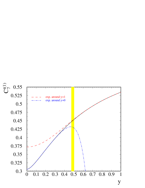
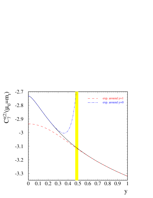
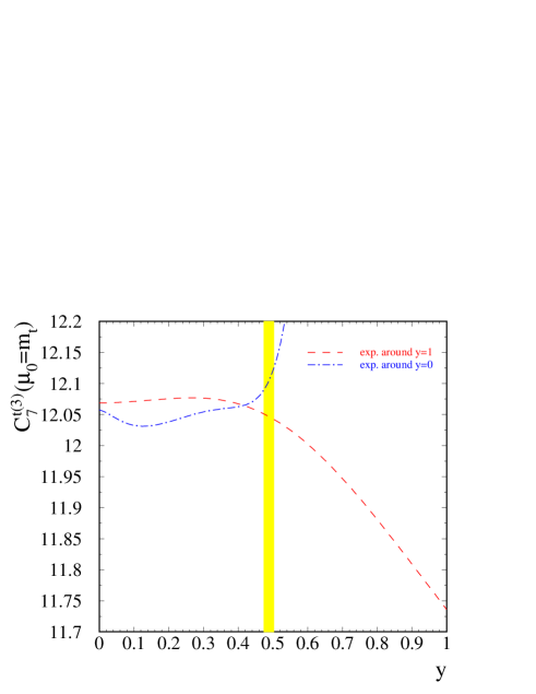
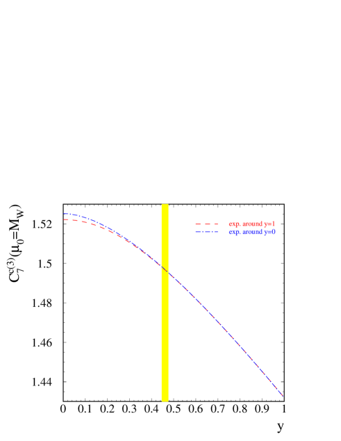
Figure 3: The coefficients $C_{7}^{Q(n)}(\mu_{0})$ as functions of $y=M_{W}/m_{t}(\mu_{0})$. The (blue) dot-dashed lines correspond to their expansions in $y$ up to $y^{8}$. The (red) dashed lines describe the expansions in $(1-y^{2})$ up to $(1-y^{2})^{8}$. The (black) solid lines in the one- and two-loop cases correspond to the known exact expressions. The (yellow) vertical strips indicate the experimental range for $y$.

In Figs. 3 and 4, the top-mass dependent coefficients $C_{i}^{t(n)}(\mu_{0}=m_{t})$ and $C_{i}^{c(3)}(\mu_{0}=M_{W})$ for $i=7,8$ are plotted as functions of $y=M_{W}/m_{t}(\mu_{0})$. The different choice of renormalization scales in the top and charm sectors allows us to avoid logarithmic divergences at large $m_{t}$ and, consequently, achieve better control over the behaviour of the expansions. This is the main reason why $\mu_{0}$ has been normalized to $M_{W}$ in the charm sector and to $m_{t}$ in the top sector, in all our intermediate and final expressions.

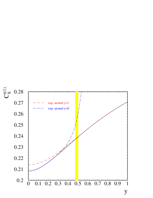
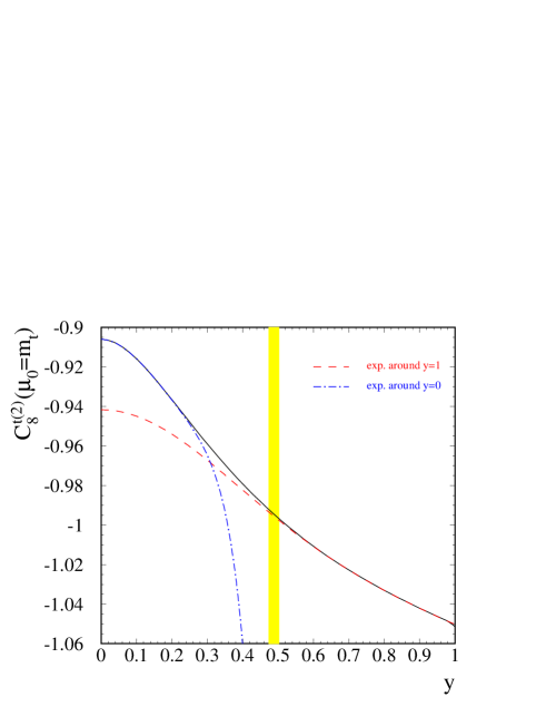
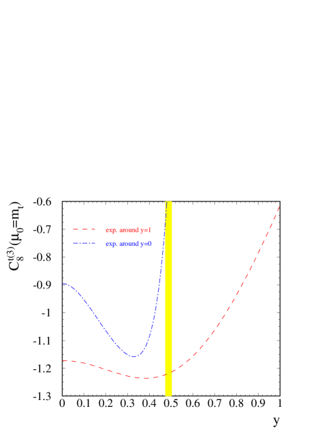
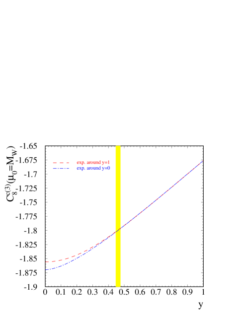
Figure 4: Same as Fig. 3 but for $C_{8}^{Q(n)}(\mu_{0})$.

The variable $y$ changes from 0 to 1, i.e. both starting points of our expansions are present in the figures. Note the relatively narrow ranges of the coefficient values on the vertical axes. The large $m_{t}$ expansions (up to $y^{8}$) are depicted by the dot-dashed lines, while the expansions around $m_{t}=M_{W}$ (up to $(1-y^{2})^{8}$) are given by the dashed ones. In the one- and two-loop cases, solid curves show the exact results. The vertical strips mark the experimental values for $y$ that we take $(0.488\pm 0.015)$ for $\mu_{0}=m_{t}$, and $(0.461\pm 0.015)$ for $\mu_{0}=M_{W}$.

Comparing the three curves in the one- and two-loop cases (the two upper plots in both figures), one can conclude that a combination of the two expansions at hand gives a good determination of the studied coefficients in the whole considered range of $y$. However, the expansion starting from $y=1$ works somewhat better for the physical values of $m_{t}$ and $M_{W}$. Most probably, including more terms in the the large $m_{t}$ expansion could improve its behaviour around $y=0.5$.

Although we do not know the exact curves in the three-loop case, the same pattern seems to repeat. In fact, the charm-sector expansions perfectly overlap in the physical region. In the top sector, one can (conservatively) conclude that

$$C_{7}^{t(3)}(\mu_{0}=m_{t}) = 12.05\pm 0.05,$$ (6.21)

$$C_{8}^{t(3)}(\mu_{0}=m_{t}) = -1.2\pm 0.1,$$ (6.22)

which is perfectly accurate for any phenomenological application. Let us note that a change of $C_{7}^{t(3)}(\mu_{0}=m_{t})$ from 12 to 13 would affect the $b\to s\gamma$ decay width by only 0.02%, while a similar variation of $C_{8}^{t(3)}(\mu_{0}=m_{t})$ would cause even a smaller effect.

For the three-loop charm-sector coefficients, the uncertainty from the expansions is smaller than the one from the experimental error in $m_{t}$. Thus, one can safely use Eqs. (6.13)–(6.16) as they stand, without any additional uncertainty. Accurate values in the range $0.4<y<0.6$ can also be found from the following fits:

$$C_{7}^{c(3)}(\mu_{0}=M_{W}) = 1.458\left(\frac{m_{t}}{M_{W}}\right)^{0.0338},$$ (6.23)

$$C_{8}^{c(3)}(\mu_{0}=M_{W}) = -1.718\left(\frac{m_{t}}{M_{W}}\right)^{0.0598}.$$ (6.24)

It is instructive to study the behaviour of the three-loop top-sector coefficients in a plot where subsequent terms of our expansions are successively taken into account. This is shown in Fig. 5.

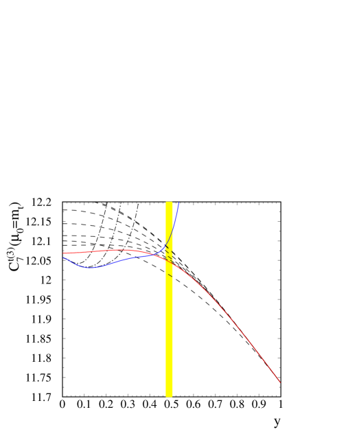
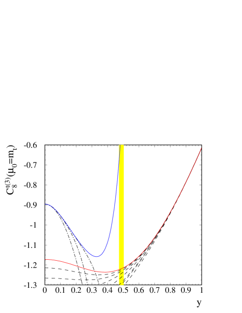
Figure 5: The three-loop top-sector coefficients. The solid lines represent the highest orders we know (as in Figs. 3 and 4). The dashed and dot-dashed lines show the lower orders.

The quality of the two expansions in various regions of $y$ is transparent there.

7 Conclusions

The three-loop matching conditions found in the present paper complete the first out of three steps (matching, mixing and matrix elements) that are necessary for finding the NNLO QCD corrections to $\bar{B}\to X_{s}\gamma$. The effect of the NNLO matching alone is scheme- and scale-dependent. In the $\overline{\rm MS}$ scheme with $M_{W}<\mu_{0}<m_{t}$, it stays within 2% of the decay width, i.e. it is significantly smaller than the total higher-order perturbative uncertainty that was estimated in Ref. [6]. This uncertainty is expected to get significantly suppressed in the near future, after the remaining two steps of the NNLO calculation are performed.

The methods that we have applied in the present work are, in principle, applicable to any three-loop matching computation involving several different mass scales. A detailed description that we have presented for each step of our procedure can serve as a guideline for treating similar problems in various domains of particle phenomenology.

Appendix A:   Three-loop expansion terms

In this appendix, we present our results for the coefficients $a_{nm}^{kQ}$ and $b_{n}^{kQ}$ from Eqs. (3.30) and (3.31) up to $n=4$ and $n=8$, respectively. They are given in terms of the following symbols (see also Eq. (16) of Ref. [13]):

$$D_{3} = 6\zeta_{3}-\frac{15}{4}\zeta_{4}-6\left[\mbox{Cl}_{2}\left(\frac{\pi}{3}\right)\right]^{2}\,,$$

$$B_{4} = -4\zeta_{2}\ln^{2}2+\frac{2}{3}\ln^{4}2-\frac{13}{2}\zeta_{4}+16\mbox{Li}_{4}\left(\frac{1}{2}\right)\,,$$

$$S_{2} = \frac{4}{9\sqrt{3}}\mbox{Cl}_{2}\left(\frac{\pi}{3}\right)\,,$$

$$S_{2}^{\varepsilon} = -\frac{763}{32}-\frac{9\pi\sqrt{3}\ln^{2}3}{16}-\frac{35\pi^{3}\sqrt{3}}{48}+\frac{195}{16}\zeta_{2}-\frac{15}{4}\zeta_{3}+\frac{57}{16}\zeta_{4}$$

$$\mbox{}+\frac{45\sqrt{3}}{2}{\rm Cl}_{2}\left(\frac{\pi}{3}\right)-27\sqrt{3}{\rm Im}\left[{\rm Li}_{3}\left(\frac{e^{-i\pi/6}}{\sqrt{3}}\right)\right]\,,$$

$$T_{1}^{\varepsilon} = -\frac{45}{2}-\frac{\pi\sqrt{3}\ln^{2}3}{8}$$ (A.1)

$$\mbox{}-\frac{35\pi^{3}\sqrt{3}}{216}-\frac{9}{2}\zeta_{2}+\zeta_{3}+6\sqrt{3}{\rm Cl}_{2}\left(\frac{\pi}{3}\right)-6\sqrt{3}{\rm Im}\left[{\rm Li}_{3}\left(\frac{e^{-i\pi/6}}{\sqrt{3}}\right)\right]\,,$$

where ${\rm Cl}_{2}(x)={\rm Im}\left[{\rm Li}_{2}\left(e^{ix}\right)\right]$.

The expansion coefficients that we have found read

$$a_{00}^{7t} = +{\textstyle\frac{70\zeta(3)}{243}}+{\textstyle\frac{1587S_{2}}{280}}+{\textstyle\frac{43\pi^{4}}{405}}+{\textstyle\frac{416341\pi^{2}}{612360}}+{\textstyle\frac{46D_{3}}{81}}-{\textstyle\frac{92B_{4}}{81}}+{\textstyle\frac{820640533}{9185400}}\,,$$

$$a_{10}^{7t} = +{\textstyle\frac{307721\zeta(3)}{324}}-{\textstyle\frac{67T_{1}^{\varepsilon}}{18}}-{\textstyle\frac{284327S_{2}}{840}}+{\textstyle\frac{96959\pi^{4}}{116640}}-{\textstyle\frac{53880251\pi^{2}}{816480}}+{\textstyle\frac{67S_{2}^{\varepsilon}}{27}}+{\textstyle\frac{680D_{3}}{81}}-{\textstyle\frac{1360B_{4}}{81}}-{\textstyle\frac{2469729799}{4082400}}\,,$$

$$a_{11}^{7t} = -{\textstyle\frac{201S_{2}}{4}}+{\textstyle\frac{49\pi^{2}}{54}}-{\textstyle\frac{2669}{810}}\,,$$

$$a_{12}^{7t} = -{\textstyle\frac{11}{6}}\,,$$

$$a_{13}^{7t} = -{\textstyle\frac{19}{18}}\,,$$

$$a_{20}^{7t} = +{\textstyle\frac{138245\zeta(3)}{54}}-{\textstyle\frac{4073T_{1}^{\varepsilon}}{81}}-{\textstyle\frac{333063S_{2}}{140}}+{\textstyle\frac{122821\pi^{4}}{58320}}-{\textstyle\frac{7316857\pi^{2}}{81648}}+{\textstyle\frac{8146S_{2}^{\varepsilon}}{243}}+34D_{3}-68B_{4}-{\textstyle\frac{1981904129}{408240}}\,,$$

$$a_{21}^{7t} = -{\textstyle\frac{4073S_{2}}{6}}+{\textstyle\frac{3943\pi^{2}}{162}}+{\textstyle\frac{306769}{1215}}\,,$$

$$a_{22}^{7t} = +{\textstyle\frac{4613}{81}}\,,$$

$$a_{23}^{7t} = +{\textstyle\frac{146}{27}}\,,$$

$$a_{30}^{7t} = +{\textstyle\frac{138120863\zeta(3)}{26244}}-{\textstyle\frac{3547685T_{1}^{\varepsilon}}{13122}}-{\textstyle\frac{98842253S_{2}}{9720}}+{\textstyle\frac{17476801\pi^{4}}{9447840}}+{\textstyle\frac{284448283\pi^{2}}{3149280}}+{\textstyle\frac{3547685S_{2}^{\varepsilon}}{19683}}$$

$$\hskip 256.0748pt+{\textstyle\frac{7432D_{3}}{81}}-{\textstyle\frac{14864B_{4}}{81}}-{\textstyle\frac{32458492807}{1574640}}\,,$$

$$a_{31}^{7t} = -{\textstyle\frac{3547685S_{2}}{972}}+{\textstyle\frac{506753\pi^{2}}{2916}}+{\textstyle\frac{46342189}{17496}}\,,$$

$$a_{32}^{7t} = +{\textstyle\frac{1751809}{2916}}\,,$$

$$a_{33}^{7t} = +{\textstyle\frac{251}{3}}\,,$$

$$a_{40}^{7t} = +{\textstyle\frac{257322953\zeta(3)}{26244}}-{\textstyle\frac{12491099T_{1}^{\varepsilon}}{13122}}-{\textstyle\frac{5628051553S_{2}}{174960}}-{\textstyle\frac{54918881\pi^{4}}{9447840}}+{\textstyle\frac{12685755337\pi^{2}}{22044960}}+{\textstyle\frac{12491099S_{2}^{\varepsilon}}{19683}}$$

$$\hskip 256.0748pt+{\textstyle\frac{16166D_{3}}{81}}-{\textstyle\frac{32332B_{4}}{81}}-{\textstyle\frac{190409709691}{3149280}}\,,$$

$$a_{41}^{7t} = -{\textstyle\frac{12491099S_{2}}{972}}+{\textstyle\frac{1978619\pi^{2}}{2916}}+{\textstyle\frac{531316991}{43740}}\,,$$

$$a_{42}^{7t} = +{\textstyle\frac{664799}{243}}\,,$$

$$a_{43}^{7t} = +{\textstyle\frac{3424}{9}}\,,$$ (A.2)

$$b_{0}^{7t} = -{\textstyle\frac{2901893\zeta(3)}{38880}}+{\textstyle\frac{4909\pi^{2}}{2160}}+{\textstyle\frac{1797615371}{8748000}}\,,$$

$$b_{1}^{7t} = +{\textstyle\frac{94143997\zeta(3)}{1244160}}-{\textstyle\frac{6763\pi^{2}}{15120}}-{\textstyle\frac{113487750073}{979776000}}\,,$$

$$b_{2}^{7t} = +{\textstyle\frac{91942073\zeta(3)}{860160}}-{\textstyle\frac{241\pi^{2}}{1512}}-{\textstyle\frac{10092619036343}{76814438400}}\,,$$

$$b_{3}^{7t} = +{\textstyle\frac{137418234607\zeta(3)}{891813888}}-{\textstyle\frac{8\pi^{2}}{135}}-{\textstyle\frac{13709395882765691}{73741860864000}}\,,$$

$$b_{4}^{7t} = +{\textstyle\frac{7490373009073\zeta(3)}{35672555520}}-{\textstyle\frac{593\pi^{2}}{30240}}-{\textstyle\frac{5960644239577417}{23597395476480}}\,,$$

$$b_{5}^{7t} = +{\textstyle\frac{467301421361\zeta(3)}{1698693120}}-{\textstyle\frac{131\pi^{2}}{47520}}-{\textstyle\frac{6438103242654889429}{19467851268096000}}\,,$$

$$b_{6}^{7t} = +{\textstyle\frac{329068267226885\zeta(3)}{941755465728}}+{\textstyle\frac{1139\pi^{2}}{249480}}-{\textstyle\frac{1798715398515135307759}{4282927278981120000}}\,,$$

$$b_{7}^{7t} = +{\textstyle\frac{1164930029277053\zeta(3)}{2690729902080}}+{\textstyle\frac{353\pi^{2}}{46332}}-{\textstyle\frac{445971686554467633047}{857084922534297600}}\,,$$

$$b_{8}^{7t} = +{\textstyle\frac{32688338029429333\zeta(3)}{62185757736960}}+{\textstyle\frac{56293\pi^{2}}{6486480}}-{\textstyle\frac{12555120069922446322011879253}{19873056681818251591680000}}\,,$$ (A.3)

$$a_{00}^{8t} = -{\textstyle\frac{22301\zeta(3)}{648}}+{\textstyle\frac{22149S_{2}}{224}}+{\textstyle\frac{17\pi^{4}}{2160}}+{\textstyle\frac{170659\pi^{2}}{25515}}+{\textstyle\frac{13D_{3}}{216}}-{\textstyle\frac{13B_{4}}{108}}+{\textstyle\frac{1189623529}{61236000}}\,,$$

$$a_{10}^{8t} = -{\textstyle\frac{147193\zeta(3)}{432}}+{\textstyle\frac{1075273S_{2}}{2240}}-{\textstyle\frac{1733\pi^{4}}{2430}}+{\textstyle\frac{3172381\pi^{2}}{544320}}-{\textstyle\frac{56D_{3}}{27}}+{\textstyle\frac{112B_{4}}{27}}+{\textstyle\frac{409119733}{1360800}}\,,$$

$$a_{11}^{8t} = -{\textstyle\frac{581}{5400}}\,,$$

$$a_{12}^{8t} = -{\textstyle\frac{1}{80}}\,,$$

$$a_{20}^{8t} = -{\textstyle\frac{304559\zeta(3)}{216}}+{\textstyle\frac{49T_{1}^{\varepsilon}}{2}}+{\textstyle\frac{3422759S_{2}}{1920}}-{\textstyle\frac{9289\pi^{4}}{4320}}+{\textstyle\frac{271907\pi^{2}}{31104}}-{\textstyle\frac{49S_{2}^{\varepsilon}}{3}}-{\textstyle\frac{349D_{3}}{24}}+{\textstyle\frac{349B_{4}}{12}}+{\textstyle\frac{487461187}{155520}}\,,$$

$$a_{21}^{8t} = +{\textstyle\frac{1323S_{2}}{4}}-{\textstyle\frac{3811\pi^{2}}{432}}-{\textstyle\frac{8187697}{64800}}\,,$$

$$a_{22}^{8t} = -{\textstyle\frac{63517}{2160}}\,,$$

$$a_{23}^{8t} = -{\textstyle\frac{199}{72}}\,,$$

$$a_{30}^{8t} = -{\textstyle\frac{8128418\zeta(3)}{2187}}+{\textstyle\frac{3891425T_{1}^{\varepsilon}}{17496}}+{\textstyle\frac{284508347S_{2}}{36288}}-{\textstyle\frac{26167261\pi^{4}}{12597120}}+{\textstyle\frac{115972585\pi^{2}}{5878656}}-{\textstyle\frac{3891425S_{2}^{\varepsilon}}{26244}}$$

$$\hskip 256.0748pt-{\textstyle\frac{6097D_{3}}{108}}+{\textstyle\frac{6097B_{4}}{54}}+{\textstyle\frac{255386869021}{14696640}}\,,$$

$$a_{31}^{8t} = +{\textstyle\frac{3891425S_{2}}{1296}}-{\textstyle\frac{442091\pi^{2}}{3888}}-{\textstyle\frac{1407902803}{583200}}\,,$$

$$a_{32}^{8t} = -{\textstyle\frac{10526363}{19440}}\,,$$

$$a_{33}^{8t} = -{\textstyle\frac{117}{2}}\,,$$

$$a_{40}^{8t} = -{\textstyle\frac{1201430399\zeta(3)}{139968}}+{\textstyle\frac{72196517T_{1}^{\varepsilon}}{69984}}+{\textstyle\frac{28165051597S_{2}}{933120}}+{\textstyle\frac{83544979\pi^{4}}{10077696}}+{\textstyle\frac{33972092933\pi^{2}}{117573120}}-{\textstyle\frac{72196517S_{2}^{\varepsilon}}{104976}}$$

$$\hskip 256.0748pt-{\textstyle\frac{34039D_{3}}{216}}+{\textstyle\frac{34039B_{4}}{108}}+{\textstyle\frac{206714107565}{3359232}}\,,$$

$$a_{41}^{8t} = +{\textstyle\frac{72196517S_{2}}{5184}}-{\textstyle\frac{9280985\pi^{2}}{15552}}-{\textstyle\frac{4347341779}{291600}}\,,$$

$$a_{42}^{8t} = -{\textstyle\frac{20676181}{6480}}\,,$$

$$a_{43}^{8t} = -{\textstyle\frac{1379}{4}}\,,$$ (A.4)

$$b_{0}^{8t} = -{\textstyle\frac{3426427\zeta(3)}{207360}}+{\textstyle\frac{4007\pi^{2}}{2880}}+{\textstyle\frac{383324521}{4665600}}\,,$$

$$b_{1}^{8t} = +{\textstyle\frac{377401\zeta(3)}{12960}}-{\textstyle\frac{901\pi^{2}}{10080}}-{\textstyle\frac{683934529}{16329600}}\,,$$

$$b_{2}^{8t} = +{\textstyle\frac{257020361\zeta(3)}{3870720}}+{\textstyle\frac{247\pi^{2}}{20160}}-{\textstyle\frac{5133539931187}{64012032000}}\,,$$

$$b_{3}^{8t} = +{\textstyle\frac{148678249549\zeta(3)}{1486356480}}+{\textstyle\frac{25\pi^{2}}{1008}}-{\textstyle\frac{590349164605337}{4916124057600}}\,,$$

$$b_{4}^{8t} = +{\textstyle\frac{48644809387\zeta(3)}{339738624}}+{\textstyle\frac{869\pi^{2}}{40320}}-{\textstyle\frac{33797460512670161}{196644962304000}}\,,$$

$$b_{5}^{8t} = +{\textstyle\frac{3067923823757\zeta(3)}{15854469120}}+{\textstyle\frac{3649\pi^{2}}{221760}}-{\textstyle\frac{6031703724292608407}{25957135024128000}}\,,$$

$$b_{6}^{8t} = +{\textstyle\frac{787852603809259\zeta(3)}{3139184885760}}+{\textstyle\frac{16189\pi^{2}}{1330560}}-{\textstyle\frac{9469141155025123085807}{31408133379194880000}}\,,$$

$$b_{7}^{8t} = +{\textstyle\frac{113217484992547\zeta(3)}{358763986944}}+{\textstyle\frac{173\pi^{2}}{19305}}-{\textstyle\frac{1857857271774679586364179}{4899668807154401280000}}\,,$$

$$b_{8}^{8t} = +{\textstyle\frac{96339777793582171\zeta(3)}{248743030947840}}+{\textstyle\frac{11485\pi^{2}}{1729728}}-{\textstyle\frac{948680668305509273934263213}{2038262223776230932480000}}\,,$$ (A.5)

$$a_{00}^{7c} = -{\textstyle\frac{5032\zeta(3)}{243}}+{\textstyle\frac{29683\pi^{2}}{4374}}-{\textstyle\frac{517861}{39366}}\,,$$

$$a_{01}^{7c} = +{\textstyle\frac{407}{729}}\,,$$

$$a_{02}^{7c} = -{\textstyle\frac{112}{243}}\,,$$

$$a_{10}^{7c} = -{\textstyle\frac{112}{1215}}\,,$$

$$a_{11}^{7c} = +{\textstyle\frac{8}{405}}\,,$$

$$a_{20}^{7c} = +{\textstyle\frac{19\pi^{2}}{5670}}+{\textstyle\frac{4960261}{166698000}}\,,$$

$$a_{21}^{7c} = -{\textstyle\frac{2123}{396900}}\,,$$

$$a_{22}^{7c} = +{\textstyle\frac{19}{1890}}\,,$$

$$a_{30}^{7c} = -{\textstyle\frac{4\pi^{2}}{3645}}-{\textstyle\frac{752008}{24111675}}\,,$$

$$a_{31}^{7c} = -{\textstyle\frac{5876}{382725}}\,,$$

$$a_{32}^{7c} = -{\textstyle\frac{4}{1215}}\,,$$

$$a_{40}^{7c} = +{\textstyle\frac{3075421}{1296672300}}\,,$$

$$a_{41}^{7c} = +{\textstyle\frac{74}{93555}}\,,$$ (A.6)

$$b_{0}^{7c} = -{\textstyle\frac{7048\zeta(3)}{243}}-{\textstyle\frac{69S_{2}}{14}}+{\textstyle\frac{103925\pi^{2}}{15309}}-{\textstyle\frac{6854384}{3444525}}\,,$$

$$b_{1}^{7c} = -{\textstyle\frac{448\zeta(3)}{27}}+{\textstyle\frac{653S_{2}}{35}}-{\textstyle\frac{29\pi^{2}}{8505}}+{\textstyle\frac{670214}{42525}}\,,$$

$$b_{2}^{7c} = -{\textstyle\frac{224\zeta(3)}{9}}+{\textstyle\frac{10109S_{2}}{210}}+{\textstyle\frac{\pi^{2}}{17010}}+{\textstyle\frac{16246}{945}}\,,$$

$$b_{3}^{7c} = -{\textstyle\frac{896\zeta(3)}{27}}+{\textstyle\frac{3676S_{2}}{45}}+{\textstyle\frac{4\pi^{2}}{3645}}+{\textstyle\frac{7423}{405}}\,,$$

$$b_{4}^{7c} = -{\textstyle\frac{1120\zeta(3)}{27}}+{\textstyle\frac{3166S_{2}}{27}}+{\textstyle\frac{92539}{4860}}\,,$$

$$b_{5}^{7c} = -{\textstyle\frac{448\zeta(3)}{9}}+{\textstyle\frac{62512S_{2}}{405}}+{\textstyle\frac{352919}{18225}}\,,$$

$$b_{6}^{7c} = -{\textstyle\frac{1568\zeta(3)}{27}}+{\textstyle\frac{5200S_{2}}{27}}+{\textstyle\frac{235619}{12150}}\,,$$

$$b_{7}^{7c} = -{\textstyle\frac{1792\zeta(3)}{27}}+{\textstyle\frac{1970884S_{2}}{8505}}+{\textstyle\frac{1468651}{76545}}\,,$$

$$b_{8}^{7c} = -{\textstyle\frac{224\zeta(3)}{3}}+{\textstyle\frac{13859809S_{2}}{51030}}+{\textstyle\frac{6903803}{367416}}\,,$$ (A.7)

$$a_{00}^{8c} = -{\textstyle\frac{1627\zeta(3)}{162}}+{\textstyle\frac{25583\pi^{2}}{5832}}+{\textstyle\frac{9148337}{104976}}\,,$$

$$a_{01}^{8c} = +{\textstyle\frac{1049}{486}}\,,$$

$$a_{02}^{8c} = -{\textstyle\frac{23}{81}}\,,$$

$$a_{10}^{8c} = +{\textstyle\frac{9707}{32400}}\,,$$

$$a_{11}^{8c} = +{\textstyle\frac{601}{2160}}\,,$$

$$a_{20}^{8c} = +{\textstyle\frac{29\pi^{2}}{7560}}+{\textstyle\frac{462793}{6945750}}\,,$$

$$a_{21}^{8c} = +{\textstyle\frac{2479}{66150}}\,,$$

$$a_{22}^{8c} = +{\textstyle\frac{29}{2520}}\,,$$

$$a_{30}^{8c} = +{\textstyle\frac{11\pi^{2}}{108864}}-{\textstyle\frac{1616438903}{144027072000}}\,,$$

$$a_{31}^{8c} = -{\textstyle\frac{496373}{114307200}}\,,$$

$$a_{32}^{8c} = +{\textstyle\frac{11}{36288}}\,,$$

$$a_{40}^{8c} = -{\textstyle\frac{13282901}{8644482000}}\,,$$

$$a_{41}^{8c} = -{\textstyle\frac{1879}{2494800}}\,,$$ (A.8)

$$b_{0}^{8c} = -{\textstyle\frac{2833\zeta(3)}{162}}-{\textstyle\frac{29871S_{2}}{2240}}+{\textstyle\frac{7169669\pi^{2}}{1632960}}+{\textstyle\frac{7342571207}{73483200}}\,,$$

$$b_{1}^{8c} = -{\textstyle\frac{131\zeta(3)}{9}}+{\textstyle\frac{597S_{2}}{2240}}-{\textstyle\frac{1447\pi^{2}}{181440}}+{\textstyle\frac{17694343}{907200}}\,,$$

$$b_{2}^{8c} = -{\textstyle\frac{65\zeta(3)}{3}}+{\textstyle\frac{50339S_{2}}{2240}}+{\textstyle\frac{751\pi^{2}}{181440}}+{\textstyle\frac{1260331}{60480}}\,,$$

$$b_{3}^{8c} = -{\textstyle\frac{259\zeta(3)}{9}}+{\textstyle\frac{64417S_{2}}{1344}}-{\textstyle\frac{11\pi^{2}}{108864}}+{\textstyle\frac{4083773}{181440}}\,,$$

$$b_{4}^{8c} = -{\textstyle\frac{323\zeta(3)}{9}}+{\textstyle\frac{10871S_{2}}{144}}+{\textstyle\frac{307651}{12960}}\,,$$

$$b_{5}^{8c} = -43\zeta(3)+{\textstyle\frac{45223S_{2}}{432}}+{\textstyle\frac{4783799}{194400}}\,,$$

$$b_{6}^{8c} = -{\textstyle\frac{451\zeta(3)}{9}}+{\textstyle\frac{2431S_{2}}{18}}+{\textstyle\frac{816431}{32400}}\,,$$

$$b_{7}^{8c} = -{\textstyle\frac{515\zeta(3)}{9}}+{\textstyle\frac{3773167S_{2}}{22680}}+{\textstyle\frac{10434863}{408240}}\,,$$

$$b_{8}^{8c} = -{\textstyle\frac{193\zeta(3)}{3}}+{\textstyle\frac{108012589S_{2}}{544320}}+{\textstyle\frac{252135383}{9797760}}\,.$$ (A.9)

References

[1]
S. Chen et al. (CLEO Collaboration),
Phys. Rev. Lett. 87 (2001) 251807
[hep-ex/0108032].
[2]
R. Barate et al. (ALEPH Collaboration),
Phys. Lett. B 429 (1998) 169.
[3]
K. Abe et al. (BELLE Collaboration),
Phys. Lett. B 511 (2001) 151
[hep-ex/0103042].
[4]
B. Aubert et al. (BABAR Collaboration),
[hep-ex/0207076].
[5] C. Jessop, SLAC report SLAC-PUB-9610, November 2002.
[6]
P. Gambino and M. Misiak,
Nucl. Phys. B 611 (2001) 338
[hep-ph/0104034].
[7]
A.J. Buras, A. Czarnecki, M. Misiak and J. Urban,
Nucl. Phys. B 631 (2002) 219
[hep-ph/0203135].
[8]
C. Greub, T. Hurth and D. Wyler,
Phys. Rev. D 54 (1996) 3350
[hep-ph/9603404].
[9]
C. Bobeth, M. Misiak and J. Urban,
Nucl. Phys. B 574 (2000) 291
[hep-ph/9910220].
[10]
A. J. Buras and M. Misiak,
Acta Phys. Pol. B 33 (2002) 2597
[hep-ph/0207131].
[11]
K. Bieri, C. Greub and M. Steinhauser,
Phys. Rev. D 67 (2003) 114019
[hep-ph/0302051].
[12] P. Gambino, M. Gorbahn and U. Haisch, in preparation.
[13]
M. Steinhauser,
Comput. Phys. Commun. 134 (2001) 335
[hep-ph/0009029].
[14]
K.G. Chetyrkin, M. Misiak and M. Münz,
Phys. Lett. B 400 (1997) 206,
Phys. Lett. B 425 (1998) 414 (E)
[hep-ph/9612313].
[15]
P. Gambino, M. Gorbahn and U. Haisch,
Nucl. Phys. B 673 (2003) 238
[hep-ph/0306079].
[16]
B. Grinstein, R. P. Springer and M. B. Wise,
Nucl. Phys. B 339 (1990) 269.
[17]
V. A. Smirnov,
Applied Asymptotic Expansions in Momenta and Masses,
Springer-Verlag, Heidelberg, 2001.
[18]
P. Nogueira,
J. Comp. Phys. 105 (1993) 279.
[19]
T. Seidensticker, unpublished.
[20]
T. Seidensticker,
hep-ph/9905298;
R. Harlander, T. Seidensticker and M. Steinhauser,
Phys. Lett. B 426 (1998) 125
[hep-ph/9712228].
[22]
J. Küblbeck, M. Böhm and A. Denner,
Comput. Phys. Commun. 60 (1990) 165;
T. Hahn and C. Schappacher,
Comput. Phys. Commun. 143 (2002) 54
[hep-ph/0105349].
[23]
M. Steinhauser,
Phys. Rept. 364 (2002) 247
[hep-ph/0201075].