Meson-Baryon Couplings from QCD Sum Rules

Abstract

Coupling constants of the pseudoscalar mesons to the octet baryons are calculated in the QCD sum rule approach. Two-point correlation function of the baryons are evaluated in a single meson state and the vacuum, which yields the designated coupling. The emphasis is on the flavor SU(3) structure of the coupling constants and reliability in extracting the coupling constants from the two-point correlation functions. We first calculate the baryon-diagonal couplings and study the reliability of the sum rule. The $F/D$ ratio of the coupling is determined in the SU(3) limit. We further formulate the baryon-off-diagonal couplings using the projected correlation functions and the vertex functions, so that the unwanted excited states do not contaminate the sum rule. As an example, the $\pi\Lambda\Sigma$ coupling constant is calculated and the flavor SU(3) breaking effect is studied. We find that the effect of SU(3) breaking on the $\pi\Lambda\Sigma$ coupling constant is small.

I introduction

Quantum chromodynamics (QCD) has overwhelming evidences as the right theory of strong interactions of quarks and gluons. It successfully describes hard processes of hadrons, such as the scaling behaviors of structure functions, and the positron-electron annihilation cross sections PDG-QCD . The lattice QCD gives nonperturbative properties of the vacuum, such as color confinement, quark condensate and so on, which are consistent with properties of low lying hadrons. Some (but not all) properties of hadrons, i.e., masses, are now available directly from lattice QCD LQCD-conf . QCD also suggests fascinating possibility of phase transitions of the vacuum at finite temperature and/or baryon density QCD-finiteT . A dedicated accelerator has just begun to look for evidences of such phase transition RHIC .

On the other hand, applications of QCD to rich phenomena of low energy hadrons are not in bloom yet. So far, hadronic interactions have been studied mostly in phenomenological approaches. The most prominent example is the nuclear force. State-of-art $N-N$ potentials, which are valid to relatively high energy ($\sim 1$ GeV) , are available in the market NNpot ; Nijmegen . They are based on the meson exchange picture, which has been developed in these fifty years since Yukawa proposed the pion exchange interaction Yukawa , and phenomenological short-range part, which should be attributed to the dynamics of quarks and gluons inside the baryon QCM-ptp . Although it is highly desirable to establish a foundation of such potentials from the QCD viewpoint, no immediate resolution is expected at this moment.

Recent development of hypernuclear physics has lead us to the level that the interactions of hyperons, $\Lambda$, $\Sigma$, $\Xi$, and so on (collectively denoted by $Y$), can be fairly well studied from the observed spectra of hypernuclei as well as the data from hyperon productions and reactions Hyper2000 . It has been found that the $\Lambda-N$ interaction is somewhat weaker than the $N-N$ interaction, and its spin dependent part has new features ALS-oka . The $Y-N$ interaction is naturally regarded as a generalized nuclear force by including the third flavor, strangeness YN-SU3 . Thus, we consider a larger flavor space, i.e., the flavor SU(3). In terms of SU(3) , the systems composed of two octet baryons belong to

$$8\times 8=1+8_{s}+27+8_{a}+10+\overline{10}$$

irreducible representations. Among them the first (last) three are symmetric (antisymmetric) under the exchange of two baryons, and therefore appear in the channels with antisymmetric (symmetric) spin-orbital combination. The $N-N$ systems have the hypercharge $Y=B+S=+2$ and thus belong to either 27 or $\overline{10}$ representation. In other words, all the other representations are not accessible by $N-N$, but can be reachable only by $Y-N$ and $Y-Y$ interactions. In this sense, study of the $Y-N$ and $Y-Y$ interactions is important for the complete understanding of the baryonic interactions.

Theoretical approaches to the $Y-N$ interaction are naturally to generalize the picture of the $N-N$ interaction by considering exchanges of the pseudoscalar octet, the vector octet as well as the singlet pseudoscalar and vector mesons. Again the short-range parts of the potential are given phenomenologically. Much efforts have been made to analyze experimental data to draw a consistent picture of the hyperon interactions. Yet the the most fundamental quantities, i.e., the meson-baryon coupling constants, which are essential in constructing the meson exchange forces of baryons, have been treated as unknown parameters. In order to reduce the ambiguity, the SU(3) relations of the coupling constants are often employed, which leaves a free parameter, i.e., the $F/D$ ratio. A very popular phenomenological $Y-N$ potential is the Nijmegen model Nijmegen , which has several different versions. There the $F/D$ ratio is treated as a free parameter and varies among the different versions. However, the effect of SU(3) breaking may well be sizable considering a wide variety of meson masses within the octet Lutz .

Under these circumstances, it is highly desirable to calculate the meson-baryon coupling constants from the fundamental theory. What is the $F/D$ ratio in the SU(3) limit? How is the SU(3) symmetry broken at the meson-baryon vertices? A lattice QCD calculation may be preferable, but at this moment is still preliminary LQCDpiNN . Thus alternative analytic approaches may be useful to analyze the SU(3) symmetry structure of the couplings.

In this paper, we employ QCD sum rule approach to the coupling constants of the pseudoscalar octet mesons and the octet baryons. The QCD sum rule SVZ ; RRY is generally a relation derived from a correlation function in QCD and its analytic property. The correlation function is calculated by the use of operator product expansion (OPE) in the deeply Euclidean region on one hand, and is compared with that calculated for a phenomenological parameterization. The sum rules relate hadron properties directly to the QCD vacuum condensates as well as the other fundamental constants. Most applications consider two-point correlation functions of hadronic interpolating operators, and derive relations of masses and other single-particle properties of the designated hadron (ex. Ioffe ). It has been applied to the properties of hadrons at finite temperature and density QCDSR-finiteTrho , as well as the calculation of the scattering lengths of two hadrons QCDSRNN . The obtained sum rules generally give predictions up to a few tens of per cent ambiguity, which may come from ambiguities of the QCD parameters as well as higher orders in OPE truncation and contaminations from excited and continuum states.

Application of the sum rule to the meson-baryon coupling constants, (mostly the $\pi NN$ coupling constant), was started by Reinders et al. Reinders ; RRY2 , who pointed out that the use of three point functions results in $g_{\pi NN}$ which is inconsistent with the Goldberger-Treiman (GT) relation. They then considered two-point correlation function with the pion in the initial state,

$$\Pi^{\alpha\beta}(q,p)=i\int d^{4}x\,e^{iq\cdot x}\langle 0|{\rm T}\left[J^{\alpha}_{N}(x)\bar{J}^{\beta}_{N}(0)\right]|\pi(p)\rangle$$ (1)

and showed that the sum rule for the first nonperturbative term in OPE gives the GT relation with $g_{A}=1$. Later, Shiomi and Hatsuda SH improved the sum rule in the soft-pion limit ($p\to 0$) including higher orders in the OPE. However, Birse and Krippa BK1 pointed out that the sum rule at $p\to 0$ simply reflects the result of the GT relation and does not constitute an independent sum rule from that for the nucleon mass. It can be easily shown that the correlation function (1) is related to the correlation function without the pion in the initial state using the soft pion reduction formula. Therefore in order to obtain an independent sum rule, we need to take into account finite pion momentum $p$.

As the correlation function (1) has the Dirac indices ($\alpha,\beta$), it has several independent terms, which give independent sum rules. Kim, Lee and Oka KLO investigated dependencies on the Dirac structure and suggested that the tensor (T) structure, proportional to $\gamma_{5}\sigma^{\mu\nu}q_{\mu}p_{\nu}$, gives the most reliable result. This conclusion was further refined by Kim, Doi, Oka and Lee KD1 ; DK1 . The latter also checked dependencies on the choice of the interpolating field operator for the nucleon. They found that this point is especially important in deriving the $F/D$ ratio of the coupling constants, when the formulation is extended to the SU(3) case. Recently, Kondo and Morimatsu proposed a novel construction of the sum rule using projected two-point correlation functions KM1 ; KM2 , and showed that the coupling constant can be defined without the ambiguity from the choice of the effective interaction Lagrangian.

The organization of this article is as follows. We first review the formulation of the QCD sum rule for the meson-baryon coupling constant in section II, summarizing the arguments given in Refs. DK1 ; DK2 . In section III, we formulate the sum rules for the “baryon-diagonal” coupling constants, such as $\pi NN$, $\eta NN$, $\pi\Sigma\Sigma$ and so on, and analyze their SU(3) structure. In the SU(3) limit, these couplings are related with each other. More specifically, the ratios of any two couplings are parametrized by a single common parameter, the $F/D$ ratio. As the $F/D$ ratio parametrize two allowed octet combinations in the coupling, it cannot be determined by the SU(3) symmetry alone, while requiring a larger symmetry, such as the SU(6) symmetry of the nonrelativistic quark model, determines the ratio uniquely.

In the potential model approaches Nijmegen , the $F/D$ ratio for each exchanged meson octet is considered as a free parameter, although it is often fixed to the value taken from the SU(6) symmetry, or the value determined by the semileptonic decays of hyperons. The latter provides us with the $F/D$ ratio for the axialvector charges of the baryons, and thus one has to rely on the GT relation to apply it to the $F/D$ ratio of the coupling constants. Clearly it is desirable to determine the $F/D$ ratio of the meson-baryon coupling constants directly from QCD only with the constraint of the SU(3) symmetry. Moreover, a careful study of the applicability of the sum rules in the SU(3) limit will give us confidence on the sum rule analysis when the SU(3) symmetry is broken, which is a subject of section IV.

The projected two-point correlation functions, proposed in Refs. KM1 ; KM2 can be applied to general meson-baryon couplings including the baryon-off-diagonal cases. In section IV, we take the $\pi\Lambda\Sigma$ coupling as an example and explain the projected correlation method and evaluate the sum rule for the $\pi\Lambda\Sigma$ coupling constant. We also study effects of the SU(3) breaking on this coupling constant.

We give a conclusion in section V.

II Sum rules for meson-baryon coupling constants

Reinders, Rubinstein and Yazaki, in their celebrated Physics Reports articleRRY , summarized their pioneering works on the QCD sum rules. They studied how the masses of various mesons and baryons are determined directly from QCD with the help of dispersion relation which connects operator product expansion (OPE) of QCD operators in the deep Euclidean region, which gives the OPE side of the sum rule, and the realistic spectral function at the on-mass-shell region, which gives the phenomenological side. The OPE side contains information of nonperturbative nature of QCD in terms of matrix elements, or condensates, of various local operators, such as $\langle\bar{q}q\rangle$ and $\langle\frac{\alpha_{s}}{\pi}G_{\mu\nu}G^{\mu\nu}\rangle$.

They also considered how the $\pi NN$ coupling constant is calculated in the QCD sum rule approach. They studied two correlation functions for the sum rule, the three-point correlation function Reinders ; RRY2 ,

$$\Pi(q,q^{\prime},p)=\int d^{4}xe^{iq^{\prime}x}\int d^{4}ye^{-ipy}\langle 0|{\rm T}[J_{B_{1}}(x)J_{m}(y)\bar{J}_{B_{2}}(0)]|0\rangle,$$ (2)

and the two-point correlation function with an external meson field Reinders ,

$$\Pi(q,p)=i\int d^{4}x\ e^{iq\cdot x}\langle 0|{\rm T}[J_{B_{1}}(x)\bar{J}_{B_{2}}(0)]|m(p)\rangle,$$ (3)

where $p$ is the momentum of the meson $m$. $J_{B_{1}}$ and $J_{B_{2}}$ denote local operators which interpolate the QCD vacuum and the baryon states, $B_{1}$ and $B_{2}$, respectively. $J_{m}$ is a similar operator for the meson $m$. They are called either interpolating field or “current”.

In principle, both the above correlation functions can be used to construct a sum rule for the coupling constant. However, in practice, the three-point correlation function has disadvantages that one has to assume the meson pole dominance and neglect the contribution from higher excited states. This assumption is not justified because the OPE is valid only in the deep Euclidean region of the meson momentum ($p^{2}\rightarrow-\infty$). It was demonstrated, indeed, by Maltman maltman that the sum rule for the $\pi NN$ coupling has large contamination from the excited pions, $\pi(1300)$ and $\pi(1800)$. On the other hand, for the two-point correlation function, we may take into account the relevant meson exclusively via the corresponding meson matrix elements. Kim Kim1 further pointed out that the double dispersion relation used in analytic continuation of the three point function needs a special care in order to keep the consistency with the soft-pion limit, and concluded that, in the soft-pion limit, the sum rule from the three-point correlation function is reduced to that from the two-point correlation function. Therefore, we adopt the two-point correlation function in the present analyses.

The phenomenological side of Eq. (3) contains not only the pole term which describes the designated meson-baryon coupling,

$$\Pi(q,p)\sim g_{mB_{1}B_{2}}\cdot\frac{1}{(q^{2}-m_{B_{1}}^{2})}\ \frac{1}{\{(q-p)^{2}-m_{B_{2}}^{2}\}}.$$ (4)

but also the terms which represent the transitions from the ground state baryon to excited baryon resonances as well as the contribution from the intermediate states due to the meson-baryon scatterings. We call them “continuum” contribution hereafter.

Generally speaking, it is difficult to eliminate these unwanted contributions and extract only the aimed pole term, Eq. (4). However, in the case of the baryon-diagonal couplings ($B_{1}=B_{2}\equiv B$, $g_{mB_{1}B_{2}}\equiv g_{mB}$) it is possible to single out the $g_{mB}$ term in the soft-meson approximation. Namely, after performing the Taylor expansion with respect to the meson momentum $p$, the contribution from the ground state has a double pole structure as

$$\Pi(q,p)\sim g_{mB}\frac{1}{(q^{2}-m_{B}^{2})^{2}}.$$ (5)

On the other hand, terms from the excitations of baryon resonances remain as a single pole structure,

$$\sim g_{mBB^{*}}\cdot\frac{1}{(q^{2}-m_{B}^{2})}\ \frac{1}{(q^{2}-m_{B^{*}}^{2})}.$$ (6)

Similarly, the intermediate meson-baryon scatterings give a single pole structure KM1 . Therefore, by extracting the double pole term exclusively, we can evaluate $g_{mB}$ without contamination. The concrete procedure will be shown in section III.

The above technique is valid only when the masses of $B_{1}$ and $B_{2}$ are equal, or close enough compared to the baryon excitation energy. We need further elaboration for the off-diagonal couplings, which will be discussed in section IV.

In the two-point correlation function, Eq. (3), we have suppressed the Dirac indices coming from the interpolating field. The Dirac index structure of $\Pi(q,p)\equiv\Pi^{\alpha\beta}(q,p)$ can be written as a sum of four independent terms allowed by the Lorentz covariance,

$$\Pi(q,p) = i\gamma_{5}\ooalign{\hfil/\hfil\crcr$p$}\ \Pi^{\rm PV}+i\gamma_{5}\ \Pi^{\rm PS}+\gamma_{5}\sigma^{\mu\nu}q_{\mu}p_{\nu}\ \Pi^{\rm T}+i\gamma_{5}\ooalign{\hfil/\hfil\crcr$q$}\ \tilde{\Pi}^{\rm PV}.$$ (11)

Each of the four Lorentz-scalar correlation functions, $\Pi^{\rm PV}$, $\Pi^{\rm PS}$, $\Pi^{\rm T}$ and $\tilde{\Pi}^{\rm PV}$, can be used to construct a sum rule, and should give the same result in principle. In reality, however, they often give different and sometimes contradictory results with each other.

Shiomi and Hatsuda SH calculated $\pi NN$ coupling in the soft-pion limit ($p_{\mu}\rightarrow 0$), which leaves only $\Pi^{\rm PS}$, the $i\gamma_{5}$ structure at the order of ${\cal O}((p)^{0})$. Birse and Krippa pointed out that the sum rule from $\Pi^{\rm PS}$ is reduced to the sum rule for the nucleon mass by a chiral rotation. Thus they argued that it is necessary to go beyond the soft-meson limit to construct an independent sum rule for the coupling. With this remark, they adopted $\Pi^{\rm PV}$ in their analysis.

Later, Kim, Lee and Oka KLO ; Kim2 elaborated the analysis from the viewpoint of the interaction Lagrangian dependence. They pointed out that the popular choices of the $mB_{1}B_{2}$ effective interaction Lagrangian, the pseudoscalar coupling

$${\cal L}_{\rm int}^{\rm PS} = g_{mB_{1}B_{2}}\bar{\psi}_{B_{1}}i\gamma_{5}\phi_{m}\psi_{B_{2}}\ ,$$ (12)

and the pseudovector coupling

$${\cal L}_{\rm int}^{\rm PV} = -\frac{g_{m{B_{1}}{B_{2}}}}{m_{B_{1}}+m_{B_{2}}}\bar{\psi}_{{B_{1}}}\gamma_{\mu}\gamma_{5}(\partial^{\mu}\phi_{m})\psi_{B_{2}},$$ (13)

should give the same result when the baryons are taken on their mass-shell states. In fact, the sum rule relies on the analytic continuation from far off-mass-shell kinematics, which is not guaranteed automatically. They found that the double pole term in the two-point correlation function safely satisfies the equivalence condition. From this observation, in Ref. KLO , they pointed out that $\tilde{\Pi}^{\rm PV}$ sum rule is not appropriate because this structure appears only when we choose the pseudovector effective interaction Lagrangian. Later, Kondo and Morimatsu KM1 pointed out that defining the coupling constant by using the vertex function will avoid the ambiguity, which is consistent with that calculated from the double pole term.

III Diagonal meson-baryon couplings and the SU(3) limit

III.1 Construction of the sum rules

We first consider the diagonal meson-baryon couplings, and construct the coupling sum rules for general baryon interpolating fields DK1 ; DK2 . We choose the baryons, $N$, $\Sigma$ and $\Xi$, and the mesons, $\pi$ and $\eta_{8}$. As we are interested in the SU(3) symmetry of the coupling constants, we choose the baryon interpolating fields so as to form an SU(3) octet.

$$J_{N}(x;t) = \ \ 2\epsilon_{abc}[\ (u_{a}^{T}(x)Cd_{b}(x))\gamma_{5}u_{c}(x)+t\ (u_{a}^{T}(x)C\gamma_{5}d_{b}(x))u_{c}(x)\ ]\ ,$$

$$J_{\Xi}(x;t) = -2\epsilon_{abc}[\ (s_{a}^{T}(x)Cu_{b}(x))\gamma_{5}s_{c}(x)+t\ (s_{a}^{T}(x)C\gamma_{5}u_{b}(x))s_{c}(x)\ ]\ ,$$

$$J_{\Sigma}(x;t) = \ \ 2\epsilon_{abc}[\ (u_{a}^{T}(x)Cs_{b}(x))\gamma_{5}u_{c}(x)+t\ (u_{a}^{T}(x)C\gamma_{5}s_{b}(x))u_{c}(x)\ ]\ .$$ (14)

Here, $a,b,c$ are color indices, $T$ denotes the transpose with respect to the Dirac indices, and $C=i\gamma^{2}\gamma^{0}$. We note that there exist two independent interpolating fields for each octet baryon, and thus the general interpolating field is a linear combination of the two designated by a real parameter $t$ (We will also use $\theta\equiv\tan^{-1}t$ later). Note that if we restrict ourselves not to use derivatives in the interpolating fields, these are the most general forms. The choice $t=-1$, often called the Ioffe current Ioffe , is regarded as a good interpolating field operator for the ground state baryon. We, however, study the sum rule for general $t$ and will see that the $t$ dependence is a good check point on the validity of the sum rule.

Our main purpose here is to determine the pertinent Dirac structure KD1 ; DK1 . We set the following criteria: (1) The result should be independent of the choice of the baryon interpolating field. (2) The choice minimizes the single pole terms, which come from excited baryon resonances and meson-baryon scatterings. (3) It should not depend on the coupling scheme of the effective Lagrangian.

In going beyond the soft-meson limit, we consider three distinct Dirac structures: $\Pi^{\rm PV}$ (PV), $\Pi^{\rm PS}$ (PS), and $\Pi^{\rm T}$ (T). For the PV and T structures, we construct the sum rules to ${\cal O}(p)$. At this order, the terms proportional to the quark mass $m_{q}$ should not be included in the OPE, because $m_{q}$ is of the order $m_{\pi}^{2}$ as is seen from the Gell-Mann–Oakes–Renner relation,

$$-2m_{q}\langle\bar{q}q\rangle=m_{\pi}^{2}f_{\pi}^{2}\ .$$ (15)

The ${\cal O}(p)$ calculation for the PS structure is not useful, because the OPE is essentially the same as the ${\cal O}(1)$ terms of the same structure, which are equivalent to the sum rule for the baryon mass. Therefore, we construct PS sum rule at the order $p^{2}=m_{\pi}^{2}$ Kim2 . Note that the terms linear in quark mass $(m_{q})$ should be included in the OPE at this chiral order.

We calculate the OPE up to dimension 8 for the PS sum rule, and up to dimension 7 for the PV and T sum rules. The OPE diagrams which we consider are shown in Fig.1. In the OPE calculation, we expand the meson matrix elements in terms of the momentum of the meson $p$. Technical details on the OPE calculation are given in Ref. DK1 .

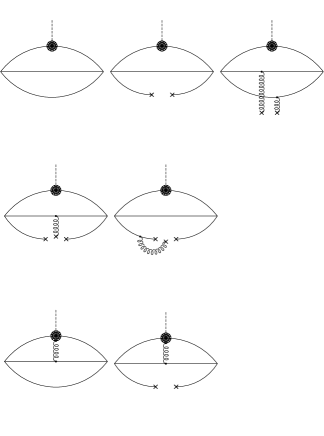
Figure 1: The OPE diagrams considered in this work. The solid lines denote quark propagators and the wavy lines denote gluon propagators. The blob in each figure denotes the matrix element, or the wave function of the external meson specified by the dashed line.

In order to construct the phenomenological side of the sum rule, we adopt the effective interaction Lagrangian with the PS type coupling. We obtain the correlation function as

PV structure $$\ \mbox{at the order}\ {\cal O}(p)\qquad-i\gamma_{5}\ooalign{\hfil/\hfil\crcr$p$}\frac{g_{mB}\lambda_{B}^{2}(t)m_{B}}{(q^{2}-m_{B}^{2})^{2}},$$ (18)

PS structure $$\ \mbox{at the order}\ {\cal O}(p^{2})\qquad i\gamma_{5}p^{2}\frac{g_{mB}\lambda_{B}^{2}(t)}{(q^{2}-m_{B}^{2})^{2}},$$ (19)

T structure $$\ \mbox{at the order}\ {\cal O}(p)\qquad\gamma_{5}\sigma_{\mu\nu}q^{\mu}p^{\nu}\frac{g_{mB}\lambda_{B}^{2}(t)}{(q^{2}-m_{B}^{2})^{2}},$$ (20)

where $\lambda_{B}(t)$ is the coupling strength of the single baryon state to the corresponding baryon interpolating field operator $J_{B}(t)$ defined by

$$\langle 0|J_{B}(0;t)|B(p)\rangle = \lambda_{B}(t)u_{B}(p),$$

and we choose the phase so that $\lambda_{B}(t)$ is real. The continuum contributions are treated approximately by assuming the QCD duality that they match the OPE at above an effective threshold, $\sqrt{s_{th}}$, which is regarded as a parameter and is determined phenomenologically.

The sum rule is obtained by matching the OPE side with the phenomenological side and by taking the Borel transformation in order to improve the predictability. The obtained sum rules are of the form,

$$g_{mB}\lambda_{B}^{2}(t)\left[\ 1+A_{mB}(t)M^{2}\ \right] = f^{\mbox{\tiny OPE}}_{\mbox{\tiny\it$m$B}}(M^{2};t)$$ (21)

where $M$ is the Borel mass and $A_{mB}$ denotes the sum of the single pole terms. Thus, the contamination from the single pole terms can be eliminated by fitting $f^{\mbox{\tiny OPE}}_{\mbox{\tiny\it$m$B}}$ by a linear function of $M^{2}$. Explicit expressions of $f^{\mbox{\tiny OPE}}_{\mbox{\tiny\it$m$B}}(M^{2};t)$ are given in Ref. DK1 .

III.2 Pertinent Dirac structure for meson-baryon coupling sum rules

We here determine the most pertinent Dirac structure for the meson-baryon coupling sum rule out of the PV, PS and T structures given above. First of all, we focus on the sensitivity to the continuum threshold, $\sqrt{s_{th}}$. We often choose $\sqrt{s_{th}}$ to be the position of the first excited state, but examine whether the result is not too sensitive to the choice. In the present case, we first set the threshold $s_{th}=2.07{\rm GeV}^{2}$ ($\sqrt{s_{th}}=1.44{\rm GeV}$), that corresponds to the Roper resonance, and $s_{th}$ is changed to $s_{th}=2.57{\rm GeV}^{2}$ ($\sqrt{s_{th}}=1.60{\rm GeV}$) to see how the sum rule is sensitive to the threshold. We find that the result from the PV sum rule changes by about 15% at the Borel mass $M^{2}=1{\rm GeV}^{2}$. We also find that the PV sum rule has a large uncertainty in the linear fitting of Eq. (21). On the other hand, the PS and T structures are insensitive to $s_{th}$. At $M^{2}=1{\rm GeV}^{2}$, the difference is only $2-3\%$ level, and the uncertainty in the linear fitting is also small. Therefore, we conclude that the sum rule from PV structure is not reliable. Kim et al., in fact, found that this sensitivity of the PV sum rule may be understood by coherent addition of the positive and negative parity excited states KLO ; Kim2 .

As the next step, we compare the PS and T sum rules, focusing on the dependence of the OPE on the baryon interpolating field (i.e. the dependence on $t$). Ideally, the physical parameter $g_{mB}$ should be independent of $t$, but in practice, the truncation of OPE brings some spurious $t$-dependence. Therefore, the above constraint tells us how the truncated OPE calculation is reliable. In Eq. (21), as the right hand side, $f^{\mbox{\tiny OPE}}_{\mbox{\tiny\it$m$B}}$, is a quadratic function of $t$, the obtained $g_{mB}\lambda_{B}^{2}(t)$ is also quadratic. In the SU(3) limit, the strength $\lambda_{B}$ should be common to all the octet baryons, and thus a “good” sum rule must give a common shape (in $t$) for the obtained $g_{mB}\lambda_{B}^{2}(t)$.

Table 1: QCD parameters in the SU(3) limit.

$\langle\bar{q}q\rangle$	$m_{0}^{2}\equiv\langle\bar{q}g_{s}\sigma\cdot Gq\rangle/\langle\bar{q}q\rangle$	$\delta^{2}$	$\langle\frac{\alpha_{s}}{\pi}G_{\mu\nu}G^{\mu\nu}\rangle$
$-(0.23~{}{\rm GeV})^{3}$	$0.8~{}{\rm GeV}^{2}$	$0.2~{}{\rm GeV}^{2}$	$(0.33~{}{\rm GeV})^{4}$

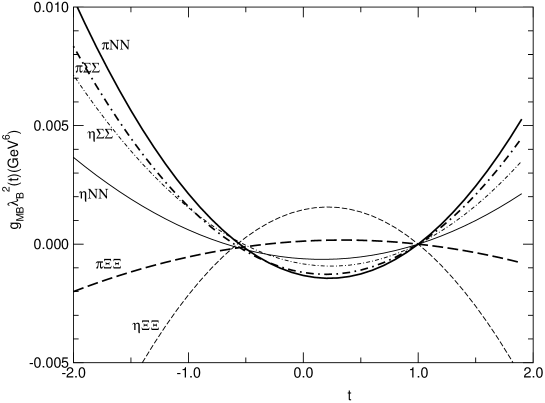
Figure 2: $g_{mB}\lambda_{B}^{2}(t)$ from the T sum rule is plotted as a function of $t$, for the $\pi NN$, $\eta NN$, $\pi\Xi\Xi$, $\eta\Xi\Xi$, $\pi\Sigma\Sigma$, and $\eta\Sigma\Sigma$ couplings. We choose the Borel window as $0.65\leq M^{2}\leq 1.24\ {\rm GeV^{2}}\$, and the continuum threshold as $s_{th}=2.07\ {\rm GeV^{2}}$.

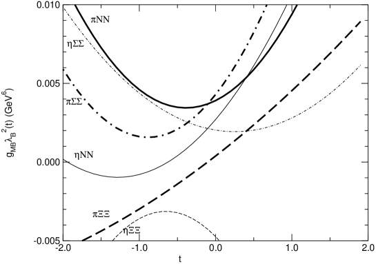
Figure 3: $g_{mB}\lambda_{B}^{2}(t)$ from the PS sum rule is plotted as a function of $t$.

Fig. 2 shows $g_{mB}\lambda_{B}^{2}(t)$ as a function of $t$ for the T sum rules, while the same for the PS sum rules is given in Fig. 3. In drawing the curves a standard set of the QCD parameters and pion matrix elements are employed, the values of which are given in Table 1. Among them, $\delta^{2}$ is defined in Eq. (62), in Appendix A, where the parametrizations of the pion matrix elements are explained.

It is interesting to see that, for the T sum rule, (1) all the curves have zeros at $t=1$ and also near $t\sim-0.6$, and (2) each curve has an extremum at around $t\sim 0.2$. One observes that the curves are well proportional to each other, indicating they are given by a single (quadratic) function of $t$, i.e., $\lambda_{B}^{2}(t)$. In contrast, the curves for the PS sum rule are random and do not show a single behavior. Therefore, we conclude that the T sum rule is more appropriate than the PS sum rule. This statement is further supported by the fact that the $t$-dependence of $\lambda_{B}^{2}(t)$ from baryon mass sum rules is consistent with that extracted from the T sum rules DK1 .

Thus we have seen that the T sum rule passes the first two criteria given in sect. III.1. In fact, the third criterion is also satisfied by the T sum rule as it does not depend on the forms of the coupling in the effective Lagrangian KLO . We conclude that the tensor (T) is the most pertinent Dirac structure.

III.3 The $F/D$ ratio of the octet meson-baryon couplings

We are now ready to construct sum rules from the $\gamma_{5}\sigma_{\mu\nu}q^{\mu}p^{\nu}$ (T) structure in the SU(3) limit and to determine the $F/D$ ratio. In particular, we investigate the $t$-dependence of the ratio using the general interpolating fields for the baryons. We consider the octet baryons $B^{a}$, and the octet mesons $m^{a}$, where $a=1\ldots 8$ denotes the flavor index for the octet representation. We note that in the SU(3) limit there is no mixing of the singlet $\eta_{1}(=m^{0})$ and the octet $\eta_{8}(=m^{8})$. The $m^{c}B^{a}B^{b}$ coupling has two independent terms, the antisymmetric (F) and symmetric (D) couplings

$${\cal L}_{F} = -F\,if_{abc}\,\bar{\psi}_{B}^{a}i\gamma^{5}\psi_{B}^{b}\phi_{m}^{c}$$

$${\cal L}_{D} = D\,d_{abc}\,\bar{\psi}_{B}^{a}i\gamma^{5}\psi_{B}^{b}\phi_{m}^{c}$$ (22)

where $f$ and $d$ are the group algebraic constants of SU(3). Then all the couplings are given by these two parameters, or equivalently in terms of

$$g_{\pi N}=(F+D)\qquad{\rm and}\qquad\alpha={F\over F+D}\ .$$ (23)

The explicit forms of the individual couplings are given by deSwart

$$g_{\eta N} = \frac{1}{\sqrt{3}}(4\alpha-1)g_{\pi N}\;;\quad g_{\pi\Xi}=(2\alpha-1)g_{\pi N}\ ,$$

$$g_{\eta\Xi} = -\frac{1}{\sqrt{3}}(1+2\alpha)g_{\pi N}\;;\quad g_{\pi\Sigma}=2\alpha\ g_{\pi N}\ ,$$

$$g_{\eta\Sigma} = g_{\pi\Lambda\Sigma}={2\over\sqrt{3}}(1-\alpha)g_{\pi N}$$ (24)

We note that our sum rules satisfy these relations at the level of the OPE expressions. This is a consequence of using the baryon interpolating fields constructed according to the SU(3) symmetry. Hence, it provides the consistency of the sum rules with the SU(3) relations for the couplings. We determine $g_{mB}$ for $m=\pi$ or $\eta$ and $B=N,\Xi$ or $\Sigma$ by linear fitting of the right hand side of Eq. (21). Taking the ratio of any two different coupling constants, we can convert it into the $F/D$ ratio according to Eq. (24).

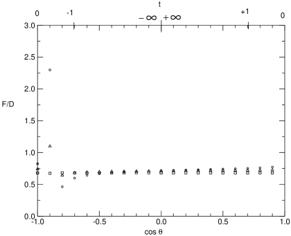
Figure 4: The $F/D$ ratio from the T sum rules is plotted as a function of $\cos\theta$, where $\theta$ is defined as $\tan\theta=t$. (See the text.) Corresponding $t$ is also shown at the top of the figure. Circles are obtained with $0.65\leq M^{2}\leq 1.24\ {\rm GeV^{2}}$ and the continuum threshold $s_{th}=2.07\ {\rm GeV^{2}}$, triangles ; $0.65\leq M^{2}\leq 1.24\ {\rm GeV^{2}}$, $s_{th}=2.57\ {\rm GeV^{2}}$, squares ; $0.90\leq M^{2}\leq 1.50\ {\rm GeV^{2}}$, $s_{th}=2.07\ {\rm GeV^{2}}$. In the realistic region $-0.75\mathrel{\mathchoice{\lower 2.58334pt\vbox{\halign{$\m@th\displaystyle\hfill#\hfil$\cr<\crcr\sim\crcr}}}{\lower 2.58334pt\vbox{\halign{$\m@th\textstyle\hfill#\hfil$\cr<\crcr\sim\crcr}}}{\lower 2.58334pt\vbox{\halign{$\m@th\scriptstyle\hfill#\hfil$\cr<\crcr\sim\crcr}}}{\lower 2.58334pt\vbox{\halign{$\m@th\scriptscriptstyle\hfill#\hfil$\cr<\crcr\sim\crcr}}}}\cos\theta\mathrel{\mathchoice{\lower 2.58334pt\vbox{\halign{$\m@th\displaystyle\hfill#\hfil$\cr<\crcr\sim\crcr}}}{\lower 2.58334pt\vbox{\halign{$\m@th\textstyle\hfill#\hfil$\cr<\crcr\sim\crcr}}}{\lower 2.58334pt\vbox{\halign{$\m@th\scriptstyle\hfill#\hfil$\cr<\crcr\sim\crcr}}}{\lower 2.58334pt\vbox{\halign{$\m@th\scriptscriptstyle\hfill#\hfil$\cr<\crcr\sim\crcr}}}}0.61$, the $F/D$ ratio is insensitive to $t$.

In Fig. 4, the $F/D$ ratio is plotted as a function of $\cos\theta$. Here, to investigate the whole range of $-\infty\leq t\leq+\infty$, we introduce a new parameter $\theta$ defined as $\tan\theta=t$. Thus, the range $0\leq t\leq+\infty$ corresponds to $0\leq\theta\leq\pi/2$ while the range $-\infty\leq t\leq 0$ spans $\pi/2\leq\theta\leq\pi$. In Fig. 4, circles are obtained from the linear fitting within the Borel window $0.65\leq M^{2}\leq 1.24\ {\rm GeV^{2}}$ with the continuum threshold $s_{th}=2.07\ {\rm GeV^{2}}$. To see the sensitivity to these parameters, we also calculate the ratio using (1) $0.65\leq M^{2}\leq 1.24\ {\rm GeV^{2}}$, $s_{th}=2.57\ {\rm GeV^{2}}$ (triangles), and (2) $0.90\leq M^{2}\leq 1.50\ {\rm GeV^{2}}$, $s_{th}=2.07\ {\rm GeV^{2}}$ (squares).

We see that the $F/D$ ratio is insensitive to the continuum threshold, as discussed before, and is also insensitive to the choice of the Borel window. The curve is flat with respect to $t$  except around the region $t\sim-0.6$ ($\cos\theta\sim-0.9$). The behavior around $t\sim-0.6$ can be understood if we remind the $t$ dependence of the coupling strengths of the baryon states to the interpolating fields, given in Fig. 2. There one sees that all the curves have a zero around $t\sim-0.6$, which indicates poor convergence of the OPE for this $t$. Thus, we conclude that the $F/D$ ratio should be obtained from the data outside $t\sim-0.6$.

Here we moderately take the appropriate region as (1) $-0.75\mathrel{\mathchoice{\lower 2.58334pt\vbox{\halign{$\m@th\displaystyle\hfill#\hfil$\cr<\crcr\sim\crcr}}}{\lower 2.58334pt\vbox{\halign{$\m@th\textstyle\hfill#\hfil$\cr<\crcr\sim\crcr}}}{\lower 2.58334pt\vbox{\halign{$\m@th\scriptstyle\hfill#\hfil$\cr<\crcr\sim\crcr}}}{\lower 2.58334pt\vbox{\halign{$\m@th\scriptscriptstyle\hfill#\hfil$\cr<\crcr\sim\crcr}}}}\cos\theta$ ($t\mathrel{\mathchoice{\lower 2.58334pt\vbox{\halign{$\m@th\displaystyle\hfill#\hfil$\cr<\crcr\sim\crcr}}}{\lower 2.58334pt\vbox{\halign{$\m@th\textstyle\hfill#\hfil$\cr<\crcr\sim\crcr}}}{\lower 2.58334pt\vbox{\halign{$\m@th\scriptstyle\hfill#\hfil$\cr<\crcr\sim\crcr}}}{\lower 2.58334pt\vbox{\halign{$\m@th\scriptscriptstyle\hfill#\hfil$\cr<\crcr\sim\crcr}}}}-0.9$)  and (2) $\cos\theta\mathrel{\mathchoice{\lower 2.58334pt\vbox{\halign{$\m@th\displaystyle\hfill#\hfil$\cr<\crcr\sim\crcr}}}{\lower 2.58334pt\vbox{\halign{$\m@th\textstyle\hfill#\hfil$\cr<\crcr\sim\crcr}}}{\lower 2.58334pt\vbox{\halign{$\m@th\scriptstyle\hfill#\hfil$\cr<\crcr\sim\crcr}}}{\lower 2.58334pt\vbox{\halign{$\m@th\scriptscriptstyle\hfill#\hfil$\cr<\crcr\sim\crcr}}}}0.61$ ($1.3\mathrel{\mathchoice{\lower 2.58334pt\vbox{\halign{$\m@th\displaystyle\hfill#\hfil$\cr<\crcr\sim\crcr}}}{\lower 2.58334pt\vbox{\halign{$\m@th\textstyle\hfill#\hfil$\cr<\crcr\sim\crcr}}}{\lower 2.58334pt\vbox{\halign{$\m@th\scriptstyle\hfill#\hfil$\cr<\crcr\sim\crcr}}}{\lower 2.58334pt\vbox{\halign{$\m@th\scriptscriptstyle\hfill#\hfil$\cr<\crcr\sim\crcr}}}}t$). The former constraint gives us the minimum value of $F/D\sim 0.55$, and the latter constraint gives us the maximum value of $F/D\sim 0.75$. Thus we obtain the final result, $F/D=0.65\pm 0.10$. We again stress that this is the determination of the $F/D$ ratio directly from (the SU(3) symmetric limit of) QCD without any assumption. Our result is very close to the value predicted in the SU(6) quark model, $F/D={2\over 3}$. This is surprising if we realize that the SU(6) symmetry, based on the nonrelativistic wave functions of three quarks in the baryons, looks fairly remote from QCD. It would be interesting to study whether this agreement has some deep reason or is just accidental. It is worth pointing out that our result is consistent with the $F/D$ ratio for the axialvector currents, $F/D\sim 0.57$, which is extracted from the semi-leptonic weak decays of the hyperons ratcliffe . It is reasonable because two $F/D$ ratios are to be related by the GT relation.

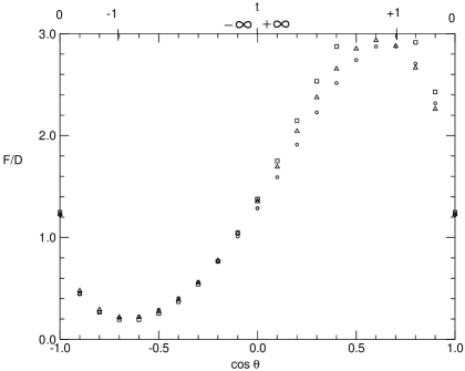
Figure 5: The $F/D$ ratio from the PS structure is plotted as a function of $\cos\theta$. See the caption of Fig. 4 for the explanation of each symbol. The $F/D$ ratio is sensitive to $t$ and no reliable prediction is obtained.

Before closing this section, let us show the result from the PS sum rule. In this case too, we can classify the OPE according to Eq. (24) and identify the terms responsible for the $F/D$ ratio. By taking similar steps as the T sum rules, we determine the $F/D$ ratio. Fig. 5 shows the $F/D$ ratio as a function of $\cos\theta$. Compared with Fig. 4, one sees that the $F/D$ ratio is highly sensitive to $t$ and the result is not reliable. Therefore, we again note that one has to carefully choose the Dirac structure in the sum rule.

The behavior of the $F/D$ ratio suggests that the PS sum rule is contaminated by continuum states, because the peak and the bottom of the curve in Fig. 5 coincide with those expected from the $F/D$ ratio of the interpolating field operators. In fact, it is shown JHO that $t=1$ ($-1$) corresponds to the pure $F$ ($D$) coupling. If the sum rule is dominated by the ground state baryon, then it should give a constant $F/D$ ratio, regardless the interpolating field. The T sum rule is such a case, while the PS sum rule seems to have significant continuum, which obeys the $F/D$ ratio of the interpolating field operator.

IV Off-Diagonal meson-baryon couplings and the SU(3) breaking effect

IV.1 Projected correlation function

The double pole structure of the correlation function is found to be crucial in extracting the coupling constant in the previous section. It requires a further analysis to generalize the sum rule to off-diagonal meson-baryon couplings, where the initial and final baryons have different masses. In this case, the ground state contribution to the correlation function is not given by a double pole, but has single pole structure. Therefore it is not possible to eliminate contamination from excited states simply by taking the double pole part of the correlation function, as was done in the diagonal couplings.

Recently, Kondo and Morimatsu KM1 proposed a novel method of extracting the coupling constant from the two-point correlation function. Although they applied their method to the $\pi NN$ coupling constant in their original work, the method is general and is in fact applicable to the off-diagonal case. Therefore we follow their prescription here, choosing the $\pi\Lambda\Sigma$ coupling as a concrete example to demonstrate the method.

We consider the vacuum-to-pion matrix element of the correlation function of the interpolating fields of $\Lambda$ and $\Sigma$:

$$\Pi(q,p)=i\int d^{4}xe^{iqx}\langle 0|{\rm T}[J_{\Sigma}(x)\bar{J}_{\Lambda}(0)]|\pi(p)\rangle\,.$$ (25)

We further define the vertex function by

$$\Gamma(q,p)=(\ooalign{\hfil/\hfil\crcr$q$}-m_{\Sigma})\Pi(q,p)(\ooalign{\hfil/\hfil\crcr$q$}^{\prime}-m_{\Lambda})$$ (30)

with $q^{\prime}\equiv q-p$. Then the $\pi\Lambda\Sigma$ coupling constant, $g\equiv g_{\pi\Lambda\Sigma}$, can be defined by the vertex function projected on to the on-mass-shell baryon states,

$$\bar{u}_{\Sigma}(\mbox{\boldmath$q$})\Gamma(q,p)u_{\Lambda}(\mbox{\boldmath$q$}^{\prime})|_{q^{2}=m_{\Sigma}^{2},(q^{\prime})^{2}=m_{\Lambda}^{2}}=i\lambda_{\Lambda}\lambda_{\Sigma}\,g\,\bar{u}_{\Sigma}(\mbox{\boldmath$q$})\gamma_{5}u_{\Lambda}(\mbox{\boldmath$q$}^{\prime}),$$ (31)

where $u(\mbox{\boldmath$q$})$ denotes the Dirac plane wave spinor (where we suppress the helicity indices for simplicity).

Advantage of defining the coupling constant in terms of the vertex function, $\Gamma$, is that it has no ambiguity originated from the choice of effective Lagrangian for the coupling. Indeed, Eqs. (30) and (31) allow us to extract the residue of the pole term on which both the baryons are on the mass shell. Such definition is known to be unique regardless of the form of the effective coupling, such as the pseudoscalar coupling or pseudovector coupling. On the other hand, in employing this new approach, we need to compute all possible terms with various Dirac structures of the correlation function, as the vertex function $\Gamma$ is a linear combination of all the terms.

It should be also noted that the kinematical point of the definition Eq. (31) is an unphysical point and that the sum rule does not give the coupling constant of that point directly. However, we will see later that the difference between the coupling constant defined by Eq. (31) and the one calculated in the sum rules is small, and therefore can be neglected.

In practical application of the sum rule to the coupling constant, we need a further elaboration so that the contamination from other poles should be small. In order to eliminate unwanted contributions from the negative energy solutions, Kondo and Morimatsu KM2 further proposed to use the projected correlation function and vertex function defined by

$$\Pi_{+}(q,p)=\bar{u}_{\Sigma}(\mbox{\boldmath$q$})\gamma_{0}\Pi(q,p)\gamma_{0}u_{\Lambda}(\mbox{\boldmath$q$}^{\prime}),$$ (32)

$$\Gamma_{+}(q,p)=\bar{u}_{\Sigma}(\mbox{\boldmath$q$})(\hbox to0.0pt{/\hss}q-m_{\Sigma})\Pi(p,q)(\hbox to0.0pt{/\hss}q^{\prime}-m_{\Lambda})u_{\Lambda}(\mbox{\boldmath$q$}^{\prime}).$$ (33)

They satisfy the relation

$$\Gamma_{+}(q,p)=(q_{0}-E_{\Sigma})(q_{0}-E_{\Lambda}-\omega_{p})\Pi_{+}(q,p),$$ (34)

where $E_{\Sigma}=\sqrt{m_{\Sigma}^{2}+\mbox{\boldmath$q$}^{2}}$, $E_{\Lambda}=\sqrt{m_{\Lambda}^{2}+\mbox{\boldmath$q$}^{{}^{\prime}2}}$ and $\omega_{p}=\sqrt{m_{\pi}^{2}+\mbox{\boldmath$p$}^{2}}$. It should be noted that $\Pi_{+}(q,p)$ has poles at $q_{0}=E_{\Sigma}$ and $q_{0}=E_{\Lambda}+\omega_{p}$ but not at $q_{0}=-E_{\Sigma}$ and $q_{0}=-(E_{\Lambda}+\omega_{p})$.

Regarding $\Pi_{+}$ and $\Gamma_{+}$ as functions of the center-of-mass energy, or $q_{0}$ in the reference frame $\mbox{\boldmath$q$}=0$, the absorptive part of the projected correlation function, ${\rm Im}\Pi_{+}$, can be written as

$${\rm Im}\Pi_{+}(q,p)= \pi\delta(q_{0}-m_{\Sigma}){{\rm Re}\Gamma_{+}(q,p)\over E_{\Lambda}+\omega_{p}-m_{\Sigma}}-\pi\delta(q_{0}-E_{\Lambda}-\omega_{p}){{\rm Re}\Gamma_{+}(q,p)\over E_{\Lambda}+\omega_{p}-m_{\Sigma}}$$ (36)

$$+{\rm Re}{1\over(q_{0}-m_{\Sigma})(q_{0}-E_{\Lambda}-\omega_{p})}{\rm Im}\Gamma_{+}(q,p).$$

Here we adopt the following notation for the dispersive (continuous) part and the absorptive (discontinuous) part, respectively:

$${\rm Re}F(q)\equiv\lim_{\eta\to 0}{1\over 2}\left[F(q)|_{q^{0}=q^{0}+i\eta}+F(q)|_{q^{0}=q^{0}-i\eta}\right],$$ (37)

$${\rm Im}F(q)\equiv\lim_{\eta\to 0}{1\over 2i}\left[F(q)|_{q^{0}=q^{0}+i\eta}-F(q)|_{q^{0}=q^{0}-i\eta}\right].$$ (38)

In Eq. (36), the first and second terms are the pole terms, which are proportional to the coupling constant, and the third term is classified as the continuum contribution. It is noted that all the terms on the right-hand side of Eq. (36) are well defined in the dispersion integral even in the chiral limit and the flavor SU(3) limit, which is another reason to employ the projected correlation function KM2 .

The dispersion relation for the projected correlation function in the variable $q_{0}$ is given by

$$\Pi_{+}(q_{0}) = -{1\over\pi}\int dq_{0}^{\prime}{{\rm Im}\Pi_{+}(q_{0}^{\prime})\over q_{0}-q_{0}^{\prime}+i\eta}.$$ (39)

By splitting the projected correlation function into the even and odd parts by

$$\Pi_{+}^{{\rm E}} = {1\over 2}[\Pi_{+}(q_{0})+\Pi_{+}(-q_{0})],$$

$$\Pi_{+}^{{\rm O}} = {1\over 2q_{0}}[\Pi_{+}(q_{0})-\Pi_{+}(-q_{0})],$$ (40)

Eq. (39) is given by

$$\Pi_{+}^{{\rm E}}(q_{0}^{2}) = -{1\over\pi}\int dq_{0}^{\prime}{q_{0}^{\prime}\over q_{0}^{2}-q_{0}^{\prime 2}}{\rm Im}\Pi_{+}(q_{0}^{\prime}),$$ (41)

$$\Pi_{+}^{{\rm O}}(q_{0}^{2}) = -{1\over\pi}\int dq_{0}^{\prime}{1\over q_{0}^{2}-q_{0}^{\prime 2}}{\rm Im}\Pi_{+}(q_{0}^{\prime}).$$ (42)

Applying the Borel transformation, $\hat{\rm L}_{M}$ defined in the Appendix B, with respect to $q_{0}^{2}$, we obtain

$$\hat{\rm L}_{M}[\Pi_{+}^{{\rm E}}] = {1\over\pi}\int dq_{0}^{\prime}{q_{0}^{\prime}\over M^{2}}\exp\left(-{{q_{0}^{\prime}}^{2}\over M^{2}}\right){\rm Im}\Pi_{+}(q_{0}^{\prime}),$$ (43)

$$\hat{\rm L}_{M}[\Pi_{+}^{{\rm O}}] = {1\over\pi}\int dq_{0}^{\prime}{1\over M^{2}}\exp\left(-{{q_{0}^{\prime}}^{2}\over M^{2}}\right){\rm Im}\Pi_{+}(q_{0}^{\prime}).$$ (44)

Evaluating the left hand side by the OPE, we obtain the Borel sum rules.

The right-hand side of Eq. (43) is expressed in terms of the observed quantities. We parameterize the absorptive part of the projected correlation function for the $\pi\Lambda\Sigma$ vertex:

$${\rm Im}\Pi_{+}(q,p) = -\bar{u}_{\Sigma}(\mbox{\boldmath$q$})i\gamma_{5}u_{\Lambda}(\mbox{\boldmath$q$}^{\prime})\pi\lambda_{\Lambda}\lambda_{\Sigma}g(q_{0},\mbox{\boldmath$p$}^{2})\left[{\delta(q_{0}-m_{\Sigma})\over q_{0}-E_{\Lambda}-\omega_{p}}+{\delta(q_{0}-E_{\Lambda}-\omega_{p})\over q_{0}-m_{\Sigma}}\right]$$ (46)

$$+\left[\theta(q_{0}-\sqrt{s_{th}})+\theta(-q_{0}-\sqrt{s_{th}})\right]{\rm Im}\Pi_{+}^{\rm OPE}(q,p),$$

where $g(q_{0},\mbox{\boldmath$p$}^{2})$ is defined by

$${\rm Re}\Gamma_{+}(q,p)=\lambda_{\Lambda}\lambda_{\Sigma}\bar{u}_{\Sigma}(\mbox{\boldmath$q$})i\gamma_{5}u_{\Lambda}(\mbox{\boldmath$q$}^{\prime})g(q_{0},\mbox{\boldmath$p$}^{2}).$$ (47)

In Eq. (46) $\sqrt{s_{th}}$ is the effective continuum threshold of the $\pi\Lambda$ or $\pi\bar{\Lambda}$ channel. We assume that the asymmetry in the continuum contribution for the positive and negative energy regions is negligible.

IV.2 $\pi\Lambda\Sigma$ coupling constant

We evaluate the $\pi\Lambda\Sigma$ coupling constant using the projected sum rule presented in sect. IV.1. Here we consider only the $t=-1$ (Ioffe) interpolating field for simplicity.

Substituting Eq. (46) into the right-hand side of Eq. (43), and taking the limit $\mbox{\boldmath$p$}^{2}\to 0$, we obtain

$$\hat{\rm L}_{M}(\Pi_{+}^{{\rm E}}) = \bar{u}(\mbox{\boldmath$q$})i\gamma_{5}u(\mbox{\boldmath$q$}^{\prime}){\lambda_{\Lambda}\lambda_{\Sigma}\over M^{2}\Delta m}\left[m_{\Sigma}g_{\Sigma}\exp\left(-{m_{\Sigma}^{2}\over M^{2}}\right)\right.$$ (48)

$$\left.\quad-(m_{\Lambda}+m_{\pi})g_{\Lambda\pi}\exp\left(-{(m_{\Lambda}+m_{\pi})^{2}\over M^{2}}\right)\right]+({\rm Cont.}),$$

for the even part and

$$\hat{\rm L}_{M}(\Pi_{+}^{{\rm O}}) = \bar{u}(\mbox{\boldmath$q$})i\gamma_{5}u(\mbox{\boldmath$q$}^{\prime}){\lambda_{\Lambda}\lambda_{\Sigma}\over M^{2}\Delta m}\left[g_{\Sigma}\exp\left(-{m_{\Sigma}^{2}\over M^{2}}\right)\right.$$ (49)

$$\left.\quad-g_{\Lambda\pi}\exp\left(-{(m_{\Lambda}+m_{\pi})^{2}\over M^{2}}\right)\right]+({\rm Cont.}),$$

for the odd part, where we define $\Delta m\equiv m_{\Lambda}+m_{\pi}-m_{\Sigma}$, $g_{\Sigma}\equiv g(m_{\Sigma},\,\mbox{\boldmath$p$}^{2}=0)$ and $g_{\Lambda\pi}\equiv g(m_{\Lambda}+m_{\pi},\,\mbox{\boldmath$p$}^{2}=0)$. $({\rm Cont.})$ denotes the continuum contribution coming from the last term of Eq. (46), in which we employ the QCD duality assumption and replace it by the corresponding OPE of the correlation function at $|q_{0}|>\sqrt{s_{th}}$.

In Eqs. (48) and (49), one sees that the poles bring the coupling constant at two different kinematical points, $g_{\Sigma}\equiv g(m_{\Sigma},0)$ and $g_{\Lambda\pi}\equiv g(m_{\Lambda}+m_{\pi}=m_{\Sigma}+\Delta m,0)$, while the one defined in Eq. (31) is at the kinematical point, $q^{2}=m_{\Sigma}^{2}$, $q^{{}^{\prime}2}=m_{\Lambda}^{2}$, i.e.,

$$g=g\left(q_{0}=m_{\Sigma},{\mbox{\boldmath$p$}}^{2}=-m_{\pi}^{2}+{(m_{\Sigma}^{2}+m_{\pi}^{2}-m_{\Lambda}^{2})^{2}\over 4m_{\Sigma}^{2}}\right).$$ (50)

Therefore in principle we need an interpolation. However, we expect that the differences are small because $m_{\pi}$ and $\Delta m$ are both small compared to the baryon masses. Thus we will regard $g_{\Sigma}$ in the sum rule as the coupling constant.

The sum rules are obtained by equating these Borel-transformed correlation functions with the corresponding OPE terms. The OPE’s of $\Pi_{+}^{{\rm E}}$ and $\Pi_{+}^{{\rm O}}$ are rather lengthy and therefore we give the explicit forms in Appendix B. In order to evaluate $g_{\Sigma}$, we operate

$$\hat{\rm P}_{\Sigma}\equiv(m_{\Lambda}+m_{\pi})^{2}-M^{2}{\partial\over\partial M^{2}}M^{2}$$

on the both sides of the sum rule and eliminate the $g_{\Lambda\pi}$ terms. Then we obtain

$$g_{\Sigma}\,{m_{\Sigma}(m_{\Sigma}+m_{\Lambda}+m_{\pi})\over M^{2}}\exp\left(-{m_{\Sigma}^{2}\over M^{2}}\right) = \hat{\rm P}_{\Sigma}\left[{\bar{\Pi}_{+}^{{\rm E}}(M)\over\lambda_{\Lambda}\lambda_{\Sigma}}\right],$$ (51)

$$g_{\Sigma}\,{m_{\Sigma}+m_{\Lambda}+m_{\pi}\over M^{2}}\exp\left(-{m_{\Sigma}^{2}\over M^{2}}\right) = \hat{\rm P}_{\Sigma}\left[{\bar{\Pi}_{+}^{{\rm O}}(M)\over\lambda_{\Lambda}\lambda_{\Sigma}}\right]$$ (52)

with $\bar{\Pi}_{+}^{{\rm E}/{\rm O}}(M)$ given in Appendix B. The unknown constants, $\lambda_{\Lambda}$ and $\lambda_{\Sigma}$, are calculated from the vacuum-to-vacuum sum rule (mass sum rule) with the same interpolating fields and the Borel mass, whose explicit forms are also given in Appendix B.

In numerical analyses, the threshold parameters, $\sqrt{s_{th}}$ for $\Pi_{+}$, and $\sqrt{s_{0}}$ for the $\Lambda$ and $\Sigma$ mass sum rules, given in Eqs. (92) and (95), are chosen to be equal, because the continuum mainly comes from the $S=-1$ excited baryons and therefore is expected to be common to $\Pi_{+}$ and the mass sum rules.

Two sum rules, Eqs. (51) and (52), should in principle give the same result. However, we have seen in sect. III that the results depend on the choice of the Dirac structure and that the tensor (T) sum rule is most reliable because it contains less contribution from the continuum and has weaker dependence on the choice of the interpolating field. In the present off-diagonal case, we employ the same criteria. In fact, from the structure of the $\bar{\Pi}_{+}^{{\rm E}/{\rm O}}$, we find that $\Pi_{+}^{{\rm O}}$ is superior to $\Pi_{+}^{{\rm E}}$ because $\Pi_{+}^{{\rm O}}$ contains mainly the T structure and therefore is less dependent on the continuum. Actually, it is easy to check that $\Pi_{+}^{{\rm O}}$ reduces to the OPE of the T structure in the chiral limit. In order to quantify this statement, we check how large the continuum contribution is in each sum rule. A numerical analysis tells us that (in the SU(3) limit) about 40% of the continuum contribution comes from the region above the threshold for the $\Pi_{+}^{{\rm E}}$ sum rule, Eq. (51), while it is less than 16% for the $\Pi_{+}^{{\rm O}}$ sum rule, Eq. (52). Therefore we conclude that $\Pi_{+}^{{\rm O}}$ sum rule is more reliable.

Another advantage of the $\Pi_{+}^{{\rm O}}$ sum rule is that the main term in OPE is proportional to the $\langle\bar{q}q\rangle$ condensate, which is divided out by the main term of the baryon mass sum rule, This elimination of the $\langle\bar{q}q\rangle$ condensate reduces ambiguity in the numerical results. Thus we employ the $\Pi_{+}^{{\rm O}}$ sum rule in the following analysis.

IV.3 Results

We evaluate the $\pi\Lambda\Sigma$ coupling constant both in the SU(3) limit and in the realistic broken SU(3) case. In getting the final values, we choose the parameter according to Table 2, except that in the SU(3) limit, we make $m_{s}=m_{u}\sim 0$ and $\langle\bar{s}s\rangle=\langle\bar{u}u\rangle$. When we take the SU(3) limit, we use the nucleon mass for both the $\Lambda$ and $\Sigma$ masses, while in the broken SU(3) calculation, the observed masses of the baryons are used. To get the final results, we have to choose the threshold parameter and the Borel mass window. In the SU(3) limit, the choice given in sect. III.3 is taken, that is, $2.07\leq s_{th}=s_{0}\leq 2.57\ {\rm GeV}^{2}$ and $0.65\leq M^{2}\leq 1.24\ {\rm GeV^{2}}$. In the broken SU(3) case, we set the threshold to above the first excited state of $\Sigma$ resonance, $2.76\leq s_{th}=s_{0}\leq 3.27\ {\rm GeV}^{2}$ ($\sqrt{s_{th}}=\sqrt{s_{0}}\sim 1.66-1.81$ GeV) and consider the Borel window, $1.00\leq M^{2}\leq 1.69\ {\rm GeV^{2}}$.

Table 2: QCD parameters. We always assume that $\langle\bar{d}d\rangle=\langle\bar{u}u\rangle$, and employ the same $m_{0}^{2}\equiv{\langle\bar{q}g_{s}\sigma\cdot Gq\rangle\over\langle\bar{q}q\rangle}$ for the $u$, $d$ and $s$ quarks. The OPE terms which are proportional to $m_{u}$ or $m_{d}$ are neglected, that is equivalent to the choice $m_{u}=m_{d}=0$.

$\langle\bar{u}u\rangle$	$\langle\bar{s}s\rangle/\langle\bar{u}u\rangle$	$m_{s}$	$m_{0}^{2}$	$\delta^{2}$	$\langle\frac{\alpha_{s}}{\pi}G_{\mu\nu}G^{\mu\nu}\rangle$
$-(0.23~{}{\rm GeV})^{3}$	0.8	$0.12{\rm GeV}$	$0.8~{}{\rm GeV}^{2}$	$0.2~{}{\rm GeV}^{2}$	$(0.33~{}{\rm GeV})^{4}$

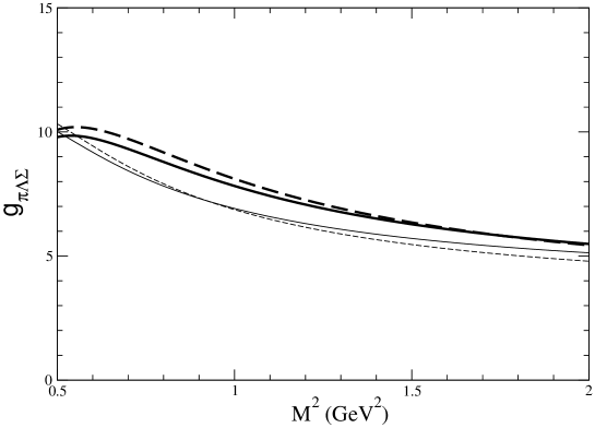
Figure 6: $g_{\pi\Lambda\Sigma}$ from the $\Pi_{+}^{{\rm O}}$ sum rule plotted against the squared Borel mass $M^{2}$. Thin solid (dashed) line denotes $g_{\pi\Lambda\Sigma}$ in the SU(3) limit using the continuum threshold $s_{th}=s_{0}=2.07$ (2.57) ${\rm GeV}^{2}$. Thick solid (dashed) line denotes $g_{\pi\Lambda\Sigma}$ including the SU(3) breaking effects using $s_{th}=s_{0}=2.76$ (3.26) ${\rm GeV}^{2}$.

Fig. 6 gives the resulting Borel curves for the SU(3) limit and for the broken SU(3) case. Comparing the solid lines with the corresponding dashed lines, we confirm that the results are not sensitive to the choice of the continuum threshold.

The final results can be read off from the Borel curves by averaging over the values inside a Borel window. One sees that the curves for the SU(3) limit are slightly lower than those in the broken SU(3) case. We, however, have to shift the Borel window as given above so as to take account of the larger $\Lambda$ and $\Sigma$ masses. We use the Borel window $0.65\leq M^{2}\leq 1.24{\rm GeV}^{2}$ in the SU(3) limit and $1.00\leq M^{2}\leq 1.69{\rm GeV}^{2}$ in the broken SU(3) case. In the end, the obtained values of the coupling constants have little difference. Then we obtain

$$g_{\pi\Lambda\Sigma}(\hbox{SU(3) limit})=7.5\pm 1.3,$$

$$g_{\pi\Lambda\Sigma}(\hbox{broken SU(3)})=6.9\pm 1.0.$$

As these numbers are consistent with each other, we conclude that the effect of the SU(3) breaking is weak in the $\pi\Lambda\Sigma$ coupling.

In the SU(3) limit the coupling constant, $g_{\pi\Lambda\Sigma}$, must be related to the $g_{\pi N}$ through the relation given in terms of the $F/D$ ratio, Eq. (24),

$$g_{\pi\Lambda\Sigma}={2\over\sqrt{3}}(1-\alpha)g_{\pi N}.$$

In order to see this relation, we apply the sum rule derived from the projected correlation function to $g_{\pi N}$. Using the same parameters, the continuum threshold and the Borel mass window, we obtain $g_{\pi N}\sim 9.6\pm 1.6$, which corresponds to $F/D=0.47$ ($\alpha=0.32$). This value is smaller than $F/D=0.65\pm 0.10$ determined from the T sum rule in sect. III.3. This discrepancy is attributed mainly to the ambiguity brought by the mass sum rule, by which the correlation function is divided in order to eliminate the factor $\lambda_{\Lambda}\lambda_{\Sigma}$ or $\lambda_{N}^{2}$. Generally the mass sum rule has moderate Borel mass dependence and therefore causes some ambiguity. Note that the $F/D$ ratio is obtained without using the mass sum rule in sect. III.3. A further discrepancy may come from the difference in the method of extracting the coupling constant. Sum rules constructed by the derivative with respect to the Borel mass are in general less trustable than the global Borel mass fit. Another source of discrepancy is the difference in the choice of the interpolating field. As was pointed out in sect. III.3, the $F/D$ ratio from the interpolating field à la Ioffe ($t=-1$) tends to be underestimated. We indeed see in Fig. 4 that the $F/D$ ratio at $t=-1$ is rather below the central value. We also suspect that the $F/D$ ratio from the projected sum rule contains some spurious $t$-dependence because we do not take the chiral limit and then the OPE has contributions from the PS and PV structure. Thus we conclude that the $F/D$ ratio obtained in the T sum rule is more reliable than that given here.

The value of $g_{\pi N}$ is consistent with the previous sum rule calculations, but it is smaller than the value determined from the strength of the one-pion exchange potential. This discrepancy is still an open problem.

Earlier, an attempt was made to compute the $g_{\pi\Lambda\Sigma}$ coupling constant using the three-point correlation function by Choe Choe , giving $g_{\pi\Lambda\Sigma}\sim 10.79$, a larger number than our result. It should, however, be noted that the $p^{2}\to 0$ limit is taken to evaluate the coupling constant, which, as we stressed in sect. II, is not allowed in computing the OPE.

Recently, Lutz and Kolomeitsev Lutz performed an extensive analysis of experimental data using relativistic chiral SU(3) formulation. They have obtained the coupling constants from fitting to the scatterings data and obtain, among others, $g_{\pi\Lambda\Sigma}\sim 10.4$, which is somewhat larger than our prediction. On the other hand, a recent coupled-channel analysis of the $\bar{K}N$ scattering has predicted much smaller value Keil . The obtained value, $g_{\pi\Lambda\Sigma}/g_{\pi N}\sim 0.4$, suggests a large SU(3) violation, while our result is consistent with SU(3) symmetry with $\alpha\sim 0.4$.

V Conclusion

As the fundamental theory of the strong interaction, QCD is to be applied directly to the hadronic interactions. We have presented a part of such attempts that the meson-baryon coupling constants are calculated in the QCD sum rule approach. It is shown that the coupling constants are expressed in terms of the nonperturbative QCD parameters, such as the quark condensates, gluon condensates, as well as the pion (light-cone) wave functions.

We have addressed several technical issues in this report. (1) It is advantageous to take the two-point correlation function of baryons to derive sum rules for the coupling constants. The correlation function is evaluated for the initial meson state and the final vacuum so that the coupling vertex appears in the middle. (2) We have considered the analytic structures of the correlation function and have pointed out that the double pole term, one pole from the initial baryon and the other from the final baryon, is carefully taken out to evaluate the coupling constant. (3) In the case of the baryon-diagonal couplings, the double pole is easily extracted by the Borel transform, and we have found that the most appropriate Dirac structure in the two point function is the tensor type, proportional to $\gamma^{5}\sigma_{\mu\nu}q^{\mu}p^{\nu}$. Especially, this choice avoids spurious dependence on the choice of the interpolating field operator for the octet baryons. (4) In order to derive workable sum rule for the baryon-off-diagonal couplings, we have found that the projected correlation function is most useful. Among the two sum rules, even (E) and odd (O), we have found that the odd one gives the most reliable result.

We have emphasized that the SU(3) symmetry must be recovered if we turn off the quark mass differences. Then the coupling constants of the SU(3) octet mesons and octet baryons can be expressed in terms of two constants, overall constant, represented by $g_{\pi N}$ for instance, and the $F/D$ ratio. Because the $F/D$ ratio is a completely free parameter not determined by the SU(3) symmetry, it is important and interesting to determine this ratio directly from QCD. We have found that the sum rule in the SU(3) limit is fully consistent with SU(3) and gives $F/D=0.65\pm 0.10$, which almost coincides with the value derived from the quark model, or the SU(6) spin-flavor symmetry, $F/D={2\over 3}$, or $\alpha\equiv{F\over F+D}=0.4$. This is also consistent with the $F/D$ ratio of the axialvector coupling constants obtained from the beta decay rates of the hyperons.

We have calculated the $\pi\Lambda\Sigma$ coupling constant as an example of the baryon-off-diagonal coupling. We have found that the effect of the SU(3) breaking is small by comparing the results in the SU(3) limit, $g_{\pi\Lambda\Sigma}=7.5\pm 1.3$, and in the broken SU(3) case, $g_{\pi\Lambda\Sigma}=6.9\pm 1.0$. In fact, even at the level of the OPE, it can be seen that effects of the SU(3) breaking are weak as far as the pion-baryon couplings are concerned. The SU(3) breaking is taken into account in the QCD sum rule as the quark mass term, $m_{s}\neq m_{u}$ and indirectly in terms of the difference in the quark condensates, $\langle\bar{s}s\rangle\neq\langle\bar{u}u\rangle$ and $\langle\bar{s}g_{s}\sigma\cdot Gs\rangle\neq\langle\bar{u}g_{s}\sigma\cdot Gu\rangle$. However, both of these contributions do not appear in the leading terms of OPE for the pion-baryon couplings. Thus we see that not only the $\pi\Lambda\Sigma$ coupling, but also the other $\pi$-baryon couplings, like $\pi\Sigma\Sigma$, and $\pi\Xi\Xi$, may not deviate much from the SU(3) values.

It is, however, not the case when we consider the couplings of the $\eta$, and maybe $K$, mesons. The sum rule involves the meson mass, $m_{\eta,K}$ and the decay constants, $f_{\eta,K}$, in the leading terms. Therefore the SU(3) breaking of order a few tens of per cent can easily predicted in the QCD sum rule KD1 .

In future analyses, it is desirable to calculate the $KB_{1}B_{2}$ couplings, such as $KN\Lambda$ and $KN\Sigma$, which are phenomenologically very important, for instance, in the hypernuclear physics.

Appendix A

We calculate the Wilson coefficients of the short-distance expansion in two steps: we perform the light-cone expansion of the correlation function first and the short-distance expansion of the light-cone operators second. The reason for doing this is to use the parametrization of the vacuum-to-pion matrix elements of the light-cone operators given in Ref. Belyaev ,

$$\langle 0|\bar{u}i\gamma_{5}u|\pi^{0}(p)\rangle = -\frac{\langle\bar{u}u\rangle}{f_{\pi}}+i(p\cdot x)\frac{\langle\bar{u}u\rangle}{2f_{\pi}}+(p\cdot x)^{2}\frac{\langle\bar{u}u\rangle}{2f_{\pi}}(\frac{1}{3}+\frac{1}{30}B_{2})$$ (53)

$$+{\cal O}((p\cdot x)^{3})$$

$$\langle 0|\bar{u}\gamma_{\mu}\gamma_{5}u|\pi^{0}(p)\rangle = if_{\pi}p_{\mu}+\frac{1}{2}f_{\pi}(p\cdot x)p_{\mu}$$ (54)

$$-\frac{1}{18}if_{\pi}\delta^{2}(p\cdot x)x_{\mu}+\frac{5}{36}if_{\pi}\delta^{2}x^{2}p_{\mu}$$

$$+\frac{5}{72}f_{\pi}\delta^{2}(p\cdot x)x^{2}p_{\mu}-\frac{1}{36}f_{\pi}\delta^{2}(p\cdot x)^{2}x_{\mu}$$

$$+{\cal O}(p^{3}x^{3})+{\cal O}((p)^{0}x^{4})$$

$$\langle 0|\bar{u}\gamma_{5}\sigma_{\mu\nu}u|\pi^{0}(p)\rangle = -i(p_{\mu}x_{\nu}-p_{\nu}x_{\mu})\frac{\langle\bar{u}u\rangle}{6f_{\pi}}\left(1-\frac{1}{2}i(p\cdot x)\right)+{\cal O}((p\cdot x)^{3})$$ (55)

$$\langle 0|u^{a}(x)g_{s}G^{A}_{\mu\nu}(vx)\bar{u}^{b}(0)|\pi^{0}(p)\rangle$$ (61)

$$= +i\frac{f_{3\pi}}{16\sqrt{2}}t^{A}_{ab}\left[\gamma_{5}\sigma_{\lambda\mu}p^{\lambda}p_{\nu}-\gamma_{5}\sigma_{\lambda\nu}p^{\lambda}p_{\mu}\right]$$

$$+\frac{if_{\pi}\delta^{2}}{252\cdot 16}t^{A}_{ab}\Big{[}\ +(7+6\epsilon)\ (\gamma_{5}\gamma_{\mu}p_{\nu}-\gamma_{5}\gamma_{\nu}p_{\mu})\ (p\cdot x)$$

$$\qquad\qquad\qquad\quad+(7+18\epsilon)\ \gamma_{5}\ooalign{\hfil/\hfil\crcr$p$}\ (p_{\mu}x_{\nu}-p_{\nu}x_{\mu})\ \Big{]}$$

$$-\frac{1}{16}\ t^{A}_{ab}\ \epsilon_{\mu\nu}^{\ \ \ \alpha\beta}$$

$$\qquad\times\Big{[}+if_{\pi}\delta^{2}\ \gamma_{\alpha}p_{\beta}\ \left\{\frac{1}{3}-\frac{i}{84}(p\cdot x)(7+6\epsilon-2v(-7+6\epsilon))\right\}$$

$$\qquad\qquad+f_{\pi}\delta^{2}\ \ooalign{\hfil/\hfil\crcr$p$}\ p_{\alpha}x_{\beta}\ \left\{\frac{1}{252}(-7+6\epsilon)+\frac{1}{126}v(7-6\epsilon)\right\}\ \Big{]}$$

Here $t^{A}\equiv{\lambda^{A}\over 2}$ is the color SU(3) generator, $g_{s}$ is the renormalized coupling constant of the QCD and $G_{\rho\sigma}^{A}$ is the gluon field tensor. We also define $G_{\alpha\beta}\equiv\sum_{A}G_{\alpha\beta}^{A}t^{A}$ and $\tilde{G}_{\alpha\beta}\equiv{1\over 2}\epsilon_{\alpha\beta\mu\nu}G^{\mu\nu}$ with $\epsilon_{0123}=-\epsilon^{0123}=1$.

Several parameters arise in the matrix elements: $f_{\pi}$ ($=93$ MeV) is the pion decay constant, $f_{3\pi}$ ($=0.0035({\rm GeV})^{2}$) and $B_{2}\equiv-{30\over\sqrt{2}}{f_{3\pi}f_{\pi}\over\langle\bar{u}u\rangle}$ ($=0.57$) are the parameters coming from the twist-3 pion wave function, and $\epsilon$ ( $=0.5$) is from the twist-4 pion wave functions Belyaev . We choose 1 GeV for the renormalization scale.

The $\delta^{2}$ is another parameter from the twist-4 pion wave function defined, according to Novikov et al. Novikov , by

$$\langle 0|\bar{d}g_{s}\tilde{G}_{\mu\nu}\gamma^{\nu}u|\pi^{+}(p)\rangle=\sqrt{2}if_{\pi}\delta^{2}p_{\mu}\,.$$ (62)

In previous calculations, however, there was some confusion on the sign of this constant. Therefore, we here estimate $\delta^{2}$ in our notation according to Ref. CZ .

Let us consider the correlation function

$$T_{\mu}=i\int dxe^{iqx}\langle{0|T[\bar{d}(x)\gamma_{\mu}\gamma_{5}g_{s}\sigma^{\alpha\beta}G_{\alpha\beta}u(x)\bar{u}(0)\gamma_{5}d(0)]|0}\rangle.$$ (63)

Using the formula $\langle{0|:q^{a}\bar{q}^{b}g_{s}G_{\alpha\beta}^{h}:|0}\rangle t^{h}_{ba}=-{1\over 48}\langle{0|\bar{q}g_{s}\sigma^{\mu\nu}G_{\mu\nu}q|0}\rangle\sigma_{\alpha\beta}$, we calculate the OPE of the correlation function, which gives to the lowest dimension

$$T_{\mu} = \langle{\bar{u}g_{s}\sigma^{\alpha\beta}G_{\alpha\beta}u}\rangle\,{q_{\mu}\over q^{2}}.$$ (64)

The spectral function of the correlation function is given by

$${1\over\pi}{\rm Im}T_{\mu} = (2\pi)^{3}\sum_{n}\left\{\delta^{4}(p-q)\langle{0|\bar{d}\gamma_{\mu}\gamma_{5}{g_{s}\sigma_{\alpha\beta}G^{\alpha\beta}}u|n\rangle\langle n|\bar{u}\gamma_{5}d|0}\rangle\right.$$ (66)

$$+\delta^{4}(p+q)\left.\langle{0|\bar{u}\gamma_{5}d|n\rangle\langle n|\bar{d}\gamma_{\mu}\gamma_{5}{g_{s}\sigma_{\alpha\beta}G^{\alpha\beta}}u|0}\rangle\right\}$$

$$= (2\pi)^{3}\int{d^{3}p\over(2\pi)^{3}2\omega_{p}}\left\{\delta^{4}(p-q)\langle{0|\bar{d}\gamma_{\mu}\gamma_{5}{g_{s}\sigma_{\alpha\beta}G^{\alpha\beta}}u|\pi^{+}(p)\rangle\langle\pi^{+}(p)|\bar{u}\gamma_{5}d|0}\rangle\right.$$ (68)

$$+\left.\delta^{4}(p+q)\langle{0|\bar{u}\gamma_{5}d|\pi^{-}(p)\rangle\langle\pi^{-}(p)|\bar{d}\gamma_{\mu}\gamma_{5}{g_{s}\sigma_{\alpha\beta}G^{\alpha\beta}}u|0}\rangle\right\}+\hbox{(non-pion pole terms)}$$

$$= \delta(q^{2}-m_{\pi}^{2})q_{\mu}{2f_{\pi}^{2}m_{\pi}^{2}\over m_{u}+m_{d}}A+\hbox{(non-pion pole terms)}.$$ (69)

The constant $A$ is defined by

$$\langle{0|\bar{d}\gamma_{\mu}\gamma_{5}g_{s}\sigma^{\alpha\beta}G_{\alpha\beta}u|\pi^{+}(p)}\rangle \equiv i\sqrt{2}f_{\pi}p_{\mu}A,$$ (70)

$$\langle{\pi^{-}(p)|\bar{d}\gamma_{\mu}\gamma_{5}{g_{s}\sigma_{\alpha\beta}G^{\alpha\beta}}u|0}\rangle \simeq -i\sqrt{2}f_{\pi}p_{\mu}A,$$ (71)

where we use the fact that $\langle{\pi^{-}(p)|\bar{d}ig_{s}{G_{\mu}}^{\beta}\gamma_{\beta}\gamma_{5}u|0}\rangle$ is of higher order in the chiral expansion Novikov . The phases of the pion states are taken as

$$\langle{0|\bar{d}\gamma_{\mu}\gamma_{5}u|\pi^{+}(p)}\rangle = i\sqrt{2}f_{\pi}p_{\mu}$$ (72)

$$\langle{0|\bar{u}\gamma_{\mu}\gamma_{5}d|\pi^{-}(p)}\rangle = i\sqrt{2}f_{\pi}p_{\mu}.$$ (73)

Substituting Eq. (64) and Eq. (66) for the left-hand and the right-hand sides of the dispersion relation as follows

$$T(q^{2})=-{1\over\pi}\int_{0}^{\infty}ds{{\rm Im}T(s)\over q^{2}-s},$$ (74)

respectively, at $Q^{2}=-q^{2}\rightarrow\infty$ we obtain

$$\langle{\bar{u}g_{s}\sigma^{\alpha\beta}G_{\alpha\beta}u}\rangle\,{q_{\mu}\over Q^{2}}=-{2f_{\pi}^{2}m_{\pi}^{2}\over m_{u}+m_{d}}\,{q_{\mu}A\over Q^{2}+m_{\pi}^{2}}.$$ (75)

Taking the chiral limit and using the relation $f_{\pi}^{2}m_{\pi}^{2}=-(m_{u}+m_{d})\langle\bar{u}u\rangle$, we find

$$A={\langle{\bar{u}g_{s}\sigma^{\alpha\beta}G_{\alpha\beta}u}\rangle\over 2\langle\bar{u}u\rangle}={m_{0}^{2}\over 2}.$$ (76)

Using the identity, $\gamma_{\mu}\sigma_{\alpha\beta}=i(g_{\mu\alpha}\gamma_{\beta}-g_{\mu\beta}\gamma_{\alpha})+\epsilon_{\mu\alpha\beta\nu}\gamma^{\nu}\gamma_{5}$, one can rewrite the matrix element (70) as

$$\langle{0|\bar{d}g_{s}\gamma_{\mu}\gamma_{5}\sigma_{\alpha\beta}G^{\alpha\beta}u|\pi^{+}(p)}\rangle = 2\langle{0|\bar{d}ig_{s}{G_{\mu}}^{\beta}\gamma_{\beta}\gamma_{5}u|\pi^{+}(p)}\rangle+2\langle{0|\bar{d}g_{s}\tilde{G}_{\mu\nu}\gamma^{\nu}u|\pi^{+}(p)}\rangle.$$ (77)

The first term in this expression is of higher order in the chiral expansion Novikov . ¿From Eqs. (62) and (70), we obtain

$$\delta^{2}={m_{0}^{2}\over 4}\sim 0.2\;{\rm GeV}^{2}.$$ (78)

The sign of $\delta^{2}$ is therefore determined by that of $m_{0}^{2}$, which has been relatively well studied as a (higher dimensional) chiral order parameter. In the analysis in ref. BK1 , the $\delta^{2}$ with the opposite sign was used, which was transferred to some of the subsequent studies KD1 ; DK1 ; KM2 ; DK2 . The wrong sign of $\delta^{2}$ happens to give a larger value of the $\pi NN$ coupling constant, which tends to agree with experimental data. In fact, if we use the correct $\delta^{2}$, then the coupling constants are reduced by about 30 % or so and the agreement with data is somewhat spoiled.

Appendix B

The operator product expansion (OPE) sides of the $\Pi_{+}^{{\rm E}}$ and $\Pi_{+}^{{\rm O}}$ defined in Eq. (40) for the $\pi\Lambda\Sigma$ coupling constant are explicitly given in this Appendix.

We define the correlation functions by

$$\Pi(q,p) \equiv i\int d^{4}xe^{iqx}\langle 0|{\rm T}[J_{\Sigma^{0}}(x)\ \bar{J}_{\Lambda}(0)]|\pi^{0}(p)\rangle,$$ (79)

$$\Pi_{+}(q,p) \equiv \bar{u}_{\Sigma}(\mbox{\boldmath$q$})\gamma_{0}\Pi\gamma_{0}u_{\Lambda}(\mbox{\boldmath$q$}-\mbox{\boldmath$p$}),$$ (80)

$$\Pi_{+}^{{\rm E}}(q_{0}) \equiv \frac{1}{2}\left[\Pi_{+}(q_{0})+\Pi_{+}(-q_{0})\right],$$ (81)

$$\Pi_{+}^{{\rm O}}(q_{0}) \equiv \frac{1}{2q_{0}}\left[\Pi_{+}(q_{0})-\Pi_{+}(-q_{0})\right],$$ (82)

where the baryon interpolating fields are chosen according to Ioffe Ioffe (that is, $t=-1$) as

$$J_{\Lambda}(x) = \sqrt{\frac{2}{3}}\epsilon_{abc}\left([u_{a}^{T}C\gamma_{\mu}s_{b}]\gamma_{5}\gamma^{\mu}d_{c}-[d_{a}^{T}C\gamma_{\mu}s_{b}]\gamma_{5}\gamma^{\mu}u_{c}\right),$$ (83)

$$J_{\Sigma^{0}}(x) = \sqrt{2}\epsilon_{abc}\left([u_{a}^{T}C\gamma_{\mu}s_{b}]\gamma_{5}\gamma^{\mu}d_{c}+[d_{a}^{T}C\gamma_{\mu}s_{b}]\gamma_{5}\gamma^{\mu}u_{c}\right).$$ (84)

We subtract the continuum contribution from the $\Pi_{+}^{{\rm E}/{\rm O}}$, assuming the threshold parameter, $\sqrt{s_{th}}$, and then apply the Borel transform

$$\hat{\rm L}_{M}\equiv\lim_{{n\rightarrow\infty\atop-q_{0}^{2}\rightarrow\infty}\atop-q_{0}^{2}/n=M^{2}}{(q_{0}^{2})^{n}\over(n-1)!}\left(-{d\over dq_{0}^{2}}\right)^{n},$$ (85)

where $M$ is the Borel mass.

Finally, we obtain

$$\bar{\Pi}^{\rm E}_{+}(M^{2})\equiv$$ (86)

$$\frac{4}{\sqrt{3}}\Biggl{\{}M^{2}C_{2}(\sqrt{s_{th}})\biggl{[}\frac{1}{8\pi^{2}}\frac{\langle\bar{q}q\rangle}{f_{\pi}}+\frac{7}{48\pi^{2}}f_{\pi}(E_{\Lambda}+m_{\Lambda}-\omega_{p})-\frac{1}{24\pi^{2}}f_{\pi}\omega_{p}\biggr{]}$$

$$\quad+C_{1}(\sqrt{s_{th}})\biggl{[}\ \left(-\frac{1}{12\pi^{2}}f_{\pi}\delta^{2}+\frac{1}{16\pi^{2}}\frac{\langle\bar{q}q\rangle}{f_{\pi}}(m_{q}-2m_{s})\right)(E_{\Lambda}+m_{\Lambda}-\omega_{p})\biggr{]}$$

$$\quad+\frac{1}{M^{2}}\biggl{[}\ -\frac{1}{48}\langle\frac{\alpha_{s}}{\pi}G_{\mu\nu}G^{\mu\nu}\rangle\frac{\langle\bar{q}q\rangle}{f_{\pi}}+\frac{1}{6}\frac{\langle\bar{q}q\rangle}{f_{\pi}}(m_{q}\langle\bar{q}q\rangle+m_{s}\langle\bar{s}s\rangle)-\frac{2}{3}\frac{\langle\bar{q}q\rangle}{f_{\pi}}(m_{q}\langle\bar{s}s\rangle+m_{s}\langle\bar{q}q\rangle)$$

$$\qquad\qquad+\left(-\frac{1}{6}\frac{\langle\bar{q}q\rangle}{f_{\pi}}\{\langle\bar{q}q\rangle-\frac{4}{3}\langle\bar{s}s\rangle\}+\frac{5}{288}\langle\frac{\alpha_{s}}{\pi}G_{\mu\nu}G^{\mu\nu}\rangle f_{\pi}\right.$$

$$\quad\quad\quad\quad\quad\left.+\frac{1}{4}f_{\pi}(m_{q}\langle\bar{q}q\rangle+m_{s}\langle\bar{s}s\rangle)-\frac{1}{3}f_{\pi}(m_{q}\langle\bar{s}s\rangle+m_{s}\langle\bar{q}q\rangle)\right)(E_{\Lambda}+m_{\Lambda}-\omega_{p})$$

$$\qquad\qquad+\left(-\frac{1}{3}\frac{\langle\bar{q}q\rangle}{f_{\pi}}\{\langle\bar{q}q\rangle-\frac{2}{3}\langle\bar{s}s\rangle\}+\frac{1}{144}\langle\frac{\alpha_{s}}{\pi}G_{\mu\nu}G^{\mu\nu}\rangle f_{\pi}\right)\omega_{p}-\frac{1}{3}f_{\pi}\langle\bar{q}q\rangle\omega_{p}(E_{\Lambda}+m_{\Lambda})\biggr{]}$$

$$\quad+\frac{1}{M^{4}}\biggl{[}\ -\frac{1}{12}\frac{\langle\bar{q}q\rangle}{f_{\pi}}(m_{q}\langle\bar{s}g_{s}\sigma\cdot Gs\rangle+m_{s}\langle\bar{q}g_{s}\sigma\cdot Gq\rangle)$$

$$\qquad\qquad+\left(\frac{1}{48}\frac{\langle\bar{q}q\rangle}{f_{\pi}}\{\langle\bar{q}g_{s}\sigma\cdot Gq\rangle-\frac{2}{3}\langle\bar{s}g_{s}\sigma\cdot Gs\rangle\}+\frac{1}{48\cdot 54}\langle\frac{\alpha_{s}}{\pi}G_{\mu\nu}G^{\mu\nu}\rangle f_{\pi}\delta^{2}-\frac{1}{108}f_{\pi}(m_{q}\langle\bar{q}q\rangle+m_{s}\langle\bar{s}s\rangle)\delta^{2}\right.$$

$$\quad\quad\quad\quad\left.-\frac{1}{27}f_{\pi}(m_{q}\langle\bar{s}s\rangle+m_{s}\langle\bar{q}q\rangle)\delta^{2}-\frac{1}{144}f_{\pi}(m_{q}\langle\bar{q}g_{s}\sigma\cdot Gq\rangle+m_{s}\langle\bar{s}g_{s}\sigma\cdot Gs\rangle)\right)(E_{\Lambda}+m_{\Lambda}-\omega_{p})$$

$$\qquad\qquad+\left(\frac{1}{12}\frac{\langle\bar{q}q\rangle}{f_{\pi}}\{\langle\bar{q}g_{s}\sigma\cdot Gq\rangle-\frac{2}{3}\langle\bar{s}g_{s}\sigma\cdot Gs\rangle\}+\frac{1}{648}\langle\frac{\alpha_{s}}{\pi}G_{\mu\nu}G^{\mu\nu}\rangle f_{\pi}\delta^{2}\right)\omega_{p}$$

$$\qquad\qquad+\left(\frac{1}{27}f_{\pi}\delta^{2}(15\langle\bar{q}q\rangle-2\langle\bar{s}s\rangle)+\frac{1}{12}f_{\pi}\langle\bar{q}g_{s}\sigma\cdot Gq\rangle-\frac{1}{216}\langle\frac{\alpha_{s}}{\pi}G_{\mu\nu}G^{\mu\nu}\rangle\frac{\langle\bar{q}q\rangle}{f_{\pi}}\right)\omega_{p}(E_{\Lambda}+m_{\Lambda})\biggr{]}\ \ \Biggr{\}}$$

and

$$\bar{\Pi}^{\rm O}_{+}(M^{2})\equiv$$ (87)

$$\frac{4}{\sqrt{3}}\Biggl{\{}C_{1}(\sqrt{s_{th}})\biggl{[}-\frac{1}{8\pi^{2}}\frac{\langle\bar{q}q\rangle}{f_{\pi}}\omega_{p}-\frac{1}{6\pi^{2}}f_{\pi}\omega_{p}(E_{\Lambda}+m_{\Lambda})+\frac{1}{8\pi^{2}}\frac{\langle\bar{q}q\rangle}{f_{\pi}}(m_{q}-m_{s})$$

$$\qquad\qquad\qquad+\left(-\frac{1}{24\pi^{2}}\frac{\langle\bar{q}q\rangle}{f_{\pi}}+\frac{1}{8\pi^{2}}f_{\pi}m_{q}\right)(E_{\Lambda}+m_{\Lambda})\biggr{]}$$

$$\quad+\frac{1}{M^{2}}\biggl{[}-\frac{1}{3}f_{\pi}\{\langle\bar{q}q\rangle-\langle\bar{s}s\rangle\}\omega_{p}+\frac{5}{72\pi^{2}}f_{\pi}\delta^{2}\omega_{p}(E_{\Lambda}+m_{\Lambda})-\frac{1}{3}\frac{\langle\bar{q}q\rangle}{f_{\pi}}\{\langle\bar{q}q\rangle-\langle\bar{s}s\rangle\}$$

$$\qquad\qquad+\left(-\frac{1}{3}f_{\pi}\langle\bar{q}q\rangle-\frac{5}{36\pi^{2}}f_{\pi}\delta^{2}m_{q}\right)(E_{\Lambda}+m_{\Lambda})\biggr{]}$$

$$\quad+\frac{1}{M^{4}}\biggl{[}\ \left(\frac{5}{18}f_{\pi}\{\langle\bar{q}q\rangle-\langle\bar{s}s\rangle\}\delta^{2}+\frac{1}{24}f_{\pi}\{\langle\bar{q}g_{s}\sigma\cdot Gq\rangle-\langle\bar{s}g_{s}\sigma\cdot Gs\rangle\}+\frac{1}{48}\langle\frac{\alpha_{s}}{\pi}G_{\mu\nu}G^{\mu\nu}\rangle\frac{\langle\bar{q}q\rangle}{f_{\pi}}\right)\omega_{p}$$

$$\qquad\qquad+\left(\frac{2}{3}\frac{\langle\bar{q}q\rangle}{f_{\pi}}(\frac{1}{3}+\frac{1}{30}B_{2})\{\langle\bar{q}q\rangle-\langle\bar{s}s\rangle\}-\frac{f_{3\pi}}{3\sqrt{2}}\{\langle\bar{q}q\rangle-\langle\bar{s}s\rangle\}-\frac{1}{48}\langle\frac{\alpha_{s}}{\pi}G_{\mu\nu}G^{\mu\nu}\rangle f_{\pi}\right)\omega_{p}(E_{\Lambda}+m_{\Lambda})$$

$$\qquad\qquad+\frac{1}{24}\frac{\langle\bar{q}q\rangle}{f_{\pi}}\{\langle\bar{q}g_{s}\sigma\cdot Gq\rangle-\langle\bar{s}g_{s}\sigma\cdot Gs\rangle\}$$

$$\qquad\qquad+\left(\frac{13}{54}f_{\pi}\delta^{2}\langle\bar{q}q\rangle+\frac{1}{24}f_{\pi}\langle\bar{q}g_{s}\sigma\cdot Gq\rangle-\frac{1}{432}\langle\frac{\alpha_{s}}{\pi}G_{\mu\nu}G^{\mu\nu}\rangle\frac{\langle\bar{q}q\rangle}{f_{\pi}}\right.$$

$$\qquad\qquad\qquad\left.-\frac{1}{18}\frac{\langle\bar{q}q\rangle}{f_{\pi}}(m_{q}\langle\bar{q}q\rangle+m_{s}\langle\bar{s}s\rangle)+\frac{1}{9}\frac{\langle\bar{q}q\rangle}{f_{\pi}}(m_{q}\langle\bar{s}s\rangle+m_{s}\langle\bar{q}q\rangle)\right)(E_{\Lambda}+m_{\Lambda})\biggr{]}\ \ \Biggr{\}}.$$

Here we use the label $q$ for the $u$ and $d$ quarks and define a function

$$C_{n}(\omega) = 1-\left[\sum_{k=1}^{n}{1\over(k-1)!}\left({\omega^{2}\over M^{2}}\right)^{k-1}\right]\exp\left(-{\omega^{2}\over M^{2}}\right).$$ (88)

The sum rules for the baryon masses are given in terms of the two-point correlation function of the baryon interpolating field operator. We use the sum rules for the $\Lambda$ and $\Sigma$ masses to eliminate the couplings of the interpolating fields, $\lambda_{\Lambda}$ and $\lambda_{\Sigma}$. For the $\Lambda$ baryon, the sum rule calculated up to the dimension seven operators RRY ; massSR is given by

$$m_{\Lambda}{\lambda_{\Lambda}^{2}\over M^{2}}\exp\left(-{m_{\Lambda}^{2}\over M^{2}}\right)$$ (89)

$$= {1\over 4\pi^{4}}\Bigg{[}M^{4}C_{3}(\sqrt{s_{0}})\Big{\{}{1\over 12}(4m_{q}-m_{s})\Big{\}}+M^{2}C_{2}(\sqrt{s_{0}})\pi^{2}\Big{\{}-{4\over 3}{\langle\bar{q}q\rangle}+{1\over 3}{\langle\bar{s}s\rangle}\Big{\}}$$ (92)

$$\qquad+{1\over M^{2}}\pi^{4}\Big{\{}{8\over 9}m_{q}(-2{\langle\bar{q}q\rangle}^{2}+13{\langle\bar{q}q\rangle}{\langle\bar{s}s\rangle})+{8\over 9}m_{s}(6{\langle\bar{q}q\rangle}^{2}-2{\langle\bar{q}q\rangle}{\langle\bar{s}s\rangle})$$

$$\qquad+{1\over 18}(4{\langle\bar{q}q\rangle}-{\langle\bar{s}s\rangle})\langle{{\alpha_{s}\over\pi}G^{\alpha\beta}G_{\alpha\beta}}\rangle\Big{\}}\Bigg{]},$$

where the continuum contribution is subtracted with $\sqrt{s_{0}}$ being the effective continuum threshold.

Similarly, for $\Sigma$, we obtain

$$m_{\Sigma}{\lambda_{\Sigma}^{2}\over M^{2}}\exp\left(-{m_{\Sigma}^{2}\over M^{2}}\right)$$ (93)

$$= {1\over 4\pi^{4}}\Bigg{[}2M^{4}C_{3}(\sqrt{s_{0}})\Big{\{}{1\over 8}m_{s}\Big{\}}+M^{2}C_{2}(\sqrt{s_{0}})\pi^{2}\{-{\langle\bar{s}s\rangle}\}$$ (95)

$$\qquad+{1\over M^{2}}\pi^{4}\Big{\{}8m_{q}{\langle\bar{q}q\rangle}{\langle\bar{s}s\rangle}+{16\over 3}m_{s}{\langle\bar{q}q\rangle}^{2}+{1\over 6}{\langle\bar{s}s\rangle}\langle{{\alpha_{s}\over\pi}G^{\alpha\beta}G_{\alpha\beta}}\rangle\Big{\}}\Bigg{]}.$$

These are the chiral-odd sum rules, which are commonly acknowledged as to give a reliable sum rule for the baryon mass.

References

- (1) Particle Data Group, Phys. Rev. D66 (2002) 010001-89.
- (2) S. Aoki, et al., Phys. Rev. D67 (2003) 034503.
- (3) See for example, M. Alford, Nucl. Phys. Proc. B117 (2003) 65.
- (4) RHIC, http://www.bnl.gov/rhic/.
- (5) R.V. Reid, Ann. Phys. (N.Y.) 50 (1968) 411; R. Tamagaki, Prog. Theor. Phys. 39 (1968) 91; R. Vinh Mau, Mesons in Nuclei I, p.151, ed. by M. Rho, D.H. Wilkinson (North Holland, 1979); R. Machleidt, K. Holinde and Ch. Elster, Phys. Rep. 149 (1987) 1.
- (6) M.M. Nagels, T.A. Rijken, J.J. de Swart, Phys. Rev. D15 (1977) 2547; Phys. Rev. D20 (1979) 1633; Phys. Rev. D17 (1978) 768; P.M.M. Maessen, Th.A. Rijken and J.J. de Swart, Phys. Rev. C40 (1989) 2226; Th.A. Rijken, V.G.J. Stoks, Y. Yamamoto, Phys. Rev. C59 (1999) 21.
- (7) H. Yukawa, Proc. Phys. Math. Soc. Japan 17 (1935) 48.
- (8) M. Oka, K. Shimizu and K. Yazaki, Prog. Theor. Phys. S137 (2000) 1 and references therein.
- (9) Proc. of the 7th Int. Conf. on Hypernuclear and Strange Particle Physics, Nucl. Phys. A691 (2001) 1.
- (10) M. Oka and Y. Tani, Soryushiron Kenkyu 94 (1996) B39; M. Oka, Nucl. Phys. A629 (1998) 379c.
- (11) C. Dover and H. Feshbach, Ann. Phys. (N.Y.) 198 (1990) 321; O. Morimatsu, Proc. of the 2nd Theory Workshop on JHF Nuclear Physics, p.6, KEK Proceedings 2002-13, ed. by Y. Akaishi et al.
- (12) M.F. Lutz, E.E. Kolomeitsev, Nucl. Phys. A700 (2002) 193.
- (13) K.F. Liu et al., Phys. Rev. Lett. 74 (1995) 2172: R.L. Altmeyer et al., Z. Phys. C68 (1995) 443.
- (14) M.A. Shifman, A.I. Vainshtein and V.I. Zakharov, Nucl. Phys. B147 (1979) 385, ibid. B147 (1979) 448.
- (15) L.J. Reinders, H. Rubinstein and S. Yazaki, Phys. Rep. 127 (1985) 1.
- (16) B. L. Ioffe, Nucl. Phys. B188 (1981) 317 ; Nucl. Phys. B191 (1981) 591[E].
- (17) T. Hatsuda, Y. Koike and S.H. Lee, Nucl. Phys. B394 (1993) 221; E.G. Durkarev and E.M. Levin, Nucl. Phys. A511 (1990) 679; T. Hatsuda and S.H. Lee, Phys. Rev. C46 (1992) R34.
- (18) Y. Kondo and O. Morimatsu, Phys. Rev. Lett. 71 (1993) 2855; Prog. Theor. Phys. 100 (1998) 1; Y. Koike, Phys. Rev. C51 (1995) 1488; Y. Kondo, O. Morimatsu and Y. Nishino, Phys. Rev. C53 (1996) 1927; Y. Koike and A. Hayashigaki, Prog. Theor. Phys. 98 (1997) 631.
- (19) L.J. Reinders, Acta. Phys. Pol. B15 (1984) 329.
- (20) L.J. Reinders, H. Rubinstein and S. Yazaki, Nucl. Phys. B213 (1983) 109.
- (21) H. Shiomi and T. Hatsuda, Nucl. Phys. A594 (1995) 294.
- (22) M. C. Birse and B. Krippa, Phys. Lett. B373 (1996) 9.
- (23) H. Kim, S.H. Lee and M. Oka, Phys. Lett. B453 (1999) 199; Phys. Rev. D60 (1999) 034007.
- (24) H. Kim, T. Doi, M. Oka and S. H. Lee, Nucl. Phys. A662 (2000) 371; Nucl. Phys. A678 (2000) 295.
- (25) T. Doi, H. Kim and M. Oka, Phys. Rev. C62 (2000) 055202.
- (26) Y. Kondo and O. Morimatsu, Phys. Rev. C66 (2002) 028201.
- (27) Y. Kondo and O. Morimatsu, Nucl. Phys. A717 (2003) 55.
- (28) T. Doi, H. Kim, Y. Kondo and M. Oka, Nucl. Phys. A721 (2003) 755c.
- (29) K. Maltman, Phys. Rev. C57 (1998) 69.
- (30) H. Kim, Prog. Theor. Phys. 103 (2000) 1001; H. Kim, S.H. Lee and M. Oka, Prog. Theor. Phys. 109 (2003) 371.
- (31) H. Kim, Eur. Phys. Jour. A7 (2000) 121.
- (32) J.J. de Swart, Rev. Mod. Phys. 35 (1963) 916.; 37, 326 (E) (1965).
- (33) P.G. Ratcliffe, Phys. Lett. B365 (1996) 383; in Proc. Deep inelastic scattering off Polarized Targets, ed. by J. Blümlein and W.D. Novak, hep-ph/9710458.
- (34) D. Jido, A. Hosaka and M. Oka, Phys. Rev. Lett. 80 (1998) 448.
- (35) S. Choe, Phys. Rev. C57 (1998) 2061.
- (36) M.Th. Keil, G. Penner and U. Mosel, Phys. Rev. C63 (2001) 045202.
- (37) B. Krippa, Phys. Lett. B420 (1998) 13; S. Choe, M.K. Cheoun and S.H. Lee, Phys. Rev. C53 (1996) 1363; M.E. Bracco, F.S. Navarra and M. Nielsen, Phys. Lett. B454 (1999) 346; S. Choe, Phys. Rev. C62 (2000) 025204.
- (38) V.M. Braun, I.B. Filyanov, Z. Phys. 48 (1990) 239; V.M. Belyaev, V.M. Braun, A. Khodjamirian and R. Rückel, Phys. Rev. D51 (1995) 6177.
- (39) V. A. Novikov, M. A. Shifman, A. I. Vainshtein, M. B. Voloshin and V. I. Zakharov, Nucl. Phys. B237 (1984) 525.
- (40) V.L. Chernyak, A.R. Zhitnitsky, Phys. Rep. 112 (1984) 173.
- (41) B. L. Ioffe and A. V. Smilga, Nucl. Phys. B232 (1984) 109; W-Y.P. Hwang and K.-C. Yang, Phys. Rev. D49 (1994) 460.