How to extract the $\Lambda N$ scattering length from production reactions

Abstract

A dispersion integral is derived that allows one to relate directly (spin dependent) $\Lambda N$ invariant mass spectra, measured in a large-momentum transfer reaction such as $pp\to K^{+}p\Lambda$ or $\gamma d\to K^{+}n\Lambda$, to the scattering length for elastic $\Lambda N$ scattering. The involved systematic uncertainties are estimated to be smaller than 0.3 fm. This estimate is confirmed by comparing results of the proposed formalism with those of microscopic model calculations. We also show, for the specific reaction $pp\to K^{+}\Lambda p$, how polarization observables can be used to separate the two spin states of the $\Lambda N$ system.

FZJ–IKP(TH)–2003–09

¹Institut für Kernphysik, Forschungszentrum Jülich GmbH,
D–52425 Jülich, Germany
²Institute of Theoretical and Experimental Physics,
117259, B. Cheremushkinskaya 25, Moscow, Russia

1 Introduction

Nucleons and hyperons form a flavor–$SU(3)$ octet. The underlying $SU(3)$ symmetry is clearly broken, as is evidenced by the mass splittings within the members of the octet. This symmetry breaking can be well accounted for with relations such as the Gell-Mann–Okubo formula. The interesting question is, however, whether there is also a dynamical breaking of the $SU(3)$ symmetry - besides these obvious “kinematic” effects.

The nucleon–nucleon ($NN$) interaction has been studied in great detail for many decades and we have a good understanding of this system at energies even beyond the pion production threshold. On the other hand, very little is known about the dynamics involving the other members of the octet. Because of that it has become common practice in studies of hyperon physics to assume a priori $SU(3)$ flavor symmetry. Specifically, in meson exchange models of the hyperon-nucleon ($YN$) interaction such symmetry requirements provide relations between coupling constants of mesons of a given multiplet to the baryon current, which greatly reduce the number of free model parameters. Then coupling constants at the strange vertices are connected to nucleon-nucleon-meson coupling constants, which in turn are constrained by the wealth of empirical information on $NN$ scattering [1, 2, 3, 4, 5, 6]. The scarce and not very accurate data set available so far for elastic $YN$ scattering [7, 9, 10] seems to be indeed consistent with the assumption of $SU(3)$ symmetry. Unfortunately, the short lifetime of the hyperons hinders high precision scattering experiments at low energies and, therefore, has so far precluded a more thorough test of the validity of $SU(3)$ flavor symmetry.

The poor status of our information on the $YN$ interaction is most obviously reflected in the present knowledge of the $\Lambda N$ scattering lengths. Attempts in the 1960’s to pin down the low energy parameters for the $S$-waves led to results that were afflicted by rather large uncertainties [7, 8]. In Ref. [8] the following values are given for the singlet scattering length $a_{s}$ and the triplet scattering length $a_{t}$

$$a_{s}=-1.8\left\{{+2.3\atop-4.2}\right.\ \mbox{fm and }a_{t}=-1.6\left\{{+1.1\atop-0.8}\right.\ \mbox{fm},$$ (1)

where the errors are strongly correlated. The situation of the corresponding effective ranges is even worse: for both spin states values between 0 and 16 fm are allowed by the data. Later, the application of microscopic models for the extrapolation of the data to the threshold, was hardly more successful. For example, in Ref. [5] one can find six different models that equally well describe the available data but whose ($S$-wave) scattering lengths range from -0.7 to -2.6 fm in the singlet channel and from -1.7 to -2.15 fm in the triplet channel.

A natural alternative to scattering experiments are studies of production reactions. In Ref. [11] it was suggested to use the reaction $K^{-}d\to n\Lambda\gamma$, where the initial state is in an atomic bound state, to determine the $\Lambda N$ scattering lengths. From the experimental side so far, a feasibility study was performed which demonstrated that a separation of background and signal is possible [12]. The reaction $K^{-}d\to n\Lambda\gamma$ was studied theoretically in more detail in Refs. [13, 14, 15]. The main results especially of the last work are that it is indeed possible to use the radiative $K^{-}$ capture to extract the $\Lambda N$ scattering lenghts and that polarization observables could be used to disentangle the different spin states. In that paper it was also shown, however, that to some extend the extraction is sensitive to the short range behavior of the $YN$ interaction. The reaction $K^{-}d\to\pi^{-}p\Lambda$ was analyzed in Ref. [16], leading to a scattering length of $-2\pm 0.5$ fm via fitting the invariant mass distribution to an effective range expansion—the author argued that this value is to be interpreted as the spin triplet scattering length. It is difficult to estimate the theoretical uncertainty and the error given is that of the experiment only.

In the present paper we argue that large-momentum transfer reactions such as $pp\to K^{+}p\Lambda$ [17, 18, 19] or $\gamma d\to K^{+}n\Lambda$ [20, 21, 22, 23, 24] might be the best candidates for extracting informations about the $\Lambda N$ scattering lengths. In reactions with large momentum transfer the production process is necessarily of short-ranged nature. As a consequence the results are basically insensitive to details of the production mechanism and therefore a reliable error estimation is possible. In Ref. [19] the reaction $pp\to K^{+}p\Lambda$ at low excess energies was already used to determine the low energy parameters of the $\Lambda N$ interaction. The authors extracted an average value of $-2\pm 0.2$ fm for the $\Lambda N$ scattering length in an analysis that utilizes the effective range expansion. But also this work has some drawbacks. First, again the given error is statistical only. More serious, however, is the use of the effective range expansion. As we will show below this is only appropriate for systems in which the scattering length is significantly larger than the effective range. In addition, using this procedure one encounters strong correlations between the effective range parameters $a$ and $r$ that can only be disentangled by including other data, e.g. $\Lambda N$ elastic cross sections, into the analysis [19].

In this manuscript we propose a method that allows extraction of the $YN$ scattering lengths from the production data directly. In particular, we derive an integral representation for the $\Lambda N$ scattering lengths in terms of a differential cross section of reactions with large momentum transfer such as $pp\to K^{+}p\Lambda$ or $\gamma d\to K^{+}n\Lambda$. It reads

$$a_{S} = \lim_{{m}^{2}\to m_{0}^{2}}\frac{1}{2\pi}\left(\frac{m_{\Lambda}+m_{N}}{\sqrt{m_{\Lambda}m_{N}}}\right){\bf P}\int_{m_{0}^{2}}^{m_{max}^{2}}dm^{\prime}\,{}^{2}\sqrt{\frac{m_{max}^{2}-{m}^{2}}{m_{max}^{2}-m^{\prime}\,{}^{2}}}$$ (2)

$$\qquad\qquad\times\ \frac{1}{\sqrt{m^{\prime}\,{}^{2}-m_{0}^{2}}\ (m^{\prime}\,{}^{2}-{m}^{2})}\log{\left\{\frac{1}{p^{\prime}}\left(\frac{d^{2}\sigma_{S}}{dm^{\prime}\,{}^{2}dt}\right)\right\}}\ ,$$

where $\sigma_{S}$ denotes the spin cross section for the production of a $\Lambda$–nucleon pair with invariant mass $m^{\prime}\,{}^{2}$—corresponding to a relative momentum $p^{\prime}$—and total spin $S$. In addition $t=(p_{1}-p_{K^{+}})^{2}$, with $p_{1}$ being the beam momentum, $m_{0}^{2}=(m_{\Lambda}+m_{N})^{2}$, where $m_{\Lambda}$ ($m_{N}$) denotes the mass of the Lambda hyperon (nucleon), and $m_{max}$ is some suitably chosen cutoff in the mass integration. We will argue below that it is sufficient to include relative energies of the final $\Lambda N$ system of at most 40 MeV in the range of integration to get accurate results. $\bf P$ denotes that the principal value of the integral is to be used and the limit has to be taken from above. This formula should enable determination of the scattering lengths to a theoretical uncertainty of at most 0.3 fm. Note that, due to recent progress in accelerator technology, the differential cross section required can be measured to high accuracy even for small $\Lambda N$ energies.

The method we propose is applicable to all large momentum transfer reactions, as long as the final $\Lambda N$ system is dominated by a single partial wave. Evidently, the number of contributing partial waves is already strongly reduced by the kinematical requirements specified above. To be concrete, we do not expect that $P$ or higher partial waves are of relevance for $\Lambda N$ energies below the mentioned 40 MeV. However, in an unpolarized measurement both the spin triplet (${}^{3}S_{1}$) as well as the spin singlet (${}^{1}S_{0}$) final state can contribute with a priory unknown relative weight. Fortunately polarization observables allow to disentangle model independently the different spin states. In appendix B we demonstrate this for the specific reaction $pp\to p\Lambda K^{+}$.

2 Formalism

2.1 The Enhancement Factor

A standard method to calculate the effect of a particular final state interaction is that of dispersion relations [25]. The production amplitude $A$ depends on the total energy squared $s=(p_{1}+p_{2})^{2}$, the invariant mass squared of the outgoing $\Lambda p$ system $m^{2}=(p_{N}+p_{\Lambda})^{2}$ and the momentum transfer $t$ defined above. The dispersion relation for $A$ at fixed $s$ and $t$ and a specific partial wave $S$ takes the form

$$A_{S}(s,t,m^{2})=\frac{1}{\pi}\int_{-\infty}^{\tilde{m}\,^{2}}\frac{D_{S}(s,t,m^{\prime}\,{}^{2})}{m^{\prime}\,{}^{2}-m^{2}}dm^{\prime}\,{}^{2}+\frac{1}{\pi}\int_{m_{0}^{2}}^{\infty}\frac{D_{S}(s,t,m^{\prime}\,{}^{2})}{m^{\prime}\,{}^{2}-m^{2}}dm^{\prime}\,{}^{2},$$ (3)

where $m^{2}=\tilde{m}\,^{2}$ is the lefthand singularity closest to the physical region and

$$D_{S}(s,t,m^{2})=\frac{1}{2i}(A_{S}(s,t,m^{2}+i0)-A_{S}(s,t,m^{2}-i0)).$$ (4)

Here $S$ stands for the set of quantum numbers that characterize the production amplitude $A$ projected on the hyperon–nucleon partial waves. Since we restrict ourselves to $s$–waves in the $YN$ system, $S$ corresponds directly to the total spin of the $YN$ system. In order to simplify the notation we will omit the spin index in the following.

The integrals in Eq. (3) receive contributions from the various possible final-state interactions, namely $\Lambda K$, $NK$ as well as $\Lambda N$. The first two can be suppressed by choosing the reaction kinematics properly and thus we may neglect them for the moment—we come back to their possible influence below—to get, for $m^{2}>m_{0}^{2}$,

$$D(s,t,m^{2})=A(s,t,m^{2})e^{-i\delta}\sin{\delta},$$ (5)

where $\delta$ is the elastic $\Lambda N$ (${}^{1}S_{0}$ or ${}^{3}S_{1}$) scattering phase shift.

The solution of Eq. (3) in the physical region becomes (see Refs. [28, 29, 30])

$$A(s,t,m^{2})=e^{\displaystyle{u(m^{2}+i0)}}\frac{1}{\pi}\int_{-\infty}^{\tilde{m}\,^{2}}\frac{dm^{\prime}\,{}^{2}D(s,t,m^{\prime}\,{}^{2})}{m^{\prime}\,{}^{2}-m^{2}}e^{\displaystyle{-u(m^{\prime}\,{}^{2})}},$$ (6)

where, in the absence of bound states,

$$u(z)=\frac{1}{\pi}\int_{m_{0}^{2}}^{\infty}\frac{\delta(m^{\prime}\,{}^{2})}{m^{\prime}\,{}^{2}-z}dm^{\prime}\,{}^{2}.$$ (7)

In a large-momentum transfer reaction, the only piece with a strong dependence on $m^{2}$ is given by the exponential factor in front of the integral in Eq. (6). We may thus define

$$A(s,t,m^{2})=\exp\left[{\frac{1}{\pi}\int_{m_{0}^{2}}^{\infty}\frac{\delta(m^{\prime}\,{}^{2})}{m^{\prime}\,{}^{2}-m^{2}-i0}dm^{\prime}\,{}^{2}}\right]\Phi(s,t,m^{2}),$$ (8)

where $\Phi(s,t,m^{2})$ is a slowly varying function of $m^{2}$. Henceforth we suppress the dependence of the amplitude on $s$ and $t$ in our notation. In the literature $A(m^{2})$ is known as the enhancement factor [25].

It is interesting to investigate the form of $A(m^{2})$ for phase shifts that are given by the first two terms in the effective range expansion,

$$p^{\prime}\ {\rm ctg}(\delta(m^{2}))=-1/a+(1/2)rp^{\prime}\,{}^{2}\ ,$$ (9)

over the whole energy range. Here $p^{\prime}$ is the relative momentum of the final state particles under consideration in their center of mass system. $A(m^{2})$ can then be given in closed form as [31]

$$A(m^{2})=\frac{(p^{\prime}\,{}^{2}+\alpha^{2})r/2}{-1/a+(r/2)p^{\prime}\,{}^{2}-ip^{\prime}}\Phi(m^{2})\ ,$$ (10)

where $\alpha=1/r(1+\sqrt{1-2r/a})$. Note that for $a\gg r$, as is almost realized in the ${}^{1}S_{0}$ partial wave of the $pp$ system, the energy dependence of $A(m^{2})$ is given by $1/(1+iap^{\prime})$ as long as $p^{\prime}\ll 1/r$. This, however, is identical with the energy dependence of $pp$ elastic scattering (if we disregard the effect of the Coulomb interaction). Therefore one expects that, at least for small kinetic energies, $pp$ elastic scattering and meson production in $NN$ collisions with a $pp$ final state exhibit the same energy dependence [25, 26], which indeed was experimentally confirmed by the measurements of the reaction $pp\to pp\pi^{0}$ [27] close to threshold.

The situation is different, however, for interactions where the scattering length is of the same order as the effective range, because then the numerator of Eq. (10) introduces a non–negligible momentum dependence. This observation suggests that a large theoretical uncertainty is to be assigned to the scattering length extracted in Ref. [19]. If, furthermore, even higher order terms in the effective range expansion are necessary to describe accurately the phase shifts, as might be the case, e.g., for the $YN$ interaction [15], no closed form expression can be given anymore for $A(m^{2})$. Thus one would have to evaluate numerically the integral given in Eq. (7) for specific models and then compare the result to the data. This procedure is not very transparent. Therefore we propose another approach to be outlined in the next subsection. Starting from Eq. (8) we demonstrate that the scattering length can be extracted from the data directly. Furthermore we show how – at the same time – an estimate of the theoretical uncertainty in the extraction can be obtained.

Figure 1: The integration contours in the complex $m^{\prime}\,{}^{2}$ plane to be used to derive Eqs. (12) (a) and (15) (b). The thick lines indicate the branch cut singularities.

2.2 Extraction of the scattering length

Our aim is to establish a formalism that facilitates the extraction of the $\Lambda N$ scattering length from experimental information on the invariant mass distribution. To do so we derive a dispersion relation for $|A(m^{2})|^{2}$. We will use a method similar to the one utilized in Refs. [32, 33]. First, notice that – by construction – the function

$$\frac{\log{\{A(m^{2})/\Phi(m^{2})\}}}{\sqrt{m^{2}-m_{0}^{2}}}=\frac{1}{\sqrt{m^{2}-m_{0}^{2}}}\frac{1}{\pi}\int_{m_{0}^{2}}^{\infty}\frac{\delta(m^{\prime}\,{}^{2})}{m^{\prime}\,{}^{2}-m^{2}-i0}dm^{\prime}\,{}^{2}$$ (11)

has no singularities on the physical sheet except for the cut from $m_{0}^{2}$ to infinity. In addition, its value below the cut is equal to the negative of the complex conjugate of the corresponding value above the cut. Therefore, from Cauchy’s theorem we get

$$\frac{\log{\{A(m^{2})/\Phi(m^{2})\}}}{\sqrt{m^{2}-m_{0}^{2}}}=\frac{1}{2\pi i}\int_{m_{0}^{2}}^{\infty}\frac{\log{|A(m^{\prime}\,{}^{2})/\Phi(m^{\prime}\,{}^{2})|^{2}}}{\sqrt{m^{\prime}\,{}^{2}-m_{0}^{2}}\,(m^{\prime}\,{}^{2}-m^{2}-i0)}dm^{\prime}\,{}^{2}\ .$$ (12)

Taking the imaginary parts of Eqs. (11) and (12) one gets

$$\frac{\delta(m^{2})}{\sqrt{m^{2}-m_{0}^{2}}}=-\frac{1}{2\pi}{\bf P}\int_{m_{0}^{2}}^{\infty}\frac{\log{|A(m^{\prime}\,{}^{2})/\Phi(m^{\prime}\,{}^{2})|^{2}}}{\sqrt{m^{\prime}\,{}^{2}-m_{0}^{2}}\,(m^{\prime}\,{}^{2}-m^{2})}dm^{\prime}\,{}^{2}\ .$$ (13)

Note that for small $\Lambda N$ kinetic energies we may write $m^{2}=m_{0}^{2}+\frac{\displaystyle m_{0}\ p^{\prime}\,{}^{2}}{\displaystyle\mu}$, where $\mu=\frac{\displaystyle m_{\Lambda}m_{N}}{\displaystyle m_{\Lambda}+m_{N}}$. Thus, for small invariant masses, $\sqrt{m^{2}-m_{0}^{2}}\propto p^{\prime}$, which clearly demonstrates that the left hand side of Eq. (13) converges to the (negative of the) scattering length times $\sqrt{\mu/m_{0}}$ for $m^{2}\to m_{0}^{2}$.

The integral in Eq. (13) depends on the behaviour of $A(m^{\prime}\,{}^{2})$ for large $m^{\prime}\,{}^{2}$ which is not accessible experimentally. Therefore, in practice the integration in Eq. (13) has to be restricted to a finite range. In fact, a truncation of the integrals is required anyway because in our formalism we do not take into account explicitly (and we do not want to) the complexities arising from further right-hand cuts caused by the opening of the $\Sigma N$, $\pi\Lambda N$, etc., channels. Thus, let us go back to the definition of $A$ in Eq. (8). A significant contribution of the integral there stems from large values of $m^{\prime}\,{}^{2}$. Those contributions depend only weakly on $m^{2}$, at least for $m^{2}$ values in the region close to threshold. Therefore, they can be also absorbed into the function $\Phi$ defined in Eq. (8). Consequently, we can write

$$A(m^{2})=\exp\left[{\frac{1}{\pi}\int_{m_{0}^{2}}^{m_{max}^{2}}\frac{\delta(m^{\prime}\,{}^{2})}{m^{\prime}\,{}^{2}-m^{2}-i0}dm^{\prime}\,{}^{2}}\right]\tilde{\Phi}(m_{max}^{2},m^{2})\ ,$$ (14)

where $\tilde{\Phi}(m_{max}^{2},m^{2})=\Phi(m^{2})\Phi_{m_{max}^{2}}(m^{2})$ with

$$\Phi_{m_{max}^{2}}(m^{2})=\exp\left[{\frac{1}{\pi}\int_{m_{max}^{2}}^{\infty}\frac{\delta(m^{\prime}\,{}^{2})}{m^{\prime}\,{}^{2}-m^{2}-i0}dm^{\prime}\,{}^{2}}\right].$$ (15)

The quantity $m_{max}^{2}$ is to be chosen by physical arguments in such a way that both $\Phi(m^{2})$ and $\Phi_{m_{max}^{2}}(m^{2})$ vary slowly over the interval $(m_{0}^{2},m_{max}^{2})$. In particular, it is crucial that it can be chosen to be smaller than the invariant mass corresponding to the $\Sigma N$ threshold. Note also that, strictly speaking, Eq. (15) is not valid anymore in the presence of inelastic channels. Rather one should view Eq. (14) as the actual definition of $\tilde{\Phi}$. But we will still use Eq. (15) later to estimate the uncertainty of Eq. (2).

We should mention that the integral in Eq. (14) contains an unphysical singularity of the type $\log{(m_{max}^{2}-m^{2})}$ – which is canceled by a corresponding singularity in $\tilde{\Phi}(m_{max}^{2},m^{2})$ – but this again does not affect the region near threshold.

The method of reconstruction of $\delta(m^{2})$ is similar to the one used for the infinite range integration. The function

$$\frac{\log{\{A(m^{2})/\tilde{\Phi}(m_{max}^{2},m^{2})\}}}{\sqrt{(m^{2}-m_{0}^{2})(m_{max}^{2}-m^{2})}} = \frac{1}{\sqrt{(m^{2}-m_{0}^{2})(m_{max}^{2}-m^{2})}}$$ (16)

$$\times \ \frac{1}{\pi}\int_{m_{0}^{2}}^{m_{max}^{2}}\frac{\delta(m^{\prime}\,{}^{2})}{m^{\prime}\,{}^{2}-m^{2}-i0}dm^{\prime}\,{}^{2}$$

has no singularities in the complex plane except the cut from $m_{0}^{2}$ to $m_{max}^{2}$. Again, its value below the cut is equal to the negative of the complex conjugate of its value above the cut. Hence, applying Cauchy’s theorem, one gets

$$\frac{\log{\{A(m^{2})/\tilde{\Phi}(m_{max}^{2},m^{2})\}}}{\sqrt{(m^{2}-m_{0}^{2})(m_{max}^{2}-m^{2})}} =$$

$$\!\!\!\!\!\!\!\!\!\!\!\!\!\!\!\!\!\!\!\!\!\!\!\!\!\!\!\!\!\!\!\!\!\!\!\!\!\!\!\!\frac{1}{2\pi i}\int_{m_{0}^{2}}^{m_{max}^{2}}\frac{\log{|A(m^{\prime}\,{}^{2})/\tilde{\Phi}(m_{max}^{2},m^{\prime}\,{}^{2})|^{2}}}{\sqrt{(m^{\prime}\,{}^{2}-m_{0}^{2})(m_{max}^{2}-m^{\prime}\,{}^{2})}(m^{\prime}\,{}^{2}-m^{2}-i0)}dm^{\prime}\,{}^{2},$$

and, accordingly,

$$\frac{\delta(m^{2})}{\sqrt{m^{2}-m_{0}^{2}}}=$$

$$-\frac{1}{2\pi}{\bf P}\int_{m_{0}^{2}}^{m_{max}^{2}}\frac{\log{|A(m^{\prime}\,{}^{2})/\tilde{\Phi}(m_{max}^{2},m^{\prime}\,{}^{2})|^{2}}}{\sqrt{m^{\prime}\,{}^{2}-m_{0}^{2}}\ (m^{\prime}\,{}^{2}-m^{2})}\sqrt{\frac{m_{max}^{2}-m^{2}}{m_{max}^{2}-m^{\prime}\,{}^{2}}}dm^{\prime}\,{}^{2}.$$ (17)

It is important to stress that the principal value integral vanishes for a constant argument of the logarithm as long as $m_{0}^{2}\leq m^{2}\leq m_{max}^{2}$. Therefore, if the function $\tilde{\Phi}$ depends only weakly on $m^{\prime}\,{}^{2}$—as it should in large-momentum transfer reactions—it can actually be omitted in the above equation. In addition,

$$\frac{d^{2}\sigma_{S}}{dm^{\prime}\,{}^{2}dt}\propto p^{\prime}|A_{S}(s,t,m^{2})|^{2}\ ,$$

where $\sigma_{S}$ denotes the partial cross section corresponding to $A_{S}$ – and where we included again the explicit $S$ dependence as a reminder. Thus we can replace $|A(m^{2})|^{2}$ in Eq. (17) by the cross section, where all constant prefactors can be omitted again because the integral vanishes for a constant argument of the logarithm. The result after performing these manipulations is given in Eq. (2).

Since Eq. (17) gives an integral expression not only for the threshold value of the phase shift but also for the energy dependence, one might ask whether it is possible to extract, besides the scattering length, also the effective range directly from production data. Unfortunately, this is not very practical. By taking the derivative with respect to $m^{2}$ of both sides of Eq. (17) one sees that one can get only an integral representation for the product $a^{2}_{S}((2/3)a_{S}-r_{S})$ but not for the effective range $r_{S}$ alone. Thus, although the corresponding integral is even better behaved than the one for $a_{S}$ in Eq. (2) (it has a weaker dependence on $m^{2}_{max}$), the attainable accuracy of $r_{S}$ will always be limited by twice the relative error on $a_{S}$. In fact, a more promising strategy to pin down the $YN$ low energy parameters might be to fix the scattering lengths from production reactions and then use the existing data on elastic scattering to determine the effective range parameters. In this case one would benefit from having to do an interpolation between the results at threshold, constrained from production reactions, and the elastic $YN$ data available only at somewhat higher energies. This should significantly improve the accuracy as compared to analyses as, e.g., in Ref. [8] which rely on elastic scattering data alone.

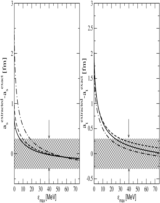
Figure 2: Dependence of the extracted scattering lengths on the value of the upper limit of integration, $\epsilon_{max}$. Shown is the difference from the exact results for the spin singlet scattering length $a_{s}$ (left panel) and the spin triplet scattering length $a_{t}$ (right panel). The solid and the dot–dashed line correspond respectively to model NSC97a and NSC97f of Ref. [5] and the dashed one corresponds to the $YN$ model of Ref. [6]. The shaded area indicates the estimated error of the proposed method and the arrows indicate the value for $\epsilon_{max}$ as estimated based on scale arguments.

2.3 Relevant scales and error estimates

The next step is to estimate an appropriate range of values for $m_{max}^{2}$ as well as the systematic uncertainty of the method. Naturally, $m_{max}^{2}$ has to be large enough to allow resolution of the relevant structures of the final state interaction. (Note that $m_{max}^{2}\to m_{0}^{2}$ leads to a vanishing value for the scattering length, c.f. Eq. (2).) On the other hand it should be as small as possible in order to ensure that the $\Lambda N$ system is still produced predominantly in an $S$–wave but also, as mentioned, to avoid the explicit inclusion of further right-hand cuts such as the one resulting from the opening of the $\Sigma N$ channel.

Eq. (10) suggests that we should choose $m_{max}^{2}$ large enough to allow values of $p^{\prime}$ such that $ap^{\prime}\sim 1$. Thus, for non–relativistic kinematics, we find $m_{max}^{2}\sim m_{0}^{2}(1+1/(\mu m_{0}a^{2}))$. A more transparent quantity is $\epsilon_{max}$ defined by

$$\epsilon_{max}=m_{max}-m_{0}\simeq\frac{1}{2\mu a^{2}}\ ,$$

i.e. the maximum kinetic energy of the $\Lambda N$ system for which it contributes to the integral of Eq. (2). For $a\sim 1$ fm we get $\epsilon_{max}\sim$ 40 MeV. This is well below the $\Sigma N$ threshold which corresponds to an energy of 75 MeV and the threshold for the $\pi\Lambda N$ channel which is at 140 MeV.

Let us now estimate the uncertainty. Except for the neglect of the kaon–baryon interactions, Eq. (17) is exact. Therefore $\delta a^{(th)}$ – the theoretical uncertainty of the scattering length extracted using Eq. (2) – is given by the integral

$$\delta a^{(th)} = -\lim_{{m}^{2}\to m_{0}^{2}}\frac{1}{2\pi}\left(\frac{m_{\Lambda}+m_{N}}{\sqrt{m_{\Lambda}m_{N}}}\right)$$ (18)

$$\qquad\times{\bf P}\int_{m_{0}^{2}}^{m_{max}^{2}}\frac{\log{|\tilde{\Phi}(m_{max}^{2},m^{\prime}\,{}^{2})|^{2}}}{\sqrt{m^{\prime}\,{}^{2}-m_{0}^{2}}(m^{\prime}\,{}^{2}-m^{2})}\sqrt{\frac{m_{max}^{2}-m^{2}}{m_{max}^{2}-m^{\prime}\,{}^{2}}}dm^{\prime}\,{}^{2}.$$

Since $\log{|\tilde{\Phi}(m_{max}^{2},m^{2})|^{2}}=\log{|\Phi(m^{2})|^{2}}+\log{|\Phi_{m_{max}^{2}}(m^{2})|^{2}}$, we may write $\delta a^{(th)}=\delta a^{(lhc)}+\delta a^{m_{max}}$, where the former, determined by $\Phi(m^{2})$, is controlled by the left hand cuts and the latter, determined by $\Phi_{m_{max}^{2}}(m^{2})$, by the large energy behavior of the $\Lambda N$ scattering phase shifts. The closest left hand singularity is that introduced by the exchange of light mesons ($\pi$ and $K$) in the production operator and it is governed by the momentum transfer. Up to an irrelevant overall constant, we may therefore estimate the variation of $\Phi\sim 1+\kappa(p^{\prime}/p)^{2}$, where we assume $\kappa$ to be of the order of 1. Evaluation of the integral (18) then gives

$$\delta a^{(lhc)}\sim\kappa(p^{\prime}_{max}/p^{2})\sim 0.05\ \mbox{fm}\ .$$

Here we used $p^{\prime}_{max}\,{}^{2}=2\mu\epsilon_{max}$ with $\epsilon_{max}\sim 40$ MeV and $p\sim 900$ MeV, where the latter is the center-of-mass momentum in the initial $NN$ or $\gamma d$ state that corresponds to the $K\Lambda N$ threshold energy. Concerning $\delta a^{m_{max}}$ we start from the definition of $\Phi_{m_{max}^{2}}(m^{2})$ in Eq. (15) from which one easily derives

$$|\delta a^{m_{max}}|=\frac{2}{\pi p^{\prime}_{max}}\left|\int_{0}^{\infty}\frac{\delta(y)dy}{(1+y^{2})^{(3/2)}}\right|\leq\frac{2}{\pi p^{\prime}_{max}}|\delta_{max}|\ ,$$ (19)

where $y^{2}=(m^{2}-m_{max}^{2})/(m_{max}^{2}-m_{0}^{2})$. Thus, in order to obtain an estimate for $\delta a^{m_{max}}$, we need to make an assumption about the maximum value of the elastic $\Lambda N$ phase for $m^{2}\geq m_{max}^{2}$. In addition, it is important to note that the denominator in the integral appearing in Eq. (19) strongly suppresses large values of $y$. Since for none of the considered $YN$ models [2, 3, 4, 5, 6] does $\delta_{max}$ exceed 0.4 rad, we arrive at the estimate $\delta a^{m_{max}}\sim 0.2$ fm. Note that when using the phase shifts as given by those models directly in the integral, the value for $\delta a^{m_{max}}$ is significantly smaller, since for all models considered the phase changes sign at energies above $m_{max}^{2}$. Combining the two error estimates, we conclude

$$\delta a\lesssim 0.3\ \mbox{fm}\ .$$

Another source of uncertainty comes from possible final state interactions in the $KN$ and $K\Lambda$ systems. Their effects have been neglected in our considerations so far for a good reason: their influence is to be energy dependent and therefore no general estimate for the error induced by them can be given. For example, baryon resonances are expected to have a significant influence on the production cross sections [36]. However, it is possible to examine the influence of the meson–baryon interactions experimentally, namely through a Dalitz plot analysis. This allows to see directly, if the area where the $\Lambda N$ interaction is dominant is isolated or is overlapping with resonance structures [37]. In addition, to quantify the possible influence of the meson–baryon interactions on the resulting scattering lengths, the extraction procedure proposed above is to be performed at two or more different beam energies. If the obtained scattering lengths agree, we can take this as a verification that the result is not distorted by the interactions in the other subsystems because their influence necessarily depends on the total energy, whereas the extraction procedure does not.

3 Test of the method: comparison to model calculations

The most obvious way to test Eq. (2) would be to apply it to reactions where the involved scattering lengths are known as it is the case for any large momentum transfer reaction with a two nucleon final state. Unfortunately, as far as we know there are is no experimental information on $nn$ or $pn$ mass spectra with sufficient resolution to allow the application of Eq. (2). For existing invariant mass spectra with a $pp$ final state, as given, e.g., in Ref. [38] for the reaction $pp\to pp\pi^{0}$, our formula is not applicable due to the presence of the Coulomb interaction that strongly distorts the invariant mass spectrum exactly in the regime of interest. Moreover, one has to keep in mind that the authors of Ref. [38] were forced to assume already a particular $m^{2}$ dependence of the outgoing $pp$ system at small values of $m^{2}$ for their analysis because of the limited detector acceptance. Thus, a test with those data would not be conclusive, anyway.

Therefore, we chose a different strategy in order to test our method. We apply Eq. (2) to the results of a microscopic model for the reaction $pp\to K^{+}p\Lambda$ [35]. (We expect that application to the reaction $\gamma d\to K^{+}n\Lambda$ gives similar results.) In this model the $K$ production is described by the so-called $\pi$ and $K$ exchange mechanisms. Thereby a meson ($\pi$ or $K$) is first produced from one of the nucleons and then rescattered on the other nucleon before it is emitted (cf. Ref. [35] for details). The rescattering amplitudes ($\pi N\to KY$, $KN\to KN$) are parameterized by their on-shell values at threshold. The $YN$ final state interaction, however, is included without approximation. Specifically, the coupling of the $\Lambda N$ to the $\Sigma N$ system is treated with its full complexity. For the present test calculations we used all the $YN$ models of Ref. [5] as well as the $YN$ model of Ref. [6]. Thus, the test calculation will allow us to see a possible influence of the $\Sigma N$ channel as well as that of the left hand singularities induced by the production operator. In addition, we can study the effect of the value of the upper integration limit $m_{max}^{2}$ or, equivalently, $\epsilon_{max}$ on the scattering length extracted.

We now proceed as follows: we calculate the invariant mass spectra needed as input for Eq. (2), utilizing the $YN$ models mentioned above. Then we use that equation to extract the scattering lengths from the invariant mass plots. In Fig. 2 the difference between the extracted scattering length and the exact one is shown as a function of $\epsilon_{max}$ for several $YN$ models. The direction of kaon emission was chosen as 90 degees in the center of mass. Considered are the two “extreme” models of Ref. [5], namely NSC97a, with singlet scattering length $a_{s}=-0.71$ fm and triplet scattering length $a_{t}=-2.18$ fm, and NSC97f ($a_{s}=-2.51$ fm and $a_{t}=-1.75$ fm), and the new Jülich model ($a_{s}=-1.02$ fm and $a_{t}=-1.89$ fm). The last was included here because it should have a significantly different short range behavior compared to the other two. As can be seen from the figure, for $\epsilon_{max}\simeq$ 40 MeV in all cases the extracted value for the scattering length does not deviate from the exact one by more than the previously estimated 0.3 fm, as is indicted by the shaded area in Fig. 2. This is in accordance with the error estimates given in the previous section, where $\epsilon_{max}\sim 40$ MeV – in the figure highlighted by the arrows – was deduced from quite general arguments. In addition, this investigation also suggests that the $\Sigma N$ cuts, included in the model without approximation, do not play a significant role in the determination of the scattering length.

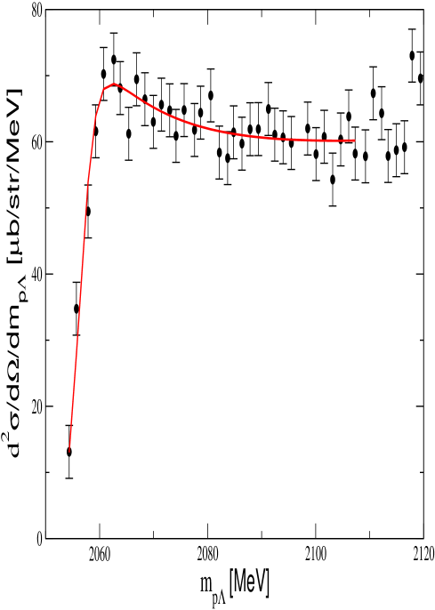
Figure 3: $pp\to K^{+}X$ inclusive missing mass spectrum at $T_{p}$ = 2.3 Gev for kaon laboratory scattering angles $\theta^{L}_{K}$ = 10$\pm 2^{o}$ [39]. The solid line is our fit as described in the text. Note that the scattering length extracted is insensitive to the parameterization of the data used (see Appendix for details).

4 Application to existing data

As was stressed in the derivation, Eq. (2) can be applied only to observables (cross sections) that are dominated by a single partial wave. This is indeed the case for specific polarization observables for near-threshold kinematics as we show in the appendix B for the reaction $pp\to NK\Lambda$. Unfortunately, at present no suitable polarization data are available that could be used for a practical application of our formalism. Thus, in order to demonstrate the potential of the proposed method, we will apply it to the unpolarized data for the reaction $pp\to K^{+}X$ measured at the SPES4 facility in Saclay [39]. Obviously, since we only consider the small invariant mass tail of the double differential cross section, we automatically project on the $p\Lambda$ $S$–waves. The data, however, still contains contributions from both possible final spin states – spin triplet as well as spin singlet. Thus the scattering length extracted from those data is an effective value that averages over the spin-dependence of the $p\Lambda$ interaction in the final state and also over the spin dependence of the production mechanism with unknown weightings. It does not allow any concrete conclusions on the elementary $p\Lambda$ (${}^{1}S_{0}$ or ${}^{3}S_{1}$) scattering lengths. We should mention, however, that some model calculations of the reaction $pp\to K^{+}p\Lambda$ [35, 40] indicate that the production mechanism could be dominated by the spin-triplet configuration. If this is indeed the case then the production process would act like a spin filter and the scattering length extracted from the Saclay data could then be close to the one for the $p\Lambda$ ${}^{3}S_{1}$ partial wave.

For our exemplary calculation we use specifically the data on the $pp\to K^{+}X$ inclusive missing mass spectrum at $T_{p}$ = 2.3 GeV for kaon laboratory scattering angles $\theta^{L}_{K}$ = 10$\pm 2^{o}$ [39] (cf. Fig. 3). For convenience we represent those data in terms of simple analytical functions (the result of the best fit is shown as the solid line in the figure) as described in appendix A. Please note, however, that the advantage of the proposed method is that the scattering length extracted is independent of the particular analytical parameterization employed; one can even use the data directly. In particular we do not need to assume that the elastic $\Lambda N$ interaction can be represented by the first two terms of an effective range expansion. The analytical representation of the data is then used to evaluate the corresponding scattering length utilizing Eq. (2). Details of the fitting as well as how we extract the uncertainty in the scattering length can be found in the appendix.

We find a scattering length of $(-1.5\pm 0.15\pm 0.3)$ fm, where the first error corresponds to the uncertainty from the data and the second one is the theoretical uncertainty discussed previously. Thus, already in the case of an experimental resolution of about 2 MeV the experimental error is smaller than the theoretical one.

5 Summary

In this paper we presented a formalism that allows one to relate spectra from large-momentum transfer reactions, such as $pp\to K^{+}p\Lambda$ or $\gamma d\to K^{+}n\Lambda$, directly to the scattering length of the interaction of the final state particles. We estimated the theoretical error of the analysis to be less than 0.3 fm. This estimate was confirmed by comparing results obtained with the proposed formalism to those of microscopic model calculations for the specific reaction $pp\to K^{+}\Lambda p$.

The formalism can be applied only to observables (cross sections) that are dominated by a single partial wave. This requirement is fulfilled by specific polarization observables for $\Lambda N$ invariant masses near threshold as we show in the appendix B for the reaction $pp\to NK\Lambda$. Corresponding experiments require a polarized beam or target in order to pin down the spin-triplet scattering length and polarized beam and target for determining also the spin-singlet scattering length.

Since at present no suitable polarization data are available we demonstrated the potential of the proposed method by applying it to unpolarized data from the reaction $pp\to K^{+}X$ measured at the SPES4 facility in Saclay [39]. Thereby a scattering length of $(-1.5\pm 0.15\pm 0.3)$ fm was extracted. This more academic exercise demonstrates that the resolution of 2 MeV of the SPES4 spectrometer is already sufficient to obtain scattering lengths with an experimental error of less than 0.2 fm. Such an accuracy would be already an improvement over the present situation.

The method of extraction of the $YN$ scattering lengths discussed here should be viewed as an alternative method to proposed analyses of other reaction channels involving the $YN$ system like $K^{-}d\to\gamma n\Lambda$. The assumptions that go into the analyses are very different and therefore carrying out both analyses is useful in order to explore the systematic uncertainties.

Acknowledgments

We thank A. Kudryavtsev for stimulating discussion and J. Durso for critical comments and a careful reading of the manuscript. We are grateful to M. P. Rekalo and E. Tomasi-Gustafsson for inspiring and educating discussions about spin observables.

Appendix A Method of the Analysis

In order to evaluate the integral in Eq. (2) for the experimental results of Ref. [39] we first fit the data utilizing the following parameterization for the amplitude squared (c.f. Eq. (17)):

$$|A(m)|^{2}=\exp{\left[C_{0}+\frac{C_{1}^{2}}{(m^{2}-C_{2}^{2})}\right]}.$$ (20)

The advantage of such a parameterization is that the integral in Eq. (2) can be calculated analytically and one gets for the scattering length

$$a(C_{1},C_{2})=-\frac{1}{2}C_{1}^{2}\sqrt{\left(\frac{m_{0}^{2}}{m_{N}m_{\Lambda}}\right)\frac{(m_{max}^{2}-m_{0}^{2})}{(m_{max}^{2}-C_{2}^{2})(m_{0}^{2}-C_{2}^{2})^{3}}}.$$ (21)

One can extend Eq. (20) easily by including in the exponent additional terms such as $C_{3}^{2}/(m^{2}-C_{4}^{2})$ if required for a satisfactory analytical representation of the data. The accuracy of the presently available experimental results, however, did not necessitate such an extension, for already the form given in Eq. (20) ensured a $\chi^{2}$ per degree of freedom of less than 1.

In Ref. [41] it is stressed that there is a calibration uncertainty in the data of Ref. [39]. The actual value of this uncertainty was determined by including as a free parameter a shift $\Delta m$ in the fitting procedure. In this way a value of $\Delta m=1.17$ MeV was found. We use the same value. In addition, the finite resolution of the detector $\sigma_{m}=2$ MeV has to be taken into account. Thus the function

$$\frac{d^{2}\sigma(m)}{dmd\Omega_{K}}=\int_{-\infty}^{\infty}\left(\frac{d^{2}\sigma(m^{\prime})}{dm^{\prime}d\Omega_{K}}\right)_{0}\frac{1}{\sqrt{2\pi}\sigma_{m}}\exp{\left[\frac{-(m-m^{\prime}-\Delta m)^{2}}{\sigma_{m}}\right]}dm^{\prime}\ ,$$ (22)

is to be compared to the data, where $(d^{2}\sigma(m^{\prime})/(dm^{\prime}d\Omega_{K}))_{0}$ is calculated from the amplitude Eq. (20).

The probability for the data to occur under the assumption that the cross section given in Eq. (22) is true is given by the Likelihood function. Here we assume the data distribution to be Gaussian:

$$\mathcal{L}(\{\mbox{data}\}|C0,C1,C2;I)\propto\exp{\left[-\frac{1}{2}\chi^{2}(C_{0},C_{1},C_{2})\right]}\ ,$$ (23)

where the standard $\chi^{2}$ function appears in the exponent. The letter $I$ that appears in the argument of $\mathcal{L}$ is meant to remind the reader that some assumptions had to be made in order to write down Eq. (23).

The distribution of interest to us is the probability distribution of the scattering length $\mathcal{L}(a|\{\mbox{data}\};I)$, given the data, that can be written as [42]

$$\mathcal{L}(a|\{\mbox{data}\};I) =$$ (24)

$$\mathcal{N} \int\prod_{i}dC_{i}\mathcal{L}(\{\mbox{data}\}|C0,C1,C2;I)\delta(a-a(C_{1},C_{2}))\ ,$$

where $\mathcal{N}$ is a normalization constant to be fixed through $\int\mathcal{L}(a)da=1$ and $a(C_{1},C_{2})$ is given in Eq. (21).

It turns out that the Likelihood function of Eq. (23) is strongly peaked. For the numerical evaluation of Eq. (24) we therefore linearize the individual terms with respect to the parameters $C_{i}$. Within this linear approximation the resulting probability density function $\mathcal{L}(a)$ also takes a Gaussian form. To test that there is no significant dependence of the result on the parameterization used for the data we also used the Jost function in the analysis. The results for the scattering lengths determined with the two different methods agreed within the statistical uncertainty.

Appendix B Spin dependence of the reaction $pp\to\Lambda pK^{+}$

The aim of this appendix is to show how polarization measurements for the reaction $pp\to\Lambda pK^{+}$ can be used to disentangle the spin dependence of the production cross section.

In terms of the so called Cartesian polarization observables, the spin–dependent cross section can be written as [43]

$$\sigma(\xi,\vec{P}_{b},\vec{P}_{t},\vec{P}_{f}) = \sigma_{0}(\xi)\left[1+\sum_{i}((P_{b})_{i}A_{i0}(\xi)+(P_{f})_{i}D_{0i}(\xi))\right.$$ (25)

$$\left.\phantom{\sigma_{0}(\xi)[1}\ +\sum_{ij}(P_{b})_{i}(P_{t})_{j}A_{ij}(\xi)+...\right]$$

where $\sigma_{0}(\xi)$ is the unpolarized differential cross section, the labels $i,j$ and $k$ can be either $x,y$ or $z$, and $P_{b}$, $P_{t}$ and $P_{f}$ denote the polarization vector of beam, target and one of the final state particles, respectively. All quantities are functions of the 5 dimensional phase space, abbreviated as $\xi$. The observables shown explicitly in Eq. (25) include the beam analysing powers $A_{i0}$, the corresponding quantities for the final state polarization $D_{0i}$, and the spin correlation coefficients $A_{ij}$. Polarization observables not relevant for this work are not shown explicitly. All those observables that can be defined by just exchanging $\vec{P}_{b}$ and $\vec{P}_{t}$, such as the target analyzing power $A_{0i}$, are not shown explicitly.

The most general form of the transition matrix element may be written as [37]

$${\mathcal{M}}=H({\mathcal{I}}\,{\mathcal{I}\,^{\prime}})+i\vec{Q}\cdot(\vec{S}\,{\mathcal{I}^{\prime}})+i\vec{A}\cdot(\vec{S}\,^{\prime}\,{\mathcal{I}})+(S_{i}\,S_{j}\,^{\prime})B_{ij}\ ,$$ (26)

where $\vec{S}=\left(\chi_{2}^{T}\sigma_{y}\vec{\sigma}\chi_{1}\right)$ and $\vec{S}\,^{\prime}=\left(\chi_{4}^{\dagger}\vec{\sigma}\sigma_{y}(\chi_{3}^{T})^{\dagger}\right)$ are to be used for spin triplet initial and final states, respectively, and ${\mathcal{I}}=\left(\chi_{2}^{T}\sigma_{y}\chi_{1}\right)$ and ${\mathcal{I}\,^{\prime}}=\left(\chi_{4}^{\dagger}\sigma_{y}(\chi_{3}^{T})^{\dagger}\right)$ are to be used for the corresponding spin singlet states. Here it is assumed that the outgoing baryons are non relativistic, as is the case for the kinematics considered.

Figure 4: The kaon momentum $\vec{k}$ plotted in the coordinate system used; the $z$–axis is along the beam direction.

Given this form it is straight forward to evaluate the expression for the various observables. E.g.

$$4\sigma_{0} = |H|^{2}+|Q_{m}|^{2}+|A_{m}|^{2}+|B_{mn}|^{2}\,,$$ (27)

$$4A_{0i}\sigma_{0} = i\epsilon_{ikn}\left(Q_{k}^{*}Q_{n}+B_{km}^{*}B_{nm}\right)+2\mbox{Im}\left(B_{im}^{*}A_{m}-Q_{i}^{*}H\right)\,,$$ (28)

$$4D_{0i}\sigma_{0} = -i\epsilon_{ikn}\left(A_{k}^{*}A_{n}+B_{mk}^{*}B_{mn}\right)-2\mbox{Im}\left(B_{mi}^{*}Q_{m}-A_{i}^{*}H\right)\,,$$ (29)

$$4A_{ii}\sigma_{0} = -|H|^{2}+|Q_{m}|^{2}-|A_{m}|^{2}+|B_{mn}|^{2}-2|Q_{i}|^{2}-2|B_{im}|^{2}\,,$$ (30)

where the indices $m$, $k$ and $n$ are to be summed. By definition, the spin triplet final state amplitudes contribute to $A$ and $B$ only, whereas the spin singlet amplitudes contribute to $H$ and $Q$. By definition, the spin triplet states interfere with the spin singlet states only, if the final state polarization is measured. In the examples given above this is the case for $D_{0i}$ only. This simplifies the analysis considerably. Eq. (2) needs as input only those cross sections that have low relative energies, where we can safely assume the $\Lambda N$ system to be in an $S$–wave. Thus, in order to construct the most general transition amplitude under this condition, we need to express the quantities $H$, $\vec{Q}$, $\vec{A}$ as well as $B_{ij}$ in terms of the vectors $\vec{k}$ (the momentum of the kaon) and $\vec{p}$ (the momentum of the initial protons)—c.f. Fig. 4. The Pauli Principle demands for a proton–proton initial state, that $\vec{S}$ appears with odd powers of $\vec{p}$ and terms that do not contain $\vec{S}$ appear with even powers of $\vec{p}$. Correspondingly, due to parity conservation these amplitudes need to be even and odd in $\vec{k}$ respectively, since the kaon has a negative intrinsic parity. We may therefore write

$$H = 0\,,$$

$$\vec{Q} = s_{1}(\vec{k}\cdot\hat{p})\vec{k}+s_{2}\hat{p}\,,$$

$$\vec{A} = t_{1}\hat{p}(\hat{p}\cdot\vec{k})+t_{2}\vec{k}\,,$$

$$B_{ij} = \epsilon_{ijk}\left(t_{3}k_{k}(\vec{k}\cdot\hat{p})+t_{4}\hat{p}_{k}\right)+(\vec{k}\times\hat{p})_{i}\left(t_{5}k_{j}+t_{6}(\hat{p}\cdot\vec{k})\hat{p}_{j}\right)\,,$$ (31)

where $\hat{p}=\vec{p}/|\vec{p}|$. The amplitudes $s_{i}$ and $t_{i}$ appearing in the above equations are functions of $p^{2}$, $k^{2}$ and $(\vec{k}\cdot\vec{p})^{2}$. Now we want to identify observables that either depend only on (some of) the $s_{i}$ and thus are sensitive to the spin singlet $\Lambda N$ interaction only or on (some of) the $t_{i}$ and thus are sensitive to the spin triplet $\Lambda N$ interaction only. It should be stressed in this context that it is entirely due to the relation $H=0$ – a direct consequence of the selection rules – that one can disentangle the spin triplet and the spin singlet channel without making assumptions about the kaon partial wave, as was first observed in Ref. [44].

Using Eqs. (31) all observables can be expressed in terms of the amplitudes $s_{i}$ and $t_{i}$, where the former correspond to a spin singlet $YN$ pair in the final state, while the latter correspond to a spin triplet pair. We find

$$A_{0i}\sigma_{0}=\frac{1}{2}(\vec{k}\times\hat{p})_{i}\left(\alpha+\beta(\vec{k}\cdot\hat{p})+\gamma(\vec{k}\cdot\hat{p})^{2}\right)$$ (32)

where

$$\alpha = \mbox{Im}(t_{4}^{*}t_{2}+t_{5}^{*}t_{2}\vec{k}\,^{2})\ ,$$ (33)

$$\beta = \mbox{Im}(t_{4}^{*}t_{3}+s_{2}^{*}s_{1})\ ,$$ (34)

$$\gamma = \mbox{Im}(t_{5}^{*}t_{1}+t_{6}^{*}t_{1}+t_{6}^{*}t_{2}-t_{3}^{*}t_{1})\ .$$ (35)

We may express the results in the coordinate system defined by the beam along the $z$ axis and the $x$ and $y$ directions through the polarizations (c.f. Fig. 4). Then we find for the analysing power

$$A_{0y}\sigma_{0} = -\frac{1}{4}k^{2}\beta\sin(2\theta)\cos(\phi)$$ (36)

$$\ \ \ \ \ +\sin(\theta)\cos(\phi)\mbox{(spin triplet only)}\ ,$$

where we used $(\hat{p}\times\vec{k})_{y}=k\sin(\theta)\cos(\phi)$ and $\hat{p}\cdot\vec{k}=k\cos(\theta)$. Thus, the contributions from all those partial waves where the final $\Lambda N$ system is in an ${}^{1}S_{0}$ state vanish when the kaon goes out in the $xy$–plain. In addition, the term proportional to $\beta$ is the only one that is odd in $\cos(\theta)$, and thus any integration with respect to the angle $\theta$ of $A_{0y}\sigma_{0}$ symmetric around $\pi/2$ removes any spin singlet contribution from the observable. Please note that for any given energy it should be checked whether the range of angular integration performed is consistent with the requirement that the reaction was dominated by a large momentum transfer – kaon emission at 90 degrees maximizes the momentum transfer and thus minimizes the error in the extraction method.

Analogously one can show for the combination $(1-A_{xx})\sigma_{0}$ that

$$(1-A_{xx})\sigma_{0} = \frac{1}{2}\left(|\vec{A}|^{2}+|Q_{x}|^{2}+|B_{xm}|^{2}\right)$$ (37)

$$= \frac{1}{8}k^{4}|s_{1}|^{2}\sin^{2}(2\theta)\cos^{2}(\phi)+\mbox{(spin triplet only)}\ ,$$

i.e. that it also allows to isolate the amplitudes with the $YN$ system in the spin triplet. Furthermore,

$$(1+A_{xx}+A_{yy}-A_{zz})\sigma_{0}$$ (38)

$$\!\!\!\!\!\!\!\!\!\!\!\!\!\!\!\!\!\!\!\!\!\!\!\!\!\!\!\!\!\!\!\!\!=|Q_{z}|^{2}+|B_{zm}|^{2}$$

$$\!\!\!\!\!\!\!\!\!\!\!\!\!\!\!\!\!\!\!\!\!\!\!\!\!\!\!\!\!\!\!\!\!=\frac{1}{4}k^{4}|t_{3}|^{4}\sin^{2}(2\theta)+\mbox{(spin singlet only)}\$$

and therefore allows to isolate the spin singlet amplitudes. (Note that in both cases a summation over $m$ is to be performed.) Thus, for all those partial waves where the final $YN$ system is in the ${}^{1}S_{0}$ final state, $(1-A_{xx})$ vanishes, when the kaon goes out in the $yz$– or in the $xy$–plain and for all those partial waves where the final $YN$ system is in the ${}^{3}S_{1}$ final state, $(1+A_{xx}+A_{yy}-A_{zz})$ vanishes, when the kaon goes out in the $xy$–plain or in forward direction. These results hold independent of the orbital angular momentum of the kaon.

So far we assumed that higher partial waves of the $\Lambda N$ system do not play a role – since we restricted ourselves to small relative energies. However, it is also possible to check this experimentally. First of all the angular distribution of the $YN$ system $d\sigma/d\Omega_{p^{\prime}}$, where $\vec{p}\,^{\prime}$ is the relative momentum of the two outgoing baryons, needs to be flat. However, in the presence of spins even flat angular distributions can stem from higher partial waves [45]. To exclude this possibility the $\Lambda$ polarization can be used. For this test we need an observable that vanishes in the absence of higher $\Lambda N$ partial waves. The easiest choice here is $D_{0i}$. It is straight forward to show that

$$D_{0i}\propto(\vec{p}\times\vec{k})_{i}\ ,$$

as long as there are only $S$ waves in the $\Lambda N$ system. Therefore, in the absence of higher partial waves in the $YN$ system $D_{0z}$ has to vanish.

References

- [1] C.B. Dover and A. Gal, Prog. Part. Nucl. Phys. 12, 171 (1984).
- [2] P.M.M. Maessen, Th.A. Rijken, and J.J. de Swart, Phys. Rev. C 40, 2226 (1989).
- [3] B. Holzenkamp, K. Holinde, and J. Speth, Nucl. Phys. A500, 485 (1989).
- [4] A. Reuber, K. Holinde, and J. Speth, Nucl. Phys. A570, 543 (1994).
- [5] Th.A. Rijken, V.G. Stoks, and Y. Yamamoto, Phys. Rev. C 59, 21 (1999).
- [6] J. Haidenbauer, W. Melnitchouk, and J. Speth, AIP Conf. Proc. 603, 421 (2001), nucl-th/0108062.
- [7] G. Alexander et al., Phys. Lett. 19, 715 (1966); B. Sechi-Zorn et al., Phys. Rev. 175, 1735 (1968).
- [8] G. Alexander et al., Phys. Rev. 173, 1452 (1968);
- [9] H.G. Dosch et al., Phys. Lett. 21, 236 (1966); R. Engelmann et al., Phys. Lett. 21, 587 (1966); F. Eisele et al., Phys. Lett. 37B, 204 (1971).
- [10] J.K. Ahn et al., Nucl. Phys. A648, 263 (1999); Y. Kondo et al., Nucl. Phys. A676, 371 (2000); T. Kadowaki et al., Eur. Phys. J. A 15, 295 (2002).
- [11] B.F. Gibson et al., BNL Report No. 18335, 1973.
- [12] K.P. Gall et al., Phys. Rev. C 42, R475 (1990).
- [13] A.I. Akhiezer, G.I. Gakh, A.P. Rekalo, and M.P. Rekalo, Sov. J. Nucl. Phys. 27, 115 (1978).
- [14] R.L. Workman and H.W. Fearing, Phys. Rev. C 41, 1688 (1990).
- [15] W.R. Gibbs et al., Phys. Rev. C 61, 064003 (2000).
- [16] H.H. Tan, Phys. Rev. Lett. 23, 395 (1969).
- [17] J. T. Balewski et al., Phys. Lett. B 420, 211 (1998); S. Sewerin et al., Phys. Rev. Lett. 83, 682 (1999).
- [18] R. Bilger et al., Phys. Lett. B 420, 217 (1998).
- [19] J. T. Balewski et al., Eur. Phys. J. A 2, 99 (1998).
- [20] F.M. Renard and Y. Renard, Nucl. Phys. B1, 389 (1967).
- [21] B. Mecking et al., CEBAF proposal PR-89-045 (1989).
- [22] R.A. Adelseck and L.E. Wright, Phys. Rev. C 39, 580 (1989).
- [23] X. Li and L.E. Wright, J. Phys. G 17, 1127 (1991).
- [24] H. Yamamura, K. Miyagawa, T. Mart, C. Bennhold, H. Haberzettl, and W. Glöckle, Phys. Rev. C 61, 014001 (1999).
- [25] M. Goldberger and K. Watson, Collision Theory (Wiley, New York 1964).
- [26] K. Watson, Phys. Rev. 88, 1163 (1952); A.B. Migdal, Sov. Phys. JETP 1, 2 (1955).
- [27] H.O. Meyer et al., Phys. Rev. Lett. 65, 2846 (1990); H.O. Meyer et al., Nucl. Phys. A539, 633 (1992).
- [28] N. I. Muskhelishvili, Singular Integral Equations, (P. Noordhof N. V., Groningen, 1953).
- [29] R. Omnes, Nuovo Cim. 8, 316 (1958).
- [30] W. R. Frazer and J. R. Fulco, Phys. Rev. Lett. 2, 365 (1959).
- [31] M. Goldberger and K.M. Watson, Collision Theory (Wiley, New York, 1964).
- [32] B. V. Geshkenbein, Yad. Fiz. 9, 1232 (1969) [Sov. J. Nucl. Phys. 9, 720 (1969)].
- [33] B. V. Geshkenbein, Phys. Rev. D 61, 033009 (2000).
- [34] G. Faeldt and C. Wilkin, Phys. Lett. B 354 (1995) 20.
- [35] A. Gasparian, J. Haidenbauer, C. Hanhart, L. Kondratyuk and J. Speth, Phys. Lett. B 480, 273 (2000).
- [36] R. Shyam, G. Penner, and U. Mosel, Phys. Rev. C 63, 022202 (2001).
- [37] C. Hanhart, submitted to Phys. Reports.
- [38] R. Bilger et al., Nucl. Phys. A 693 (2001) 633.
- [39] R. Siebert et al., Nucl. Phys. A567, 819 (1994).
- [40] J. M. Laget, Phys. Lett. B 259 (1991) 24.
- [41] F. Hinterberger and A. Sibirtsev, in preparation.
- [42] For a very pedagogical introduction see D. S. Sivia, Data Analysis/ A Bayesian Tutorial (Oxford University Press Inc., New York, 1996).
- [43] H. O. Meyer et al., Phys. Rev. C 63 (2001) 064002.
- [44] S.E. Vigdor, in Flavour and Spin in Hadronic and Electromagnetic Interactions, ed. F. Balestra et al. (Italian Physical Society, Bologna, 1993), p. 317.
- [45] K. Nakayama, J. Haidenbauer, C. Hanhart and J. Speth, Phys. Rev. C 68 (2003) 045201.