PCCF-RI-03-09

ADP-03-135/T570

${\rm ECT}^{*}$-03-30

Simulation Methods of the Processes $\boldsymbol{B\to{\pi}^{+}{\pi}^{-}V}$ Including $\boldsymbol{\rho^{0}-\omega}$ Mixing Effects

Z.J. Ajaltouni¹, O. Leitner², P. Perret¹, C. Rimbault¹,

A.W. Thomas³

¹ Laboratoire de Physique Corpusculaire de Clermont-Ferrand
IN2P3/CNRS Université Blaise Pascal
F-63177 Aubière Cedex France
² ${\rm{ECT}}^{*}$, Strada delle Tabarelle, 286,
38050 Villazzano (Trento), Italy
³ Department of Physics and Mathematical Physics and
Special Research Centre for the Subatomic Structure of Matter,
University of Adelaide, Adelaide 5005, Australia
Talk presented at the
CERN Workshop on Event Generators
CERN, GENEVA, JULY 22-26, 2003

Simulation methods for the decays $B\to{\pi}^{+}{\pi}^{-}V$, where $V$ is a $1^{--}$ vector-meson, are presented in detail. Emphasis is put on the use of the helicity formalism and the use of effective Lagrangians. We show the importance of ${{\rho}^{0}}-{\omega}$ mixing in enhancing the direct $CP$ violation (DCPV) when the pion-pion invariant mass is near the mass of the $\omega$.

1 Introduction

In the framework of the LHCb experiment devoted to the search for $CP$ violation and rare $B$ decays, special care is given to the $B$ decays into two vector mesons, $B\to V_{1}V_{2},\ \ V_{i}=\ 1^{--}$. Physical motivations for studying these processes are numerous:

(i) Weak interaction governing the $B$ decays, the vector-mesons are polarized and their final states have specific angular distributions; which allows one to cross-check the Standard Model (SM) predictions and to perform tests of models beyond the SM.

(ii) In the special case of two neutral vector mesons with $\bar{V^{0}}=V^{0}$, the orbital angular momentum, $\ell$, the total spin $S$ and the $CP$ eigenvalues are related by the following relations:

$$\ell=\ S\ =\ 0,1,2\ \ \Longrightarrow CP\ =\ {(-1)}^{\ell}\ ,$$

which implies a mixing of different $CP$ eigenstates, leading to $CP$ non-conservation process. According to Dunietz et al [1], tests of $CP$ violation in a model independent way can be performed and severe constraints on models beyond the SM can be set.

2 Helicity formalism and its applications

Because the $B$ meson has spin $0$, the final two vector mesons, $V_{1}$ and $V_{2}$, have the same helicity ${\lambda}_{1}={\lambda}_{2}=-1,0,+1,$ and their angular distribution is isotropic in the $B$ rest frame. Let $H_{w}$ be the weak Hamiltonian which governs the $B$ decays. Any transition amplitude between the initial and final states will have the following form:

$$H_{\lambda}=\langle V_{1}{(\lambda)}V_{2}{(\lambda)}|H_{w}|B\rangle\ ,$$ (1)

where the common helicity is ${\lambda}=-1,0,+1$. Then, each vector meson $V_{i}$ will decay into two pseudo-scalar mesons, $a_{i},b_{i}$, where $a_{i}$ and $b_{i}$ can be either a pion or a kaon, and the angular distributions of $a_{i}$ and $b_{i}$ depend on the $V_{i}$ polarization.

The helicity frame of a vector-meson, $V_{i}$, is defined in the $B$ rest frame such that the direction of the Z-axis is given by its momentum ${\vec{p}_{i}}$. Schematically, the whole process gets the form:

$$B\longrightarrow V_{1}+V_{2}\longrightarrow(a_{1}+b_{1})+(a_{2}+b_{2})\ .$$

The corresponding decay amplitude, $M_{\lambda}\bigl{(}B\rightarrow\sum_{i=1}^{2}(a_{i}+b_{i})\bigr{)}$, is factorized according to the relation,

$$M_{\lambda}\bigl{(}B\rightarrow\sum_{i=1}^{2}(a_{i}+b_{i})\bigr{)}=H_{\lambda}(B\rightarrow V_{1}+V_{2})\times\prod_{i=1}^{2}A_{i}(V_{i}\rightarrow a_{i}+b_{i})\ ,$$ (2)

where the amplitudes $A_{i}(V_{i}\rightarrow a_{i}+b_{i})$ are related to the decay of the resonances $V_{i}$. The $A_{i}(V_{i}\rightarrow a_{i}+b_{i})$ are given by the following expressions:

$$A_{1}(V_{1}\rightarrow a_{1}+b_{1}) =\sum_{m_{1}=-1}^{1}c_{1}D^{1}_{\lambda,m_{1}}(0,\theta_{1},0)\ ,$$

$$A_{2}(V_{2}\rightarrow a_{2}+b_{2}) =\sum_{m_{2}=-1}^{1}c_{2}D^{1}_{\lambda,m_{2}}(\phi,\theta_{2},-\phi)\ .$$ (3)

These equalities are an illustration of the Wigner-Eckart theorem. In Eq. (2), the $c_{1}$ and $c_{2}$ coefficients represent, respectively, the dynamical decay parameters of the $V_{1}$ and $V_{2}$ resonances. The term $D^{1}_{\lambda,m_{i}}(\phi_{i},\theta_{i},-\phi_{i})$ is the Wigner rotation matrix element for a spin-1 particle and we let $\lambda{(a_{i})}$ and $\lambda{(b_{i})}$ be the respective helicities of the final particles $a_{i}$ and $b_{i}$ in the $V_{i}$ rest frame. $\theta_{1}$ is the polar angle of $a_{1}$ in the $V_{1}$ helicity frame. The decay plane of $V_{1}$ is identified with the (X-Z) plane and consequently the azimuthal angle $\phi_{1}$ is set to $0$. Similarly, $\theta_{2}$ and $\phi$ are respectively the polar and azimuthal angles of particle $a_{2}$ in the $V_{2}$ helicity frame. Finally, the coefficients $m_{i}$ are defined as: $m_{i}=\lambda(a_{i})-\lambda(b_{i})$ Our convention for the $D^{1}_{\lambda,m_{i}}(\alpha,\beta,\gamma)$ matrix element is given in Rose’s book [2], namely:

$$D^{1}_{\lambda,m_{i}}(\alpha,\beta,\gamma)=\exp[-i(\lambda\alpha+m_{i}\gamma)]\;d^{1}_{\lambda,m_{i}}(\beta)\ .$$ (4)

The most general form of the decay amplitude ${\cal M}\bigl{(}B\rightarrow\sum_{i=1}^{2}(a_{i}+b_{i})\bigr{)}$ is a linear superposition of the previous amplitudes $M_{\lambda}\bigl{(}B\rightarrow\sum_{i=1}^{2}(a_{i}+b_{i})\bigr{)}$ denoted by:

$${\cal M}\bigl{(}B\rightarrow\sum_{i=1}^{2}(a_{i}+b_{i})\bigr{)}=\sum_{\lambda}M_{\lambda}\bigl{(}B\rightarrow\sum_{i=1}^{2}(a_{i}+b_{i})\bigr{)}\ .$$ (5)

The decay width, $\Gamma{(B\rightarrow V_{1}V_{2})}$, can be computed by taking the square of the modulus, $\Bigl{|}{\cal M}\bigl{(}B\rightarrow\sum_{i=1}^{2}(a_{i}+b_{i})\bigr{)}\Bigr{|}$, which involves the three kinematic parameters, $\theta_{1},\theta_{2}$ and $\phi$. This leads to the following general expression:

$$d^{3}{\Gamma}(B\rightarrow V_{1}V_{2})\propto\Bigl{|}\sum_{\lambda}M_{\lambda}\bigl{(}B\rightarrow\sum_{i=1}^{2}(a_{i}+b_{i})\bigr{)}\Bigr{|}^{2}=\sum_{\lambda,\lambda^{\prime}}h_{\lambda,\lambda^{\prime}}F_{\lambda,\lambda^{\prime}}(\theta_{1})G_{\lambda,\lambda^{\prime}}(\theta_{2},\phi)\ ,$$ (6)

which involves three density-matrices, $h_{\lambda,\lambda^{\prime}},F_{\lambda,\lambda^{\prime}}(\theta_{1})$ and $G_{\lambda,\lambda^{\prime}}(\theta_{2},\phi)$.

$\star$ The factor $h_{\lambda,\lambda^{\prime}}=H_{\lambda}H^{*}_{\lambda^{\prime}}$ is an element of the density-matrix related to the $B$ decay.
$\star$ $F_{\lambda,\lambda^{\prime}}(\theta_{1})$ represents the density-matrix of the decay $V_{1}\rightarrow a_{1}+b_{1}$.
$\star$ $G_{\lambda,\lambda^{\prime}}(\theta_{2},\phi)$ represents the density-matrix of the decay $V_{2}\rightarrow a_{2}+b_{2}$.

The analytic expression in Eq. (6) exhibits a very general form: it depends on neither the specific nature of the intermediate resonances nor their decay modes (except for the spin of the final particles).

The previous calculations are illustrated by the reaction $B^{0}\rightarrow K^{*0}{\rho}^{0}$ where $K^{*0}\rightarrow K^{+}{\pi}^{-}$ and ${\rho}^{0}\rightarrow{\pi}^{+}{\pi}^{-}$. In this channel, since all the final particles have spin zero, the coefficients $m_{1}$ and $m_{2}$, defined previously, are equal to zero. The three-fold differential width has the following form:

$$\frac{d^{3}\Gamma(B\rightarrow V_{1}V_{2})}{d(\cos\theta_{1})d(\cos\theta_{2})d\phi}\propto\bigl{(}h_{++}+h_{--}\bigr{)}{{\sin}^{2}{\theta_{1}}{\sin}^{2}{\theta_{2}}}/4+{h_{00}{\cos}^{2}{\theta_{1}}{\cos}^{2}{\theta_{2}}}\\ +\Bigl{\{}\mathscr{R}\!e{(h_{+0})}{\cos{\phi}}-\mathscr{I}\!m{(h_{+0})}{\sin{\phi}}+\mathscr{R}\!e{(h_{0-})}{\cos{\phi}}-\mathscr{I}\!m{(h_{0-})}{\sin{\phi}}\Bigr{\}}{{\sin{2\theta_{1}}}{\sin{2\theta_{2}}}}/4\\ +\Bigl{\{}\mathscr{R}\!e{(h_{+-})}{\cos{2\phi}}-\mathscr{I}\!m{(h_{+-})}{\sin{2\phi}}\Bigr{\}}{{\sin}^{2}{\theta_{1}}{\sin}^{2}{\theta_{2}}}/2\ .$$ (7)

It is worth noticing that the expression in Eq. (7) is completely symmetric in ${\theta}_{1}$ and ${\theta}_{2}$ and consequently, the angular distribution of $a_{1}$ in the $V_{1}$ frame is identical to that of $a_{2}$ in the $V_{2}$ frame. From Eq. (7) the normalized probability distribution functions (pdf) of ${\theta}_{1}$, ${\theta}_{2}$ and $\phi$ can be derived and one finds:

$$f{({\cos}{\theta}_{1,2})} ={(3h_{00}-1)}{{\cos}^{2}{\theta}_{1,2}}+{(1-h_{00})}\ ,$$

$$g{(\phi)} =1+2\;\mathscr{R}\!e{(h_{+-})}{\cos{2\phi}}-2\;\mathscr{I}\!m{(h_{+-})}{\sin{2\phi}}\ .$$ (8)

3 Final state interactions and $\boldsymbol{{{\rho}^{0}}-{\omega}}$ mixing

Hadrons produced from $B$ decays are scattered again by their mutual strong interactions, which could modify completely their final wave-function. Computations of the branching ratios $B\to{\rm{Hadrons}}$ must take account of the final state interactions (FSI) [3] which are generally divided into two regimes: perturbative and non-perturbative.

An important question arises: how to deal with the FSI in a simple and practical way in order to perform realistic and rigorous simulations?

The method which has been followed for the simulations is largely developed in the Ref. [6] and is based on the hypothesis of Naive Factorization, which can be summarized as follows:

• In the Feynman diagrams describing the $B$ decays into hadrons like tree or penguin diagrams, the soft gluons exchanged among the quark lines are neglected.

• Using the Effective Hamiltonian approach and applying the Operator product Expansion method (OPE), perturbative calculations are performed to the Wilson Coefficients (W.C.), $C_{i}$, at the Next to Leading Order (NLO) for an energy scale $\geq{m_{B}}$.

• Non-perturbative effects representing physical processes at an energy $\leq{m_{B}}$ are introduced through different form-factors.

• The color number, $N_{c}$, is no longer fixed and equal to 3. It is modified according to the following relation:

  $$\frac{1}{(N_{c}^{eff})}=\frac{1}{3}+\xi\ \ ,$$

where operator(s) ${\xi}$ describe(s) the non-factorizable effects.

Another important effect which appears in the channels $B\to{\pi}^{+}{\pi}^{-}V$ is the ${{\rho}^{0}}-{\omega}$ mixing which is an unavoidable quantum process. Indeed, the tree amplitude, $A^{T}$, and the penguin, $A^{P}$, are modified according to the following relations:

$$\langle K^{*}\pi^{-}\pi^{+}|H^{T}|B\rangle =\frac{g_{\rho}}{s_{\rho}s_{\omega}}\tilde{\Pi}_{\rho\omega}t_{\omega}+\frac{g_{\rho}}{s_{\rho}}t_{\rho}\ ,$$

$$\langle K^{*}\pi^{-}\pi^{+}|H^{P}|B\rangle =\frac{g_{\rho}}{s_{\rho}s_{\omega}}\tilde{\Pi}_{\rho\omega}p_{\omega}+\frac{g_{\rho}}{s_{\rho}}p_{\rho}\ .$$ (9)

Here $t_{V}\;(V=\rho\;{\rm or}\;\omega)$ is the tree amplitude and $p_{V}$ the penguin amplitude for producing a vector meson, $V$, $g_{\rho}$ is the coupling for $\rho^{0}\rightarrow\pi^{+}\pi^{-}$, $\tilde{\Pi}_{\rho\omega}$ is the effective $\rho^{0}-\omega$ mixing amplitude, and $s_{V}$ is the inverse propagator of the vector meson $V\ ,\ \ s_{V}=s-m_{V}^{2}+im_{V}\Gamma_{V}$ with $\sqrt{s}$ being the invariant mass of the $\pi^{+}\pi^{-}$ pair. The ratio ${A^{P}}/{A^{T}}$, which is a complex number, gets the final expression:

$$re^{i\delta}e^{i\phi}=\frac{\tilde{\Pi}_{\rho\omega}p_{\omega}+s_{\omega}p_{\rho}}{\tilde{\Pi}_{\rho\omega}t_{\omega}+s_{\omega}t_{\rho}}\ ,$$ (10)

where $\delta$ is the total strong phase arising both from the ${{\rho}^{0}}-{\omega}$ resonance mixing and the penguin diagram quark loop and $\phi$ is the weak angle resulting from the CKM matrix elements.

4 Explicit calculations, simulations and main results

Computations of the matrix elements are based on the effective Hamiltonian given by:

$${\cal H}_{eff}=\frac{G_{F}}{\sqrt{2}}\sum_{i}V_{CKM}C_{i}(\mu)O_{i}(\mu)\ ,$$ (11)

where $G_{F}$ is the Fermi constant, $V_{CKM}$ is the CKM matrix element, $C_{i}(\mu)$ are the Wilson coefficients (W.C), $O_{i}(\mu)$ are the operators related to the tree, penguin-QCD and penguin-EW diagrams and $\mu$ represents the renormalization scale, which is taken equal to $m_{B}$.

The W.C are calculated perturbatively at NLO by renormalization group techniques [4], while the non-perturbative parts, related to the operators $O_{i}$ and form factors. The latter are explicitly calculated in the framework of the pioneering BSW models [5]. The free parameters which remain are: (i) the ratio ${q^{2}}/{{m_{b}}^{2}}$, where ${q^{2}}$ is the invariant mass squared of the gluon appearing in the penguin diagram and (ii) the effective number of colors, ${N_{c}}^{eff}$.

Combining both the Wilson coefficients and the BSW formalism by including the ${{\rho}^{0}}-{\omega}$ mixing in the $B$ meson rest-frame, where $P_{B}=\ {(m_{B},{\vec{0}})}$, the helicity amplitude is given by the final expression:

$$H_{\lambda}\bigl{(}B\rightarrow\rho^{0}(\omega)V_{2}\bigr{)}=iB^{\rho}_{\lambda}(V_{ub}V_{us}^{*}c_{t_{1}}^{\rho}-V_{tb}V_{ts}^{*}c_{p_{1}}^{\rho})+iC^{\rho}_{\lambda}(V_{ub}V_{us}^{*}c_{t_{2}}^{\rho}-V_{tb}V_{ts}^{*}c_{p_{2}}^{\rho})+\\ \frac{\tilde{\Pi}_{\rho\omega}}{(s_{\rho}-m_{\omega}^{2})+im_{\omega}\Gamma_{\omega}}\Bigl{[}iB^{\omega}_{\lambda}(V_{ub}V_{us}^{*}c_{t_{1}}^{\omega}-V_{tb}V_{ts}^{*}c_{p_{1}}^{\omega})+iC^{\omega}_{\lambda}(V_{ub}V_{us}^{*}c_{t_{2}}^{\omega}-V_{tb}V_{ts}^{*}c_{p_{2}}^{\omega})\Bigr{]}\ ,$$ (12)

where the terms $B_{\lambda}^{V_{i}}$ and $C_{\lambda}^{V_{i}}$ are combinations of different form factors. Their explicit expressions, corresponding to the helicity values (${\lambda}=\ -1,0,+1$), are given in Ref. [6].

From the above expression, we can deduce the dynamical density-matrix elements, $h_{{\lambda},{\lambda}^{\prime}}$, which are given by:

$$h_{{\lambda},{\lambda}^{\prime}}=H_{\lambda}\bigl{(}B\rightarrow\rho^{0}(\omega)V_{2}\bigr{)}H^{*}_{\lambda^{\prime}}\bigl{(}B\rightarrow\rho^{0}(\omega)V_{2}\bigr{)}\ .$$

Because of the hermiticity of the DM, only six elements need to be calculated.

Main results

$\star\ h_{i,j}$ elements depend essentially on the masses of the resonances; each resonance mass being generated according to a relativistic Breit-Wigner distribution:

$$\frac{d\sigma}{dM^{2}}={C_{N}}\frac{\Gamma_{R}M_{R}}{{(M^{2}-{M^{2}_{R}})}^{2}+{(\Gamma_{R}M_{R})}^{2}}\ ,$$

where

• $C_{N}$ is a normalization constant.

• $M_{R}$ and $\Gamma_{R}$ are respectively the mass and the width of the vector meson.

For computational reasons, the analytical treatment of ${\rho}^{0}-\omega$ mixing is simplified in the Monte-Carlo simulations [7].

$\star$ The main conclusions are:

1) The spectrum of $h_{i,j}$ is too wide because of the resonance widths, especially the ${\rho}^{0}$ width, ${\Gamma}_{\rho}=\ 150\ {\rm MeV/c^{2}}.$

2) The longitudinal polarization, $h_{00}=\ {|H_{0}|}^{2}\ ,$ is largely dominant.

In the case of $B^{0}\to\rho^{0}(\omega)K^{*0}$, the mean value of $h_{00}$ is $\approx 87\%$ while for $B^{+}\to\rho^{0}(\omega)\rho^{+}$, its mean value is $\approx 90\%$ . These results have been confirmed recently by both BaBar and Belle collaborations [8].

3) The matrix element $h_{--}={|H_{-1}|}^{2}$ is very tiny, $\leq\ 0.5\%$.

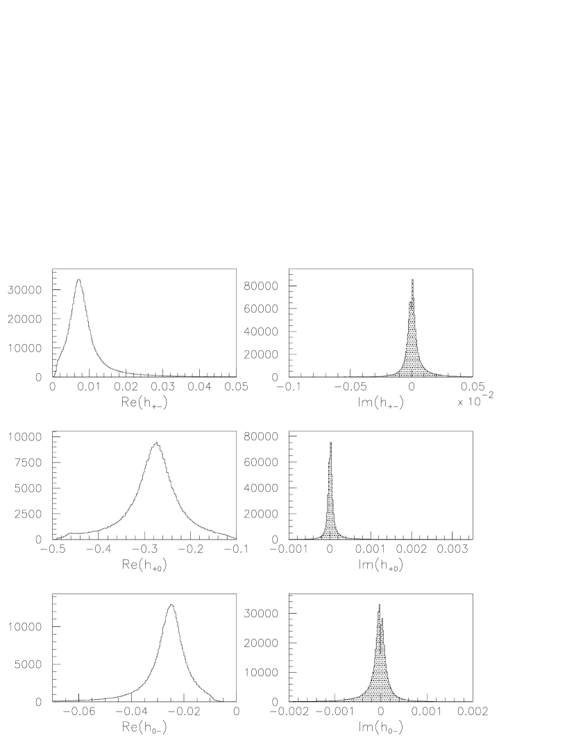
4) The non-diagonal matrix elements $h_{i,j}$ are mainly characterized by:

• The smallness of both their real and imaginary parts.

• ${\mathscr{I}\!m}/{\mathscr{R}\!e}\ \ \approx 0.001\to 0.1$.

• In the special case of $B^{+}\to\rho^{0}(\omega)\rho^{+},\ {\rm\mathscr{I}\!m{(h_{i,j})}}\ \approx 0.0$.

We arrive at the conclusion that there is a kind of universal behavior of the Density-Matrix Elements, whatever the decay $B\to{\pi}^{+}{\pi}^{-}V$ is ($V=\ K^{*0},K^{*{\pm}}\ ,\ {\rho}^{\pm}$).

Consequences for the angular distributions

In the helicity frame of each vector-meson, $V_{i}$, the angular distributions given above (see Eq. (8)) become simplified:

$\bullet$ According to the analytic expression for $g{(\phi)}$ and because of the small value of $\langle h_{+-}\rangle$, the azimuthal angle distribution is rather flat.

$\bullet$ From the expression of $f{({\cos}{\theta}_{1,2})}\$ and because of the dominant longitudinal part $h_{00}$, the polar angle distribution is $\approx{{\cos}^{2}}{\theta}$.

Branching ratios and asymmetries

$\star$ The energy $E_{i}$ and the momentum $p_{i}$ of each vector meson vary significantly according to the generated event. So, the branching ratio of each channel must be computed by Monte-Carlo methods from the fundamental relation:

$$d{\Gamma}(B\rightarrow V_{1}V_{2})\ =\ {\frac{1}{8{\pi}^{2}M}}\ {|{\cal M}(B\rightarrow V_{1}V_{2})|}^{2}\ {\frac{d^{3}{\vec{p}_{1}}}{2E_{1}}}\ {\frac{d^{3}{\vec{p}_{2}}}{2E_{2}}}\ {\delta}^{4}{(P-p_{1}-p_{2})}\ ,$$

and

$$Br{(B\rightarrow f)}=\frac{\Gamma{(B\rightarrow f)}}{\Gamma{(B\rightarrow All)}}\ .$$

$\star$ For a fixed value of ${q^{2}}/{{m_{b}}^{2}}$, the BRs depend strongly on the Form Factor model. They could vary up to a factor 2. $\star$ The relative difference between two conjugate branching ratios, $Br{(B\rightarrow f)}$ and $Br{({\bar{B}}\rightarrow{\bar{f}})}$, is almost independent of the form-factor models.

$\star$ An interesting effect is found in the variation of the differential asymmetry with respect to the $\pi\pi$ invariant mass which is defined by:

$$a_{CP}(m)=\frac{{\Gamma}_{m}{(B\rightarrow f)}-{\bar{\Gamma}}_{m}{(\bar{B}\rightarrow{\bar{f}})}}{{\Gamma}_{m}{(B\rightarrow f)}+{\bar{\Gamma}}_{m}{(\bar{B}\rightarrow{\bar{f}})}}\ .$$

$a_{CP}(m)$ is amplified in the vicinity of the $\omega$ resonance mass, a mass interval of $20\ {\rm MeV/}c^{2}$ around $M_{\omega}=\ 782{\rm MeV/}c^{2}$.

This differential asymmetry is $\approx 15\%$ in the case of $B^{0}\to K^{*0}{\rho}^{0}{(\omega)}\$ while it reaches $90\%$ in the channel $B^{\pm}\to{\rho}^{\pm}{\rho}^{0}{(\omega)}$. It is almost independent of the form-factor model and the only explanation of this surprising effect is the mixing of the two resonances ${\rho}^{0}\ {\rm and}\ {\omega}$ . These results have already been predicted analytically in the channel $B\to VP$ ($B\Rightarrow\rho^{0}(\omega){\pi},B\Rightarrow\rho^{0}(\omega)K$) by A.W. Thomas and his collaborators [9].

Some physical consequences can be deduced:

• A new method to detect and to measure the direct $CP$ Violation both in $B^{0}\ {\rm and}\ B^{\pm}$ decays can be exploited.

• According to the analytical expression:

$$a_{CP}^{dir}={\frac{A^{2}-{\bar{A}}^{2}}{A^{2}+{\bar{A}}^{2}}}=\frac{-2\ r\ {\sin{\delta}}\ {\sin{\phi}}}{1+r^{2}+2\ r\ {\cos{\delta}}\ {\cos{\phi}}}\ ,$$

an opportunity is offered for measuring $\sin{\Phi}$ , where $\Phi$ is a weak angle resulting from the CKM matrix elements:

$\star\ \Phi=Arg{[V_{tb}V^{*}_{ts}/V_{ub}V^{*}_{us}]}\ =\ {\gamma}$ in the case of $B\to{\rho}^{0}{(\omega)}K^{*}$,

$\star\ \Phi=Arg{[V_{tb}V^{*}_{td}/V_{ub}V^{*}_{ud}]}=\ {\beta}+{\gamma}\ ={\Pi}-{\alpha}$ in the case of $B\to{\rho}^{0}{(\omega)}{\rho}^{\pm}$.

$\bullet$ Another interesting result deduced from the above calculations is the ratio ${A^{P}}/{A^{T}}$ [10]. It depends on the free parameter ${q^{2}}/{{m_{b}}^{2}}$ and almost independent (except in the vicinity of the $\omega$ resonance mass) of the ${\pi}{\pi}$ invariant mass:

${{q^{2}}/{m_{b}^{2}}}=\ 0.3\ \Longrightarrow\ <r>\ =0.31\ {\pm}\ 0.03$ ,
${{q^{2}}/{m_{b}^{2}}}=\ 0.5\ \Longrightarrow\ <r>\ =0.27\ {\pm}\ 0.03$ ,

while the standard estimation of the ratio ${A^{P}}/{A^{T}}\ {\rm is}\approx\ 30\%$ (Buras et al).

5 Comparison with recent experimental results

The Belle and BaBar collaborations recently published their first results concerning the charmless $B$ decays into vector mesons, $B\to VV$ [8].

Belle Collaboration

Channel	Br($\times{10}^{-6}$)	$f_{L}={|H_{0}|}^{2}$
${\rho}^{0}{\rho}^{+}$	${31.7}\pm{7.1}(stat)^{+3.8}_{-6.7}(syst)$	$0.948\pm 0.106(stat)\pm 0.021(syst)$
Our results	$11.0\to 20.0$	$90\%$

Babar Collaboration

Channel	Br($\times{10}^{-6}$)	$f_{L}={|H_{0}|}^{2}$	$A_{CP}$
${\rho}^{0}K^{*+}$	${10.6}^{+3.0}_{-2.6}{\pm}2.4$	${0.96}^{+0.04}_{-0.15}{\pm}0.04$	${0.20}^{+0.32}_{-0.29}{\pm}0.04$
Our results	$2.3\to 5.8$	$87\%$	${-6.4\%}\to{-22\%}$
${\rho}^{0}{\rho}^{+}$	${22.5}^{+5.7}_{-5.4}{\pm}5.8$	${0.97}^{+0.03}_{-0.07}{\pm}0.04$	${-0.19}{\pm}0.23{\pm}0.03$
Our results	$11.0\to 20.0$	$90\%$	${-8.5\%}\to{-10\%}$

Because there is as yet insufficient data to allow one to bin data in the region of the $\omega$ resonance, one can only look at the global asymmetry $A_{CP}$ measured by BaBar. This is compatible with zero and the differential asymmetry with regard to ${\pi}{\pi}$ has not been investigated. We look forward with great anticipation to the time when the invariant mass distribution can be investigated.

6 Conclusion and perspectives

Monte-Carlo methods based on the helicity formalism have been used for all the numerical simulations of the channels $B\to{\pi}^{+}{\pi}^{-}V$ with $V=\ K^{*0},K^{*{\pm}},{\rho}^{\pm}$. Rigorous and detailed calculations of the $B$ decay density-matrix have been carried out completely and the corresponding code has been already implemented in the LHCb generator code.

$\bullet$ Despite the fact that the naive factorization hypothesis is very useful for weak hadronic $B$ decays, this method is limited because it involves theoretical uncertainties, some of them being very large.

However the physical consequences of this study are very interesting :

• The form factor model plays important role, especially in the estimation of the different branching ratios which can vary by up to a factor of 2.

• The longitudinal polarization is largely dominant, whatever the form factor model.

• The ${{\rho}^{0}}-{\omega}$ mixing is the main ingredient in the enhancement of direct $CP$ violation.

• A new way to look for $CP$ Violation is found and it can help to develop new methods for measuring the angles ${\gamma}\ {\rm and}\ {\alpha}$.

What remains to be done is to cross-check these predictions with experimental data coming from the LHC experiments.

Acknowledgments

One of us, Z.J.A., is very indebted to the organizers of this workshop, Dr Nick Brook and Dr Witek Pokorski from LHCb collaboration, for the opportunity they gave him to present the recent study on $B\to VV$ made in collaboration with theoretical colleagues at Adelaide University.

All of us enjoyed the exciting and illuminating discussions we got during the parallel sessions and regarding the broader aspects of $B$ physics.

Figure 1: Spectrum of $h_{--},h_{00},h_{++}$. Histograms on the left correspond to the channel $B^{0}\rightarrow\rho^{0}(\omega)K^{*0}$ where the parameters used are: ${q^{2}}/{{m^{2}}_{b}}=0.3$, $N_{c}^{eff}=2.84$, $\rho=0.229,\eta=0.325$ and form factors from the GH model. Histograms on the right correspond to the channel $B^{+}\rightarrow\rho^{0}(\omega)\rho^{+}$ for the same parameters with $N_{c}^{eff}=2.01$.

Figure 2: Spectrum of $\mathscr{R}\!e{(h_{ij})}\;{\rm and}\;\mathscr{I}\!m{(h_{ij})}$ where $i\neq j$. Histograms correspond to channel $B^{0}\rightarrow\rho^{0}(\omega)K^{*0}$ where the used parameters are: ${q^{2}}/{{m^{2}}_{b}}=0.3$, $N_{c}^{eff}=2.84$, $\rho=0.229,\eta=0.325$ and form factors from the GH model.

Figure 3: Spectrum of $\mathscr{R}\!e{(h_{ij})}\;{\rm and}\;\mathscr{I}\!m{(h_{ij})}$ where $i\neq j$. Histograms correspond to the channel $B^{+}\rightarrow\rho^{0}(\omega)\rho^{+}$ where the used parameters are: ${q^{2}}/{{m^{2}}_{b}}=0.3$, $N_{c}^{eff}=2.01$, $\rho=0.229,\eta=0.325$ and form factors from the GH model.

Figure 4: $CP$-violating asymmetry parameter $a_{CP}(m)$, as a function of the ${\pi}^{+}{\pi}^{-}$ invariant mass in the vicinity of the $\omega$ mass region for the channel $B^{0}\rightarrow\rho^{0}(\omega)K^{*0}$. Parameters are: ${q^{2}}/{{m^{2}}_{b}}=0.3$, $N_{c}^{eff}=2.84$, $\rho=0.229,\eta=0.325$. Solid triangles up and circles correspond to the BSW and GH form factor models respectively.

Figure 5: $CP$-violating asymmetry parameter $a_{CP}(m)$, as a function of the ${\pi}^{+}{\pi}^{-}$ invariant mass in the vicinity of the $\omega$ mass region for the channel $B^{+}\rightarrow\rho^{0}(\omega)\rho^{+}$. Parameters are: ${q^{2}}/{{m^{2}}_{b}}=0.3$, $N_{c}^{eff}=2.01$, $\rho=0.229,\eta=0.325$. Solid triangles down and circles correspond to the BSW and GH form factor models respectively.

References

- [1] I. Dunietz et al, Phys. Rev. D43 (1991) 2193.
- [2] M.E. Rose, ”Elementary theory of angular momentum”, Dover.
- [3] H. Quinn, ”Hadronic effects in two-body B decays”. Lectures at SLAC Summer Institute (1999).
- [4] A.J. Buras, Lect. Notes Phys. 558 (2000) 65, also in ‘Recent Developments in Quantum Field Theory’, Springer Verlag, edited by P. Breitenlohner, D. Maison and J. Wess (Springer-Verleg, Berlin, in press), hep-ph/9901409; R. Fleischer, Int. J. Mod. Phys. A12 (1997) 2459, Z. Phys. C62 (1994) 81, Z. Phys. C58 (1993) 483.
- [5] M. Bauer, B. Stech and M. Wirbel, Z. Phys. C34 (1987) 103; M. Wirbel, B. Stech and M. Bauer, Z. Phys. C29 (1985) 637.
- [6] Z.J. Ajaltouni et al, Eur.Phys.J. C 29, 215-233 (2003).
- [7] P. Langacker, Phys.Rev. D20, 2983 (1979).
- [8] B. Aubert et al (BaBar collaboration), ”Rates, Polarizations and asymmetries in Charmless Vector-Vector B Meson Decays”, hep-ex/0307026; J. Zhang et al (Belle collaboration), ”Observation of ” , hep-ex/0306007.
- [9] O. Leitner, X.-H. Guo and A.W. Thomas, Phys. Rev. D66 (2002) 096008, Phys. Rev. D63 (2001) 056012.
- [10] C. Rimbault, PhD thesis, report in progress, ”Etude de la violation directe de dans la désintegration du méson en deux mésons vecteurs non charmés. Analyse du canal dans le cadre de l’experience LHCb.”; O. Leitner, PhD Thesis, ”Direct violation in decays including mixing and covariant light-front dynamics”.