Exclusive Higgs Boson Production with bottom quarks at Hadron Colliders

Abstract

We present the next-to-leading order QCD corrected rate for the production of a scalar Higgs boson with a pair of high $p_{T}$ bottom and anti-bottom quarks at the Tevatron and at the Large Hadron Collider. Results are given for both the Standard Model and the Minimal Supersymmetric Standard Model. The exclusive $b\bar{b}h$ production rate is small in the Standard Model, but it can be greatly enhanced in the Minimal Supersymmetric Standard Model for large $\tan\beta$, making $b\bar{b}h$ an important discovery mode. We find that the next-to-leading order QCD results are much less sensitive to the renormalization and factorization scales than the lowest order results, but have a significant dependence on the choice of the renormalization scheme for the bottom quark Yukawa coupling.

I Introduction

One of the most important problems of particle physics is to uncover the origin of the electroweak symmetry breaking. In the simplest version of the Standard Model (SM) of particle physics, the breaking of the electroweak symmetry introduces a single physical scalar particle, the Higgs boson, that couples to both gauge bosons and fermions. Extensions of the Standard Model, like the Minimal Supersymmetric Standard Model (MSSM), introduce several scalar and pseudoscalar Higgs bosons. Finding experimental evidence for one or more Higgs particles is therefore a major goal of current and future accelerators. Direct searches at LEP2 require that the SM Higgs boson mass ($M_{h}$) be heavier than 114.4 GeV (at 95% c.l.) LEP Higgs Working Group (2003), while precision electroweak measurements imply $M_{h}\!<\!219$ GeV (at 95% c.l.) LEP Electroweak Working Group, talk presented by P. Wells . The light scalar Higgs particle of the MSSM ($h^{0}$) should have mass between the theoretical upper bound of about 130 GeV and the experimental lower bound from LEP2, $M_{h^{0}}\!>\!91$ GeV (at 95% c.l., $0.5\!<\tan\beta\!<\!2.4$ excluded) LEP Higgs Working Group (July 2001). In both cases, a Higgs boson should lie in a mass region which will certainly be explored at either the Fermilab $p\bar{p}$ Tevatron collider or at the CERN $pp$ Large Hadron Collider (LHC).

The dominant production mechanism for a SM Higgs boson in hadronic interactions is gluon fusion. Among the subleading modes, the associated production with either electroweak gauge bosons or top quark pairs, as well as weak boson fusion, play crucial roles. The inclusion of higher order QCD corrections is in general essential to stabilize the theoretical predictions of the corresponding rates. All of them have now been calculated at next-to-leading order (NLO) Han and Willenbrock (1991); Han et al. (1992); Dawson (1991); Djouadi et al. (1991); Graudenz et al. (1993); Spira et al. (1995); Beenakker et al. (2001); Reina and Dawson (2001); Beenakker et al. (2003); Reina et al. (2002); Dawson et al. (2003a, b) and, in the case of gluon fusion and associated production with gauge bosons, at next-to-next-to-leading order (NNLO) Harlander and Kilgore (2002); Anastasiou and Melnikov (2002); Harlander and Kilgore (2001); Catani et al. (2001); Ravindran et al. (2002); Brein et al. (2003) in perturbative QCD.

If the Standard Model is not the full story, however, then other mechanisms of Higgs production become very important. Here, we focus on Higgs boson production with a pair of bottom quark and antiquark. The coupling of the Higgs boson to a $b\bar{b}$ pair is suppressed in the Standard Model by the small factor, $m_{b}/v$, where $v\!=\!(\sqrt{2}G_{F})^{-1/2}\!=\!246$ GeV, implying that the SM Higgs production rate in association with bottom quarks is very small at both the Tevatron and the LHC. In a two Higgs doublet model or in the MSSM, however, this coupling grows with the ratio of neutral Higgs boson vacuum expectation values, $\tan\beta$, and can be significantly enhanced over the Standard Model coupling, leading to an observable production rate for a Higgs boson in association with bottom quarks in some regions of the parameter space.

The production of a Higgs boson in association with bottom quarks at hadron colliders has been the subject of much recent theoretical interest. At the tree level, the cross section is almost entirely dominated by $gg\to b\bar{b}h$, with only a small contribution from $q\bar{q}\to b\bar{b}h$, at both the Tevatron and the LHC. The integration over the phase space of the final state bottom quarks gives origin to large logarithms proportional to $\ln(m_{b}/\mu_{h})$ (where $\mu_{h}\!\simeq\!M_{h}$), which arise from the splitting of an initial gluon into a pair of almost on-shell collinear bottom quarks. The use of bottom quark parton distribution functions in the proton (or anti-proton) sums these large logarithms to all orders, and could therefore improve a fixed order calculation. The inclusive cross section for $b\bar{b}h$ production should then be dominated by the bottom quark fusion process $b\bar{b}\to h$, as originally proposed in Ref. Dicus and Willenbrock (1989). Some important progress has been achieved recently. The $b\bar{b}\to h$ production process has been calculated at NNLO in QCD Harlander and Kilgore (2003). At NLO Dicus et al. (1999); Balazs et al. (1999a), the residual factorization scale dependence is quite large, but at NNLO there is almost no scale dependence. Interestingly enough the NNLO results show that the perturbative cross section is better behaved when the factorization scale is $\mu_{f}\!\simeq\!M_{h}/4$ (and the renormalization scale is $\mu_{r}\!\simeq\!M_{h}$), as expected on quite general theoretical grounds Rainwater et al. (2002); Plehn (2003); Maltoni et al. (2003); Boos and Plehn (2003). Moreover, the inclusive $b\bar{b}h$ cross section has been obtained at NLO in QCD via a fixed order calculation that includes the $O(\alpha_{s})$ corrections to the parton level processes $gg,q\bar{q}\to b\bar{b}h$ Talk presented by M. Krämer ; Talk presented by M. Spira ; Dittmaier et al. (2003). The obtained results are compatible with $b\bar{b}\to h$ at NNLO, and show that there is actually no large discrepancy between the NLO fixed order calculation and the use of $b$-quark parton distribution functions, contrary to what was originally claimed. However, the results of the fixed order calculation have a substantial scale dependence and a better control of the residual large uncertainty is desirable for a complete understanding of the comparison between the two approaches.

In spite of its theoretical interest, the inclusive cross section is experimentally relevant only if a Higgs boson can be detected above the background without tagging any of the outgoing bottom quarks. Higgs production from $b\bar{b}$ fusion could be useful, for instance, in a supersymmetric model with a large value of $\tan\beta$, when combined with the decays $h^{0},H^{0}\to\mu^{+}\mu^{-}$ and $h^{0},H^{0}\to\tau^{+}\tau^{-}$ CMS Collaboration (1994); Barger and Kao (1998); Richter-Was et al. (1998); ATLAS Collaboration (1999). However, even in this case, the inclusive measurement of a Higgs signal would not determine the bottom quark Yukawa coupling unambiguously, since it should be interpreted as the result of the combined action of other production channels besides $b\bar{b}\to h^{0},H^{0}$ (e.g. $gg\to h^{0},H^{0}$).

Requiring one or two high $p_{T}$ bottom quarks in the final state reduces the signal cross section with respect to $b\bar{b}\to h$, but it also greatly reduces the background Carena et al. (1999); ATLAS Collaboration (1999). Moreover, it assures that the detected Higgs boson has been radiated off a bottom or anti-bottom quark and the corresponding cross section is therefore unambiguously proportional to the bottom quark Yukawa coupling. Using arguments similar to the ones illustrated above for the case of the inclusive cross section, one can argue that if the final state has one high $p_{T}$ bottom quark then the relevant subprocess is $gb\to bh$ Dicus et al. (1999). The cross section for $gb\to bh$ has been computed including NLO QCD corrections Campbell et al. (2003) and the residual uncertainty due to higher order QCD corrections is small. On the other hand, if the final state has two high $p_{T}$ bottom quarks and a Higgs boson, then no final state bottom quark can originate from a bottom quark parton distribution function. The lowest order relevant parton level processes are unambiguously $gg\to b\bar{b}h$ and $q\bar{q}\to b\bar{b}h$. While the rate for this final state is considerably smaller than for the $b\bar{b}\to h$ and $gb\to bh$ subprocesses, the background is correspondingly reduced. The final states can be further categorized according to the decay of the Higgs boson. Existing studies have considered mostly the dominant Higgs decay channel, $h\to b\bar{b}$ Dai et al. (1995, 1996); Carena et al. (1999); Affolder et al. (2001); Carena et al. (2000); Balazs et al. (1999b); ATLAS Collaboration (1999); Richter-Was and Froidevaux (1997), but also $h\to\tau^{+}\tau^{-}$ Carena et al. (1999) and $h\to\mu^{+}\mu^{-}$ Dawson et al. (2002); Boos et al. (2003).

In this paper, we present the NLO QCD corrected rates and phase space distributions for the fully exclusive processes $pp,p\bar{p}\to b\bar{b}h$, where the final state includes two high $p_{T}$ bottom quarks. In order to reproduce as closely as possible the currently used experimental cuts, we require the final state bottom quark/anti-quark to have a transverse momentum higher than $p_{T}^{cut}\!=\!20$ GeV and a pseudorapidity $|\eta|\!\leq\!2$ for the Tevatron and $|\eta|\!\leq\!2.5$ for the LHC. The cut on $p_{T}^{b,\bar{b}}$ greatly affects the cross section and we therefore study the dependence of the cross section on this cut. Similar results have been recently presented in Ref. Dittmaier et al. (2003), where however no cut on the pseudorapidity has been imposed. Our discussion will focus on assessing the uncertainty of the theoretical prediction for the exclusive $pp,p\bar{p}\to b\bar{b}h$ rates, after the full set of NLO QCD corrections has been included. We will show how the large dependence on the unphysical renormalization and factorization scales present in the lowest order (LO) calculation of the cross section is greatly reduced at NLO. Moreover, we will study the dependence on the choice of renormalization scheme for the bottom quark Yukawa coupling. While for Higgs decays and Higgs production in $e^{+}e^{-}$ collisions using the $\overline{MS}$ definition of the bottom quark Yukawa coupling is an efficient way of improving the perturbative calculation of the corresponding rate by resumming large logarithms at all orders Braaten and Leveille (1980); Drees and Hikasa (1990); Gorishnii et al. (1984); Kataev and Kim (1994), this may be less compelling in the case of hadronic Higgs production. Finally, we will extend our calculation to the scalar sector of the MSSM, including the SM QCD corrections at NLO. Preliminary results of the study described in this paper have been already presented at several conferences Talks presented by L. Reina .

The plan of the paper is as follows. In Section II we present an overview of our calculation. Since the NLO QCD corrections to $q\bar{q},gg\to b\bar{b}h$ proceed in strict analogy to those for $q\bar{q}\to t\bar{t}h$ Beenakker et al. (2001); Reina and Dawson (2001); Reina et al. (2002); Beenakker et al. (2003) and $gg\to t\bar{t}h$ Beenakker et al. (2001, 2003); Dawson et al. (2003a, b), we will be very brief on details and devote more time to the discussion of the residual theoretical uncertainty, emphasizing those aspects that are characteristic of the $b\bar{b}h$ production process. Numerical results for the Tevatron and the LHC will be presented in Section III, for both the SM Higgs boson and the scalar MSSM Higgs bosons in some prototype regions of the model parameter space. Section IV contains our conclusions.

II Calculation

II.1 Basics

The total cross section for $pp,p\bar{p}\to b\bar{b}h$ at ${\cal O}(\alpha_{s}^{3})$ can be written as:

$$\sigma_{\scriptscriptstyle NLO}(pp,p\bar{p}\to b\bar{b}h)=$$

$$\sum_{ij}\frac{1}{1+\delta_{ij}}\int dx_{1}dx_{2}\left[{\cal F}_{i}^{p}(x_{1},\mu){\cal F}_{j}^{p,\bar{p}}(x_{2},\mu){\hat{\sigma}}^{ij}_{\scriptscriptstyle NLO}(x_{1},x_{2},\mu)+(1\leftrightarrow 2)\right]\,\,\,,$$ (1)

where ${\cal F}_{i}^{p,\bar{p}}$ are the NLO parton distribution functions (PDFs) for parton $i$ in a proton or anti-proton, defined at a generic factorization scale $\mu_{f}\!=\!\mu$, and ${\hat{\sigma}}^{ij}_{\scriptscriptstyle NLO}$ is the ${\cal O}(\alpha_{s}^{3})$ parton-level total cross section for incoming partons $i$ and $j$, made of the channels $q\bar{q},gg\to b\bar{b}h$ and $(q,\bar{q})g\to b\bar{b}h(q,\bar{q})$, and renormalized at an arbitrary scale $\mu_{r}$ which we also take to be $\mu_{r}\!=\!\mu$. Throughout this paper we will always assume the factorization and renormalization scales to be equal, $\mu_{r}\!=\!\mu_{f}\!=\!\mu$. The partonic center-of-mass energy squared, $s$, is given in terms of the hadronic center-of-mass energy squared, $s_{\scriptscriptstyle H}$, by $s=x_{1}x_{2}s_{\scriptscriptstyle H}$. At both the Tevatron and the LHC, the dominant contribution is from the gluon-gluon initial state, although we include all initial states.

The NLO parton-level total cross section reads

$${\hat{\sigma}}_{\scriptscriptstyle NLO}^{ij}(x_{1},x_{2},\mu)={\hat{\sigma}}_{\scriptscriptstyle LO}^{ij}(x_{1},x_{2},\mu)+\delta{\hat{\sigma}}_{\scriptscriptstyle NLO}^{ij}(x_{1},x_{2},\mu)\,\,\,,$$ (2)

where ${\hat{\sigma}}_{\scriptscriptstyle LO}^{ij}(x_{1},x_{2},\mu)$ is the ${\cal O}(\alpha_{s}^{2})$ Born cross section, and $\delta{\hat{\sigma}}_{\scriptscriptstyle NLO}^{ij}(x_{1},x_{2},\mu)$ consists of the ${\cal O}(\alpha_{s})$ corrections to the Born cross sections for $gg,q\bar{q}\to b\bar{b}h$ and of the tree level $(q,\bar{q})g\to b\bar{b}h(q,\bar{q})$ processes, including the effects of mass factorization.

The evaluation of ${\hat{\sigma}}^{ij}_{\scriptscriptstyle NLO}$ proceeds along the same lines as the corresponding calculation for $t\bar{t}h$ production Beenakker et al. (2001); Reina and Dawson (2001); Beenakker et al. (2003); Reina et al. (2002); Dawson et al. (2003a, b) and we refer to Refs. Reina et al. (2002); Dawson et al. (2003b) for a detailed description of the techniques used in our calculation. We notice that, in view of the generalization to the MSSM with a very enhanced bottom quark Yukawa coupling, both top and bottom quark loops need to be considered in those virtual diagrams where the Higgs boson couples directly to a closed loop of fermions, a sample of which is illustrated in Fig. 1.

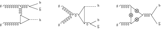
Figure 1: Sample of diagrams corresponding to ${\cal O}(\alpha_{s})$ virtual corrections where the Higgs boson couples to an internal fermion loop and not to the external $b\bar{b}$ pair. The circled cross denotes all possible insertion of the final state Higgs boson leg, each insertion corresponding to a different diagram.

Contrary to the case of $t\bar{t}h$ production, the NLO cross section for $b\bar{b}h$ production depends significantly on the renormalization scheme used for the bottom quark Yukawa coupling, i.e. for the bottom quark mass appearing in $g_{b\bar{b}h}\!=\!m_{b}/v$. In our calculation of the NLO $p\bar{p},pp\to b\bar{b}h$ cross section we have considered, for the renormalization of the bottom quark Yukawa coupling, both the on-shell and the $\overline{MS}$ subtraction schemes (in the $t\bar{t}h$ case we only used the on-shell top quark renormalized mass everywhere Dawson et al. (2003b)). The $\overline{MS}$ scheme results in a running bottom quark Yukawa coupling and potentially gives better control over higher order contributions beyond the 1-loop corrections. We will study the origin and magnitude of the residual scheme dependence in Sections II.2 and III.1.

II.2 Renormalization scheme dependence

The ultraviolet (UV) divergences arising from self-energy and vertex ${\cal O}(\alpha_{s})$ virtual corrections to $q\bar{q},gg\to b\bar{b}h$ are regularized in $d\!=4-2\epsilon$ dimensions and renormalized by introducing counterterms for the wave functions of the external fields ($\delta Z_{2}^{(q)}$ (for $q\!=\!u,d,c,s$), $\delta Z_{2}^{(b)}$ for the bottom quark, and $\delta Z_{3}$ for the gluon), for the bottom quark mass, $\delta m_{b}$, and for the bottom quark Yukawa and strong coupling constants, $\delta g_{b\bar{b}h}$ and $\delta Z_{\alpha_{s}}$. We follow the same renormalization prescription and notation adopted in Refs. Reina et al. (2002); Dawson et al. (2003b) for the NLO $t\bar{t}h$ inclusive cross section. Consequently, we fix the wave-function renormalization constants of the external massless quark fields, $\delta Z_{2}^{(q)}$, using on-shell subtraction, while we define the wave function renormalization constant of external gluons, $\delta Z_{3}$, using the $\overline{MS}$ subtraction scheme and the $\alpha_{s}$ renormalization constant, $\delta Z_{\alpha_{s}}$, using the $\overline{MS}$ scheme modified to decouple the top quark Collins et al. (1978); Nason et al. (1989). Explicit expressions for $\delta Z_{2}^{(q)}$, $\delta Z_{3}$, and $\delta Z_{\alpha_{s}}$ can be found in Refs. Reina et al. (2002); Dawson et al. (2003b).

However, given the large sensitivity of the $\overline{MS}$ bottom quark mass to the renormalization scale and given the prominent role it plays in the $b\bar{b}h$ production cross section through the overall bottom quark Yukawa coupling, we investigate here the dependence of the final results on the renormalization prescription adopted for the bottom quark. We consider both the on-shell ($OS$) and $\overline{MS}$ subtraction schemes, for both the bottom quark mass and wave function renormalization constants.

When using the $OS$ subtraction scheme, we fix the wave function renormalization constant of the external bottom quark field, $(\delta Z_{2}^{(b)})_{OS}$, and the mass renormalization constant, $(\delta m_{b})_{OS}$, by requiring that

$$\hat{\Sigma}_{b}(\not{p}=m_{b})=0\;\;\;;\;\;\;\lim_{\not{p}\to m_{b}}\frac{\hat{\Sigma}_{b}(\not{p})}{\not{p}-m_{b}}=0\,\,\,,$$ (3)

where

$$\hat{\Sigma}_{b}=(\not{p}-m_{b})\left(\Sigma_{V}+\delta Z_{2}^{(b)}\right)+m_{b}\left(\Sigma_{S}+\Sigma_{V}-\frac{\delta m_{b}}{m_{b}}\right)$$ (4)

denotes the renormalized bottom quark self-energy at 1-loop in QCD, expressed in terms of the vector, $\Sigma_{V}$, and scalar, $\Sigma_{S}$, parts of the unrenormalized self-energy, and of the mass and wave function renormalization constants. Using Eq. (3) in $d\!=\!4-2\epsilon$ dimensions one finds

$$\left(\delta Z_{2}^{(b)}\right)_{OS} = -\frac{\alpha_{s}}{4\pi}\,C_{F}\left(\frac{4\pi\mu^{2}}{m_{b}^{2}}\right)^{\epsilon}\Gamma(1+\epsilon)\left(\frac{1}{\epsilon_{\scriptscriptstyle UV}}+4+\frac{2}{\epsilon_{\scriptscriptstyle IR}}\right)\,\,\,,$$ (5)

$$\left(\frac{\delta m_{b}}{m_{b}}\right)_{OS} = -\frac{\alpha_{s}}{4\pi}\,C_{F}\left(\frac{4\pi\mu^{2}}{m_{b}^{2}}\right)^{\epsilon}\Gamma(1+\epsilon)\left(\frac{3}{\epsilon_{\scriptscriptstyle UV}}+4\right)\,\,\,,$$ (6)

where we have explicitly distinguished between ultraviolet and infrared divergences. The infrared divergences are cancelled between virtual and real soft and collinear contributions according to the pattern outlined in Refs. Reina et al. (2002); Dawson et al. (2003b), to which we refer for more details.

In the $\overline{MS}$ scheme, the bottom quark renormalization constants are fixed by requiring that they cancel the UV divergent parts of the bottom quark self energy $\hat{\Sigma}_{b}$ of Eq. (4), i.e.

$$\left(\delta Z_{2}^{(b)}\right)_{\overline{MS}} = -\frac{\alpha_{s}}{4\pi}\,C_{F}\left(4\pi\right)^{\epsilon}\Gamma(1+\epsilon)\frac{1}{\epsilon_{\scriptscriptstyle UV}}\,\,\,,$$ (7)

$$\left(\frac{\delta m_{b}}{m_{b}}\right)_{\overline{MS}} = -\frac{\alpha_{s}}{4\pi}\,C_{F}\left(4\pi\right)^{\epsilon}\Gamma(1+\epsilon)\frac{3}{\epsilon_{\scriptscriptstyle UV}}\,\,\,.$$ (8)

According to the LSZ prescription Lehmann et al. (1955), one also needs to consider the insertion of the renormalized one-loop self-energy corrections on the external bottom quark legs. While these terms are zero in the $OS$ scheme (see Eq. (3)), they are not zero in the $\overline{MS}$ scheme. Together with $(\delta Z_{2}^{(b)})_{\overline{MS}}$, their contribution to the NLO cross section equals the contribution of the wave function counterterm in the $OS$ scheme, $(\delta Z_{2}^{(b)})_{OS}$, as expected from the LSZ prescription itself. The cross section does not depend on the renormalization of the external particle wave functions.

We therefore focus on the scheme dependence induced by the choice of different subtraction schemes for the bottom quark mass. We note that the bottom quark mass counterterm has to be used twice: once to renormalize the bottom quark mass appearing in internal propagators and once to renormalize the bottom quark Yukawa coupling. Indeed, if one considers only QCD corrections, the counterterm for the bottom quark Yukawa coupling,

$$\delta g_{b\bar{b}h}\!=\!\frac{\delta m_{b}}{v}\,\,\,,$$ (9)

coincides with the counterterm for the bottom quark mass, since the SM Higgs vacuum expectation value $v$ is not renormalized at 1-loop in QCD. This stays true when we generalize the $g_{b\bar{b}h}$ coupling from the SM to the case of the scalar Higgs bosons of the MSSM.

At 1-loop order in QCD, the relation between the pole mass, $m_{b}$, and the $\overline{MS}$ mass, $\overline{m}_{b}(\mu)$, is indeed determined by the difference between the $OS$ and $\overline{MS}$ bottom mass counterterms, $\frac{\displaystyle{\alpha_{s}}}{\displaystyle{4\pi}}\delta CT$, since

$$\overline{m}_{b}(\mu)=m_{b}\left\{1-\frac{\alpha_{s}(\mu)}{4\pi}C_{F}\left[3\ln\left(\frac{\mu^{2}}{m_{b}^{2}}\right)+4\right]\right\}\equiv m_{b}\left[1-\frac{\alpha_{s}(\mu)}{4\pi}\delta CT(\mu)\right]\,\,\,.$$ (10)

Adopting the $OS$ or $\overline{MS}$ prescription consists of using either Eq. (6) or Eq. (8) for the bottom mass counterterms while substituting $m_{b}$ or $\overline{m}_{b}(\mu)$ respectively in both the bottom quark propagator and Yukawa coupling. At ${\cal O}(\alpha_{s}^{3})$ the two prescriptions give identical results. Indeed, replacing $m_{b}$ by $\overline{m}_{b}(\mu)$ in the Yukawa coupling adds a term

$$-\frac{\alpha_{s}(\mu)}{2\pi}\delta CT(\mu)\hat{\sigma}_{\scriptscriptstyle LO}+{\cal O}(\alpha_{s}^{4})$$ (11)

to the NLO parton level cross section, which compensates exactly for the difference in the OS and $\overline{MS}$ counterterms. On the other hand, using the $\overline{MS}$ mass in the bottom quark propagator,

$$\frac{i}{\not{p}-\overline{m}_{b}(\mu)}=\frac{i}{\not{p}-m_{b}}\left[1+im_{b}\frac{\alpha_{s}}{4\pi}\delta CT(\mu)\frac{i}{\not{p}-m_{b}}\right]+{\cal O}(\alpha_{s}^{2})\,\,\,,$$ (12)

of the LO cross section leads to an extra contribution to the $\overline{MS}$ NLO cross section which, together with the $\overline{MS}$ mass counterterm insertions into the internal bottom quark propagators (see diagrams $S_{1}$ in Fig. 2 of Ref. Reina et al. (2002) and $S_{2}$, $S_{3}$, and $S_{4}$ in Fig. 2 of Ref. Dawson et al. (2003b)), coincides with the corresponding mass counterterm insertions in the $OS$ scheme at ${\cal O}(\alpha_{s}^{3})$.

Therefore, using OS or $\overline{MS}$ at ${\cal O}(\alpha_{s}^{3})$ is perturbatively consistent, the difference between the two schemes being of higher order and hence, strictly speaking, part of the theoretical uncertainty of the NLO calculation. One notices however that some of the large logarithms involved in the renormalization procedure of the NLO cross section come from the renormalization of the bottom quark mass, and are nicely factored out by using the $\overline{MS}$ bottom mass in the bottom quark Yukawa coupling (see Eq. (10)). Therefore one should consider reorganizing the perturbative expansion in terms of leading logarithms (of the form $\alpha_{s}^{n}(\mu)\ln^{n}(\mu^{2}/m_{b}^{2})$) or next-to-leading-logarithms (of the form $\alpha_{s}^{n}(\mu)\ln^{n-1}(\mu^{2}/m_{b}^{2})$, for $\mu\!\simeq\!M_{h}$), as obtained by replacing the $\overline{MS}$ bottom mass in the Yukawa coupling by the corresponding 1-loop or 2-loop renormalization group improved $\overline{MS}$ masses:

$$\overline{m}_{b}(\mu)_{1l} = m_{b}\left[\frac{\alpha_{s}(\mu)}{\alpha_{s}(m_{b})}\right]^{c_{0}/b_{0}}\,\,\,,$$ (13)

$$\overline{m}_{b}(\mu)_{2l} = m_{b}\left[\frac{\alpha_{s}(\mu)}{\alpha_{s}(m_{b})}\right]^{c_{0}/b_{0}}\left[1+\frac{c_{0}}{b_{0}}\left(c_{1}-b_{1}\right)\frac{\alpha_{s}(\mu)-\alpha_{s}(m_{b})}{\pi}\right]\left(1-\frac{4}{3}\frac{\alpha_{s}(m_{b})}{\pi}\right)\,\,\,,$$

where

$$b_{0} = \frac{1}{4\pi}\left(\frac{11}{3}N-\frac{2}{3}n_{lf}\right)\,\,\,,\,\,\,c_{0}=\frac{1}{\pi}\,\,\,,$$ (15)

$$b_{1} = \frac{1}{2\pi}\frac{51N-19n_{lf}}{11N-2n_{lf}}\,\,\,,\,\,\,c_{1}=\frac{1}{72\pi}\left(101N-10n_{lf}\right)\,\,\,,$$ (16)

are the one and two loop coefficients of the QCD $\beta$-function and mass anomalous dimension $\gamma_{m}$, while $N\!=\!3$ is the number of colors and $n_{lf}\!=\!5$ is the number of light flavors.

In both Higgs boson decays to heavy quarks and Higgs boson production with heavy quarks in $e^{+}e^{-}$ collisions, using Eq. (13) at LO and Eq. (II.2) at NLO in the Yukawa coupling proves to be a very powerful way to stabilize the perturbative calculation of the cross section Braaten and Leveille (1980). The difference between LO and NLO rates is reduced and the dependence on the renormalization and factorization scales at NLO is very mild, indicating a very small residual theoretical error or equivalently a very good convergence of the perturbative expansion of the corresponding rate. This is due to the fact that in these cases to a large extent the ${\cal O}(\alpha_{s})$ QCD corrections amount to a renormalization of the heavy quark mass in the Yukawa coupling. In more complicated cases, like the case of the hadronic cross section discussed in this paper, the previous argument is not automatically true.

Using the $OS$ or $\overline{MS}$ bottom quark mass mainly affects the Yukawa coupling. Therefore, in the hadronic case, we will look at the different behavior of the NLO cross section when the bottom quark Yukawa coupling is renormalized either in the $OS$ or in the $\overline{MS}$ scheme, keeping the bottom quark pole mass everywhere else. Fig. 2 of Section III shows the renormalization and factorization scale dependence of the LO and NLO cross sections for $pp,p\bar{p}\to b\bar{b}h$ obtained using in the Yukawa coupling either the pole mass $m_{b}$ or the $\overline{MS}$ running mass $\overline{m}_{b}(\mu)$ in Eq. (13) (at LO) and (II.2) (at NLO). The use of $\overline{m}_{b}(\mu)$ both at LO and NLO seems to improve the perturbative calculation of the cross section, since the NLO $\overline{MS}$ cross section is better behaved than the NLO $OS$ cross section at low scales and since the difference between LO and NLO cross section is smaller when the bottom quark Yukawa coupling is renormalized in the $\overline{MS}$ scheme than in the $OS$ scheme. However, both the OS and the $\overline{MS}$ cross sections have very well defined regions of minimum sensitivity to the variation of the renormalization/factorization scale and these regions do not quite overlap. The difference between the $OS$ and $\overline{MS}$ results at the plateau should rather be interpreted, in the absence of a NNLO calculation, as an upper bound on the theoretical uncertainty.

The origin of the large difference between the $OS$ and $\overline{MS}$ NLO cross sections illustrated in Fig. 2 can be understood by studying the numerical effect of the higher order terms that are included in the NLO $\overline{MS}$ cross section when $\overline{m}_{b}(\mu)$ is used in the Yukawa coupling. The parton level NLO cross sections for $ij\to b\bar{b}h$ ($ij\!=\!q\bar{q},gg$) in the $OS$ and $\overline{MS}$ prescription explained above can be written as:

$${\hat{\sigma}}^{ij}_{\scriptscriptstyle NLO,OS}(x_{1},x_{2},\mu) = m_{b}^{2}\alpha_{s}^{2}(\mu)\left\{\phantom{\frac{1}{2}}\,g^{ij}_{\scriptscriptstyle LO}(x_{1},x_{2})\right.$$

$$+ \left.\frac{\alpha_{s}(\mu)}{4\pi}\left[g^{ij}_{\scriptscriptstyle NLO}(x_{1},x_{2},\mu)-2g^{ij}_{\scriptscriptstyle LO}(x_{1},x_{2})\delta CT(\mu)+\frac{m_{t}}{m_{b}}g^{ij}_{\scriptscriptstyle cl}(x_{1},x_{2})\right]\right\}\,\,\,,$$

$${\hat{\sigma}}^{ij}_{\scriptscriptstyle NLO,\overline{MS}}(x_{1},x_{2},\mu) = \overline{m}_{b}^{2}(\mu)\alpha_{s}^{2}(\mu)\left\{\phantom{\frac{1}{2}}\,g^{ij}_{\scriptscriptstyle LO}(x_{1},x_{2})\right.$$ (18)

$$+ \left.\frac{\alpha_{s}(\mu)}{4\pi}\left[g^{ij}_{\scriptscriptstyle NLO}(x_{1},x_{2},\mu)+\frac{m_{t}}{\overline{m}_{b}(\mu)}g^{ij}_{\scriptscriptstyle cl}(x_{1},x_{2})\right]\right\}\,\,\,,$$

where the dependence on the renormalization scale is explicitly given. $\alpha_{s}(\mu)$ is the 2-loop strong coupling, $m_{b}$ is the bottom pole mass, and $\overline{m}_{b}(\mu)$ is the bottom quark $\overline{MS}$ mass. $g^{ij}_{\scriptscriptstyle LO}$, $g^{ij}_{\scriptscriptstyle NLO}$ and $g_{\scriptscriptstyle cl}^{ij}$ have been defined in such a way that they are the same in the $OS$ and the $\overline{MS}$ schemes. They correspond respectively to the ${\cal O}(\alpha_{s}^{2})$ ($g^{ij}_{\scriptscriptstyle LO}$) and ${\cal O}(\alpha_{s}^{3})$ ($g^{ij}_{\scriptscriptstyle NLO}$) contributions to the NLO QCD cross section, from which we have singled out the ${\cal O}(\alpha_{s})$ virtual corrections where the Higgs boson couples to a top quark in a closed fermion loop ($g^{ij}_{cl}$, see, e.g., diagrams in Fig. 1) as well as $\delta CT(\mu)$, i.e. the difference between the $OS$ and $\overline{MS}$ bottom mass counterterms defined in Eq. (10). Using Eqs. (II.2) and (18), one can easily verify that the difference between the parton level NLO cross sections obtained by using either the $OS$ or the $\overline{MS}$ scheme for the bottom quark Yukawa coupling is, as expected, of higher order in $\alpha_{s}$, i.e.:

$$\hat{\Delta} = {\hat{\sigma}}^{ij}_{\scriptscriptstyle NLO,OS}-{\hat{\sigma}}^{ij}_{\scriptscriptstyle NLO,\overline{MS}}$$ (19)

$$= \alpha_{s}^{2}(\mu)g^{ij}_{\scriptscriptstyle LO}(x_{1},x_{2})\left[m_{b}^{2}-\overline{m}_{b}^{2}(\mu)-m_{b}^{2}\frac{\alpha_{s}(\mu)}{2\pi}\delta CT(\mu)\right]$$

$$+ \frac{\alpha_{s}^{3}(\mu)}{4\pi}(m_{b}^{2}-\overline{m}_{b}^{2}(\mu))\left[g^{ij}_{\scriptscriptstyle NLO}(x_{1},x_{2},\mu)+\frac{m_{t}}{m_{b}+\overline{m}_{b}(\mu)}g^{ij}_{\scriptscriptstyle cl}(x_{1},x_{2})\right]\,\,\,.$$

The term in the first bracket of Eq. (19) vanishes at ${\cal O}(\alpha_{s}^{3})$, as can be easily verified by using Eq. (10). Hence all the terms in Eq. (19) only contribute at $O(\alpha_{s}^{4})$ and higher. However, while the first term is in general quite small, the term proportional to $g_{\scriptscriptstyle NLO}^{ij}(x_{1},x_{2},\mu)$ can be large and has a non trivial scale dependence that we can formally write as:

$$g_{\scriptscriptstyle NLO}^{ij}(x_{1},x_{2},\mu)=g_{1}^{ij}(x_{1},x_{2})+\tilde{g}_{1}^{ij}(x_{1},x_{2})\ln\left(\frac{\mu^{2}}{s}\right)\,\,\,.$$ (20)

From renormalization group arguments Reina et al. (2002); Dawson et al. (2003b) one can see that $\tilde{g}_{1}^{ij}(x_{1},x_{2})$ is given by:

$$\tilde{g}_{1}^{ij}(x_{1},x_{2}) = 2\,\left\{(4\pi b_{0}+4)g^{ij}_{\scriptscriptstyle LO}(x_{1},x_{2})-\sum_{k}\left[\int_{\rho}^{1}dz_{1}P_{ik}(z_{1})g^{kj}_{\scriptscriptstyle LO}(x_{1}z_{1},x_{2})\right.\right.$$ (21)

$$+ \left.\left.\int_{\rho}^{1}dz_{2}P_{jk}(z_{2})g^{ik}_{\scriptscriptstyle LO}(x_{1},x_{2}z_{2})\right]\right\}\,\,\,,$$

where $\rho\!=\!(2m_{b}+M_{h})^{2}/s$, $P_{ij}(z)$ denotes the lowest-order regulated Altarelli-Parisi splitting function Altarelli and Parisi (1977) of parton $i$ into parton $j$, when $j$ carries a fraction $z$ of the momentum of parton $i$, (see e.g. Section V of Ref. Dawson et al. (2003b)), and $b_{0}$ is given in Eq. (15). As a result, $\hat{\Delta}$, defined in Eq. (19), turns out to have a non trivial scale dependence and, thus, the difference between the NLO hadronic cross section calculated with the $OS$ or with the $\overline{MS}$ definition of the bottom quark Yukawa coupling can be numerically quite significant for some values of the renormalization/factorization scale, as we will illustrate in Section III (see Figs. 2 and 3).

III Numerical results

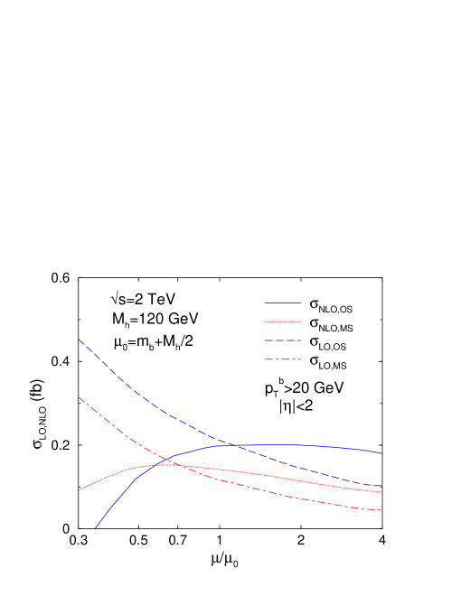
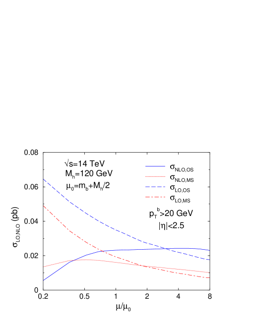
Figure 2: $\sigma_{\scriptscriptstyle NLO}$ and $\sigma_{\scriptscriptstyle LO}$ for $p\bar{p}\to b\bar{b}h$ at $\sqrt{s}\!=\!2$ TeV (top) and for $pp\to b\bar{b}h$ at $\sqrt{s}\!=\!14$ TeV (bottom) as a function of the renormalization/factorization scale $\mu$, for $M_{h}=120$ GeV. The curves labeled $\sigma_{\scriptscriptstyle LO,OS}$ and $\sigma_{\scriptscriptstyle NLO,OS}$ use the $OS$ renormalization scheme for the bottom quark Yukawa coupling, while the curves labeled $\sigma_{\scriptscriptstyle LO,MS}$ and $\sigma_{\scriptscriptstyle NLO,MS}$ use the $\overline{MS}$ scheme.

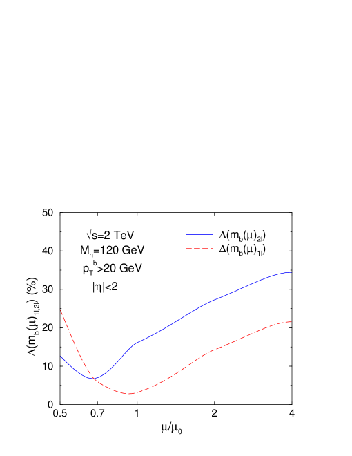
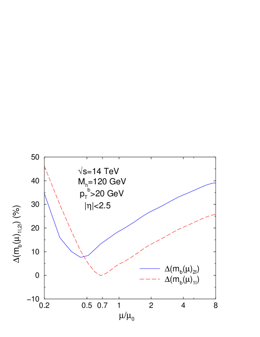
Figure 3: The absolute value of the percentage difference $\Delta(\%)\!=\!(\sigma_{\scriptscriptstyle NLO,OS}-\sigma_{\scriptscriptstyle NLO,\overline{MS}})/(\sigma_{\scriptscriptstyle NLO,OS}+\sigma_{\scriptscriptstyle NLO,\overline{MS}})$ for $p\bar{p}\to b\bar{b}h$ at $\sqrt{s}=2$ TeV (top) and for $pp\to b\bar{b}h$ at $\sqrt{s}=14$ TeV (bottom) as a function of the renormalization/factorization scale $\mu$, for $M_{h}=120$ GeV. The $OS$ and $\overline{MS}$ labels refer to the renormalization scheme chosen for the bottom quark Yukawa coupling. The curves labeled as $\Delta(m_{b}(\mu)_{1l})$ and $\Delta(m_{b}(\mu)_{2l})$ use the $\overline{MS}$ bottom quark Yukawa coupling with the 1-loop running mass of Eq. (13) and the 2-loop running mass of Eq. (II.2), respectively.

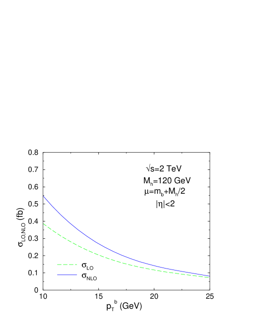
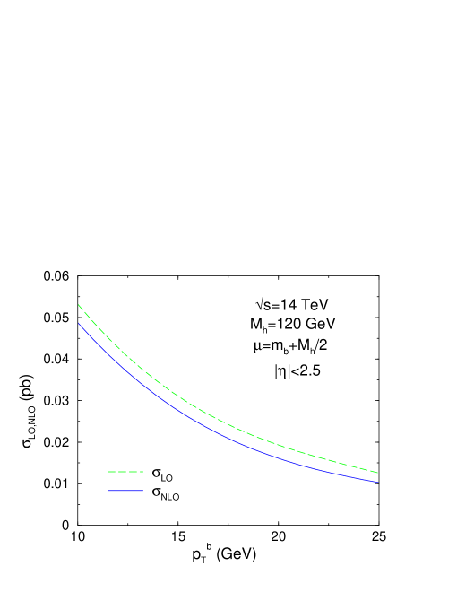
Figure 4: $\sigma_{\scriptscriptstyle NLO,MS}$ and $\sigma_{\scriptscriptstyle LO,MS}$ for $p\bar{p}\to b\bar{b}h$ at $\sqrt{s}\!=\!2$ TeV (top) and for $pp\to b\bar{b}h$ at $\sqrt{s}\!=\!14$ TeV (bottom) as a function of the cut imposed on the final state bottom and anti-bottom transverse momentum ($p_{T}^{b}$), for $M_{h}\!=\!120$ GeV and $\mu\!=\!\mu_{0}\!=\!m_{b}+M_{h}/2$.

Our numerical results are obtained using CTEQ5M parton distribution functions for the calculation of the NLO cross section, and CTEQ5L parton distribution functions for the calculation of the lowest order cross section Lai et al. (2000). The NLO (LO) cross section is evaluated using the 2-loop (1-loop) evolution of $\alpha_{s}(\mu)$ with $\alpha_{s}^{NLO}(M_{Z})=0.118$. The bottom quark pole mass is taken to be $m_{b}\!=\!4.6$ GeV. In the OS scheme the bottom quark Yukawa coupling is calculated as $g_{b\bar{b}h}\!=\!m_{b}/v$, while in the $\overline{MS}$ scheme as $g_{b\bar{b}h}(\mu)\!=\!\overline{m}_{b}(\mu)/v$, where we use $\overline{m}_{b}(\mu)_{1l}$ from Eq. (13) for $\sigma_{\scriptscriptstyle LO}$ and $\overline{m}_{b}(\mu)_{2l}$ from Eq. (II.2) for $\sigma_{\scriptscriptstyle NLO}$.

We evaluate the fully exclusive LO and NLO cross sections for $b\bar{b}h$ production by requiring that the transverse momentum of both final state bottom and anti-bottom quarks be larger than 20 GeV ($p_{T}^{b}\!>\!20$ GeV), and that their pseudorapidity satisfy the condition $|\eta_{b}|\!<\!2$ for the Tevatron and $|\eta_{b}|\!<\!2.5$ for the LHC. This corresponds to an experiment measuring the Higgs decay products along with two high $p_{T}$ bottom quark jets that are clearly separated from the beam. Furthermore, we present LO and NLO transverse momentum and pseudorapidity distributions. In order to better simulate the detector response, the gluon and the bottom/anti-bottom quarks are treated as distinct particles only if the separation in the azimuthal angle-pseudorapidity plane is $\Delta R\!>\!0.4$. For smaller values of $\Delta R$, the four momentum vectors of the two particles are combined into an effective bottom/anti-bottom quark momentum four-vector.

III.1 Standard Model Results

In Fig. 2 we show, for $M_{h}\!=\!120$ GeV, the dependence of the LO and NLO cross sections for $p\bar{p}\to b\bar{b}h$ at the Tevatron (top) and for $pp\to b\bar{b}h$ at the LHC (bottom) on the unphysical factorization and renormalization scale, $\mu$, when using either the $OS$ or the $\overline{MS}$ renormalization schemes for the bottom quark Yukawa coupling. In both the $OS$ and $\overline{MS}$ schemes the stability of the cross section is greatly improved at NLO, given the much milder scale dependence with respect to the corresponding LO cross section. The results presented in Fig. 2 are obtained by setting $\mu\!=\!\mu_{r}\!=\!\mu_{f}$, i.e. by identifying the renormalization ($\mu_{r}$) and factorization ($\mu_{f}$) scales. We have checked that varying them independently does not affect the results significantly. By varying the scale $\mu$ in the ranges $0.7\mu_{0}<\mu<4\mu_{0}$ (Tevatron) and $0.5\mu_{0}<\mu<8\mu_{0}$ (LHC), when using the $OS$ scheme for the bottom quark Yukawa coupling, and in the ranges $0.4\mu_{0}<\mu<2\mu_{0}$ (Tevatron) and $0.2\mu_{0}<\mu<2\mu_{0}$ (LHC) when using the $\overline{MS}$ scheme, i. e. in the plateau regions, the value of the NLO cross section varies by at most 15-20% (where $\mu_{0}\!=\!m_{b}+M_{h}/2$) .

As can be seen in Fig. 2, the cross section calculated with $g_{b\bar{b}h}$ in the $\overline{MS}$ scheme shows a better perturbative behavior, since the difference between $\sigma_{\scriptscriptstyle LO}$ and $\sigma_{\scriptscriptstyle NLO}$ is smaller. This is in part due to the fact that the LO cross section is calculated using $\overline{m}_{b}(\mu)_{1l}$ and therefore already contains some of the corrections from the renormalization of the bottom quark Yukawa coupling that appear in the NLO cross section as well as at higher order. This observation seems to justify the use of $\overline{m}_{b}(\mu)_{1l}$ at LO and $\overline{m}_{b}(\mu)_{2l}$ at NLO. One also observes that the $\overline{MS}$ NLO cross section is better behaved at low values of the renormalization/factorization scales. At the same time, both the $OS$ and $\overline{MS}$ cross sections show well defined but distinct regions of least sensitivity to the renormalization/factorization scale. In both cases this happens in the region where the LO and NLO cross section are closer. The variation of the NLO cross section with $\mu$ about its point of least sensitivity to the renormalization/factorization scale is almost the same whether one uses the $OS$ or $\overline{MS}$ schemes for the bottom quark Yukawa coupling. This indicates that the running of the Yukawa coupling is not the only important factor to determine the overall perturbative stability of the NLO cross section.

As discussed in Section II.2, the numerical difference between the two renormalization schemes can be significant. This is illustrated in Fig. 3 where we plot the absolute values of the relative difference, $\Delta\!=\!(\sigma_{\scriptscriptstyle NLO,OS}-\sigma_{\scriptscriptstyle NLO,\overline{MS}})/(\sigma_{\scriptscriptstyle NLO,OS}+\sigma_{\scriptscriptstyle NLO,\overline{MS}})$, between the hadronic cross sections $\sigma_{\scriptscriptstyle NLO,OS}$ and $\sigma_{\scriptscriptstyle NLO,\overline{MS}}$ at both the Tevatron and the LHC. As discussed in detail at the parton level in Section II.2 (see $\hat{\Delta}$ defined in Eq.(19)), the difference between the two schemes is scale dependent and can be very big for small and large scales. At the LHC, the relative difference can be well approximated by $\Delta=\frac{\displaystyle 1}{\displaystyle 2}AB$ with $A=\frac{\displaystyle\alpha_{s}}{\displaystyle 4\pi}g_{\scriptscriptstyle NLO}/g_{\scriptscriptstyle LO}$ and $B=(1-(\overline{m}_{b}/m_{b})^{2})$, where $g_{\scriptscriptstyle NLO,\scriptscriptstyle LO}$ correspond to the $g_{\scriptscriptstyle NLO,\scriptscriptstyle LO}^{ij}$ contributions of Eqs. (II.2) and (18) calculated at hadron level. For instance, at $\mu=0.7\mu_{0}$, $A=0.28$ and $B=0.57$, while at $\mu=4\mu_{0}$, $A=0.92$ and $B=0.66$, which shows that the difference between the $\overline{MS}$ and the $OS$ schemes of the bottom quark is not dominated by the running of the bottom quark mass as it would be the case when the majority of the NLO corrections can be absorbed in the running of $m_{b}$.

From both the observed similar scale dependence of $\sigma_{\scriptscriptstyle NLO}$ in both schemes and the large numerical difference due to the corrections that cannot be absorbed in the running of $m_{b}$, we conclude that the use of the $\overline{MS}$ bottom quark Yukawa coupling should probably not be overemphasized. It is probably a good approximation to take the difference between $\sigma_{\scriptscriptstyle NLO,OS}$ and $\sigma_{\scriptscriptstyle NLO,\overline{MS}}$ at their points of least scale sensitivity as an upper bound on the theoretical error of the NLO cross section, on top of the uncertainty due to the residual scale dependence. This would amount to an additional 15-20% uncertainty arising from the dependence on the bottom quark Yukawa coupling renormalization scheme.

In Fig. 4 we illustrate the dependence of the exclusive cross section on the $p_{T}$ cut imposed on the final state bottom and anti-bottom quarks, at both the Tevatron (top) and the LHC (bottom). We plot the LO and NLO cross sections obtained using the $\overline{MS}$ bottom quark Yukawa coupling. Reducing the $p_{T}$ cut from 25 GeV to 10 GeV approximately increases the cross section by a factor of four. However, as the $p_{T}$ cut is reduced, the theoretical calculation of the cross section becomes more unstable, because the integration over the phase space of the final state bottom quarks approaches more and more a region of collinear singularities. Results without a cut on the transverse momentum of the bottom quarks will be presented in a later work Dawson et al. (see also Ref. Dittmaier et al. (2003)).

Finally, in Figs. 5, 6, 7, and 8 we plot the LO and NLO transverse momentum ($p_{T}$) and pseudorapidity ($\eta$) distributions of the final state particles, the bottom and anti-bottom quarks and the Higgs boson, both for the Tevatron and for the LHC. Both LO and NLO differential cross sections are obtained in the SM and using the $OS$ scheme for the bottom quark Yukawa coupling. For the renormalization/factorization scale we choose $\mu=2m_{b}+M_{h}$ at the Tevatron and $\mu=2(2m_{b}+M_{h})$ at the LHC. These two scales are well within the plateau regions where the $OS$ NLO cross sections vary the least with the value of $\mu$. Similar results can be obtained using the $\overline{MS}$ bottom quark Yukawa coupling.

In Fig. 5 we show the LO and NLO $p_{T}$ distributions of the bottom or anti-bottom quark with highest $p_{T}$, while Fig. 6 displays the $p_{T}$ distributions of the SM Higgs boson. The pseudorapidity distributions of the bottom quark and the Higgs boson are shown in Fig. 7 and Fig. 8, respectively. The inclusion of the NLO corrections causes the cross sections to be more sharply peaked around low $p_{T}^{b,h}$ and around $\eta_{b,h}\!=\!0$.

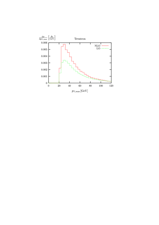
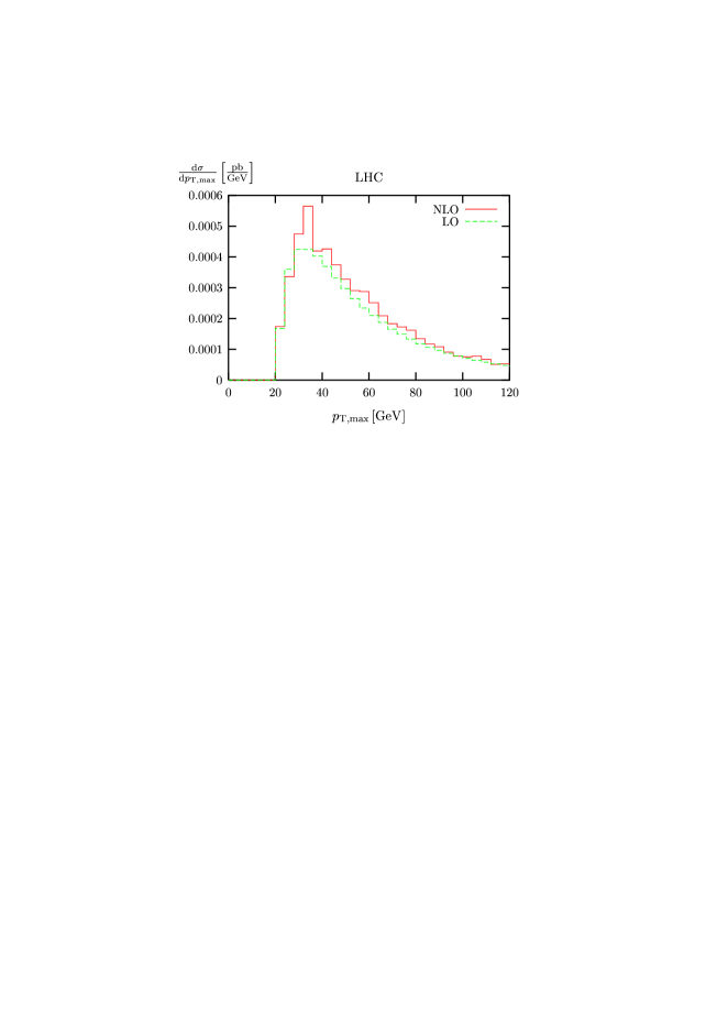
Figure 5: Transverse momentum distributions at LO and NLO of the bottom or anti-bottom quark with the largest $p_{T}$. Shown are the $p_{T}^{max}$ distributions for $p\bar{p}\to b\bar{b}h$ production at $\sqrt{s}\!=\!2$ TeV (left) and $pp\to b\bar{b}h$ production at $\sqrt{s}\!=\!14$ TeV (right) in the SM and using the OS scheme for the bottom quark Yukawa coupling. At the Tevatron we choose $\mu\!=\!2m_{b}+M_{h}$, while at the LHC we choose $\mu\!=\!2(2m_{b}+M_{h})$.

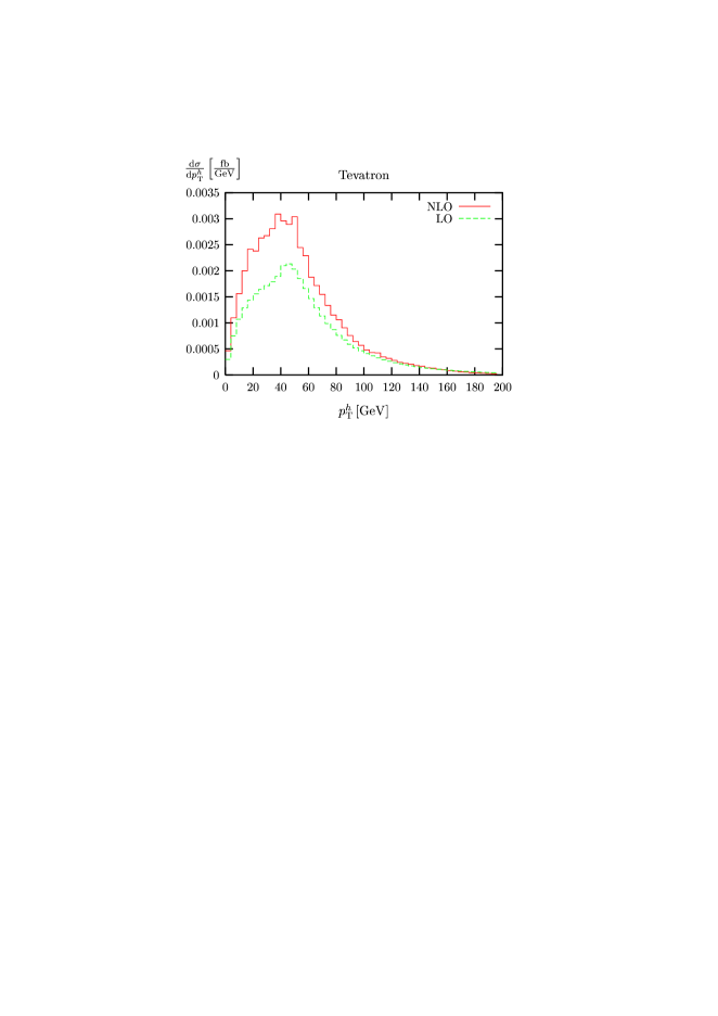
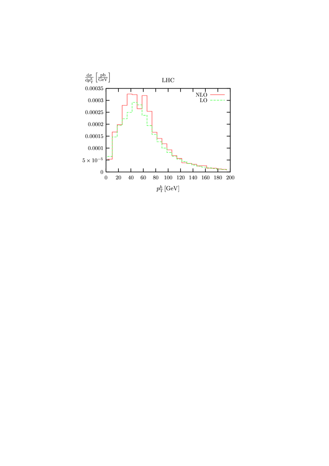
Figure 6: Transverse momentum distributions at LO and NLO of the SM Higgs boson. Shown are the $p_{T}^{h}$ distributions for $p\bar{p}\to b\bar{b}h$ production at $\sqrt{s}\!=\!2$ TeV (left) and $pp\to b\bar{b}h$ production at $\sqrt{s}\!=\!14$ TeV (right) in the SM and using the OS scheme for the bottom quark Yukawa coupling. At the Tevatron we choose $\mu\!=\!2m_{b}+M_{h}$, while at the LHC we choose $\mu\!=\!2(2m_{b}+M_{h})$.

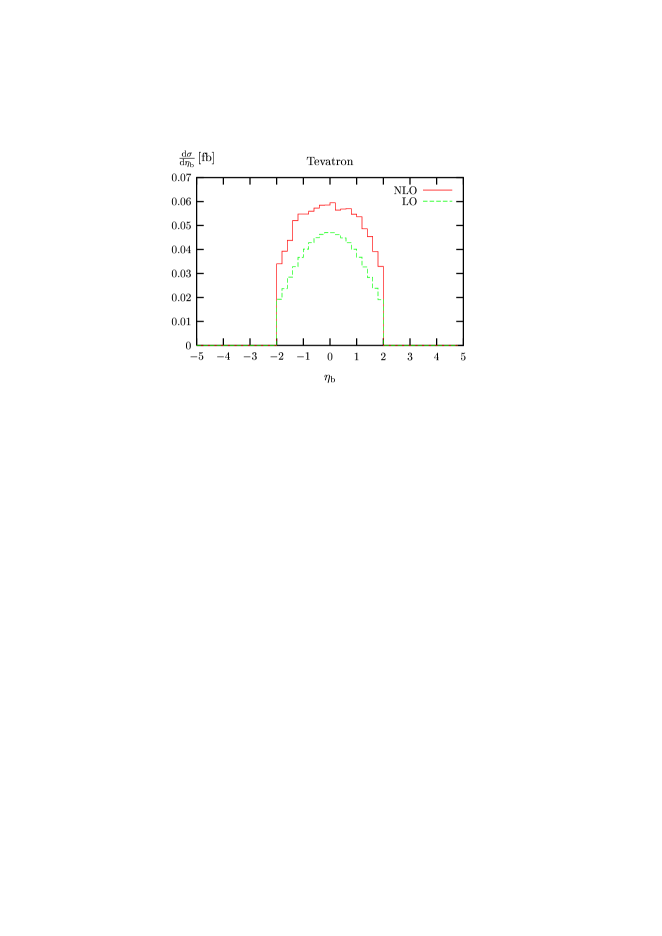
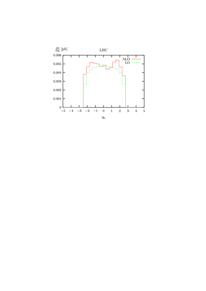
Figure 7: Pseudorapidity distributions at LO and NLO of the bottom quark. Shown are the $\eta_{b}$ distributions for $p\bar{p}\to b\bar{b}h$ production at $\sqrt{s}\!=\!2$ TeV (left) and $pp\to b\bar{b}h$ production at $\sqrt{s}\!=\!14$ TeV (right) in the SM and using the OS scheme for the bottom quark Yukawa coupling. At the Tevatron we choose $\mu=2m_{b}+M_{h}$, while at the LHC we choose $\mu=2(2m_{b}+M_{h})$.

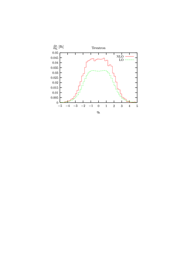
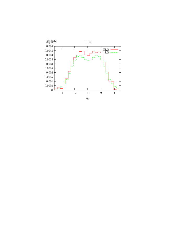
Figure 8: Pseudorapidity distributions at LO and NLO of the SM Higgs boson. Shown are the $\eta_{h}$ distributions for $p\bar{p}\to b\bar{b}h$ production at $\sqrt{s}\!=\!2$ TeV (left) and $pp\to b\bar{b}h$ production at $\sqrt{s}\!=\!14$ TeV (right) in the SM and using the OS scheme for the bottom quark Yukawa coupling. At the Tevatron we choose $\mu=2m_{b}+M_{h}$, while at the LHC we choose $\mu=2(2m_{b}+M_{h})$.

III.2 MSSM Results

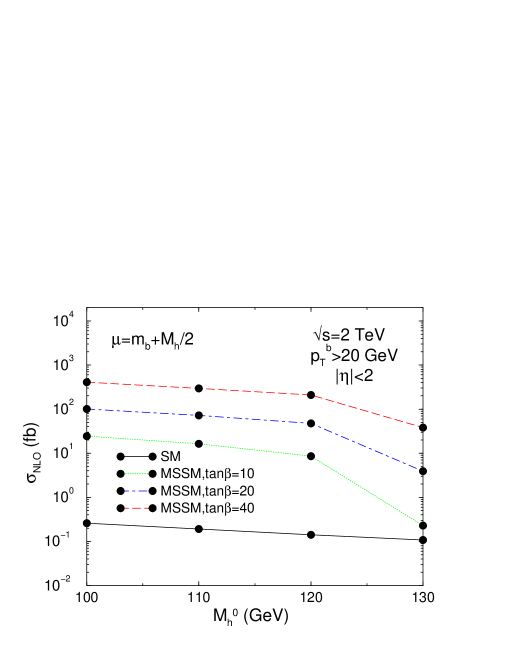
Figure 9: $\sigma_{\scriptscriptstyle NLO,MS}$ for $p\bar{p}\to b\bar{b}h$ production at $\sqrt{s}\!=\!2$ TeV (top) and $pp\to b\bar{b}h$ production at $\sqrt{s}\!=\!14$ TeV (bottom) in the SM and in the MSSM with $\tan\beta\!=\!10,20$, and $40$. For the Tevatron we considered $p\bar{p}\to b\bar{b}h^{0}$ with $M_{h^{0}}\!=\!100,110,120$, and 130 GeV, while for the LHC we considered $pp\to b\bar{b}H^{0}$ with $M_{H^{0}}\!=\!120,200,400,600$, and 800 GeV. For each $(M_{h^{0}},\tan\beta)$ and $(M_{H^{0}},\tan\beta)$ point, the corresponding values of $\alpha$ and $M_{A}$ are listed in Tables 1 and 2.

The rate for $b\bar{b}h$ production can be significantly enhanced in a supersymmetric model with large values of $\tan\beta$. In the MSSM, the bottom and top quark couplings to the scalar Higgs bosons are given by:

$$\begin{array}[]{lclrcr}b\bar{b}h^{0}&:&-\displaystyle{\frac{\sin\alpha}{\cos\beta}}g_{b\bar{b}h}&\;\;\;t\bar{t}h^{0}&:&\;\;\displaystyle{\frac{\cos\alpha}{\sin\beta}}g_{t\bar{t}h}\\ b\bar{b}H^{0}&:&\;\;\displaystyle{\frac{\cos\alpha}{\cos\beta}}g_{b\bar{b}h}&\;\;\;t\bar{t}H^{0}&:&\;\;\displaystyle{\frac{\sin\alpha}{\sin\beta}}g_{t\bar{t}h}\end{array}$$

where $g_{b\bar{b}h}$ and $g_{t\bar{t}h}$ are the SM bottom and top quark Yukawa couplings, $h^{0}$ and $H^{0}$ are the lighter and heavier neutral scalars of the MSSM, and $\alpha$ is the angle which diagonalizes the neutral scalar Higgs mass matrix Gunion et al. (1990). By replacing the SM top and bottom quark Yukawa couplings with the corresponding MSSM ones, our calculation can then be straightforwardly generalized to the case of the scalar Higgs bosons of the MSSM. The bottom quark Yukawa coupling to the MSSM pseudoscalar Higgs boson, $A^{0}$, is also enhanced at large $\tan\beta$. The corresponding cross section for $b\bar{b}A^{0}$ production can be obtained from our calculation in the $m_{b}\to 0$ limit, which we do not consider in this paper. We will present, however, complete results for $b\bar{b}A^{0}$ production, i. e. for non-zero $m_{b}$, in a future study.

The MSSM Higgs boson masses and the mixing angle $\alpha$ have been computed up to two-loop order using the program FeynHiggs Heinemeyer et al. (2000). In Tables 1 and 2 we provide the values of the input parameters ($(M_{h^{0}},\tan\beta)$ or $(M_{H^{0}},\tan\beta)$) and the resulting values of $\alpha$ used in the calculation of the top and bottom quark Yukawa couplings to the light and heavy neutral MSSM scalar Higgs bosons. This choice of MSSM parameters takes into account present experimental limits on the MSSM parameter space, but represents otherwise just one among many possible realizations of the MSSM parameter space. The results obtained with this choice of MSSM input parameters illustrate the typical enhancements over the SM results one can expect when considering the production of neutral scalar Higgs bosons in association with bottom quarks.

$\tan\beta=10$
$M_{h^{0}}$ [GeV]	100	110	120	130
$M_{A}$ [GeV]	102.42	113.86	127.95	264.72
$\alpha$ [rad]	-1.3249	-1.1963	-0.9054	-0.1463
$\tan\beta=20$
$M_{h^{0}}$ [GeV]	100	110	120	130
$M_{A}$ [GeV]	100.61	110.95	121.89	146.72
$\alpha$ [rad]	-1.4420	-1.3707	-1.1856	-0.3108
$\tan\beta=40$
$M_{h^{0}}$ [GeV]	100	110	120	130
$M_{A}$ [GeV]	100.15	110.23	120.46	133.71
$\alpha$ [rad]	-1.5007	-1.4601	-1.3444	-0.4999

Table 1: Values of $\alpha$ and $M_{A}$, computed up to two-loop order by using the program FeynHiggs Heinemeyer et al. (2000), corresponding to different choices of $\tan\beta$ and $M_{h^{0}}$. In the calculation of $\alpha$ and $M_{A}$ we choose the genuine SUSY input parameters as follows: $M_{\tilde{g}}\!=\!M_{\tilde{t}_{L}}\!=\!M_{\tilde{t}_{R}}\!=\!M_{\tilde{b}_{L}}\!=\!M_{\tilde{b}_{R}}\!=\!1$ TeV, $M_{t}^{LR}\!=\!2$ TeV, $A_{b}\!=\!A_{t}\!=\!M_{t}^{LR}+\mu\cot\beta$, and $\mu\!=\!M_{2}\!=\!200$ GeV.

The top part of Fig. 9 compares the NLO $p\bar{p}\to b\bar{b}h$ SM cross section at the Tevatron with the corresponding cross section for production of the lightest neutral scalar Higgs boson in the MSSM for $\tan\beta=10,20$, and $40$. A large enhancement of up to three orders of magnitude is observed. As the light neutral Higgs boson mass approaches its maximum value, the mixing angle $\alpha$ becomes very small, as can be clearly seen in Table 1. This has the effect of suppressing the $b\bar{b}h^{0}$ rates at this point. A similar effect can be observed in the production of a heavy neutral Higgs boson when $M_{H^{0}}$ is approaching its minimum value (see Table 2), as shown in the bottom part of Fig. 9. Again, we compare the production of the SM Higgs boson with that of the heavier neutral scalar Higgs boson of the MSSM and observe a significant enhancement of the rate in the MSSM for large $\tan\beta$.

$\tan\beta=10$
$M_{H^{0}}$ [GeV]	120	200	400	600	800
$M_{A}$ [GeV]	108.05	198.55	399.41	599.64	799.74
$\alpha$ [rad]	-0.9018	-0.1762	-0.1140	-0.1057	-0.1030
$\tan\beta=20$
$M_{H^{0}}$ [GeV]	120	200	400	600	800
$M_{A}$ [GeV]	116.45	199.56	399.81	599.89	799.91
$\alpha$ [rad]	-0.5785	-0.0901	-0.0574	-0.0531	-0.0517
$\tan\beta=40$
$M_{H^{0}}$ [GeV]	120	200	400	600	800
$M_{A}$ [GeV]	118.92	199.82	399.92	599.95	799.96
$\alpha$ [rad]	-0.3116	-0.0460	-0.0289	-0.0267	-0.0259

Table 2: Values of $\alpha$ and $M_{A}$, computed up to two-loop order by using the program FeynHiggs Heinemeyer et al. (2000), corresponding to different choices of $\tan\beta$ and $M_{H^{0}}$. In the calculation of $\alpha$ and $M_{A}$ we choose the genuine SUSY input parameters as follows: $M_{\tilde{g}}=M_{\tilde{t}_{L}}=M_{\tilde{t}_{R}}=M_{\tilde{b}_{L}}=M_{\tilde{b}_{R}}=1$ TeV, $M_{t}^{LR}=0$, $A_{b}=A_{t}=M_{t}^{LR}+\mu\cot\beta$, and $\mu=M_{2}=1$ TeV.

IV Conclusions

We presented results for the next-to-leading order QCD cross section for exclusive $b\bar{b}h$ production at both the Tevatron and the LHC. Our NLO results show an improved stability with respect to the unphysical factorization and renormalization scales as compared to the leading order results and increase the reliability of the theoretical prediction. The uncertainty in the resummation of large logarithms from higher order corrections, however, is also visible in the dependence of the NLO cross section on the renormalization scheme of the bottom quark Yukawa coupling. The residual renormalization/factorization scale dependence is of the order of 15-20% when the bottom quark Yukawa coupling is renormalized in the $OS$ or $\overline{MS}$ schemes respectively. We conservatively estimate the additional uncertainty due to the renormalization scheme dependence of the bottom quark Yukawa coupling to be at most of order 15-20%.

Our calculation is important for Higgs boson searches at hadron colliders where two high $p_{T}$ bottom quarks are tagged in the final state. In supersymmetric models with large $\tan\beta$, $b\bar{b}h$ production can be an important discovery channel, at both the Tevatron and the LHC.

References

- LEP Higgs Working Group (2003) LEP Higgs Working Group, Phys. Lett. B 565, 61 (2003), CERN-EP/2003-011, eprint hep-ex/0306033.
- (2) LEP Electroweak Working Group, talk presented by P. Wells, EPS-HEP Conference, Aachen, Germany, July 2003. See also LEP EWWG web site at http://lepewwg.web.cern.ch/LEPEWWG/.
- LEP Higgs Working Group (July 2001) LEP Higgs Working Group (July 2001), Note/2001-04, eprint hep-ex/0107030.
- Han and Willenbrock (1991) T. Han and S. Willenbrock, Phys. Lett. B273, 167 (1991).
- Han et al. (1992) T. Han, G. Valencia, and S. Willenbrock, Phys. Rev. Lett. 69, 3274 (1992), eprint hep-ph/9206246.
- Dawson (1991) S. Dawson, Nucl. Phys. B359, 283 (1991).
- Djouadi et al. (1991) A. Djouadi, M. Spira, and P. M. Zerwas, Phys. Lett. B264, 440 (1991).
- Graudenz et al. (1993) D. Graudenz, M. Spira, and P. M. Zerwas, Phys. Rev. Lett. 70, 1372 (1993).
- Spira et al. (1995) M. Spira, A. Djouadi, D. Graudenz, and P. M. Zerwas, Nucl. Phys. B453, 17 (1995), eprint hep-ph/9504378.
- Beenakker et al. (2001) W. Beenakker, S. Dittmaier, M. Krämer, B. Plümper, M. Spira, and P. Zerwas, Phys. Rev. Lett. 87, 201805 (2001), eprint hep-ph/0107081.
- Reina and Dawson (2001) L. Reina and S. Dawson, Phys. Rev. Lett. 87, 201804 (2001), eprint [http://arXiv.org/abs]hep-ph/0107101.
- Beenakker et al. (2003) W. Beenakker, S. Dittmaier, M. Krämer, B. Plümper, M. Spira, and P. Zerwas, Nucl. Phys. B653, 151 (2003), eprint hep-ph/0211352.
- Reina et al. (2002) L. Reina, S. Dawson, and D. Wackeroth, Phys. Rev. D65, 053017 (2002), eprint [http://arXiv.org/abs]hep-ph/0109066.
- Dawson et al. (2003a) S. Dawson, L. H. Orr, L. Reina, and D. Wackeroth, Phys. Rev. D67, 071503 (2003a), eprint hep-ph/0211438.
- Dawson et al. (2003b) S. Dawson, C. Jackson, L. H. Orr, L. Reina, and D. Wackeroth, Phys. Rev. D68, 034022 (2003b), eprint hep-ph/0305087.
- Harlander and Kilgore (2002) R. V. Harlander and W. B. Kilgore, Phys. Rev. Lett. 88, 201801 (2002), eprint hep-ph/0201206.
- Anastasiou and Melnikov (2002) C. Anastasiou and K. Melnikov, Nucl. Phys. B646, 220 (2002), eprint hep-ph/0207004.
- Harlander and Kilgore (2001) R. V. Harlander and W. B. Kilgore, Phys. Rev. D64, 013015 (2001), eprint hep-ph/0102241.
- Catani et al. (2001) S. Catani, D. de Florian, and M. Grazzini, JHEP 05, 025 (2001), eprint hep-ph/0102227.
- Ravindran et al. (2002) V. Ravindran, J. Smith, and W. L. Van Neerven, Nucl. Phys. B634, 247 (2002), eprint hep-ph/0201114.
- Brein et al. (2003) O. Brein, A. Djouadi, and R. Harlander (2003), eprint hep-ph/0307206.
- Dicus and Willenbrock (1989) D. A. Dicus and S. Willenbrock, Phys. Rev. D39, 751 (1989).
- Harlander and Kilgore (2003) R. V. Harlander and W. B. Kilgore, Phys. Rev. D68, 013001 (2003), eprint hep-ph/0304035.
- Dicus et al. (1999) D. Dicus, T. Stelzer, Z. Sullivan, and S. Willenbrock, Phys. Rev. D59, 094016 (1999), eprint hep-ph/9811492.
- Balazs et al. (1999a) C. Balazs, H.-J. He, and C. P. Yuan, Phys. Rev. D60, 114001 (1999a), eprint hep-ph/9812263.
- Rainwater et al. (2002) D. Rainwater, M. Spira, and D. Zeppenfeld (2002), eprint hep-ph/0203187.
- Plehn (2003) T. Plehn, Phys. Rev. D67, 014018 (2003), eprint hep-ph/0206121.
- Maltoni et al. (2003) F. Maltoni, Z. Sullivan, and S. Willenbrock, Phys. Rev. D67, 093005 (2003), eprint hep-ph/0301033.
- Boos and Plehn (2003) E. Boos and T. Plehn (2003), eprint hep-ph/0304034.
- (30) Talk presented by M. Krämer, Workshop on the Physics of TeV Colliders, Les Houches, France, May 2003.
- (31) Talk presented by M. Spira, CERN Workshop on Monte Carlo tools for the LHC, CERN, Geneva, Switzerland, July 2003.
- Dittmaier et al. (2003) S. Dittmaier, M. Krämer, and M. Spira (2003), eprint hep-ph/0309204.
- CMS Collaboration (1994) CMS Collaboration (1994), Technical Proposal, eprint CERN/LHCC/94-38.
- Barger and Kao (1998) V. D. Barger and C. Kao, Phys. Lett. B424, 69 (1998), eprint hep-ph/9711328.
- Richter-Was et al. (1998) E. Richter-Was et al., Int. J. Mod. Phys. A13, 1371 (1998).
- ATLAS Collaboration (1999) ATLAS Collaboration (1999), Technical Design Report, Vol. II, eprint CERN/LHCC/99-15.
- Carena et al. (1999) M. Carena, S. Mrenna, and C. E. M. Wagner, Phys. Rev. D60, 075010 (1999), eprint hep-ph/9808312.
- Campbell et al. (2003) J. Campbell, R. K. Ellis, F. Maltoni, and S. Willenbrock, Phys. Rev. D67, 095002 (2003), eprint hep-ph/0204093.
- Dai et al. (1995) J. Dai, J. F. Gunion, and R. Vega, Phys. Lett. B345, 29 (1995), eprint hep-ph/9403362.
- Dai et al. (1996) J. Dai, J. F. Gunion, and R. Vega, Phys. Lett. B387, 801 (1996), eprint hep-ph/9607379.
- Affolder et al. (2001) T. Affolder et al. (CDF), Phys. Rev. Lett. 86, 4472 (2001), eprint hep-ex/0010052.
- Carena et al. (2000) M. Carena et al. (Report of the Tevatron Higgs Working Group) (2000), eprint hep-ph/0010338.
- Balazs et al. (1999b) C. Balazs, J. L. Diaz-Cruz, H. J. He, T. Tait, and C. P. Yuan, Phys. Rev. D59, 055016 (1999b), eprint hep-ph/9807349.
- Richter-Was and Froidevaux (1997) E. Richter-Was and D. Froidevaux, Z. Phys. C76, 665 (1997), eprint hep-ph/9708455.
- Dawson et al. (2002) S. Dawson, D. Dicus, and C. Kao, Phys. Lett. B545, 132 (2002), eprint hep-ph/0208063.
- Boos et al. (2003) E. Boos, A. Djouadi, and A. Nikitenko (2003), eprint hep-ph/0307079.
- Braaten and Leveille (1980) E. Braaten and J. P. Leveille, Phys. Rev. D22, 715 (1980).
- Drees and Hikasa (1990) M. Drees and K.-i. Hikasa, Phys. Lett. B240, 455 (1990).
- Gorishnii et al. (1984) S. G. Gorishnii, A. L. Kataev, and S. A. Larin, Sov. J. Nucl. Phys. 40, 329 (1984).
- Kataev and Kim (1994) A. L. Kataev and V. T. Kim, Mod. Phys. Lett. A9, 1309 (1994).
- (51) Talks presented by L. Reina, Workshop on the Physics of TeV Colliders, Les Houches, France, May 2003; QCD 2003, Montpelleier, France, July 2003; EPS 2003, Aachen, Germany, July 2003.
- Collins et al. (1978) J. C. Collins, F. Wilczek, and A. Zee, Phys. Rev. D18, 242 (1978).
- Nason et al. (1989) P. Nason, S. Dawson, and R. K. Ellis, Nucl. Phys. B327, 49 (1989).
- Lehmann et al. (1955) H. Lehmann, K. Symanzik, and W. Zimmermann, Nuovo Cim. 1, 205 (1955).
- Altarelli and Parisi (1977) G. Altarelli and G. Parisi, Nucl. Phys. B126, 298 (1977).
- Lai et al. (2000) H. L. Lai et al. (CTEQ), Eur. Phys. J. C12, 375 (2000), eprint hep-ph/9903282.
- (57) S. Dawson, C. Jackson, L. Reina, and D. Wackeroth, in preparation.
- Gunion et al. (1990) J. F. Gunion, H. E. Haber, G. L. Kane, and S. Dawson, The Higgs Hunter’s Guide (Addison-Wesley, Menlo Park) (1990), SCIPP-89/13.
- Heinemeyer et al. (2000) S. Heinemeyer, W. Hollik, and G. Weiglein, Comput. Phys. Commun. 124, 76 (2000), we used version 1.3.1 (December 2002). For details see FeynHiggs web site at http://www.feynhiggs.de/FeynHiggs.html, eprint hep-ph/9812320.