$H^{\pm}W^{\mp}Z$ contribution to the static quantities of the $W$ boson in the context of Higgs-triplet theories

Abstract

We calculate the one–loop contribution from the $H^{\pm}W^{\mp}Z$ coupling to the static electromagnetic properties of the $W$ boson. Although this coupling is absent at the tree–level in all Higgs–doublet models, it can be induced at this order in models including Higgs–triplet representations. It is found that the $H^{\pm}W^{\mp}Z$ contribution can be as important as those arising from other couplings including Higgs bosons, such as the standard model coupling $W^{\pm}W^{\mp}H$ or the two–Higgs–doublet model couplings $H^{\pm}W^{\mp}\phi^{0}$ and $W^{\pm}W^{\mp}\phi^{0}$, with $\phi^{0}=h,\,H$ and $A$.

I Introduction

The trilinear gauge boson couplings $W^{\pm}W^{\mp}\gamma$ and $W^{\pm}W^{\mp}Z$ are representative of the nonabelian structure of the standard model (SM). It is thus interesting to study any anomalous (one–loop) contribution to them as it is important to test the quantization procedures used for these nonabelian gauge systems. In this context, the CP–even static electromagnetic properties of the $W$ boson, which are parametrized by two form factors, $\Delta\kappa$ and $\Delta Q$, have been the subject of considerable interest in the literature as is expected that future particle colliders be sensitive to this class of effects Diehl . The SM contributions to $\Delta\kappa$ and $\Delta Q$ were calculated in Ref. Bardeen for massless fermions, and the top quark contribution was presented in Top . The sensitivity of these quantities to new physics effects has also been analyzed in some SM extensions, such as the two–Higgs–doublet model (THDM) THDM , supersymmetric theories SUSY , left–right symmetric models Roberto , $SU(3)\times SU(3)\times U(1)$ modelsTT , and models with composite particles Rizzo and an extra gauge boson $Z^{\prime}$ Sharma . $\Delta\kappa$ and $\Delta Q$ have also been parametrized in a model independent manner by using the effective Lagrangian technique EL . In this work we present the calculation of the contribution from the $H^{\pm}W^{\mp}Z$ coupling to the static quantities of the $W$ boson. Charged Higgs bosons appear in many extensions of the SM, such as the popular THDM. In the search for a charged Higgs boson, the $H^{\pm}W^{\mp}Z$ coupling might play an important role, although it is expected to be very suppressed in a Higgs–doublet model. In fact, although the $H^{\pm}W^{\mp}Z$ coupling can have a renormalizable structure, it can only be generated at the one-loop level in multi–Higgs–doublet models HWZ . Nevertheless, it can be induced at the tree–level in theories with Higgs triplets or higher representations, though it could be severely constrained by the $\rho$ parameter. This is true in some Higgs–triplet models which do not respect the $SU(2)$ custodial symmetry HHG ; GM . It is possible however to construct a model including Higgs triplets that does respect such a custodial symmetry G ; CG ; GVW , thereby relaxing the constraints from the $\rho$ parameter. The phenomenology of the $H^{\pm}W^{\mp}Z$ coupling has been investigated in the context of the CERN $e^{+}e^{-}$ LEP–II collider, the next linear collider LC , and hadronic colliders HC . Such studies focus mainly on discriminating a charged Higgs bosons arising from a model with Higgs triplets from that induced by a Higgs–doublet model. The main goal of this work is to study the impact of the $H^{\mp}W^{\mp}Z$ vertex on the static electromagnetic properties of the $W$ boson. We will show that the respective contributions to $\Delta\kappa$ and $\Delta Q$ may be of the same order of magnitude as those arising from other renormalizable theories which include neutral o charged Higgs bosons, such as the SM or the THDM.

The rest of the paper is organized as follows. In Sec. II we present the calculation of the $\Delta\kappa$ and $\Delta Q$ form factors. Sec. III is devoted to discuss the numerical results. Finally, the conclusions are presented in Sec. IV.

II $H^{\pm}W^{\mp}Z$ contribution to the on–shell $W^{\pm}W^{\mp}\gamma$ vertex

Using the momenta depicted in Fig. 1, the most general CP–even Lorentz structure for the on–shell $W^{\pm}W^{\mp}\gamma$ vertex can be written as

$$\Gamma_{\alpha\beta\mu}=ie\left(A\left(2p_{\mu}g_{\alpha\beta}+4(q_{\beta}g_{\alpha\mu}-q_{\alpha}g_{\beta\mu})\right)+2\Delta\kappa(q_{\beta}g_{\alpha\mu}-q_{\alpha}g_{\beta\mu})+\frac{4\Delta Q}{m^{2}_{W}}p_{\mu}q_{\alpha}q_{\beta}\right).$$ (1)

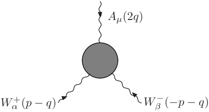
Figure 1: Trilinear $W^{\pm}W^{\mp}\gamma$ coupling. The loop denotes contributions from charged particles.

In the SM, both $\Delta\kappa$ and $\Delta Q$ vanish at the tree–level, whereas the one–loop corrections are of the order of $\alpha/\pi$. These parameters define the magnetic dipole moment $\mu_{W}$ and the electric quadrupole moment $Q_{W}$ of the $W$ boson:

$$\mu_{W} = \frac{e}{2m_{W}}(2+\Delta\kappa),$$ (2)

$$Q_{W} = -\frac{e}{m^{2}_{W}}(1+\Delta\kappa+\Delta Q).$$ (3)

It is worth discussing the origin of the $H^{\pm}W^{\mp}Z$ vertex. It has the following renormalizable structure which is dictated by Lorentz covariance

$$i\,s_{H}\,g\,m_{Z}\,g_{\mu\nu},$$ (4)

where $s_{H}$ is a model–dependent quantity which may be very suppressed in models containing only Higgs doublets HWZ . As pointed out before, in models with a scalar sector including doublets and triplets, $s_{H}$ may be considerably enhanced since the $H^{\pm}W^{\mp}Z$ vertex is induced at the tree–level. However, not any scalar sector including triplets or higher representations is viable due to the fact that large deviations from the tree–level relation $\rho=1$ may arise. One possibility is to invoke a tree–level custodial $SU(2)$ symmetry respected by the Higgs sector, which guarantees that $\rho=1$ at the tree–level. In this case, the existence of a tree–level–induced $H^{\pm}W^{\mp}Z$ vertex with strength $s_{H}$ of the order of unity is possible. Several models of this class have been proposed in the literature, but we will focus on that introduced by Georgi et. al. G , and later considered in CG and GVW . The Higgs sector of such a model consists of a complex doublet with hypercharge $Y=1$, a real triplet with $Y=0$, and a complex triplet with $Y=2$ G ; GVW . In this model $s_{H}$ is the sine of a doublet–triplet mixing angle and is given by

$$s_{H}=\sqrt{\frac{8w^{2}}{v^{2}+8w^{2}}},$$ (5)

where $v$ is the vacuum expectation value (VEV) of the Higgs doublet and $w$ is that of both Higgs triplets GVW . As is evident from the above expression, there are two extreme scenarios which have direct implication on the $H^{\pm}W^{\mp}Z$ vertex. One scenario corresponds to the case in which the spontaneous symmetry breaking (SSB) of the electroweak sector is entirely determined by the Higgs doublet, i.e., $v\gg w$, implying that $s_{H}\sim 0$, which means that the $H^{\pm}W^{\mp}Z$ vertex is strongly suppressed. The more promising scenario for having $s_{H}$ of order $O(1)$ corresponds to the case where $w\gg v$, which means that the SSB of the theory is dictated by the Higgs triplet. This scenario is very appealing and so it will be considered below.

We turn now to present the calculation of the contribution from the $H^{\pm}W^{\mp}Z$ vertex to $\Delta\kappa$ and $\Delta Q$. This contribution is given by the Feynman diagram shown in Fig. 2. In the unitary gauge, the respective amplitude can be written as

$$\Gamma_{\alpha\beta\mu}=-2\,e\,g^{2}\,m^{2}_{Z}\,s^{2}_{H}\int\frac{d^{D}k}{(2\pi)^{D}}\frac{(k+p)_{\mu}(g_{\alpha\beta}-\frac{1}{m^{2}_{Z}}k_{\alpha}k_{\beta})}{[k^{2}-m^{2}_{Z}][(k+p-q)^{2}-m^{2}_{H^{\pm}}][(k+p+q)^{2}-m^{2}_{H^{\pm}}]}.$$ (6)

Once the Feynman parameters technique is applied, we obtain the following expressions for the electromagnetic form factors of the $W$ boson

$$\Delta\kappa = 6\,a\,s^{2}_{H}\int^{1}_{0}dx\int^{1-x}_{0}dy\left((1-2\,x-y)\log{\cal R}-\frac{2\,m_{Z}^{2}(1-x-y)}{\cal R}\right),$$ (7)

$$\Delta Q = 12\,a\,s^{2}_{H}\int^{1}_{0}dx\int^{1-x}_{0}dy\frac{\,m_{W}^{2}(1-x-y)x\,y}{\cal R}.$$ (8)

with $a=g^{2}/(96\pi^{2})$ and ${\cal R}=m_{Z}^{2}-\left(m_{W}^{2}+m_{Z}^{2}-m_{H^{\pm}}^{2}\right)(x+y)+m_{W}^{2}(x+y)^{2}$. After some calculation one ends up with the explicit solution

$$\Delta\kappa = a\,s^{2}_{H}\left(A_{1}(x_{h},x_{z})+A_{2}(x_{h},x_{z})\log\left(\frac{x_{z}}{x_{h}}\right)+A_{3}(x_{h},x_{z})\frac{f(x_{h},x_{z})}{\delta(x_{h},x_{z})}\right),$$ (9)

$$\Delta Q = a\,s^{2}_{H}\left(B_{1}(x_{h},x_{z})+B_{2}(x_{h},x_{z})\log\left(\frac{x_{z}}{x_{h}}\right)+B_{3}(x_{h},x_{z})\frac{f(x_{h},x_{z})}{\delta(x_{h},x_{z})}\right),$$ (10)

where the $A_{i}$ and $B_{i}$ functions are given by

$$A_{1}(x,y) = \frac{1}{2}\left(1+6(x^{2}-y^{2})^{2}+3(7y^{2}-3x^{2})\right),$$ (11)

$$A_{2}(x,y) = 3\left((x^{2}-y^{2})^{3}-2(x^{2}-y^{2})^{2}+y^{2}(x^{2}-y^{2})+x^{2}\right),$$ (12)

$$A_{3}(x,y) = \frac{3}{2}\left((x^{2}-y^{2})^{4}-3(x^{2}-y^{2})^{3}-y^{2}(x^{2}-y^{2})^{2}+3(x^{4}-y^{4})-x^{2}(1+4y^{2})\right),$$ (13)

$$B_{1}(x,y) = -\frac{2}{3}-2(x^{2}-y^{2})^{2}+3x^{2}-y^{2},$$ (14)

$$B_{2}(x,y) = -2\left((x^{2}-y^{2})^{3}-2x^{2}(x^{2}-y^{2})+x^{2}\right),$$ (15)

$$B_{3}(x,y) = -(x^{2}-y^{2})^{4}+3x^{4}(x^{2}-1)+y^{4}(x^{2}+y^{2})-x^{2}y^{2}(5x^{2}-1)+x^{2}.$$ (16)

In addition, we introduced the definitions $x_{h}=m_{H^{\pm}}/m_{W}$ and $x_{z}=m_{Z}/m_{W}$, along with

$$\delta(x,y) = \sqrt{1-2(x^{2}+y^{2})+(x^{2}-y^{2})^{2}},$$ (17)

$$f(x,y) = \log\left(\frac{1-(x^{2}+y^{2})-\delta(x,y)}{1-(x^{2}+y^{2})+\delta(x,y)}\right).$$ (18)

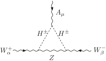
Figure 2: $H^{\pm}W^{\mp}Z$ contribution to the on-shell $W^{\pm}W^{\mp}\gamma$ vertex.

In order to cross–check the above results, $\Delta\kappa$ and $\Delta Q$ were calculated independently by a general method for reducing tensor form factors. This method, which is an extension of the Passarino–Veltman scheme Veltman2 , is described detailed in Ref. Stuart . In such a scheme one assumes that $q^{2}\neq 0$ and applies the usual Passarino–Veltman reduction. The reason why one cannot put $q^{2}=0$ in Eq. (6) prior to applying the tensor reduction is that it would require the inversion of a kinematic matrix whose determinant is $\|{\mathbf{\cal D}}\|=4\,q^{2}\left(m^{2}_{W}-q^{2}\right)$, which evidently vanishes for $q^{2}=0$. Once the form factors for arbitrary $q^{2}$ are obtained, the limit $q^{2}\to 0$ is taken in order to yield the static quantities of the $W$ boson in terms of two–point Passarino-Veltman scalar functions $B_{0}$. Although the limiting procedure $q^{2}\to 0$ involves some additional complications since the application of L’Hôpital rule is required, one important advantage of this method is that it can be computer programmed, thereby eliminating the possibility of any mistake. After this scheme is applied, one is left with the following results:

$$\frac{\Delta\kappa}{a\,s^{2}_{H}} = \frac{1}{2}-\frac{3}{2}\,x_{z}^{2}\,\left(9+2\,x_{z}^{2}\right)+\frac{3}{2}\,x_{h}^{2}\left(1+4\,x_{h}^{2}-2\,x_{h}^{2}\right)+\frac{24\,x_{z}^{2}}{\delta^{2}(x_{h},x_{z})}\,\left(1-x_{z}^{2}-x_{h}^{2}\right)+\frac{3\,x_{h}^{2}}{\delta^{2}(x_{h},x_{z})}{\left(1+x_{z}^{2}-x_{h}^{2}\right)}^{3}\,\Delta B_{1}$$ (19)

$$- 3\,x_{z}^{2}\,\left(x_{z}^{2}-x_{h}^{2}-\frac{4\,x_{z}^{2}}{\delta^{2}(x_{h},x_{z})}\,\left(1-x_{z}^{2}+x_{h}^{2}\right)\right)\,\Delta B_{2},$$

$$\frac{\Delta Q}{a\,s^{2}_{H}} = -\frac{2}{3}+x_{z}^{2}\left(3+2\,x_{z}^{2}\right)-x_{h}^{2}\left(1+4\,x_{z}^{2}-2\,x_{h}^{2}\right)-\frac{4\,x_{z}^{2}}{\delta^{2}(x_{h},x_{z})}\,\left(1-x_{z}^{2}-x_{h}^{2}\right)$$ (20)

$$- \frac{2\,x_{h}^{2}}{\delta^{2}(x_{h},x_{z})}\,\left(x_{z}^{6}+{\left(1-x_{h}^{2}\right)}^{3}-3\,\left(1-x_{h}^{2}+x_{z}^{2}\right)\,x_{z}^{2}\,x_{h}^{2}\right)\,{\Delta B_{1}}$$

$$+ \frac{2\,x_{z}^{2}}{\delta^{2}(x_{h},x_{z})}\,\left(\left(x_{h}^{2}-x_{z}^{2}\right)\,\left(\left(1-x_{z}^{2}+x_{h}^{2}\right)\,x_{z}^{2}+x_{h}^{2}\left(2+x_{z}^{2}-x_{h}^{2}\right)\right)-x_{h}^{2}\right)\,{\Delta B_{2}}.$$

with $\Delta B_{1}=B_{0}(m_{W}^{2},m_{H^{\pm}}^{2},m_{Z}^{2})-B_{0}(0,m_{H^{\pm}}^{2},m_{H^{\pm}}^{2})$ and $\Delta B_{2}=B_{0}(m_{W}^{2},m_{H^{\pm}}^{2},m_{Z}^{2})-B_{0}(0,m_{Z}^{2},m_{Z}^{2})$. These scalar integrals can be solved analytically or numerically evaluated FF . We compared numerically the latter results with those obtained from Eqs. (9)–(10) and observed a perfect agreement. In this way we make sure that our results are correct.

III Discussion

The behavior of $\Delta\kappa/(a\,s^{2}_{h})$ and $\Delta Q(a\,s^{2}_{H})$ as a function of $x_{h}$ is shown in Figs. 3 and 4, respectively. From these figures we can observe that $\Delta\kappa$ is of the order of $a\,s^{2}_{H}$ in the range $2\,m_{W}<m_{H^{\pm}}<10\,m_{W}$, whereas $\Delta Q$ is one order of magnitude below. One can also observe that $\Delta Q$ decreases more rapidly than $\Delta\kappa$ with increasing $m_{H^{\pm}}$. It is convenient to compare our results with those arising from other couplings involving Higgs bosons. For instance, the contribution from the SM $W^{\pm}W^{\mp}H^{0}$ vertex was calculated in Ref. Bardeen , in which case $\Delta\kappa\sim a$ and $\Delta Q\sim 10^{-2}a$ for values of $m_{H}$ in the same range considered for $m_{H^{\pm}}$ in Figs. 3 and 4. Similar results were found in Ref. THDM for the contributions coming from the THDM couplings $W^{\pm}W^{\mp}\phi^{0}$ and $H^{\pm}W^{\mp}\phi^{0}$, with $\phi^{0}=H^{0},\,h^{0}$, and $A^{0}$. We conclude thus that the contribution of the $H^{\pm}W^{\mp}Z$ vertex to $\Delta\kappa$ and $\Delta Q$ may be as important as those contributions arising from other Higgs boson couplings provided that $s_{H}\sim 1$, i.e, when the SSB of the electroweak sector is dictated by the Higgs triplets.

We now would like to focus on the decoupling nature of the Higgs boson contributions to the $\Delta Q$ and $\Delta\kappa$ form factors. The sensitivity of $\Delta\kappa$ to heavy physics effects as well as the decoupling nature of $\Delta Q$ was analyzed in a more general context in Ref. Inami . From Figs. 3 and 4 we can see that $\Delta Q$ decouples for a large Higgs scalar mass, whereas $\Delta\kappa$ does not. These results do not contradict the decoupling theorem, which establishes that those Lorentz structures arising from renormalizable operators can be sensitive to nondecoupling effects, whereas those structures coming from nonrenormalizable operators are suppressed by inverse powers of the heavy mass, thereby decoupling in the large mass limit. As far as $\Delta Q$ and $\Delta\kappa$ are concerned, the former always decouples for a large mass of a particle running in the loop since its Lorentz structure is generated by a nonrenormalizable dimension–six operator; on the contrary, $\Delta\kappa$ may be sensitive to nondecoupling effects as the Lorentz structure associated with this quantity is induced by a renormalizable dimension–four operator. In this context, the decoupling properties of $\Delta Q$ and $\Delta\kappa$ have been discussed in the context of all of the renormalizable theories considered up to now in the literature Bardeen ; TT . For instance, in the SM the heavy Higgs mass limit yields $\Delta Q\to 0$ and $\Delta\kappa\to a$ Bardeen . As far as the THDM is concerned, $\Delta\kappa\to 2\,a$ and $\Delta Q\to 0$ when $m_{\phi^{0}}$ becomes very large and $m_{H^{\pm}}$ is kept fixed, whereas $\Delta\kappa\to-a$ and $\Delta Q\to 0$ in the opposite scenario THDM . In addition, in the same model, both $\Delta\kappa$ and $\Delta Q$ vanish when both $m_{\phi^{0}}$ and $m_{H^{\pm}}$ are very large. In our case, we obtain that $\Delta\kappa\to-(a\,s_{H}^{2})/2$ and $\Delta Q\to 0$ in the heavy charged scalar mass limit. These values follow readily from Eq. (7).

It is interesting to note that our results can also be used to obtain the contribution to the static quantities of the $W$ boson from the $H^{\mp}W^{\pm}Z^{\prime}$ coupling, with $Z^{\prime}$ the extra neutral gauge boson appearing in theories with an extra $U(1)$. This contribution has yet been calculated in the context of an extra $U(1)$ superstring inspired theory Sharma . According to these authors, their results were obtained in the Landau gauge. We have compared numerically our results with those presented Eqs. (12) and (13) of Ref. Sharma and found no agreement. As pointed out above, our results were cross–checked by making a comparison between the results obtained via the Feynman parameters technique and those obtained by the slightly modified version of the Passarino–Veltman scheme described in Refs. TT ; Stuart . These two methods are independent and allows us to make sure that our results are correct.

Figure 3: $\frac{\Delta\kappa}{a\,s^{2}_{H}}$ as a function of $x_{h}=\frac{m_{H^{\pm}}}{m_{W}}$.

Figure 4: $\frac{\Delta Q}{a\,s^{2}_{H}}$ as a function of $x_{h}=\frac{m_{H^{\pm}}}{m_{W}}$.

IV Conclusion

The novel feature of a Higgs–triplet representation is the presence of a tree–level $H^{\pm}W^{\mp}Z$ vertex, whose strength may be of the order of the unity provided that the SSB of the electroweak sector is dictated by the VEV of the neutral components of the Higgs triplet. This class of models can be viable as long as a tree–level custodial $SU(2)$ symmetry is respected by the Higgs potential. The phenomenology of the $H^{\pm}W^{\mp}Z$ coupling is thus be very appealing. Any direct or indirect evidence of the this coupling would be a clear signal of the existence of a scalar sector comprised by Higgs triplets. We have studied the impact of this vertex on the static electromagnetic properties of the $W$ gauge boson. We found that the respective contributions to the form factors $\Delta\kappa$ and $\Delta Q$ are as important as those predicted by the SM coupling $W^{\pm}W^{\mp}H^{0}$ or those arising from the THDM couplings $W^{\pm}W^{\mp}\phi^{0}$ and $H^{\pm}W^{\mp}\phi^{0}$.

We would like to point out that our results can also be used to evaluate the contributions from the $H^{\pm}W^{\mp}Z^{\prime}$ vertex to the magnetic moments of the $W$ boson, where $Z^{\prime}$ is the neutral boson which appears in theories with an extra $U(1)$ gauge symmetry. We note that our results, (9) and (10), disagree with those presented in Ref. Sharma for the contribution from the $H^{\pm}W^{\mp}Z^{\prime}$ coupling in an extra $U(1)$ superstring inspired theory. Finally, We emphasize that our results were cross–checked by making a comparison between the results obtained via the Feynman parameters technique and those obtained by the slightly modified version of the Passarino–Veltman scheme described in Ref. Stuart .

References

• (1) For recent studies on the experimental sensitivity to trilinear gauge boson coupligs see for instance M. Diehl, O. Nachtmann, and F. Nagel, Eur. Phys. J. C 27, 375 (2003); arXiv:hep-ph/0306247.
• (2) W. A. Bardeen, R. Gastmans, and B. Lautrup, Nucl. Phys. B46, 319 (1972).
• (3) G. Couture and J. N. Ng, Z. Phys. C 35, 65 (1987).
• (4) G. Couture, J. N. Ng, J. L. Hewett, and T. G. Rizzo, Phys. Rev. D 36, 859 (1987).
• (5) C. L. Bilachak, R. Gastmans, and A. van Proeyen, Nucl. Phys. B273, 46 (1986); G. Couture, J. N. Ng, J. L. Hewett, and T. G. Rizzo, Phys. Rev. D 38, 860 (1988); A. B. Lahanas and V. C. Spanos, Phys. Lett. B 334, 378 (1994); T. M. Aliyev, ibid. 376, 127 (1996).
• (6) F. Larios, J. A. Leyva, and R. Martínez, Phys. Rev. D 53, 6686 (1996).
• (7) G. Tavares–Velasco and J. J. Toscano, Phys. Rev. D bf 65, 013005-1 (2001).
• (8) T. G. Rizzo and M. A. Samuel, Phys. Rev. D 35, 403 (1987); A. J. Davies, G. C. Joshi, and R. R. Volkas, ibid. 42, 3226 (1990).
• (9) N. K. Sharma, P. Saxena, Sardar Singh, A. K. Nagawat, and R. S. Sahu, Phys. Rev. D 56, 4152 (1997).
• (10) For a review, see J. Ellison and J. Wudka, Annu. Rev. Nucl. Part. Sci. 48, 33 (1998), and references therein.
• (11) J. Gunion, G. Kane, and J. Wudka, Nucl. Phys. B299, 231 (1988); A. Méndez and A. Pomarol, Nucl. Phys. B349, 369 (1991); M. C. Peyranere, H. E. Haber, and P. Irulegui, Phys. Rev. D 44, 191 (1991); S. Kanemura, Phys. Rev. D 61, 095001 (2000); J. L. Díaz–Cruz, J. Hernández-Sánchez, and J. J. Toscano, Phys. Lett. B512, 339 (2001).
• (12) J. Gunion, H. E. Haber, G. Kane, and S. Dawson, The Higgs Hunter’s Guide, Addision–Wesley Publishing Company (1990).
• (13) J. A. Grifols and A. Méndez, Phys. Rev. D 22, 1725 (1980).
• (14) H. Georgi and M. Machacek, Nucl. Phys. B262, 463 (1986); R. S. Chivukula and G. Georgi, Phys. Lett. B182, 181 (1985).
• (15) M. S. Chanowitz and M. Golden, Phys. Lett. B165, 105 (1985).
• (16) J. F. Gunion, R. Vega, and J. Wudka, Phys. Rev. D 42, 1673 (1990).
• (17) K. Cheung, R. Phillips, and A. Pilaftsis, Phys. Rev. D 51, 4731 (1995); R. M. Godbole, B. Mukhopadhyaya, and M. Nowakowski, Phys. Lett. B352, 388 (1995); D. K. Ghosh, R. M. Godbole, and B. Mukhopadhyaya, Phys. Rev. D 55, 3150 (1997).
• (18) K. Cheung and D. K. Ghosh, JHEP 0211, 48 (2002).
• (19) G. Passarino and M. Veltman, Nucl. Phys. B160, 151 (1979)
• (20) See for instance G. Devaraj and R. G. Stuart, Nucl. Phys. B519, 483 (1998).
• (21) G. J. van Oldenborgh, Comput. Phys. Commun. 66 1 (1991); T. Hahn and M. Pérez-Victoria, hep-ph/9807565.
• (22) T. Inami, C. S. Lim, B. Takeuchi, and M. Tanabashi, Phys. Lett. B 381, 458 (1996).