Analysis of Supersymmetric Effects on $B\to\phi K$ Decays
in the PQCD Approach

Abstract

We study the effects of the MSSM contribution on $B\to\phi K$ decays using the perturbative QCD approach. In this approach, strong phases can be calculated, so that we can predict the values of CP asymmetries with the MSSM contribution. We predict a large relative strong phase between the penguin amplitude and the chromomagnetic penguin amplitude. If there is a new CP violating phase in the chromomagnetic penguin amplitude, then the CP asymmetries may change significantly from the SM prediction. We parametrize the new physics contributions that appear in the Wilson coefficients. We maximize the new physics parameters up to the point where it is limited by experimental constraints. In the case of the $LR$ insertion, we find that the direct CP asymmetries can reach about $85\%$ and the indirect CP asymmetry can reach about $-30\%$.

I Introduction

$B\to\phi K_{S}$ decay may be useful in the search for new physics beyond the standard model (SM). The time-dependent CP asymmetry of $B^{0}$ decay into CP eigenstates $f_{CP}$ can be written as $a_{f_{CP}}(t)=A_{f_{CP}}\cos(\Delta M_{B}t)+S_{f_{CP}}\sin(\Delta M_{B}t)$, where $A_{f_{CP}}$ and $S_{f_{CP}}$ characterize direct CP violation and indirect CP violation, respectively. In the SM, both $A_{J/\psi K_{S}}$ and $A_{\phi K_{S}}$ vanish, and both $S_{J/\psi K_{S}}$ and $S_{\phi K_{S}}$ must equal to $\sin(2\phi_{1})$. Any difference between $S_{J/\psi K_{S}}$ and $S_{\phi K_{S}}$ larger than $O(1\%)$ would be a signal for physics beyond the SM Grossman:1996ke . The $B\to\phi K_{S}$ decay amplitude is induced only at the one-loop level, so that new physics might contribute to this decay through quantum effects. At present, BaBar and Belle collaborations have the following results Aubert:2002ic ; Abe:2003yu :

$$S_{J/\psi K_{S}}=\left\{\begin{array}[]{cl}0.741\pm 0.067\pm 0.034&(\mathrm{BaBar,\ 81\,fb}^{-1})\;,\\ 0.733\pm 0.057\pm 0.028&(\mathrm{Belle,\ 140\,fb}^{-1})\;,\\ \end{array}\right.$$ (3)

with $A_{J/\psi K_{S}}=0$. In the $\phi K_{S}$ mode, they have reported the following results Browder:lp2003 ; Abe:2003yt :

$$A_{\phi K_{S}} = \left\{\begin{array}[]{cl}0.38\pm 0.37\pm 0.12&\mathrm{(BaBar,\ 110\,fb}^{-1})\;,\\ -0.15\pm 0.29\pm 0.07&\mathrm{(Belle,\ 140\,fb}^{-1})\;.\\ \end{array}\right.$$ (6)

$$S_{\phi K_{S}} = \left\{\begin{array}[]{cl}0.45\pm 0.43\pm 0.07&\mathrm{(BaBar,\ 110\,fb}^{-1})\;,\\ -0.96\pm 0.50\ {}^{+0.09}_{-0.11}&\mathrm{(Belle,\ 140\,fb}^{-1})\;.\\ \end{array}\right.$$ (9)

Belle collaboration found a $3.5\sigma$ deviation from the SM prediction. In contrast with Belle, the BaBar result is consistent with the SM. If the Belle result continues to hold, and both experiments agree, then their result is a signal for new physics. There have been many papers which studied new physics contributions to $B\to\phi K_{S}$ decay amplitude. Some authors Lunghi:2001af ; Silvestrini:2002sm ; Kane:2002sp analyzed the supersymmetric contribution using the mass insertion approximation, which is a powerful tool for model-independent analysis of new physics associated with the minimal supersymmetric standard model (MSSM) Hall:1985dx . The new physics contributions come into the Wilson coefficients, which can be calculated perturbatively Gabbiani:1996hi . The problem is how to calculate the decay amplitudes with nonperturbative contributions. To calculate the decay amplitudes, some authors used naive factorization Wirbel:1985ji , generalized factorization Ali:1997nh , or QCD factorization Beneke:1999br . Each method is plagued with large theoretical uncertainties. There are other approaches for this calculation, one of them is the perturbative QCD (PQCD) approach Keum:2000ph . In this paper, we use the PQCD approach and the mass insertion approximation for an estimation of the MSSM contribution in $B\to\phi K$ decays.

The PQCD approach for exclusive $B$ meson decays is based on the $k_{T}$ factorization theorem, in which the decay amplitudes can be separated into perturbative and non-perturbative parts Li:2000hh . The non-perturbative parts are factorized into meson wave functions, which are derived from the other methods, for example, the light-cone QCD sum rules Ball:1998tj ; Ball:1998sk ; Ball:2003sc . A strong phase, which comes from physical intermediate states, is calculable in the PQCD approach. A large strong phase is induced from an annihilation diagram such as Fig. 1(a) Keum:2000ph .

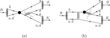
Figure 1: These diagrams generate a large strong phase in the PQCD approach. The dashed lines denote the physical intermediate states.

The strong phase mainly comes from the cut on the virtual gluon line. The source of the strong phase is one of the important differences between the PQCD approach and other methods. PQCD has been applied to some hadronic two-body $B$ meson decays at leading order in $\alpha_{s}$, and the results are consistent with experimental data except for $\eta^{(\prime)}K$ and $\pi^{0}\pi^{0}$ Keum:2000ph ; Lu:2000em . $B\to\phi K$ decays were also calculated using the PQCD approach in Refs. Mishima:2001pp ; Chen:2001pr .

Another important difference between PQCD and other methods is how to calculate magnetic penguin diagrams that are induced from the chromomagnetic penguin operator $O_{8G}$. In many models, the chromomagnetic penguin amplitude is most sensitive to new physics Keum:1999vt ; Moroi:2000tk . However, it is difficult to calculate the chromomagnetic penguin in naive factorization and generalized factorization, because we do not know the magnitude of $q^{2}$, which is the momentum transferred by the gluon in the chromomagnetic penguin operator. Therefore, proponents of these factorization approach treat $q^{2}$ as an input parameter, so that the result is directly proportional to the assumed values for $\langle 1/q^{2}\rangle$ Ali:1997nh . In the PQCD and QCD factorization approaches, the chromomagnetic penguin amplitudes can be calculated without any assumption for the value of $q^{2}$. We studied the chromomagnetic penguin using the PQCD approach in Ref. Mishima:2003wm , and we found that the chromomagnetic penguin generated a strong phase from the diagram as Fig. 1(b). In the PQCD approach, $q^{2}$ is written as $(1-x_{2})x_{3}M_{B}^{2}-|\mbox{\boldmath{$k$}}_{2T}-\mbox{\boldmath{$k$}}_{3T}|^{2}$. Here, $x_{2}$ and $x_{3}$ are momentum fractions of partons in $K$ and $\phi$ mesons, respectively. $\mbox{\boldmath{$k$}}_{2T}$ and $\mbox{\boldmath{$k$}}_{3T}$ are transverse momenta of the partons. In QCD factorization, $q^{2}$ can be written in terms of the momentum fraction of partons too, however, they expand the amplitude in power of $|\mbox{\boldmath{$k$}}_{2T}-\mbox{\boldmath{$k$}}_{3T}|^{2}/[(1-x_{2})x_{3}M_{B}^{2}]$ and for the leading order they have $q^{2}=(1-x_{2})x_{3}M_{B}^{2}$. In this expansion, $q^{2}$ never vanishes. There is no absorptive part in the amplitude and the strong phase is not generated from the chromomagnetic penguin. The fact that we get large imaginary part implies that this expansion is not valid.

The outline of this paper is as follows. First, we consider the MSSM contribution in the effective Hamiltonian for $B$ meson decays. We present the Wilson coefficients with the MSSM using the mass insertion approximation. Next, we briefly review the PQCD approach for the exclusive $B$ meson decays. We show the result at the leading order in $\alpha_{s}$ and how to calculate the chromomagnetic penguin amplitudes. Furthermore, we calculate the MSSM contribution in $B\to\phi K$ decays with the $LR$, $RL$, $LL$, and $RR$ insertions. We consider the both $B^{0}\to\phi K_{S}$ and $B^{\pm}\to\phi K^{\pm}$ modes, and calculate the branching ratios, the direct CP asymmetries, and the indirect CP asymmetry. Finally, we summarize this study.

II MSSM Contributions in $B\to\phi K$ Decays

II.1 Effective Hamiltonian for $B$ Meson Decays

We use the effective Hamiltonian in the calculation of $B$ meson decays Buchalla:1995vs . The Hamiltonian is expressed as the convolution of local operators and the Wilson coefficients. The effective Hamiltonian with a $b\to s$ transition is given by

$$H_{\rm eff} = \frac{G_{F}}{\sqrt{2}}\left[\sum_{q^{\prime}=u,c}V_{q^{\prime}s}^{*}V_{q^{\prime}b}\left(C_{1}(\mu)O_{1}^{(q^{\prime})}(\mu)+C_{2}(\mu)O_{2}^{(q^{\prime})}(\mu)\right)\right.$$ (10)

$$\left.-V_{ts}^{*}V_{tb}\left(\sum_{i=3}^{10}C_{i}(\mu)O_{i}(\mu)+C_{7\gamma}(\mu)O_{7\gamma}(\mu)+C_{8G}(\mu)O_{8G}(\mu)\right)\right]+{\rm H.c.}\;,$$

where $V_{q^{\prime}s}^{*}$ and $V_{q^{\prime}b}$ are the Cabibbo-Kobayashi-Maskawa matrix elements Cabibbo:yz . $O_{1-10}$ are local four-fermi operators, $O_{7\gamma}$ is the photomagnetic penguin operator, and $O_{8G}$ is the chromomagnetic penguin operator. The local operators are given by

$$O_{1}^{(q^{\prime})}=(\bar{s}_{i}q^{\prime}_{j})_{V-A}(\bar{q^{\prime}}_{j}b_{i})_{V-A}\;,\;\;\;\;\;\;\;\;O_{2}^{(q^{\prime})}=(\bar{s}_{i}q^{\prime}_{i})_{V-A}(\bar{q^{\prime}}_{j}b_{j})_{V-A}\;,$$

$$O_{3}=(\bar{s}_{i}b_{i})_{V-A}\sum_{q}(\bar{q}_{j}q_{j})_{V-A}\;,\;\;\;\;\;\;\;O_{4}=(\bar{s}_{i}b_{j})_{V-A}\sum_{q}(\bar{q}_{j}q_{i})_{V-A}\;,$$

$$O_{5}=(\bar{s}_{i}b_{i})_{V-A}\sum_{q}(\bar{q}_{j}q_{j})_{V+A}\;,\;\;\;\;\;\;\;O_{6}=(\bar{s}_{i}b_{j})_{V-A}\sum_{q}(\bar{q}_{j}q_{i})_{V+A}\;,$$

$$O_{7}=\frac{3}{2}(\bar{s}_{i}b_{i})_{V-A}\sum_{q}e_{q}(\bar{q}_{j}q_{j})_{V+A}\;,\;O_{8}=\frac{3}{2}(\bar{s}_{i}b_{j})_{V-A}\sum_{q}e_{q}(\bar{q}_{j}q_{i})_{V+A}\;,$$

$$O_{9}=\frac{3}{2}(\bar{s}_{i}b_{i})_{V-A}\sum_{q}e_{q}(\bar{q}_{j}q_{j})_{V-A}\;,\;O_{10}=\frac{3}{2}(\bar{s}_{i}b_{j})_{V-A}\sum_{q}e_{q}(\bar{q}_{j}q_{i})_{V-A}\;,$$

$$O_{7\gamma}=\frac{e}{8\pi^{2}}m_{b}\bar{s}_{i}\sigma^{\mu\nu}(1+\gamma_{5})b_{i}F_{\mu\nu}\;,\;\;O_{8G}=-\frac{g_{s}}{8\pi^{2}}m_{b}\bar{s}_{i}\sigma^{\mu\nu}(1+\gamma_{5})T^{a}_{ij}b_{j}G^{a}_{\mu\nu}\;.$$ (11)

Here, $i$ and $j$ are color indices, $q$ is taken to be $u,\;d,\;s$, and $c$, and $(\bar{q}q)_{V\pm A}=\bar{q}\gamma_{\mu}(1\pm\gamma_{5})q$. We define the covariant derivative as $D_{\mu}=\partial_{\mu}+ig_{s}T^{a}A^{a}_{\mu}-ieA_{\mu}$, so that the signs of the magnetic penguin operators are different between $O_{7\gamma}$ and $O_{8G}$. We integrate out the degree of freedom of high energy particles, then the Wilson coefficients include high energy information. If we consider the new physics effect on $B$ decays, then we need to calculate the Wilson coefficients with new physics contributions.

II.2 MSSM Contribution and Mass Insertion Approximation

We consider the MSSM contribution for $B\to\phi K$ decays. Generally, there are new sources of the CP violation and the flavor changing neutral current (FCNC) in the MSSM, so that there may be direct CP violations, and it is possible that $S_{\phi K_{S}}$ becomes different from $S_{J/\psi K_{S}}$. Since we do not want our computation to depend on specific SUSY models, we use the mass insertion approximation to calculate the Wilson coefficients with the MSSM. In the mass insertion approximation, the FCNC effect appears in the squark propagators through the off-diagonal elements in the squark mass matrices. The decay amplitudes are expanded in terms of $(\delta^{d})_{ij}=(V_{d}^{\dagger}m^{2}_{\tilde{d}}V_{d})_{ij}/m^{2}_{\tilde{q}}$, where $m_{\tilde{d}}^{2}$ is the squared down-type squark mass matrix, $m_{\tilde{q}}$ is an average squark mass, and $V_{d}$ is the matrix which diagonalizes the down-type quark mass matrix. Of course, we must consider the region of $|(\delta^{d})_{ij}|<1$. For example, a transition of a right-handed fermion to a left-handed fermion is parameterized by $(\delta^{d}_{LR})_{ij}$. There are four mass insertions: $(\delta^{d}_{LL})_{ij}$, $(\delta^{d}_{RR})_{ij}$, $(\delta^{d}_{LR})_{ij}$, and $(\delta^{d}_{RL})_{ij}$. The $b\to s$ transition is induced from the gluino-squark loop, the chargino-squark loop, and the neutralino-squark loop. In this study, we consider only the gluino contribution, which is dominant in many models. The Wilson coefficients for penguin and magnetic penguin are given by

$$C_{3}^{\rm NP}(M_{S}) \simeq -\frac{\sqrt{2}\alpha_{s}^{2}}{4G_{F}V_{ts}^{*}V_{tb}m_{\tilde{q}}^{2}}(\delta_{LL}^{d})_{23}\left[-\frac{1}{9}B_{1}(x)-\frac{5}{9}B_{2}(x)-\frac{1}{18}P_{1}(x)-\frac{1}{2}P_{2}(x)\right]\;,$$

$$C_{4}^{\rm NP}(M_{S}) \simeq -\frac{\sqrt{2}\alpha_{s}^{2}}{4G_{F}V_{ts}^{*}V_{tb}m_{\tilde{q}}^{2}}(\delta_{LL}^{d})_{23}\left[-\frac{7}{3}B_{1}(x)+\frac{1}{3}B_{2}(x)+\frac{1}{6}P_{1}(x)+\frac{3}{2}P_{2}(x)\right]\;,$$

$$C_{5}^{\rm NP}(M_{S}) \simeq -\frac{\sqrt{2}\alpha_{s}^{2}}{4G_{F}V_{ts}^{*}V_{tb}m_{\tilde{q}}^{2}}(\delta_{LL}^{d})_{23}\left[\frac{10}{9}B_{1}(x)+\frac{1}{18}B_{2}(x)-\frac{1}{18}P_{1}(x)-\frac{1}{2}P_{2}(x)\right]\;,$$

$$C_{6}^{\rm NP}(M_{S}) \simeq -\frac{\sqrt{2}\alpha_{s}^{2}}{4G_{F}V_{ts}^{*}V_{tb}m_{\tilde{q}}^{2}}(\delta_{LL}^{d})_{23}\left[-\frac{2}{3}B_{1}(x)+\frac{7}{6}B_{2}(x)+\frac{1}{6}P_{1}(x)+\frac{3}{2}P_{2}(x)\right]\;,$$

$$C_{7\gamma}^{\rm NP}(M_{S}) \simeq \frac{\sqrt{2}\alpha_{s}\pi}{6G_{F}V_{ts}^{*}V_{tb}m_{\tilde{q}}^{2}}\left[(\delta_{LL}^{d})_{23}\frac{8}{3}M_{3}(x)+(\delta_{LR}^{d})_{23}\frac{m_{\tilde{g}}}{m_{b}}\frac{8}{3}M_{1}(x)\right]\;,$$

$$C_{8G}^{\rm NP}(M_{S}) \simeq \frac{\sqrt{2}\alpha_{s}\pi}{2G_{F}V_{ts}^{*}V_{tb}m_{\tilde{q}}^{2}}\left[(\delta_{LL}^{d})_{23}\left(\frac{1}{3}M_{3}(x)+\!3M_{4}(x)\right)\right.$$ (12)

$$\left.\ \ \ \ \ \ \ \ \ \ \ \ \ \ \ \ \ \ \ +(\delta_{LR}^{d})_{23}\frac{m_{\tilde{g}}}{m_{b}}\left(\frac{1}{3}M_{1}(x)+3M_{2}(x)\right)\right]\;,$$

at the first order in the mass insertion approximation Gabbiani:1996hi . Here, $M_{S}$ is the SUSY scale, and $x=m^{2}_{\tilde{g}}/m^{2}_{\tilde{q}}$, where $m_{\tilde{g}}$ is the gluino mass. $B(x)$, $P(x)$ and $M(x)$ are the loop functions, which are calculated from box diagrams and penguin diagrams Gabbiani:1996hi ; Harnik:2002vs . New physics contributions induce additional operators, which are obtained from Eq. (11) by exchanging $L$ and $R$. The penguin coefficients $C_{3}^{\rm NP}(M_{S})-C_{6}^{\rm NP}(M_{S})$ depend only on $\delta^{d}_{LL}$, and the magnetic-penguin coefficients $C_{7\gamma}^{\rm NP}(M_{S})$ and $C_{8G}^{\rm NP}(M_{S})$ depend on both $\delta^{d}_{LL}$ and $\delta^{d}_{LR}$. It is noted that the $\delta^{d}_{LR}$ terms have a chiral enhancement factor $m_{\tilde{g}}/m_{b}$. This factor is important when we constraint the parameters from the branching ratio for $B\to X_{s}\gamma$, as we will return it on later.

III $B\to\phi K$ Decays in PQCD Approach

Let us briefly review the PQCD approach for exclusive $B$ meson decays. The PQCD formalism is based on the factorization of decay amplitudes into a product of long-distant physics, which is identified with meson wave functions, and short-distant physics Lepage:1979zb . The meson distribution amplitudes are universal in the processes under consideration, and they are determined from experiments and/or other theoretical methods: the light-cone QCD sum rules, lattice calculations, etc. Process dependence is exhibited in the short-distant part. For example, let us consider $B\to\phi K$. Figure. 2 shows the PQCD quark-level diagram for this decay. At the black blob, the decay $\bar{b}\to\bar{s}s\bar{s}$ takes place. The $s\bar{s}$ pair forms a $\phi$ meson. The other $s$ quark recoils against the $\phi$ meson carrying almost $m_{b}/2$ momentum. In order for the spectator quark to form a $K$ meson together with the fast moving $s$ quark, it has to exchange a gluon in order to change its momentum from $k_{1}$ to $k_{2}$.

We consider the $B\to\phi K$ decays.

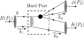
Figure 2: A leading-order diagram in $B\to\phi K$.

In the light-cone coordinates, the $B$ meson momentum $P_{1}$, the $K$ meson momentum $P_{2}$, and the $\phi$ meson momentum $P_{3}$ are taken to be

$$P_{1}=\frac{M_{B}}{{\sqrt{2}}}(1,1,\mbox{\boldmath{$0$}}_{T})\;,\;\;P_{2}=\frac{M_{B}}{{\sqrt{2}}}(1-r_{\phi}^{2},0,\mbox{\boldmath{$0$}}_{T})\;,\;\;P_{3}=\frac{M_{B}}{{\sqrt{2}}}(r_{\phi}^{2},1,\mbox{\boldmath{$0$}}_{T})\;,$$ (13)

where $r_{\phi}=M_{\phi}/M_{B}$. Here, we consider the $B$ meson to be at rest, and the $K$ meson mass is ignored. The momenta of partons $k_{1}$, $k_{2}$, and $k_{3}$ defined in Fig. 2 are written as

$$k_{1}=(0,x_{1}P_{1}^{-},\mbox{\boldmath{$k$}}_{1T})\;,\;\;k_{2}=(x_{2}P_{2}^{+},0,\mbox{\boldmath{$k$}}_{2T})\;,\;\;k_{3}=(0,x_{3}P_{3}^{-},\mbox{\boldmath{$k$}}_{3T})\;.$$ (14)

A hard part in Fig. 2 has two propagators:

$$\frac{1}{(k_{1}-k_{2})^{2}}\ \cdot\ \frac{1}{(P_{1}-k_{2})^{2}-M_{B}^{2}} \simeq \frac{1}{-x_{1}x_{2}M_{B}^{2}-|\mbox{\boldmath{$k$}}_{1T}-\mbox{\boldmath{$k$}}_{2T}|^{2}}\ \cdot\ \frac{1}{-x_{2}M_{B}^{2}-|\mbox{\boldmath{$k$}}_{2T}|^{2}}\;.$$ (15)

If we neglect transverse momenta of partons, then a singularity arises from the end-point region of parton momenta since the hard part is proportional to $1/x_{1}x_{2}^{2}$. Therefore, we conclude that the transverse components are present and they cannot be ignored. Retaining $k_{T}$ for partons, large double logarithms appear through radiative corrections. The resummation of those double logarithms leads to the Sudakov factor Botts:kf . The Sudakov factor suppresses the end-point of the parton momentum and the large transverse separation between a quark and an antiquark in mesons. Therefore, it guarantees a perturbative calculation of the hard part Li:1992nu . The other double logarithms appear from the end-point region of the parton momenta. Their resummation, which is the so-called threshold resummation, leads to another factor in the hard part Li:2001ay . This factor also ensures the absence of the end-point singularities in PQCD, and the arbitrary cutoffs used in QCD factorization are not necessary. A typical decay amplitude for $B\to\phi K$ can be expressed as the convolutions of a hard part, meson wave functions, and the Wilson coefficient, in the space of $x_{i}$ and $b_{i}$, where $b_{i}$ is the conjugate variable to $k_{iT}$ Chang:1996dw .

$${\cal M} = \int_{0}^{1}dx_{1}dx_{2}dx_{3}\int_{0}^{\infty}db_{1}db_{2}db_{3}\,\Phi_{K}(x_{2},b_{2})\,e^{-S_{K}(x_{2},b_{2},t)}\,\Phi_{\phi}(x_{3},b_{3})\,e^{-S_{\phi}(x_{3},b_{3},t)}$$ (16)

$$\hskip 48.36967pt\times C\left(t\right)H(x_{1},x_{2},x_{3},b_{1},b_{2},b_{3},t)\,J(x_{1},x_{2},x_{3})\,\Phi_{B}(x_{1},b_{1})\,e^{-S_{B}(x_{1},b_{1},t)}\;.$$

Here, $\Phi_{B}$, $\Phi_{K}$, and $\Phi_{\phi}$ are the meson wave functions, and $H$ is the hard part. $S_{B}$, $S_{K}$, and $S_{\phi}$ denote the Sudakov factors, and $J$ denotes the threshold factor. The scale $t$, which characterizes the hard part, is of order of $\sqrt{\bar{\Lambda}M_{B}}$ where $\bar{\Lambda}=M_{B}-m_{b}$. The formula in Eq. (16) is the typical amplitude for an exclusive $B$ meson decays based on the $k_{T}$ factorization.

III.1 $B\to\phi K$ in the Standard Model

For $B\to\phi K$ decays, we calculate the diagrams shown in Fig. 3 at leading order in the PQCD approach.

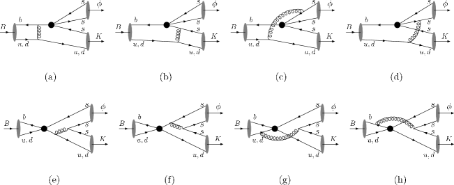
Figure 3: Leading order diagrams for $B\to\phi K$ decays. The ellipses denote the meson wave functions, and the thick points denote the local operators.

The diagrams (a) and (b) are dominant contributions, and the diagrams (e) and (f) generate a large strong phase Keum:2000ph . Except for a small tree diagram contribution in the $B^{\pm}\to\phi K^{\pm}$ decay amplitude, both $B^{0}\to\phi K^{0}$ and $B^{\pm}\to\phi K^{\pm}$ decay amplitudes get contributions from pure penguin graphs. For $B$ meson, we use the model wave function

$$\phi_{B}(x,b) = N_{B}x^{2}(1-x)^{2}\exp\left[-\frac{1}{2}\left(\frac{xM_{B}}{\omega_{B}}\right)^{2}-\frac{\omega_{B}^{2}b^{2}}{2}\right]\;,$$ (17)

where $b$ is the conjugate space of $k_{T}$. $\omega_{B}$ is the shape parameter to be $0.40\pm 0.04$ and $N_{B}$ is the normalization constant Kurimoto:2001zj . For $K$ and $\phi$ mesons, we use the wave functions that were calculated using the light-cone QCD sum rules Ball:1998tj ; Ball:1998sk ; Ball:2003sc . The formulas of the decay amplitudes for $B\to\phi K$ are shown in Ref. Mishima:2001pp . We get the following numerical results within the SM:

$$\mathrm{Br}(B^{0}\to\phi K^{0}) = (8.5{}^{+3.0}_{-2.0}\pm 2.6)\times 10^{-6}\;,$$ (18)

$$\mathrm{Br}(B^{\pm}\to\phi K^{\pm}) = (9.3{}^{+3.1}_{-2.1}\pm 2.8)\times 10^{-6}\;.$$ (19)

The values for various parameters that we use in this calculation are presented in Appendix A. Here, the first error is estimated from the shape parameter $\omega_{B}$ in the $B$ meson wave function, and the second error comes from higher-order contributions. We expect that the higher-order contributions are about $30\%$. The theoretical errors are reduced in CP asymmetries, because errors associated with wave functions cancel out between the denominator and the numerator. The current experimental data are given by Aubert:2003hz ; unknown:2003jf :

$$\mathrm{Br}(B^{0}\to\phi K^{0}) = \left\{\begin{array}[]{cl}(8.4{}^{+1.5}_{-1.3}\pm 0.5)\times 10^{-6}&(\mathrm{BaBar})\;,\\ (9.0{}^{+2.2}_{-1.8}\pm 0.7)\times 10^{-6}&(\mathrm{Belle})\;,\\ \end{array}\right.$$ (22)

$$\mathrm{Br}(B^{\pm}\to\phi K^{\pm}) = \left\{\begin{array}[]{cl}(10.0{}^{+0.9}_{-0.8}\pm 0.5)\times 10^{-6}&(\mathrm{BaBar})\;,\\ (9.4\pm 1.1\pm 0.7)\times 10^{-6}&(\mathrm{Belle})\;.\\ \end{array}\right.$$ (25)

The predicted branching ratios in PQCD are consistent with the experimental data.

III.2 Chromomagnetic Penguin and New Physics

The chromomagnetic penguin operator $O_{8G}$ in Eq. (12) plays an important role in the estimation of new physics contribution. The chromomagnetic penguin diagrams are shown in Fig. 4.

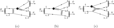
Figure 4: chromomagnetic penguin diagrams in $B\to\phi K$ decays. We show only dominant diagrams in the chromomagnetic penguin amplitude.

We show only dominant diagrams in the chromomagnetic penguin amplitude Mishima:2003wm . Since there must be at least one hard gluon emitted by the spectator quark, the chromomagnetic penguin amplitudes are of next-to-leading order in $\alpha_{s}$ in the PQCD formalism. Obviously, there are many other higher-order diagrams that must be considered simultaneously. Here we limit ourselves to computing only the nonvanishing leading-order terms and leave the higher-order terms for future computation. As we pointed out before new physics contribution comes in through the chromomagnetic penguin in spite of the fact that the leading term is ${\cal O}(\alpha_{s}^{2})$. Of course, regular penguin amplitudes may also contain new physics and they are ${\cal O}(\alpha_{s})$, and we include them. In summary, we calculate the amplitude

$${\cal A}=C^{\rm SM}_{1-10}\otimes H\left(\alpha_{s}\right)\ +\ C^{\rm NP}_{3-6}\otimes H\left(\alpha_{s}\right)\ +\ C^{\rm NP}_{8G}\otimes H\left(\alpha_{s}^{2}\right)\;.$$ (26)

As we will see below that these penguin amplitudes and chromomagnetic penguin amplitudes give comparable contributions.

IV Numerical Analysis

In this section, we estimate the MSSM effect on the branching ratios and the CP asymmetries for both $B^{0}\to\phi K^{0}$ and $B^{\pm}\to\phi K^{\pm}$ decays. We take single mass insertion: one of the $LR$, $RL$, $LL$, and $RR$ insertions, which are parametrized by $\delta_{LR}$, $\delta_{RL}$, $\delta_{LL}$, and $\delta_{RR}$, respectively. First, we constrain them from the branching ratio for $B\to X_{s}\gamma$, which is an inclusive decay mode with the $b\to s$ transition Kagan:1998ym . This mode is theoretically very clean. The theoretical prediction with in the context of the SM agrees with experimental data within errors, so that this mode will give meaningful constraint on any new physics we might introduce. Next, we apply the constrained parameters to $B\to\phi K$ decays. We calculate the branching ratios and the direct and indirect CP asymmetries with the MSSM contribution.

IV.1 Constraint from $B\to X_{s}\gamma$

We constrain the mass insertion parameters from ${\rm Br}(B\to X_{s}\gamma)$. The experimental result is $\mathrm{Br}(B\to X_{s}\gamma)=(3.3\pm 0.4)\times 10^{-4}$ Hagiwara:fs , and we take it with the $2\sigma$ error to constrain the parameters. The results for each insertion are shown in Fig. 5.

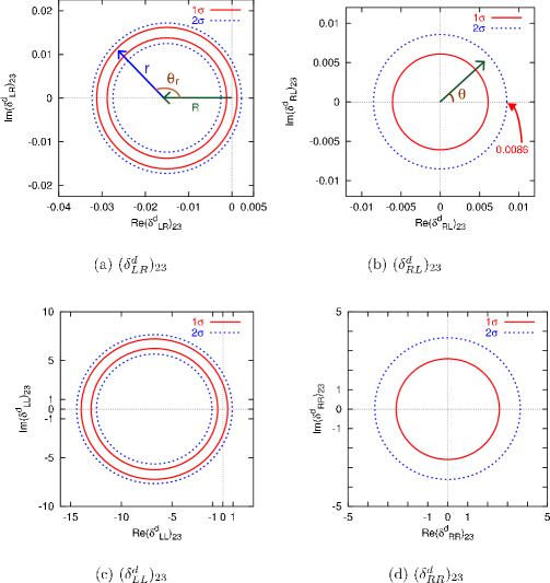
Figure 5: The allowed region for $(\delta^{d}_{LR})_{23}$, $(\delta^{d}_{RL})_{23}$, $(\delta^{d}_{LL})_{23}$, and $(\delta^{d}_{RR})_{23}$ constrained from $\mathrm{Br}(B\to X_{s}\gamma)$. The solid lines denote the region in the $1\sigma$ error, and the dotted lines are the $2\sigma$ error. We take $m_{\tilde{g}}$ and $m_{\tilde{q}}$ to be $500$ GeV. In the analysis of $B\to\phi K$, we take the following parametrization: $(\delta^{d}_{LR})_{23}=R+re^{i\theta_{r}}$ and $(\delta^{d})_{23}=|(\delta^{d})_{23}|e^{i\theta}$ for the $RL$, $LL$, and $RR$ insertions.

In this calculation, we take the gluino mass $m_{\tilde{g}}$ and the squark mass $m_{\tilde{q}}$ to be $500$ GeV. The constraints for $(\delta^{d}_{LR})_{23}$ and $(\delta^{d}_{RL})_{23}$ are strong, while those for $(\delta^{d}_{LL})_{23}$ and $(\delta^{d}_{RR})_{23}$ are very weak. This is because amplitudes with $(\delta^{d}_{LR})_{23}$ and $(\delta^{d}_{RL})_{23}$ are enhanced by a $m_{\tilde{g}}/m_{b}$ factor.

IV.2 $B\to\phi K$ Decays with the MSSM

We calculate the MSSM effect on $B^{0}\to\phi K^{0}$ and $B^{\pm}\to\phi K^{\pm}$ decays with $LR$, $RL$, $LL$, and $RR$ insertions. In the case of the $LR$ insertion, we parametrize $(\delta^{d}_{LR})_{23}$ as

$$(\delta^{d}_{LR})_{23}=R+re^{i\theta_{r}}\;,$$ (27)

where $R$ is a constant, and $r$ and $\theta_{r}$ are parameters as shown in Fig. 5(a). In the SM, $(\delta^{d}_{LR})_{23}$ is equal to $0$, that is, $r=-R$ and $\theta_{r}=0$. Since the constraints for $(\delta^{d}_{LL})_{23}$ and $(\delta^{d}_{RR})_{23}$ from $\mathrm{Br}(B\to X_{s}\gamma)$ are very weak, we take the arbitrary bounds $|(\delta^{d}_{LL})_{23}|<1$ and $|(\delta^{d}_{RR})_{23}|<1$ in order to use the mass insertion approximation. Both the $LL$ and $RR$ insertions have the same contribution to $B\to\phi K$ decays. In the case of the $RL$ and $LL$($RR$) insertions, we use the angle $\theta$ in Fig. 5(b) as a parameter:

$$(\delta^{d})_{23}=|(\delta^{d})_{23}|e^{i\theta}\;.$$ (28)

In the following analysis, we scan all values on the allowed region in Fig. 5(a) for the $LR$ insertion. For the $RL$ and $LL$($RR$) insertions, we take some specific values $|(\delta^{d}_{RL})_{23}|=0.001$ or $0.0086$, and $|(\delta^{d}_{LL(RR)})_{23}|=0.5$ or $1.0$.

The $B_{s}-\overline{B_{s}}$ mixing may also be affected by the MSSM contribution Silvestrini:2002sm , so that we have examined it in order to constraint the mass insertion parameters. The current experimental data is $\Delta M_{s}>14.4\ \mathrm{ps}^{-1}$ (at 95% C.L.) Stocchi:2002yi . The values of $\Delta M_{s}$ is not very sensitive to the presence of the $LR$ and $RL$ insertions. In the case of the $LL$ and $RR$ insertions, their allowed regions are reduced somewhat but these insertions in the $B\to\phi K$ amplitudes is small so that it does not affect our analysis.

Possible MSSM modification for $B\to\phi K$ branching ratios are shown in Fig. 6.

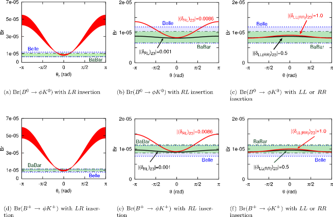
Figure 6: The branching ratios with the MSSM contribution. We take $m_{\tilde{g}}$ and $m_{\tilde{q}}$ to be $500$ GeV. The dot-dashed lines and the dotted lines are the experimental data with the $1\sigma$ error by BaBar and Belle, respectively.

As it can be seen from the figures, the $LR$ insertion may give large effect on the branching ratios for $B\to\phi K$ decays, while the contributions from $RL$ and $LL$($RR$) insertions are small. In the PQCD approach, there are large theoretical uncertainties in the calculation of the branching ratios. Therefore, it is difficult to obtain meaningful constraints from the branching ratios for $B\to\phi K$ decays. In the case of the $LR$ insertion, we suppose $|\theta_{r}|$ is less than $\pi/2$. In the case of the other insertions, we cannot constrain the parameters from the branching ratios.

The results of the direct CP asymmetries are shown in Fig. 7.

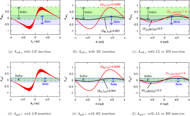
Figure 7: Direct CP asymmetries with the MSSM contribution. We take $m_{\tilde{g}}$ and $m_{\tilde{q}}$ to be $500$ GeV. The dot-dashed lines and the dotted lines are the experimental data with the $1\sigma$ error by BaBar and Belle, respectively.

The experimental data of the direct CP asymmetry for the charged mode are ${\cal A}_{\phi K^{\pm}}=0.04\pm 0.09\pm 0.01$ (BaBar Aubert:2003hz ) and $0.01\pm 0.12\pm 0.05$ (Belle unknown:2003jf ). In the SM, the direct CP asymmetries are almost 0, since $B\to\phi K$ decays are penguin dominant processes. In the case of the $LR$ insertion, the direct CP asymmetries can reach about $85\%$. These asymmetries are generated from the interference between penguin amplitudes in the SM and chromomagnetic penguin amplitudes in the MSSM. Since the relative strong phase between those amplitudes is large, it might be possible to get the large direct CP asymmetries in the PQCD approach. It is noted that the direct CP asymmetry in the neutral mode is almost the same as one in the charged mode. This result from the fact that the chromomagnetic penguin contributions as well as the SM contributions are almost the same in both modes. Since the current experimental data of the direct CP asymmetry in the charged mode is small, we expect that one in the neutral mode will be also small.

Next, we consider the indirect CP asymmetry in $B^{0}\to\phi K_{S}$ decay. The results are shown in Fig. 8.

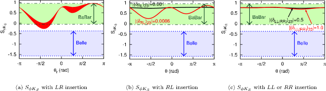
Figure 8: The result of $S_{\phi K_{S}}$ with the MSSM contribution. We take $m_{\tilde{g}}$ and $m_{\tilde{q}}$ to be $500$ GeV. The dot-dashed lines and the dotted lines are the experimental data with the $1\sigma$ error by BaBar and Belle, respectively.

The current BaBar data is consistent with the SM prediction, however, Belle data is not. Our result is $S_{\phi K_{S}}\geq-0.28$ in the $LR$ insertion case. If we change the gluino mass and the squark mass, while the ratio is fixed, then $S_{\phi K_{S}}$ does not change. If we fix the squark mass and take a heavier gluino mass, then $S_{\phi K_{S}}$ becomes larger. If we fix the gluino mass and take a heavier squark mass, then $S_{\phi K_{S}}$ becomes somewhat smaller, that is, new physics contribution becomes larger, and $S_{\phi K_{S}}$ remains almost constant over $m_{\tilde{q}}$ to be a few TeV. Here, we constrained $(\delta^{d}_{LR})_{23}$ from ${\rm Br}(B\to X_{s}\gamma)$, so that if we take a larger $m_{\tilde{q}}$, then $(\delta^{d}_{LR})_{23}$ increases and $C_{8G}^{NP}$ increases slightly. In order to study the effect of the mass on $S_{\phi K_{S}}$, we take an extreme case where the gluino mass is $200$ GeV and the squark mass is $2$ TeV. In this case, $(\delta^{d}_{LR})_{23}$ is still ${\cal O}(10^{-2})$, and the mass insertion approximation can be used. The result is shown in Fig. 9.

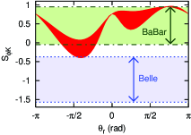
Figure 9: As an example of the extreme case, we take $m_{\tilde{g}}$ to be $200$ GeV and $m_{\tilde{q}}$ to be $2$ TeV in the case of the $LR$ insertion. The dot-dashed lines and the dotted lines are the experimental data with the $1\sigma$ error by BaBar and Belle, respectively.

Even in this case, the $S_{\phi K_{S}}$ can only reach about $-40\%$. Therefore, it is difficult to explain the current Belle data by the new physics we considered here.

Finally, we comment one of the differences between our results and that of QCD factorization. A negative $S_{\phi K_{S}}$ in Fig. 8(a) implies a negative $A_{\phi K_{S}}$ in Fig. 7(a). In an analysis using QCD factorization, a negative $S_{\phi K_{S}}$ implies that $A_{\phi K_{S}}(=-C_{\phi K_{S}})$ is positive in contrast to our results Kane:2002sp . It is caused by the difference in the origin of the strong phase in PQCD and QCD factorization.

V Conclusion

$B\to\phi K$ is one of the most important decay modes in the search for new physics. In this paper, we estimated MSSM contribution in the $B\to\phi K$ decays using the PQCD approach. In PQCD, strong phases are calculable, and we can predict CP asymmetries. We considered the single mass insertions $(\delta_{LR}^{d})_{23}$, $(\delta_{RL}^{d})_{23}$, $(\delta_{LL}^{d})_{23}$, and $(\delta_{RR}^{d})_{23}$, and constrain them from ${\rm Br}(B\to X_{s}\gamma)$. We found that the $LR$ insertion may change the branching ratios and the CP asymmetries in $B\to\phi K$ significantly. The effect of the $RL$ insertion is somewhat smaller than the $LR$ insertion, and that of the $LL$ and $RR$ insertions is little.

In the case of the $LR$ insertion, $A_{\phi K}$ can reach about $\pm 0.85$ in both neutral and charged modes, and $S_{\phi K_{S}}\geq-0.28$. The direct CP asymmetries arise from the interference between penguin amplitudes in the SM and chromomagnetic penguin amplitudes in the MSSM. In PQCD, there is a large relative strong phase between them, so that the direct CP asymmetries may be large depending on the new physics parameters. As in Figs. 8(a) or 9 and Fig. 7(a) indicate, our result is incompatible with the current Belle data. However, the current Belle result is not in agreement with the current BaBar result, so that we need more data to arrive at a definite conclusion. Finally, it must be noted that the direct CP asymmetry in the neutral mode has the same tendency as one in the charged mode, because the chromomagnetic penguin contributions as well as the SM contributions are almost the same in both modes.

Appendix A Input Parameters

The parameters that we used in this study are as follows Hagiwara:fs : $|V_{ts}|=0.0412$, $|V_{tb}|=1.0$, $|V_{us}|=0.2196$, $|V_{ub}|=0.0036$, $\phi_{3}=80^{\circ}$, $M_{B}=5.28\;{\rm GeV}$, $M_{K}=0.49\;{\rm GeV}$, $M_{\phi}=1.02\;{\rm GeV}$, $m_{b}=4.8\;{\rm GeV}$, $m_{t}=174.3\;{\rm GeV}$, $f_{B}=190\;{\rm MeV}$, $f_{K}=160\;{\rm MeV}$, $f_{\phi}=237\;{\rm MeV}$, $f_{\phi}^{T}=220\;{\rm MeV}$, $\tau_{B^{0}}=1.54\times 10^{-12}\;{\rm sec}$, $\tau_{B^{\pm}}=1.67\times 10^{-12}\;{\rm sec}$, $\Lambda_{\rm QCD}^{(4)}=0.250\;{\rm GeV}$, and $m_{0K}=M_{K}^{2}/(m_{d}+m_{s})=1.7$ GeV.

References

• (1) Y. Grossman and M. P. Worah, Phys. Lett. B 395, 241 (1997); D. London and A. Soni, Phys. Lett. B 407, 61 (1997); Y. Grossman, G. Isidori and M. P. Worah, Phys. Rev. D 58, 057504 (1998).
• (2) B. Aubert et al. [BABAR Collaboration], Phys. Rev. Lett.  89, 201802 (2002).
• (3) K. Abe et al. [Belle Collaboration], arXiv:hep-ex/0308036.
• (4) T. Browder, Talk presented at Lepton-Photon 2003.
• (5) K. Abe et al. [Belle Collaboration], Phys. Rev. Lett.  91, 261602 (2003).
• (6) E. Lunghi and D. Wyler, Phys. Lett. B 521, 320 (2001); S. Khalil and E. Kou, Phys. Rev. D 67, 055009 (2003); Phys. Rev. Lett.  91, 241602 (2003); D. Chakraverty, E. Gabrielli, K. Huitu and S. Khalil, Phys. Rev. D 68, 095004 (2003); J. F. Cheng, C. S. Huang and X. h. Wu, arXiv:hep-ph/0306086; J. Hisano and Y. Shimizu, arXiv:hep-ph/0308255; C. Dariescu, M. A. Dariescu, N. G. Deshpande and D. K. Ghosh, arXiv:hep-ph/0308305.
• (7) L. Silvestrini, arXiv:hep-ph/0210031; M. Ciuchini, E. Franco, A. Masiero and L. Silvestrini, Phys. Rev. D 67, 075016 (2003).
• (8) G. L. Kane, P. Ko, H. b. Wang, C. Kolda, J. H. Park and L. T. Wang, arXiv:hep-ph/0212092; Phys. Rev. Lett.  90, 141803 (2003).
• (9) L. J. Hall, V. A. Kostelecky and S. Raby, Nucl. Phys. B 267, 415 (1986).
• (10) F. Gabbiani, E. Gabrielli, A. Masiero and L. Silvestrini, Nucl. Phys. B 477, 321 (1996).
• (11) M. Wirbel, B. Stech and M. Bauer, Z. Phys. C 29, 637 (1985).
• (12) A. Ali and C. Greub, Phys. Rev. D 57, 2996 (1998); A. Ali, G. Kramer and C. D. Lu, Phys. Rev. D 58, 094009 (1998).
• (13) M. Beneke, G. Buchalla, M. Neubert and C. T. Sachrajda, Phys. Rev. Lett.  83, 1914 (1999); Nucl. Phys. B 591, 313 (2000).
• (14) Y. Y. Keum, H. N. Li and A. I. Sanda, Phys. Lett. B 504, 6 (2001); Phys. Rev. D 63, 054008 (2001).
• (15) H. N. Li, Phys. Rev. D 64, 014019 (2001); M. Nagashima and H. N. Li, arXiv:hep-ph/0202127; Phys. Rev. D 67, 034001 (2003).
• (16) P. Ball, JHEP 9809, 005 (1998); JHEP 9901, 010 (1999).
• (17) P. Ball, V. M. Braun, Y. Koike and K. Tanaka, Nucl. Phys. B 529, 323 (1998).
• (18) P. Ball and M. Boglione, Phys. Rev. D 68, 094006 (2003).
• (19) C. D. Lu, K. Ukai and M. Z. Yang, Phys. Rev. D 63, 074009 (2001); C. H. Chen and H. N. Li, Phys. Rev. D 63, 014003 (2001); A. I. Sanda and K. Ukai, Prog. Theor. Phys.  107, 421 (2002); E. Kou and A. I. Sanda, Phys. Lett. B 525, 240 (2002); C. D. Lu and K. Ukai, Eur. Phys. J. C 28, 305 (2003); C. D. Lu and M. Z. Yang, Eur. Phys. J. C 23, 275 (2002); Y. Y. Keum, arXiv:hep-ph/0210127; C. H. Chen, Y. Y. Keum and H. N. Li, Phys. Rev. D 66, 054013 (2002); H. Hayakawa, K. Hosokawa and T. Kurimoto, Mod. Phys. Lett. A 18, 1557 (2003); Y. Y. Keum, T. Kurimoto, H. N. Li, C. D. Lu and A. I. Sanda, arXiv:hep-ph/0305335.
• (20) S. Mishima, arXiv:hep-ph/0107163; Phys. Lett. B 521, 252 (2001).
• (21) C. H. Chen, Y. Y. Keum and H. N. Li, Phys. Rev. D 64, 112002 (2001).
• (22) Y. Y. Keum, arXiv:hep-ph/0003155.
• (23) T. Moroi, Phys. Lett. B 493, 366 (2000).
• (24) S. Mishima and A. I. Sanda, Prog. Theor. Phys.  110, 549 (2003).
• (25) G. Buchalla, A. J. Buras and M. E. Lautenbacher, Rev. Mod. Phys.  68, 1125 (1996).
• (26) N. Cabibbo, Phys. Rev. Lett.  10, 531 (1963); M. Kobayashi and T. Maskawa, Prog. Theor. Phys.  49, 652 (1973).
• (27) R. Harnik, D. T. Larson, H. Murayama and A. Pierce, arXiv:hep-ph/0212180.
• (28) G. P. Lepage and S. J. Brodsky, Phys. Lett. B 87, 359 (1979); Phys. Rev. D 22, 2157 (1980).
• (29) J. Botts and G. Sterman, Nucl. Phys. B 325, 62 (1989).
• (30) H. N. Li and G. Sterman, Nucl. Phys. B 381, 129 (1992).
• (31) H. N. Li, Phys. Rev. D 66, 094010 (2002).
• (32) C. H. Chang and H. N. Li, Phys. Rev. D 55, 5577 (1997).
• (33) T. Kurimoto, H. N. Li and A. I. Sanda, Phys. Rev. D 65, 014007 (2002).
• (34) B. Aubert et al. [BABAR Collaboration], arXiv:hep-ex/0309025.
• (35) K. -F. Chen et al. [Belle Collaboration], Phys. Rev. Lett.  91, 201801 (2003).
• (36) A. L. Kagan and M. Neubert, Eur. Phys. J. C 7, 5 (1999).
• (37) K. Hagiwara et al. [Particle Data Group Collaboration], Phys. Rev. D 66, 010001 (2002).
• (38) A. Stocchi, Nucl. Phys. Proc. Suppl.  117, 145 (2003).