HARD PROBES IN HEAVY ION COLLISIONS AT THE LHC:
HEAVY FLAVOUR PHYSICS

Abstract

We present the results from the heavy quarks and quarkonia working group. This report gives benchmark heavy quark and quarkonium cross sections for $pp$ and $pA$ collisions at the LHC against which the $AA$ rates can be compared in the study of the quark-gluon plasma. We also provide an assessment of the theoretical uncertainties in these benchmarks. We then discuss some of the cold matter effects on quarkonia production, including nuclear absorption, scattering by produced hadrons, and energy loss in the medium. Hot matter effects that could reduce the observed quarkonium rates such as color screening and thermal activation are then discussed. Possible quarkonium enhancement through coalescence of uncorrelated heavy quarks and antiquarks is also described. Finally, we discuss the capabilities of the LHC detectors to measure heavy quarks and quarkonia as well as the Monte Carlo generators used in the data analysis.

1 INTRODUCTION 

Heavy quarks are a sensitive probe of the collision dynamics at both short and long timescales. On one hand, perturbative heavy-quark production takes place at $\tau\propto 1/m_{Q}$. On the other hand, heavy quarks decay weakly so that their lifetime is greater than that of the medium created in heavy ion collisions. In addition, quarkonium states, bound $Q\overline{Q}$ pairs, have binding energies of the order of a few hundred MeV, comparable to the plasma screening mass. In a quark-gluon plasma, interactions with hard gluons can overcome this threshold, leading to a large probability for quarkonium breakup.

However, for heavy quarks and quarkonium to be effective plasma probes, the baseline production cross sections should be well established since one would ideally like to normalize the $AA$ rates to $pp$ collisions. The following two sections of this chapter specifically address the baseline rates for open heavy flavors and quarkonia in turn. We emphasize that the baseline rates in $pp$, $pA$ and $AA$ collisions are large enough for high statistics studies of all quarkonium and heavy quark states. Thus a complete physics program can be carried out.

The heavy flavor cross sections will be calculated to next-to-leading order (NLO) in perturbative QCD. No data are available on the $c\overline{c}$ total cross sections at collider energies to better fix production parameters such as the mass, $m_{c}$, and the factorization and renormalization scales, $\mu_{F}$ and $\mu_{R}$ respectively, at high energies. However, it should be possible to reliably interpolate from $pp$ measurements at 14 TeV if no $pp$ run at 5.5 TeV is available, as discussed in section 2.

There is still some uncertainty in the quarkonium production mechanism. The quarkonium baseline rates are calculated using the color evaporation model (CEM) at NLO for the total cross sections. The $p_{T}$ distributions from the CEM are compared to those calculated in nonrelativistic QCD (NRQCD). The comover enhancement scenario for quarkonium production is also introduced although no predictions for the rates are given.

Once the $pp$ baselines are discussed, the effects of modifications of the parton distribution functions in nuclei, referred to here as shadowing, are discussed in sections 2 and 3. At small momentum fractions, the nuclear gluon distribution is expected to be substantially reduced relative to that in the nucleon. We show how both the total rates and the rapidity and $p_{T}$ distributions could be affected by these modifications. Although the nuclear gluon distribution is not well known, it can be measured in $pA$ and $Ap$ relative to $pp$ interactions at the LHC. The $AA$ baseline rates without any other nuclear effects can then be more reliably predicted. Final state effects on the quarkonium rates are discussed in sections 4-6.

It is well known that other effects in cold matter can change the expected quarkonium rates. Nuclear absorption and secondary scattering with produced particles (comover scattering) are both effects that can cause quarkonium states to break up. In section 4, the absorption cross section is postulated to increase with energy. Its value is extrapolated to LHC energies and the effects on the expected $J/\psi$ and $\Upsilon$ rates in Pb+Pb and Ar+Ar collisions are discussed. The cross sections for quarkonium interactions with comovers have been studied in a number of models. Many estimates of the comover cross section exist. A discussion of one of the most recent is also presented in section 4. The last topic discussed in this section is energy loss in the medium. It is shown that for angles less than $m_{Q}/E$, soft gluon radiation is suppressed, reducing the energy loss of $c$ and $b$ quarks relative to massless partons. The effects on the $D/\pi$ ratio are considered for both cold matter and ‘hot’ plasma.

Quarkonium suppression in a quark-gluon plasma was first predicted by Matsui and Satz [1]. No bound states should exist at temperatures $T>T_{D}$ when the screening radius, $1/\mu_{D}(T)$, is smaller than the size of the bound state even though the bound state may still exist above the critical temperature for deconfinement, i.e. $T_{c}<T_{D}$. Early estimates of the dissociation of quarkonium by color screening suggested that the charmonium states above the $J/\psi$ would break up near $T_{c}$, as do hadrons made up of light quarks, while the $J/\psi$ would need a somewhat higher temperature to break up. Similar results were predicted for the $\Upsilon$ family except that the tightly bound $\Upsilon(1S)$ appeared to break up only at temperatures considerably above $T_{c}$. Later, it was realized that changes in the gluon momentum distributions near $T_{c}$ as well as thermal activation of the quarkonium states can contribute significantly to quarkonium suppression, leading to breakup for $T<T_{D}$. More recent lattice calculations suggest that screening may not be an efficient mechanism near $T_{c}$ so that gluon dissociation may dominate quarkonium suppression. In this case, there is no specific transition temperature. These results are summarized in section 6.

The most natural prediction is then that the per nucleon quarkonium rates in $AA$ collisions would be substantially reduced relative to those in $pp$ and $pA$ collisions. However, if the large number of $Q\overline{Q}$ pairs produced at LHC energies is taken into account, the initially produced uncorrelated heavy quark pairs could provide an important source of final-state quarkonium, particularly charmonium. This coalescence mechanism could lead to quarkonium enhancement at the LHC instead of suppression. Some predictions for the LHC are given in section 5. The RHIC $J/\psi$ data will place important constraints on this type of mechanism even though the number of uncorrelated $c\overline{c}$ pairs is much smaller than at the LHC. Since the $b\overline{b}$ rate is high enough for uncorrelated $b\overline{b}$ production in heavy ion collisions at the LHC, a smaller effect on $\Upsilon$ production may also be expected.

Both the baseline distributions and the in-medium effects introduced here need to be simulated for data analysis. This is typically done with a standard set of Monte Carlo tools. In section 7, heavy quark production with the $pp$ generators Pythia and Herwig are compared to LO and NLO calculations. Calculations in $AA$ generators are also briefly discussed.

Finally, we turn to the experimental capabilities for measurements of these states in heavy ion collisions at the LHC. The ALICE and CMS collaborations have made detailed studies of quarkonium detection, shown in sections 8 and 9 respectively. ALICE may be able to reconstruct heavy flavor mesons. This effort is also discussed in section 8. CMS is less likely to reconstruct heavy flavor mesons through their decay channels but can focus on their contributions to the dilepton continuum, as discussed in section 9. Since the ATLAS heavy ion effort is more recent, only a short summary of their potential capabilities is included in section 10.

It is clear that systematic efforts in this area will provide a rich array of data. These data will provide important information about the gluon distribution in the nucleus in cold matter and the properties of the medium in the hot matter produced in $AA$ collisions.

2 BENCHMARK HEAVY QUARK CROSS SECTIONS 

In this Section we collect some benchmark results for the rates and kinematics features of charm and bottom quark production. We shall consider $pp$, $p$Pb, Pb$p$ and Pb+Pb collisions. We shall always assume a beam energy of 2.75 TeV per nucleon for Pb and 7 TeV for protons. We shall also study $pp$ collisions with 2.75 TeV proton beams.

The main goal of this Section is to establish to which extent $pp$ and $pA$ measurements can be used to infer the expected Pb+Pb rates in the absence of high-density effects specific to the nuclear-nuclear environment. We shall show that, while the prediction of absolute rates at the LHC energies is affected by large theoretical uncertainties, the extrapolation of the rates from one energy to another, or from $pp$ to $p$Pb, is under much better theoretical control. Our results stress the importance of $pA$ and lower energy $pp$ control runs.

Our calculations were performed in the framework of next-to-leading order, NLO, QCD [2, 3, 4, 5]. We expect that NLO QCD properly describes the main features of the production mechanism in $pp$ and $pA$ collisions (see e.g. Refs. [6, 7]) and, in particular, can well describe the extrapolation of these features from one energy or beam type to others. We note that data are available for bottom and, most recently, charm production in $p\bar{p}$ collisions at energies up to almost 2 TeV. The absolute rates predicted by NLO QCD are affected by a theoretical uncertainty of approximately a factor of 2. Large corrections also arise from the inclusion of resummation contributions and from the nonperturbative fragmentation of the bare heavy quarks into hadrons. Recent studies [8, 9, 10] indicate nevertheless that, once all known and calculable effects (higher-order logarithmically-enhanced emissions, fragmentation effects, and initial-state radiation) which complement the plain NLO calculation are included, the picture which emerges form the comparison with the Tevatron data is very satisfactory. Indeed, comparison of the theory with charm production data [11, 12] is very good even though the small charm quark mass might have suggested that reliable rate estimates were not possible. While including effects beyond NLO is crucial for reliable absolute predictions, accounting for them here would not affect the thrust of our analysis. We show that, once we can normalize the production properties against data from $pp$ and $p$Pb collisions, the extrapolation to Pb+Pb is well constrained. It should thus be possible to safely isolate quark-gluon plasma effects.

The theoretical systematics we shall explore include:

• the heavy quark masses;

• the choice of factorization and renormalization scales ($\mu_{F}$ and $\mu_{R}$);

• the choice of parton distribution functions (PDFs).

We explore the uncertainties due to the PDF choice at the level of the proton parton densities, using the MRS99 [13] set as a default, and the more recent sets MRST2001 [14] and CTEQ6M [15] for comparisons. We use the EKS98 [16, 17] parameterization of the modifications of the parton distribution functions in nuclei. Although originally fitted with GRV LO proton PDFs, as argued in Ref. [17], these ratios are to a good extent independent of the PDF choice.

In the case of charm production we consider the following mass and scale input parameter sets ${\cal P}$:

${\cal P}$	PDF	$m_{c}$ (GeV)	$\mu_{F}/\mu_{0}$	$\mu_{R}/\mu_{0}$
I	MRS99	1.5	2	1
II	MRS99	1.2	2	1
III	MRS99	1.8	2	1
IV	MRS99	1.5	2	2
V	MRST2001	1.5	2	1
VI	CTEQ6M	1.5	2	1

where

$$\mu_{0}=\sqrt{(p_{T,c}^{2}+p_{T,\overline{c}}^{2})/2+m_{c}^{2}}\;.$$ (1)

In the case of bottom quarks, we have instead:

${\cal P}$	PDF	$m_{b}$ (GeV)	$\mu_{F}/\mu_{0}$	$\mu_{R}/\mu_{0}$
I	MRS99	4.75	1	1
II	MRS99	4.5	1	1
III	MRS99	5	1	1
IV	MRS99	4.75	2	0.5
V	MRS99	4.75	0.5	2
VI	MRST2001	4.75	1	1
VII	CTEQ6M	4.75	1	1

with $\mu_{0}$ defined as above but now $b$ replaces $c$.

2.1 $x$ coverage in charm production

We first study the range of $x$ values that contribute to charm production. This question is relevant for understanding whether the current parameterizations of nuclear densities allow safe extrapolations. We also want to establish whether the constraints set by charm measurements in $p$Pb collisions cover $x$ ranges which are relevant for Pb+Pb. As a reference, we shall use parameter set ${\cal P}={\rm I}$ here and limit ourselves to LO predictions.

We shall consider the full pseudorapidity range as well as limited pseudorapidity regions defined by the acceptance coverage typical of ALICE. In particular, we consider the central region, $|\eta|<0.9$, and the forward region, $2.5<\eta<4$.

The left (right) plot in Fig. 1 shows the differential rate distribution for $c\overline{c}$ production over the full (central) pseudorapidity range as a function of $x_{1}$, the momentum fraction of partons in the beam traveling in the positive $\eta$ direction. The $x_{2}$ distribution is identical for $pp$ and Pb+Pb collisions, while the $x_{1}$ and $x_{2}$ distributions are interchanged for $p$Pb and Pb$p$ collisions.

Figure 1: Parton-$x_{1}$ distributions for charm production in the full pseudorapidity range (left) and in the central region (right). The cross section per nucleon is given.

The same distributions, obtained for charm pairs in the forward pseudorapidity regions are given in Fig. 2, where the two peak structures refer to the $x_{2}$ (left peak) and $x_{1}$ (right peak) variables.

Figure 2: Parton-$x$ distributions for charm production in the forward pseudorapidity range $2.5<\eta<4$. The cross section per nucleon is given.

In the case of central production, we note that the bulk of the cross section comes from $x$ values peaked at $10^{-3}$. The gluon density of the proton in this region is well known, thanks to the HERA data. No data are, however, available for the nuclear densities in this $x$ region, at least not in a range of $Q^{2}$ relevant for charm production. We see that the $x$ distributions for Pb$p$ and Pb+Pb collisions are very similar in shape. This suggests that a determination of nuclear corrections to the nucleon PDFs extracted from a Pb$p$ run would be sufficient to properly predict the Pb+Pb behaviour.

In the case of forward production, the $x$ ranges probed inside the two beams are clearly asymmetric. The selected $x$ ranges have almost no overlap with the domains probed in central $c\overline{c}$ production. In particular, the range relevant for the beam traveling in the negative $\eta$ direction peaks below $10^{-4}$, a region where data for $Q^{2}\sim 10$ GeV² are not now available. Assuming a reliable extrapolation of the HERA data to this domain for the proton beam, the determination of the nuclear corrections for Pb will therefore require a $p$Pb run. A Pb$p$ run would probably have lower priority since the peak of the $x_{1}$ distribution is at $x_{1}>10^{-2}$ where current data are more reliable.

2.2 Total cross sections

We study here the predictions for total cross sections, starting with charm production. Table 1 gives results for $pp$ collisions at both $\sqrt{S}=14$ TeV and 5.5 TeV. The rates vary over a large range and the $K$ factors, quantifying the size of NLO corrections, are very large. As anticipated previously, these factors make absolute rate estimates quite uncertain. Nevertheless, the predicted extrapolation from 14 to 5.5 TeV is independent of the chosen parameter combination at the level of few percent, as shown in the last two columns of Table 1. Similar results and conclusions are obtained for bottom quarks, detailed in Table 2.

Table 1: Production cross sections for charm pairs in $pp$ collisions at 14 TeV and 5.5 TeV. The penultimate column gives the ratios of cross sections at the two energies for the various parameter sets. The last column gives the ratios, normalized to the ratio obtained with ${\cal P}={\rm I}$.

${\cal P}$	$\sigma_{14}$ (mb)	$K=\sigma_{\rm NLO}/\sigma_{\rm LO}$
I	10.4	1.7
II	16.7	1.7
III	6.8	1.7
IV	7.3	2.1
V	8.57	1.8
VI	10.6	1.8

$\sigma_{5.5}$ (mb)	$R({\cal P})=\sigma_{5.5}/\sigma_{14}$	$R({\cal P})/R({\cal P}={\mathrm{I}})$
5.4	0.52	1
9.2	0.55	1.06
3.4	0.50	0.96
3.7	0.51	0.98
4.2	0.49	0.94
5.3	0.50	0.96

Table 2: Production cross sections for bottom pairs in $pp$ collisions at 14 TeV and 5.5 TeV. The penultimate column gives the ratios of cross sections at the two energies for the various parameter sets. The last column gives the ratios, normalized to the ratio obtained with ${\cal P}={\rm I}$.

${\cal P}$	$\sigma_{14}$ (mb)	$K=\sigma_{\rm NLO}/\sigma_{\rm LO}$
I	0.43	2.3
II	0.51	2.4
III	0.37	2.3
IV	0.66	1.4
V	0.20	3.2
VI	0.40	2.4
VII	0.45	2.4

$\sigma_{5.5}$ (mb)	$R({\cal P})=\sigma_{5.5}/\sigma_{14}$	$R({\cal P})/R({\cal P}={\mathrm{I}})$
0.17	0.40	1
0.20	0.39	0.98
0.15	0.41	1.03
0.26	0.39	0.98
0.088	0.44	1.1
0.17	0.43	1.08
0.18	0.40	1

We next consider the extrapolation of cross sections within the central, Table 3, and forward, Table 4, acceptance regions. We also consider the extrapolation of the $p$Pb, Pb$p$ and $pp$ rates to Pb+Pb. As in the case of the total rates, the extrapolations appear to have a limited dependence on the parameter set, contrary to the large variations of the absolute rates. We do not explicitly quote the PDF dependence since it is very small.

While in the case of central production there is clearly no difference between Pb$p$ and $p$Pb, the forward acceptance has an intrinsic asymmetry. In is interesting to note that the extrapolation of the forward rate appears to be more stable when using a Pb$p$ normalization rather than a $p$Pb one.

We find qualitatively similar results for bottom production.

Table 3: Single inclusive charm production cross sections per nucleon in the central region. The $pp$ cross section is calculated at $\sqrt{S}=5.5$ TeV.

${\cal P}$	$\sigma_{pp}$ (mb)	$\sigma_{{\rm Pb}p}$ (mb)	$\sigma_{\rm PbPb}$ (mb)	$\sigma_{\rm PbPb}/\sigma_{pp}$	$\sigma_{\rm PbPb}/\sigma_{{\rm Pb}p}$
I	0.88	1.00	0.59	0.67	0.59
II	1.5	1.6	0.98	0.65	0.61
III	0.55	0.64	0.38	0.69	0.59
IV	0.58	0.66	0.40	0.69	0.61

Table 4: Single inclusive charm production cross sections per nucleon in the forward region. The $pp$ cross section is calculated at $\sqrt{S}=5.5$ TeV.

${\cal P}$	$\sigma_{pp}$ (mb)	$\sigma_{{\rm Pb}p}$ (mb)	$\sigma_{p{\rm Pb}}$ (mb)	$\sigma_{\rm PbPb}$ (mb)	$\sigma_{\rm PbPb}/\sigma_{pp}$	$\sigma_{\rm PbPb}/\sigma_{{\rm Pb}p}$	$\sigma_{\rm PbPb}/\sigma_{p{\rm Pb}}$
I	0.75	0.92	0.79	0.50	0.67	0.54	0.63
II	1.3	1.5	1.3	0.83	0.64	0.55	0.64
III	0.47	0.60	0.51	0.33	0.70	0.55	0.65
IV	0.51	0.65	0.56	0.36	0.71	0.55	0.64

2.3 Inclusive $p_{T}$ spectra

Here we present more detailed studies of the reliability of extrapolating the charm transverse momentum spectra. Figure 3 shows the ratios of the charm and bottom quark $p_{T}$ spectra in $pp$ collisions at 14 and 5.5 TeV. Rather than the differential spectra, we present the rates integrated above a given $p_{T}$ threshold, $p_{T{\rm min}}$. The curves correspond to different parameter sets. In spite of the strong sensitivity of the ratios to the pseudorapidity range and to $p_{T{\rm min}}$, we see once again that the dependence on the input parameter set is very small, ensuring a rather safe extrapolation.

Figure 3: Charm (left) and bottom (right) ratios at 14 TeV/5.5 TeV.

In Fig. 4 we present similar ratios for charm production, comparing the spectra in 5.5 TeV $pp$ collisions with $p$Pb and Pb$p$ interactions. We consider here only predictions obtained with $m_{c}=1.5$ GeV but different values of the renormalization scale, ${\cal P}={\rm I}$ and IV.

Figure 4: Charm $p_{T}$ ratios per nucleon for $pp$(5.5 TeV)/($p$Pb) (left) and $pp$(5.5 TeV)/(Pb$p$) (right).

In Fig. 5 we consider the ratio of the spectra in $p$Pb and Pb$p$ collisions to Pb+Pb. We note that, while the $p$Pb/PbPb ratio shows a strong $p_{T}$ and $\eta$ dependence, the Pb$p$/PbPb ratios are quite similar up to an overall normalization factor. This is because production in the forward proton region is enhanced by the larger energy of the proton relative to the nucleon energy in the Pb nucleus. When the charm is instead detected in the forward region, in the direction of the Pb nucleus, the spectrum is much less sensitive to whether the “target” is a proton or another Pb beam. In this case, therefore, a Pb$p$ run provides a better normalization benchmark compared to a $p$Pb run. This is opposite the conclusion reached in subsection 2.1 for the determination of the small $x$ gluon density in Pb.

Figure 5: Charm $p_{T}$ ratios per nucleon for ($p$Pb)/(Pb+Pb) (left) and (Pb$p$)/(Pb+Pb) (right).

2.4 $\Delta\phi$ azimuthal correlations

Azimuthal correlations between heavy quark pairs could provide useful information on the mechanisms of heavy quark production in central nuclear-nuclear collisions. A large fraction of these correlations could be washed out by the fact that the average number of charm pairs produced in Pb+Pb collisions is large and the detection of two charm quarks in the same event is no guarantee that they both originate from the same nucleon-nucleon interaction. However, the probability of tagging correlated pairs increases at large $p_{T}$ since these rates are smaller.

The plots in Fig. 6 represent the distribution of the azimuthal difference, $\Delta\phi$, between the $Q$ and $\overline{Q}$, defined as:

$$\Delta\phi=|\phi_{Q}-\phi_{\overline{Q}}|\;,$$ (2)

in $pp$ collisions at 14 and 5.5 TeV. The upper plots refer to distributions for pairs in the central and forward regions without any $p_{T}$ cut. The lower plots require a minimum $p_{T}$ of 5 GeV for both the $c$ and $\overline{c}$. Note both the very strong suppression of back-to-back production over all $p_{T}$, indicating very strong Sudakov suppression effects, and the enhancement of production in the same hemisphere at high $p_{T}$, a result of the dominant contribution from final-state gluon splitting into $c\overline{c}$. Also note the similar shape predicted for 14 and 5.5 TeV collisions after rescaling the overall normalization as well as the mild dependence on the input parameters.

The results for bottom pair production are given in Fig. 7. In this case, the dominant contributions are in the back-to-back region, both without and with the $p_{T}$ cut. The distributions are similar when Pb beams are considered.

Figure 6: Charm azimuthal correlations in $pp$ collisions. The solid lines correspond to $\sqrt{S}=5.5$ TeV, the dashed lines to $\sqrt{S}=14$ TeV, rescaled by the amount indicated.

Figure 7: Bottom azimuthal correlations in $pp$ collisions. The solid lines correspond to $\sqrt{S}=5.5$ TeV, the dashed lines to $\sqrt{S}=14$ TeV, rescaled by the amount indicated.

2.5 Conclusions

We summarize here the findings of this study. We find that, in spite of the large uncertainties involved in the absolute predictions for charm and bottom quarks at the energies of relevance for the LHC, the correlation between the rates expected at different energies or with different beams is very strong. Using data extracted in $pp$ collisions at 14 TeV it is possible to predict the rates expected in $pp$ collisions at 5.5 TeV to within few percent. A comparison of these predicted rates with $p$Pb and Pb$p$ measurements will therefore allow a solid extraction of the nuclear modifications of the parton PDFs in Pb. In spite of the different energy configurations for the $p$Pb and the Pb+Pb runs, it is possible to extrapolate to Pb+Pb collisions in the absence of strong medium-dependent modifications. Differences with respect to these predictions could then used to infer properties of the production and propagation of heavy quarks in the dense medium resulting from high energy Pb+Pb collisions. We stress once more the value of $p$Pb and Pb$p$ control runs, and possibly also lower energy $pp$ runs. We showed examples indicating the need of both $p$Pb and Pb$p$ runs. The $p$Pb runs are useful to determine the small-$x$ gluon density of Pb while Pb$p$ runs provide a better normalization benchmark for inclusive charm $p_{T}$ spectra. A concrete plan of measurements to benchmark the predictions against real data and to determine the residual systematic uncertainties in the extrapolations remains to be outlined.

3 QUARKONIUM BASELINE PREDICTIONS 

3.1 Introduction

In this section, we discuss quarkonium production in $pp$, $pA$, and $AB$ collisions. Here we only consider the effects of nuclear shadowing on quarkonium production. Other possible consequences of nuclear collisions such as absorption and energy loss in nuclear matter and finite temperature effects are discussed later in this chapter.

Early studies of high-$p_{T}$ quarkonium production revealed that direct $J/\psi$ production in the color singlet model was inadequate to describe charmonium hadroproduction. However, it may be able to describe charmonium production in cleaner environments such as photoproduction. Given this difficulty with hadroproduction, several other approaches have been developed. The Color Evaporation Model (CEM), discussed in section 3.2, treats heavy flavor and quarkonium production on an equal footing, the color being ‘evaporated’ through an unspecified process which does not change the momentum. Nonrelativistic QCD (NRQCD), sections 3.3 and 3.3.4, is an effective field theory in which the short distance partonic interactions produce $Q\overline{Q}$ pairs in color singlet or color octet states and nonperturbative matrix elements describe the evolution of the $Q\overline{Q}$ pair into a quarkonium state. The color singlet model essentially corresponds to dropping all but the first term in the NRQCD expansion (see sect. 3.3.1). Finally, the Comover Enhancement Scenario (CES), section 3.5, bases its predictions on the color singlet model enhanced by absorption of gluons from the medium.

3.2 Quarkonium production in the Color Evaporation Model 

To better understand quarkonium suppression, it is necessary to have a good estimate of the expected yields. However, there are still a number of unknowns about quarkonium production in the primary nucleon-nucleon interactions. In this section, we discuss quarkonium production in the color evaporation model (CEM) and give predictions for production in $pp$ and $AA$ interactions at the LHC.

The CEM was first discussed a long time ago [18, 19] and has enjoyed considerable phenomenological success. In the CEM, the quarkonium production cross section is some fraction $F_{C}$ of all $Q\overline{Q}$ pairs below the $H\overline{H}$ threshold where $H$ is the lowest mass heavy flavor hadron. Thus the CEM cross section is simply the $Q\overline{Q}$ production cross section with a cut on the pair mass but without any constraints on the color or spin of the final state. The produced $Q\overline{Q}$ pair then neutralizes its color by interaction with the collision-induced color field—“color evaporation”. The $Q$ and the $\overline{Q}$ either combine with light quarks to produce heavy-flavored hadrons or bind with each other to form quarkonium. The additional energy needed to produce heavy-flavored hadrons when the partonic center of mass energy, $\sqrt{\hat{s}}$, is less than $2m_{H}$, the heavy hadron threshold, is obtained nonperturbatively from the color field in the interaction region. Thus the yield of all quarkonium states may be only a small fraction of the total $Q\overline{Q}$ cross section below $2m_{H}$. At leading order, the production cross section of quarkonium state $C$ in an $AB$ collision is

$$\sigma_{C}^{\rm CEM}=F_{C}\sum_{i,j}\int_{4m_{Q}^{2}}^{4m_{H}^{2}}d\hat{s}\int dx_{1}dx_{2}~{}f_{i/A}(x_{1},\mu^{2})~{}f_{j/B}(x_{2},\mu^{2})~{}\hat{\sigma}_{ij}(\hat{s})~{}\delta(\hat{s}-x_{1}x_{2}s)\,\,,$$ (3)

where $A$ and $B$ can be any hadron or nucleus, $ij=q\overline{q}$ or $gg$, $\hat{\sigma}_{ij}(\hat{s})$ is the $ij\rightarrow Q\overline{Q}$ subprocess cross section and $f_{i/A}(x,\mu^{2})$ is the parton density in the hadron or nucleus. The total $Q\overline{Q}$ cross section takes $\hat{s}\rightarrow s$. In a collision where either or both $A$ and $B$ is a nucleus, we use the EKS98 parameterization of the nuclear modifications of the parton densities [16, 17] to model shadowing effects. Since quarkonium production is gluon dominated, isospin is negligible. However, because shadowing effects on the gluon distribution may be large, they could strongly influence the results.

The fraction $F_{C}$ must be universal so that, once it is fixed by data, the quarkonium production ratios should be constant as a function of $\sqrt{s}$, $y$ and $p_{T}$. The actual value of $F_{C}$ depends on the heavy quark mass, $m_{Q}$, the scale, $\mu^{2}$, the parton densities and the order of the calculation. It was shown in Ref. [20] that the quarkonium production ratios were indeed constant, as expected by the model.

Of course the leading order calculation in Eq. (3) is insufficient to describe high $p_{T}$ quarkonium production since the $Q\overline{Q}$ pair $p_{T}$ is zero at LO. Therefore, the CEM was taken to NLO [20, 21] using the exclusive $Q\overline{Q}$ hadroproduction code of Ref. [5]. At NLO in the CEM, the process $gg\rightarrow gQ\overline{Q}$ is included, providing a good description of the quarkonium $p_{T}$ distributions at the Tevatron [21]. In the exclusive NLO calculation of Ref. [5], both the $Q$ and $\overline{Q}$ variables are available at each point in the phase space over which the integration is carried out. Thus, one is not forced to choose the renormalization and factorization scales proportional to the heavy-quark mass. A popular choice is for example $\mu\propto m_{T}\equiv\sqrt{m_{Q}^{2}+p_{T}^{2}}$, with $p_{T}^{2}=0.5(p_{T_{Q}}^{2}+p_{T_{\overline{Q}}}^{2})$. For simplicity, we refer to $\mu\propto m_{Q}$ in the following but the proportionality to $m_{T}$ is implied.

We use the same parton densities and parameters that agree with the $Q\overline{Q}$ total cross section data, given in Table 5, to determine $F_{C}$ for $J/\psi$ and $\Upsilon$ production. The fit parameters [22, 23] for the parton densities [24, 25, 26], quark masses and scales are given in Table 5 while the $Q\overline{Q}$ cross sections calculated with these parameters are compared to $pp\rightarrow Q\overline{Q}$ and $\pi^{-}p\rightarrow Q\overline{Q}$ data in Fig. 8.

Table 5: Parameters used to obtain the ‘best’ agreement to the $Q\overline{Q}$ cross sections.

$c\overline{c}$				$b\overline{b}$
Label	PDF	$m_{c}$ (GeV)	$\mu/m_{c}$	Label	PDF	$m_{b}$ (GeV)	$\mu/m_{b}$
$\psi 1$	MRST HO	1.2	2	$\Upsilon 1$	MRST HO	4.75	1
$\psi 2$	MRST HO	1.4	1	$\Upsilon 2$	MRST HO	4.5	2
$\psi 3$	CTEQ 5M	1.2	2	$\Upsilon 3$	MRST HO	5.0	0.5
$\psi 4$	GRV 98 HO	1.3	1	$\Upsilon 4$	GRV 98 HO	4.75	1

Figure 8: The $c\overline{c}$, (a) and (b), and $b\overline{b}$, (c) and (d), total cross section data in $pp$ and $\pi^{-}p$ interactions compared to NLO calculations. In (a) and (b), we show the results obtained with parameter choices $\psi 1$ (solid), $\psi 2$ (dashed), $\psi 3$ (dot-dashed) and $\psi 4$ (dotted). In (c) and (d), we show those obtained with $\Upsilon 1$ (solid), $\Upsilon 2$ (dashed), $\Upsilon 3$ (dot-dashed) and $\Upsilon 4$ (dotted).

We now describe the extraction of $F_{C}$ for the individual quarkonium states. The $J/\psi$ has been measured in $pp$ and $pA$ interactions up to $\sqrt{s}=63$ GeV. The data are of two types: the forward cross section, $\sigma(x_{F}>0)$, and the cross section at zero rapidity, $d\sigma/dy|_{y=0}$. All the cross sections are inclusive with feeddown from $\chi_{c}$ and $\psi^{\prime}$ decays. To obtain $F_{J/\psi}$ for inclusive $J/\psi$ production, the normalization of Eq. (3) is fit for the $c\overline{c}$ parameters in Table 5. The comparison of $\sigma_{J/\psi}^{\rm CEM}$ to the $x_{F}>0$ data for all four fits is shown on the left-hand side of Fig. 9. The ratios of the direct production cross sections to the inclusive $J/\psi$ cross section can be determined from data on inclusive cross section ratios and branching fractions. These direct ratios, $R_{C}$, given in Table 6, are multiplied by the inclusive fitted $F_{J/\psi}$ to obtain the direct production fractions, $F^{\rm dir}_{C}=F_{J/\psi}R_{C}$.

Table 6: Direct quarkonium production ratios, $R_{C}=\sigma^{\rm dir}_{C}/\sigma_{C^{\prime}}^{\rm inc}$ where $C^{\prime}=J/\psi$ and $\Upsilon$. From Ref. [27].

	$J/\psi$	$\psi^{\prime}$	$\chi_{c1}$	$\chi_{c2}$	$\Upsilon$	$\Upsilon^{\prime}$	$\Upsilon^{\prime\prime}$	$\chi_{b}(1P)$	$\chi_{b}(2P)$
$R_{C}$	0.62	0.14	0.60	0.99	0.52	0.33	0.20	1.08	0.84

Figure 9: Forward $J/\psi$ (left) and combined $\Upsilon+\Upsilon^{\prime}+\Upsilon^{\prime\prime}$ inclusive (right) cross sections calculated to NLO in the CEM. On the left-hand side, we show the results obtained with parameter choices $\psi 1$ (solid), $\psi 2$ (dashed), $\psi 3$ (dot-dashed) and $\psi 4$ (dotted). On the right-hand side, we show those obtained using $\Upsilon 1$ (solid), $\Upsilon 2$ (dashed), $\Upsilon 3$ (dot-dashed) and $\Upsilon 4$ (dotted).

The same procedure, albeit somewhat more complicated due to the larger number of bottomonium states below the $B\overline{B}$ threshold, is followed for the bottomonium. For most data below $\sqrt{s}=100$ GeV, the three bottomonium $S$ states were either not separated or their sum was reported. No $x_{F}$-integrated cross sections were available so that we fit the CEM $\Upsilon$ cross section to the effective lepton pair cross section at $y=0$ for the three $\Upsilon(nS)$ states. The extracted fit fraction is labeled $F_{\sum\Upsilon}$. The comparison of $\sigma_{\Upsilon}^{\rm CEM}$ with $F_{\sum\Upsilon}$ to the data for all parameter sets in Table 5 is shown on the right-hand side of Fig. 9. Using the individual branching ratios of the $\Upsilon$, $\Upsilon^{\prime}$ and $\Upsilon^{\prime\prime}$ to lepton pairs and the total cross sections reported by CDF [28], it is possible to extract the inclusive $\Upsilon$ fit fraction, $F_{\Upsilon}$. The direct production ratios obtained in Ref. [29] have been updated in Ref. [27] using recent CDF $\chi_{b}$ data. The resulting direct to inclusive $\Upsilon$ ratios, $R_{C}$, are also given in Table 6. The subthreshold $b\overline{b}$ cross section is then multiplied by $F_{C}^{\rm dir}=F_{\Upsilon}R_{C}$ to obtain the direct bottomonium cross sections.

The energy dependence shown in Fig. 9 for both states is well reproduced by the NLO CEM. All the fits are equivalent for $\sqrt{s}\leq 100$ GeV but differ by up to a factor of two at 5.5 TeV. Since the $p_{T}$-integrated $\Upsilon$ cross sections have been measured at the Tevatron, the $\sqrt{s}$ range of the extrapolation to the LHC is rather small for the $\Upsilon$. The high energy $\Upsilon$ data seem to agree best with the energy dependence obtained with the parameter sets $\Upsilon 1$ and $\Upsilon 2$. A similar check cannot be made for the $J/\psi$ because the high lepton $p_{T}$ cut excludes $J/\psi$ acceptance for $p_{T}=0$ at the Tevatron. However, the good agreement with the lower energy data results in less than a factor of two difference between the four cases at $\sqrt{s}=5.5$ TeV.

Table 7: The inclusive $J/\psi$ production fractions obtained from data for the cases given in Table 5. The direct charmonium cross sections for $pp$ collisions at 5.5 TeV are also given.

		$\sigma^{\rm dir}$ ($\mu$b)
Case	$F_{J/\psi}$	$J/\psi$	$\chi_{c1}$	$\chi_{c2}$	$\psi^{\prime}$
$\psi 1$	0.0144	19.0	18.3	30.2	4.3
$\psi 2$	0.0248	12.4	12.0	19.8	2.8
$\psi 3$	0.0155	22.2	21.6	35.6	5.0
$\psi 4$	0.0229	19.8	19.3	31.8	4.5

The $pp$ cross sections obtained for the individual states at 5.5 TeV are shown in Tables 7 and 8 along with the values of the inclusive $F_{C}$. We give both $F_{\sum\Upsilon}$ and $F_{\Upsilon}$ for bottomonium. Only the direct cross sections are given in the tables. To obtain $\sigma^{\rm dir}$, we use the production ratios in Table 6.

Table 8: The inclusive $\Upsilon$ production fractions obtained from data for the cases given in Table 5. The direct bottomonium cross sections for $pp$ collisions at 5.5 TeV are also given.

			$\sigma^{\rm dir}$ (nb)
Case	$F_{\sum\Upsilon}$	$F_{\Upsilon}$	$\Upsilon$	$\Upsilon^{\prime}$	$\Upsilon^{\prime\prime}$	$\chi_{b}(1P)$	$\chi_{b}(2P)$
$\Upsilon 1$	0.000963	0.0276	188	119	72	390	304
$\Upsilon 2$	0.000701	0.0201	256	163	99	532	414
$\Upsilon 3$	0.001766	0.0508	128	82	49	267	208
$\Upsilon 4$	0.000787	0.0225	145	92	56	302	235

The range of the fit parameters allows us to explore the dependence of $F_{J/\psi}$ and $F_{\Upsilon}$ on $m_{Q}$ and $\mu$. The range of fit parameters is limited because we only choose parameters that are in relatively good agreement with the $Q\overline{Q}$ total cross sections. The $F_{J/\psi}$ obtained with the parameter sets $\psi 1$ and $\psi 3$, employing the same mass and scale, are rather similar but $\sigma^{\rm dir}$ differs by 20% at 5.5 TeV. For the same PDFs but with a lower scale, case $\psi 2$ relative to $\psi 1$, $F_{J/\psi}$ is about a factor of two larger. However, the cross sections at 5.5 TeV differ only by 50%. Changing the mass and PDF at the same scale, cases $\psi 3$ and $\psi 4$, does not change $F_{J/\psi}$ substantially.

Since the $b$ quark is more massive, the scale dependence can be more sensibly explored. The $b\overline{b}$ cross sections for cases $\Upsilon 1$, $\Upsilon 2$ and $\Upsilon 3$ are essentially equivalent. However, the resulting $F_{\Upsilon}$ differs by a factor of 2.5 with the highest $m_{b}$ giving the largest $F_{\Upsilon}$ and the lowest $\sigma^{\rm dir}$. There is a factor of two between the corresponding $\Upsilon$ cross sections. For different PDFs but the same mass and scale, $\Upsilon 1$ and $\Upsilon 4$, the fitted $F_{\Upsilon}$’s differ by only $\sim 10$%.

Table 9: The direct cross section per nucleon pair and the dilepton cross section per nucleon multiplied by $A^{2}$ for the minimum bias lepton pair cross section. The results are given for $\psi 1$. We compare $pp$ to $pA$ and $AA$ interactions.

		$\sigma^{\rm dir}$/nucleon pair ($\mu$b)				$B\sigma^{\rm inc}A^{2}$ ($\mu$b)
System	$\sqrt{s}$ (TeV)	$J/\psi$	$\chi_{c1}$	$\chi_{c2}$	$\psi^{\prime}$	$J/\psi$	$\psi^{\prime}$
$pp$	14	32.9	31.8	52.5	7.43	3.18	0.057
$pp$	8.8	25.0	24.2	39.9	5.65	2.42	0.044
$p$Pb	8.8	19.5	18.9	31.1	4.40	392.3	7.05
$pp$	7	21.8	21.1	34.9	4.93	2.11	0.038
O+O	7	17.6	17.0	28.1	3.98	436.2	7.84
$pp$	6.3	20.5	19.9	32.8	4.63	1.99	0.036
Ar+Ar	6.3	15.0	14.5	23.9	3.38	2321	41.7
$pp$	6.14	20.2	19.6	32.3	4.56	1.96	0.035
Kr+Kr	6.14	13.7	13.2	21.8	3.08	9327	167.6
$pp$	5.84	19.6	19.0	31.3	4.42	1.90	0.034
Sn+Sn	5.84	12.8	12.4	20.4	2.89	17545	315.2
$pp$	5.5	18.9	18.3	30.2	4.26	1.83	0.033
Pb+Pb	5.5	11.7	11.3	18.7	2.64	48930	879

We now show the effects of nuclear shadowing on the total cross sections for one particular set of parameters. We choose parameter set $\psi 1$ for charmonium and set $\Upsilon 1$ for bottomonium. The results are given in Tables 9 and 10. In the middle of each table, the direct cross sections per nucleon pair are given for all states. For every applicable energy, the $pp$ and $AA$, or for 8.8 TeV, the $pp$ and $pA$ cross sections are compared to directly show the shadowing effects. We can see that the effects are largest for charmonium and for the heaviest nuclei even though these are at the lowest energies and thus the highest $x$. Shadowing effects on the gluon distributions do change significantly at this low $x$ [16, 17]. In all cases, the effect is less than a factor of two.

On the right-hand side of the tables, the inclusive cross sections are multiplied by the lepton pair branching ratios. They are also multiplied by $A^{2}$ to reproduce the minimum bias cross sections. The reduction due to shadowing is then the only nuclear dependence included. We have not added in nuclear absorption effects in cold matter, discussed in section 4.1.

Table 10: The direct cross section per nucleon pair and the dilepton cross section per nucleon multiplied by $A^{2}$ for the minimum bias lepton pair cross section. The results are given for $\Upsilon 1$. We compare $pp$ to $pA$ and $AA$ interactions.

		$\sigma^{\rm dir}$/nucleon pair ($\mu$b)					$B\sigma^{\rm inc}A^{2}$ ($\mu$b)
System	$\sqrt{s}$ (TeV)	$\Upsilon$	$\Upsilon^{\prime}$	$\Upsilon^{\prime\prime}$	$\chi_{b}(1P)$	$\chi_{b}(2P)$	$\Upsilon$	$\Upsilon^{\prime}$	$\Upsilon^{\prime\prime}$
$pp$	14	0.43	0.27	0.16	0.89	0.69	0.020	0.0050	0.0030
$pp$	8.8	0.29	0.18	0.11	0.60	0.47	0.014	0.0040	0.0020
$p$Pb	8.8	0.25	0.16	0.097	0.52	0.41	2.51	0.65	0.37
$pp$	7	0.23	0.15	0.090	0.48	0.38	0.011	0.0029	0.0016
O+O	7	0.21	0.13	0.081	0.44	0.34	2.57	0.66	0.38
$pp$	6.3	0.21	0.14	0.082	0.44	0.34	0.010	0.0026	0.0015
Ar+Ar	6.3	0.18	0.12	0.070	0.38	0.29	13.8	3.59	2.02
$pp$	6.14	0.21	0.13	0.080	0.43	0.33	0.0099	0.0026	0.0014
Kr+Kr	6.14	0.17	0.11	0.066	0.35	0.28	57.4	14.8	8.38
$pp$	5.84	0.20	0.12	0.076	0.41	0.32	0.0094	0.0024	0.0014
Sn+Sn	5.84	0.16	0.10	0.062	0.33	0.26	108.1	28.0	15.8
$pp$	5.5	0.19	0.12	0.070	0.39	0.30	0.0090	0.0020	0.0013
Pb+Pb	5.5	0.15	0.094	0.057	0.31	0.24	304	78.8	44.4

The $J/\psi$ cross sections reported here are a factor of two or more lower than those calculated in Ref. [20]. This should not be a surprise because the PDFs used in those calculations were available before the first low-$x$ HERA data and generally overestimated the increase at low $x$. At $x\sim 10^{-3}$, the MRS D-^′ gluon density [30] is nearly a factor of five greater than the MRST gluon density [24] based on more recent HERA data that better constrain the low-$x$ gluon density. The differences between the GRV HO [31] and GRV 98 HO [26] are smaller. The gluon densities used in this study are compared to those used in Ref. [20] in Fig. 10.

Figure 10: Gluon distribution functions in the proton at the scale of the charmonium calculations. The lower solid curve is the scale independent $(1-x)^{5}$, the other solid curve employs the MRST HO distributions with $\mu=2.4$ GeV, the dashed, GRV 98 HO with $\mu=1.3$ GeV, the dot-dashed, MRSD-’ with $\mu=2.4$ GeV, the dotted, GRV HO with $\mu=1.3$ GeV and the dot-dot-dot-dashed, CTEQ 5M with $\mu=2.4$ GeV.

The direct $J/\psi$ and $\Upsilon$ rapidity distributions in Pb+Pb interactions at 5.5 TeV/nucleon for all the parameter choices are compared in the left-hand side of Fig. 11. The rapidity distributions reflect the differences in the total cross sections quite well. The ‘corners’ in the $J/\psi$ rapidity distributions at $|y|\sim 4$ occur at $x\sim 10^{-5}$, the lowest $x$ for which the MRST and CTEQ5 densities are valid. The behavior of the parton gluon densities for $x\leq 10^{-5}$ varies significantly, as shown in Fig. 10. The minimum $x$ of the GRV 98 densities is $10^{-9}$ so that no problems are encountered for this set. The MRST densities below $x=10^{-5}$ are fixed to the density at this minimum value and are thus constant for lower values of $x$. On the other hand, the CTEQ5M distributions turn over and decrease for $x<10^{-5}$, causing the steep drop in the rapidity distributions at high $|y|$. Only the GRV98 HO distributions are smooth over all $y$.

Figure 11: The direct $J/\psi$ and $\Upsilon$ rapidity distributions in Pb+Pb collisions (left) and the $AA$/$pp$ ratios (right). All the plots are normalized per nucleon. On the left-hand side, the $J/\psi$ calculations are $\psi 1$ (solid), $\psi 2$ (dashed), $\psi 3$ (dot-dashed) and $\psi 4$ (dotted) while the $\Upsilon$ calculations are $\Upsilon 1$ (solid), $\Upsilon 2$ (dashed), $\Upsilon 3$ (dot-dashed) and $\Upsilon 4$ (dotted). The ratios on the right-hand side use $\psi 1$ for the $J/\psi$ and $\Upsilon 1$ for the $\Upsilon$. The ratios are given for the maximum $AA$ energy: $A=$ Pb (solid), Sn (dashed), Ar (dot-dashed) and O (dot-dash-dash-dashed).

On the right-hand side of Fig. 11, the $AA/pp$ ratios are compared for all the $AA$ combinations given in Tables 9 and 10. Since the rapidity distributions are not smooth due to the Monte Carlo integration of Ref. [5], the ratios enhance the fluctuations. The ‘corners’ do not appear in the ratios because the change in slope occurs at the same point for $pp$ and $AA$ at the same energy. The biggest effect of shadowing is at midrapidity when both $x$ values are small. As the rapidity increases, the ratios also increase since, e.g. at large $y$, $x_{1}$ is large and in the antishadowing region, reducing the shadowing effect in the product. The effect on the $J/\psi$ is the largest, from a $\sim 45$% effect on Pb+Pb at $y=0$ to a 20% effect at $y=0$ for O+O. The overall effect on the $\Upsilon$ is lower since the $x$ values probed, as well as the scale, are larger. The evolution of the shadowing parameterization decreases the effect. Thus the $\Upsilon$ result is $\sim 25$% for Pb+Pb and only $\sim 10$% for O+O.

Figure 12: The direct $J/\psi$ and $\Upsilon$ $p_{T}$ distributions in Pb+Pb collisions (left) and the $AA$/$pp$ ratios (right). All the plots are normalized per nucleon. On the left-hand side, the $J/\psi$ calculations are $\psi 1$ (solid), $\psi 2$ (dashed), $\psi 3$ (dot-dashed) and $\psi 4$ (dotted) while the $\Upsilon$ calculations are $\Upsilon 1$ (solid), $\Upsilon 2$ (dashed), $\Upsilon 3$ (dot-dashed) and $\Upsilon 4$ (dotted). The ratios on the right-hand side use $\psi 1$ for the $J/\psi$ and $\Upsilon 1$ for the $\Upsilon$. The ratios are given for the maximum $AA$ energy: $A=$ Pb (solid), Sn (dashed), Ar (dot-dashed) and O (dot-dash-dash-dashed).

The rapidity-integrated $p_{T}$ distributions of direct quarkonium production are compared for all fit parameters in Pb+Pb collisions at 5.5 TeV in Fig. 12. The cross sections are not shown all the way down to $p_{T}=0$ because we have not included any intrinsic $k_{T}$ broadening. Broadening effects on quarkonium are discussed in the $pA$ chapter of this report. The distributions are all fairly similar but changing the mass and scale has an effect on the slope, as is particularly obvious for the $\Upsilon$. The highest $m_{b}$, $\Upsilon 3$, has the hardest slope while that of the lowest $m_{b}$, $\Upsilon 2$, decreases the fastest with $p_{T}$.

The $AA/pp$ ratios are also shown in Fig. 12. The fluctuations are again large but the general trend is clear. The ratios at low $p_{T}$ are similar to those at midrapidity and increase to unity around $p_{T}\sim 15-20$ GeV for both the $J/\psi$ and $\Upsilon$.

3.3 Quarkonium production in Non-Relativistic QCD 

3.3.1 The NRQCD Factorization Method

In both heavy-quarkonium decays and hard-scattering production, large energy-momentum scales appear. The heavy-quark mass $m_{Q}$ is much larger than $\Lambda_{\rm QCD}$, and, in the case of production, the transverse momentum $p_{T}$ can be much larger than $\Lambda_{\rm QCD}$ as well. Thus, the associated values of $\alpha_{s}$ are much less than one: $\alpha_{s}(m_{c})\approx 0.25$ and $\alpha_{s}(m_{b})\approx 0.18$. Therefore, one might hope that it would be possible to calculate the rates for heavy quarkonium production and decay accurately in perturbation theory. However, there are clearly low-momentum, nonperturbative effects associated with the dynamics of the quarkonium bound state that invalidate the direct application of perturbation theory.

In order to make use of perturbative methods, one must first separate the short-distance/high-momentum, perturbative effects from the long-distance/low-momentum, nonperturbative effects—a process which is known as “factorization.” One convenient way to carry out this separation is through the use of the effective field theory Nonrelativistic QCD (NRQCD) [32, 33, 34]. NRQCD reproduces full QCD accurately at momentum scales of order $m_{Q}v$ and smaller, where $v$ is heavy-quark velocity in the bound state in the center-of-mass (CM) frame, with $v^{2}\approx 0.3$ for charmonium and $v^{2}\approx 0.1$ for bottomonium. Virtual processes involving momentum scales of order $m_{Q}$ and larger can affect the lower-momentum processes. Their effects are taken into account through the short-distance coefficients of the operators that appear in the NRQCD action.

Because $Q\overline{Q}$ production occurs at momentum scales of order $m_{Q}$ or larger, it manifests itself in NRQCD through contact interactions. As a result, the quarkonium production cross section can be written as a sum of the products of NRQCD matrix elements and short-distance coefficients:

$$\sigma(H)=\sum_{n}{F_{n}(\Lambda)\over m_{Q}^{d_{n}-4}}\langle 0|{\cal O}_{n}^{H}(\Lambda)|0\rangle\,\,.$$ (4)

Here, $H$ is the quarkonium state, $\Lambda$ is the ultraviolet cutoff of the effective theory, the $F_{n}$ are short-distance coefficients, and the ${\cal O}_{n}^{H}$ are four-fermion operators, whose mass dimensions are $d_{n}$. A formula similar to Eq. (4) exists for the inclusive quarkonium annihilation rate [34].

The short-distance coefficients $F_{n}(\Lambda)$ are essentially the process-dependent partonic cross sections to make a $Q\overline{Q}$ pair. The $Q\overline{Q}$ pair can be produced in a color-singlet state or in a color-octet state. The short-distance coefficients are determined by matching the square of the production amplitude in NRQCD to full QCD. Because the $Q\overline{Q}$ production scale is of order $m_{Q}$ or greater, this matching can be carried out in perturbation theory.

The four-fermion operators in Eq. (4) create a $Q\overline{Q}$ pair, project it onto an intermediate state that consists of a heavy quarkonium plus anything, and then annihilate the $Q\overline{Q}$ pair. The vacuum matrix element of such an operator is the probability for a $Q\overline{Q}$ pair to form a quarkonium plus anything. These matrix elements are somewhat analogous to parton fragmentation functions. They contain all of the nonperturbative physics that is associated with evolution of the $Q\overline{Q}$ pair into a quarkonium state.

Both color-singlet and color-octet four-fermion operators appear in Eq. (4). They correspond, respectively, to the evolution of a $Q\overline{Q}$ pair in a relative color-singlet state or a relative color-octet state into a color-singlet quarkonium. If we drop all of the color-octet contributions in Eq. (4), then we have the color-singlet model [35]. In contrast, NRQCD is not a model, but a rigorous consequence of QCD in the limit $\Lambda_{\rm QCD}/m_{Q}\rightarrow 0$.

The NRQCD decay matrix elements can be calculated in lattice simulations [36, 37] or determined from phenomenology. However, at present, the production matrix elements must be obtained phenomenologically, as it is not yet known how to formulate the calculation of production matrix elements in lattice simulations. In general, the production matrix elements are different from the decay matrix elements. However, in the color-singlet case, the production and decay matrix elements can be related through the vacuum-saturation approximation, up to corrections of relative order $v^{4}$ [34].

An important property of the matrix elements, which greatly increases the predictive power of NRQCD, is the fact that they are universal, i.e., process independent. NRQCD $v$-power-counting rules organize the sum over operators in Eq. (4) as an expansion in powers of $v$. Through a given order in $v$, only a limited number of operator matrix elements contribute. Furthermore, at leading order in $v$, there are simplifying relations between operator matrix elements, such as the heavy-quark spin symmetry [34] and the vacuum-saturation approximation [34], that reduce the number of independent phenomenological parameters. In contrast, the CEM ignores the hierarchy of matrix elements in the $v$ expansion.

The proof of the factorization formula (4) relies both on NRQCD and on the all-orders perturbative machinery for proving hard-scattering factorization. A detailed proof does not yet exist, but work is in progress [38]. Corrections to the hard-scattering part of the factorization are thought to be of order $(m_{Q}v/p_{T})^{2}$, not $(m_{Q}/p_{T})^{2}$, in the unpolarized case and of order $m_{Q}v/p_{T}$, not $m_{Q}/p_{T}$, in the polarized case. It is not known if there is a factorization formula at low $p_{T}$ or for the $p_{T}$-integrated cross section. The presence of soft gluons in the quarkonium binding process makes the application of the standard factorization techniques problematic at low $p_{T}$.

In the decay case, the color-octet matrix elements can be interpreted as the probability to find the quarkonium in a Fock state consisting of a $Q\overline{Q}$ pair plus some gluons. It is a common misconception that color-octet production proceeds, like color-octet decay, through a higher Fock state. However, in color-octet production, the gluons that neutralize the color are in the final state, not the initial state. There is a higher-Fock-state process, but it requires the production of gluons that are nearly collinear to the $Q\overline{Q}$ pair, and it is, therefore, suppressed by additional powers of $v$.

In practical theoretical calculations of the quarkonium production and decay rates, a number of significant uncertainties arise. In many instances, the series in $\alpha_{s}$ and in $v$ of Eq. (4) converge slowly, and the uncertainties from their truncation are large—sometimes of order 100%. In addition, the matrix elements are often poorly determined, either from phenomenology or lattice measurements, and the important linear combinations of matrix elements vary from process to process, making tests of universality difficult. There are also large uncertainties in the heavy-quark masses (approximately 10% for $m_{c}$ and 5% for $m_{b}$, for the mass ranges used in the calculations) that can be very significant for quarkonium rates proportional to a large power of the mass.

3.3.2 Experimental Tests of NRQCD Factorization

Here, we give a brief review of some of the successes of NRQCD, as well as some of the open questions. We concentrate on hadroproduction results for both unpolarized and polarized production. We also discuss briefly some recent two-photon, $e^{+}e^{-}$, and photoproduction results.

Using the NRQCD-factorization approach, one can obtain a good fit to the high-$p_{T}$ CDF data [39], while the color-singlet model under predicts the data by more than an order of magnitude. (See Fig. 13.) The $p_{T}$ dependence of the unpolarized Tevatron charmonium data has been studied under a number of model assumptions, including LO collinear factorization, parton-shower radiation, $k_{T}$ smearing, and $k_{T}$ factorization. (See Ref. [40] for a review.)

Figure 13: $J/\psi$ cross section as a function of $p_{T}$. The data points are from the CDF measurement [39]. The solid curve is the NRQCD-factorization fit to the data given in Ref. [40]. The other curves give various contributions to the NRQCD-factorization fit. From Ref. [40].

Several uncertainties in the theoretical predictions affect the extraction of the NRQCD charmonium-production matrix elements from the data. There are large uncertainties in the theoretical predictions that arise from the choices of the factorization scale, the renormalization scale, and the parton distributions. The extracted values of the octet matrix elements are very sensitive to the small-$p_{T}$ behavior of the cross section and this, in turn, leads to a sensitivity to the behavior of the small-$x$ gluon distribution. Furthermore, the effects of multiple soft-gluon emission are important, and their omission in the fixed-order perturbative calculations leads to overestimates of the matrix elements. Effects of higher-order corrections in $\alpha_{s}$ are a further uncertainty in the theoretical predictions. Similar theoretical uncertainties arise in the extraction of the NRQCD production matrix elements for the $\Upsilon$ [41] states, but, owing to large statistical uncertainties, they are less significant for the fits than in the charmonium case.

At large $p_{T}$ ($p_{T}\mathrel{\raise 1.29167pt\hbox{$>$\kern-7.5pt\lower 4.30554pt\hbox{$\sim$}}}4m_{c}$ for the $J/\psi$) the dominant quarkonium-production mechanism is gluon fragmentation into a $Q\overline{Q}$ pair in a ${}^{3}S_{1}$ color-octet state. The fragmenting gluon is nearly on mass shell and is, therefore, transversely polarized. Furthermore, the velocity-scaling rules predict that the color-octet $Q\overline{Q}$ state retains its transverse polarization as it evolves into $S$-wave quarkonium [42], up to corrections of relative order $v^{2}$. Radiative corrections, color-singlet production, and feeddown from higher states can dilute the quarkonium polarization [43, 44, 45, 46, 47]. Despite this dilution, a substantial polarization is expected at large $p_{T}$. Its detection would be a “smoking gun” for the presence of color-octet production. In contrast, the color-evaporation model predicts no quarkonium polarization. The CDF measurement of the $J/\psi$ and $\psi^{\prime}$ polarization as a function of $p_{T}$ [48] is shown in Fig. 14, along with the NRQCD factorization prediction [44, 45, 46]. The analysis of $\psi^{\prime}$ polarization is simpler than for the $J/\psi$, since feeddown does not play a rôle. However, the statistics are not as good for the $\psi^{\prime}$.

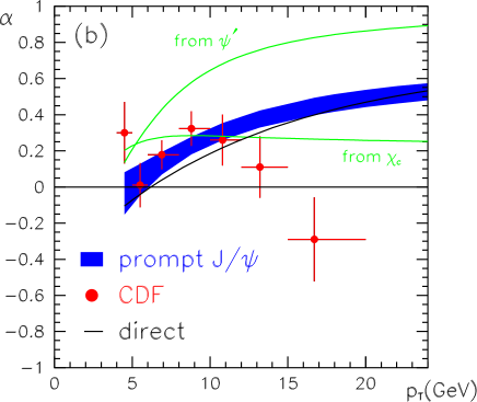
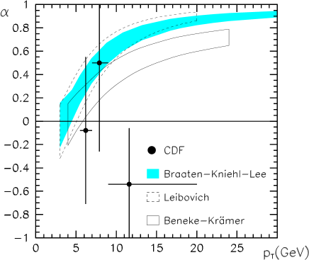
Figure 14: Left-hand side: $J/\psi$ polarization at the Tevatron. The band is the total NRQCD-factorization prediction. The other curves give the contributions from feeddown from higher charmonium states. Right-hand side: $\psi^{\prime}$ polarization at the Tevatron. The bands give various NRQCD-factorization predictions. The data points are from the CDF measurement [48]. From Ref. [46].

The degree of polarization is $\alpha=(1-3\xi)/(1+\xi)$, where $\xi$ is the fraction of events with longitudinal polarization. $\alpha=1$ corresponds to 100% transverse polarization, and $\alpha=-1$ corresponds to 100% longitudinal polarization. The observed polarization is in relatively good agreement with the prediction, except in the highest $p_{T}$ bin, although the prediction of increasing polarization with increasing $p_{T}$ is not in evidence.

Because the polarization depends on a ratio of matrix elements, some of the theoretical uncertainties are reduced compared with those in the production cross section, and, so, the polarization is probably not strongly affected by multiple soft-gluon emission or $K$ factors. Contributions of higher order in $\alpha_{s}$ could conceivably change the rates for the various spin states by a factor of two. Therefore, it is important to carry out the NLO calculation, which involves significant computational difficulties. It is known that order-$v^{2}$ corrections to parton fragmentation into quarkonium can be quite large [49]. If spin-flip corrections to the NRQCD matrix elements, which are nominally suppressed by powers of $v$, are also large, perhaps because the velocity-scaling rules need to be modified, then spin-flip contributions could significantly dilute the $J/\psi$ polarization. Nevertheless, in the context of NRQCD, it is difficult to see how there could not be substantial charmonium polarization for $p_{T}>4m_{c}$.

Compared to the $J/\psi$-polarization prediction, the $\Upsilon$-polarization prediction has smaller $v$-expansion uncertainties. However, because of the higher $\Upsilon$ mass, it is necessary to go to higher $p_{T}$ to insure that fragmentation dominates and that there is substantial polarization. Unfortunately, the current Tevatron data run out of statistics in this high-$p_{T}$ region. CDF finds that $\alpha=-0.12\pm 0.22$ for $8<p_{T}<20\hbox{ GeV}$ [50], which is consistent with both the NRQCD-factorization prediction [51] and the zero-polarization prediction of the CEM. There are also discrepancies between the polarizations observed in fixed-target experiments and the NRQCD predictions.

Calculations of inclusive $J/\psi$ and $\Upsilon$ production in $\gamma\gamma$ collisions [52, 53] have been compared with LEP data [54, 55, 56]. Both the $J/\psi$ and $\Upsilon$ measurements favor the NRQCD predictions over those of the color-singlet model.

Belle [57] and BaBar [58] have also measured the $J/\psi$ total cross sections in $e^{+}e^{-}\rightarrow J/\psi X$. The results of the two experiments are incompatible with each other, but they both seem to favor NRQCD over the color-singlet model. A surprising new result from Belle [59] is that most of the produced $J/\psi$’s are accompanied by an additional $c\overline{c}$ pair: $\sigma(e^{+}e^{-}\rightarrow J/\psi\,c\overline{c})/\sigma(e^{+}e^{-}\rightarrow J/\psi\,X)=0.59^{+0.15}_{-0.13}\pm 0.12$. Perturbative QCD plus the color-singlet model predict that this ratio should be about $0.1$ [60]. There seems to be a major discrepancy between theory and experiment. However, the order-$\alpha_{s}^{2}$ calculation lacks color-octet contributions, including those that produce $J/\psi\,c\overline{c}$. Although these contributions are suppressed by $v^{4}\approx 0.1$, it is possible that the short-distance coefficients are large. In other results, the angular distributions favor NRQCD, but the polarization measurements show no evidence of the transverse polarization that would be expected in color-octet production. However, the center-of-mass momentum is rather small, and, hence, one would not expect the polarization to be large.

Quarkonium production has also been measured in inelastic photoproduction [61, 62] and deep-inelastic scattering (DIS) [63, 64] at HERA. The NRQCD calculation deviates from the data near large photon-momentum fractions, owing to the large LO color-octet contribution. The NLO color-singlet result agrees with the data over all momentum fractions, as well as with the data as a function of $p_{T}$. See Ref. [40] for a more complete review. In the case of deep-inelastic scattering, the $Q^{2}$ and $p_{T}$ dependences are in agreement with NRQCD, but the results are more ambiguous for the dependence on the longitudinal momentum fraction.

3.3.3 Quarkonium Production in Nuclear Matter

The existing factorization “theorems” for quarkonium production in hadronic collisions are for cold hadronic matter. These theorems predict that nuclear matter is “transparent” for $J/\psi$ production at large $p_{T}$. That is, at large $p_{T}$, all of the nuclear effects are contained in the nuclear parton distributions. The corrections to this transparency are of order $(m_{Q}v/p_{T})^{2}$ for unpolarized cross sections and of order $m_{Q}v/p_{T}$ for polarized cross sections.

The effects of transverse-momentum kicks from multiple elastic collisions between active partons and spectators in the nucleons are among those effects that are suppressed by $(m_{Q}v/p_{T})^{2}$. Nevertheless, these multiple-scattering effects can be important because the production cross section falls steeply with $p_{T}$ and because the number of scatterings grows linearly with the path length through nuclear matter. Such elastic interactions can be expressed in terms of eikonal interactions [65] or higher-twist matrix elements [66].

Inelastic scattering of quarkonium by nuclear matter is also an effect of higher order in $(m_{Q}v/p_{T})^{2}$. However, it can become dominant when the amount of nuclear matter that is traversed by the quarkonium is sufficiently large. Factorization breaks down when

$$L\mathrel{\raise 1.29167pt\hbox{$>$\kern-7.5pt\lower 4.30554pt\hbox{$\sim$}}}{{\rm min}(z_{Q},z_{\overline{Q}})P_{H}^{2}\over M_{A}k_{T}^{2}({\rm tot})}\,\,,$$ (5)

where $L$ is the length of the quarkonium path in the nucleus, $M_{A}$ is the mass of the nucleus, $z$ is the parton longitudinal momentum fraction, $P_{H}$ is the momentum of the quarkonium in the parton CM frame, and $k_{T}({\rm tot})$ is the accumulated transverse momentum “kick” from passage through the nuclear matter. This condition for the breakdown of factorization is similar to “target-length condition” in Drell-Yan production [67, 68]. Such a breakdown is observed in the Cronin effect at low $p_{T}$ and in Drell-Yan production at low $Q^{2}$, where the cross section is proportional to $A^{\alpha}$, and $\alpha<1$.

It is possible that multiple-scattering effects may be larger for color-octet production than for color-singlet production. In the case of color-octet production, the pre-quarkonium $Q\overline{Q}$ system carries a nonzero color charge and, therefore, has a larger amplitude to exchange soft gluons with spectator partons.

At present, there is no complete, rigorous theory to account for all of the effects of multiple scattering and we must resort to “QCD-inspired” models. A reasonable requirement for models is that they be constructed so that they are compatible with the factorization result in the large-$p_{T}$ limit. Many models treat interactions of the pre-quarkonium with the nucleus as on-shell (Glauber) scattering. This assumption should be examined carefully, as on-shell scattering is known, from the factorization proofs, not to be a valid approximation in leading order in $(m_{Q}v/p_{T})^{2}$.

3.3.4 NRQCD Predictions for the LHC

In this section, we shall use the formalism of NRQCD to give predictions for quarkonium production in the LHC energy range. We rewrite the cross section in Eq. (4) for the inclusive production of a charmonium state $H$ as follows:

$$\sigma(H)\;=\;\sum_{n}\sigma^{(Q\overline{Q})_{n}}\;\langle{\cal O}^{H}_{n}\rangle\,\,,$$ (6)

where $\sigma^{(Q\overline{Q})_{n}}=F_{n}(\Lambda)/m_{Q}^{d_{n}-4}$, $\langle{\cal O}_{n}^{H}\rangle=\langle 0|{\cal O}_{n}^{H}|0\rangle$, and $n$ runs over all the color and angular momentum states of the $Q\overline{Q}$ pair. The cross sections $\sigma^{(Q\overline{Q})_{n}}$ can be calculated in perturbative QCD. All dependence on the final state $H$ is contained in the nonperturbative NRQCD matrix elements $\langle{\cal O}^{H}_{n}\rangle$.

The most important matrix elements for $J/\psi=\psi(1S)$ and $\psi^{\prime}=\psi(2S)$ production can be reduced to the color-singlet parameter $\langle{\cal O}^{\psi(nS)}_{1}(^{3}S_{1})\rangle$ and the three color-octet parameters $\langle{\cal O}^{\psi(nS)}_{8}(^{3}S_{1})\rangle$, $\langle{\cal O}^{\psi(nS)}_{8}(^{1}S_{0})\rangle$, and $\langle{\cal O}^{\psi(nS)}_{8}(^{3}P_{0})\rangle$. Two of the three color-octet matrix elements only appear in the linear combination

$$M_{k}^{\psi(nS)}=(k/m_{c}^{2})\langle{\cal O}^{\psi(nS)}_{8}(^{3}P_{0})\rangle+\langle{\cal O}^{\psi(nS)}_{8}(^{1}S_{0})\rangle\,\,.$$ (7)

The value of $k$ is sensitive to the $p_{T}$ dependence of the fit. At the Tevatron, $k\approx 3$. Fits to fixed-target total cross sections give larger values, $k\approx\hbox{6--7}$ [69]. The most important matrix elements for $\chi_{cJ}$ production can be reduced to a color-singlet parameter $\langle{\cal O}^{\chi_{c0}}_{1}(^{3}P_{0})\rangle$ and a single color-octet parameter $\langle{\cal O}^{\chi_{c0}}_{8}(^{3}S_{1})\rangle$. These matrix elements are sufficient to calculate the prompt $J/\psi$ cross section to leading order in $\alpha_{s}$ and to order $v^{4}$ relative to the color-singlet contribution.

Table 11: Matrix elements for charmonium production. Note that here $\langle{\cal O}_{1}^{H}\rangle=\langle{\cal O}_{1}^{\psi(nS)}(^{3}S_{1})\rangle$ for $J/\psi$ and $\psi^{\prime}$, but $\langle{\cal O}_{1}^{H}\rangle=\langle{\cal O}_{1}^{\chi_{c0}}(^{3}P_{0})\rangle$ for $\chi_{c0}$. Uncertainties are statistical only. From Ref. [46].

$$\begin{array}[]{|c|cccc|}\hline\cr\hline\cr H&\langle{\cal{O}}_{1}^{H}\rangle&\langle{\cal{O}}_{8}^{H}(^{3}S_{1})\rangle&k&M_{k}^{H}\\ \hline\cr J/\psi&1.3\pm 0.1~{}{\rm GeV^{3}}&(4.4\pm 0.7)\times 10^{-3}~{}{\rm GeV}^{3}&3.4&(8.7\pm 0.9)\times 10^{-2}~{}{\rm GeV}^{3}\\[-2.84526pt] \psi^{\prime}&0.65\pm 0.06~{}{\rm GeV^{3}}&(4.2\pm 1.0)\times 10^{-3}~{}{\rm GeV}^{3}&3.5&(1.3\pm 0.5)\times 10^{-2}~{}{\rm GeV}^{3}\\[-2.84526pt] \chi_{c0}&(8.9\pm 1.3)\times 10^{-2}~{}{\rm GeV^{5}}&(2.3\pm 0.3)\times 10^{-3}~{}{\rm GeV}^{3}&&\\[2.84526pt] \hline\cr\hline\cr\end{array}$$

In $pp$ collisions, different partonic processes for $Q\overline{Q}$ production dominate in different $p_{T}$ ranges. If $p_{T}$ is of order $m_{Q}$, fusion processes dominate, and, so, the $Q\overline{Q}$ pair is produced in the hard-scattering process. These contributions can be written in the form

$$\sigma_{\rm Fu}(H)=\sum_{i,j}\int dx_{1}\,dx_{2}\,f_{i/A}(x_{1},\mu^{2})f_{j/B}(x_{2},\mu^{2})\hat{\sigma}_{ij}^{(Q\overline{Q})_{n}}\;\langle{\cal O}^{H}_{n}\rangle\,\,,$$ (8)

where $A$ and $B$ are the incoming hadrons or nuclei. In Eq. (8), we include the parton processes $ij\rightarrow Q\overline{Q}\,X$, where $ij=gg,q\overline{q},qg$ and $\overline{q}g$, and $q=u,d,s$. The relevant partonic cross sections $\hat{\sigma}_{ij}^{(Q\overline{Q})_{n}}$ are given in Refs. [70, 71].

For $p_{T}\gg m_{Q}$, the dominant partonic process is gluon fragmentation through the color-octet ${}^{3}S_{1}$ channel. This contribution can be expressed as

$$\sigma_{\rm Fr}(H)=\sum_{i,j}\int dx_{1}\,dx_{2}\,dzf_{i/A}(x_{1},\mu^{2})f_{j/B}(x_{2},\mu^{2})\hat{\sigma}_{ij}^{g}D_{g}^{(Q\overline{Q})_{8}({}^{3}S_{1})}(z,\mu_{\rm Fr}^{2})\;\langle{\cal O}^{H}_{n}\rangle\,\,,$$ (9)

where $D_{g}^{(Q\overline{Q})_{n}({}^{3}S_{1})}(z,\mu_{\rm Fr}^{2})$ is the fragmentation function for a gluon fragmenting into a $Q\overline{Q}$ pair, $P/z$ is the momentum of the fragmenting gluon, $P$ is the momentum of the $Q\overline{Q}$ pair, and $\mu_{\rm Fr}$ is the fragmentation scale. The fragmentation process scales as $d\hat{\sigma}/dp_{T}^{2}\sim 1/p_{T}^{4}$ [72, 73]. The fragmentation process is actually included in the fusion processes of Eq. (8). In the limit $p_{T}\gg m_{Q}$, the fusion processes that proceed through $g^{*}\rightarrow(Q\overline{Q})_{8}({}^{3}S_{1})$ are well-approximated by the expression (9). At large $p_{T}$, one can evolve the fragmentation function in the scale $\mu_{\rm Fr}$, thereby resumming large logarithms of $p_{T}^{2}/m_{Q}^{2}$. Such a procedure leads to a smaller short-distance factor [45] and a more accurate prediction at large $p_{T}$ than would be obtained by using the fusion cross section (8). However, in our calculations, we employ the fusion cross section (8), which leads to systematic over-estimation of the cross section at large $p_{T}$.

In order to predict the cross section for prompt $J/\psi$ production (including $\chi_{c}$ and $\psi^{\prime}$ feeddown) at the LHC, we need the values of the NRQCD matrix elements. There have been several previous extractions of the color-octet matrix elements [45, 46, 70, 71, 74, 75, 76] from the CDF $J/\psi$, $\chi_{c}$ and $\psi^{\prime}$ $p_{T}$ distributions [39, 77]. We use the matrix elements given in Ref. [46], which are shown in Table 11. Our calculations are based on the MRST LO parton distributions [78].

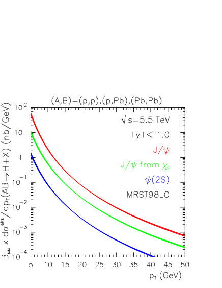
Figure 15: Differential cross sections per nucleon multiplied by leptonic branching fractions for prompt $J/\psi$ (upper curves), $J/\psi$ from $\chi_{c}$ (middle curves), and prompt $\psi(2S)$ (lower curves) in $pp$, $p$Pb, and Pb+Pb collisions at $\sqrt{s}=5.5$ TeV. The EKS98 parameterization [16, 17] is employed for $p$Pb and Pb+Pb collisions.

In calculating the cross section per nucleon for prompt $J/\psi$ production in $pA$ or $AA$ collisions, we take $f_{i/A}=f_{i/p}R^{A}_{i}$. We employ the EKS98 parameterization [16, 17] for the nuclear shadowing ratio $R^{A}_{i}$. We evolve $\alpha_{s}$ at one-loop accuracy, and we set $\mu=(4m_{c}^{2}+p_{T}^{2})^{1/2}$ and $m_{c}=1.5$ GeV.

There are several sources of uncertainty in our predictions for the cross sections. There are large uncertainties in the NRQCD matrix elements themselves. The errors shown in Table 11 are statistical only. There are additional large uncertainties in the matrix elements that arise from truncations of the series in $\alpha_{s}$ and $v$ in the theoretical expressions that are used to extract the matrix elements. The matrix elements $\langle{\cal O}_{8}(^{1}S_{0})\rangle$ and $\langle{\cal O}_{8}(^{3}P_{0})\rangle$ are fixed by the data only in the linear combination $M_{k}^{H}$. In the present calculation, we take $\langle{\cal O}_{8}(^{1}S_{0})\rangle=xM_{k}^{H}$ and $\langle{\cal O}_{8}(^{3}P_{0})\rangle/m_{c}^{2}=(1-x)M_{k}^{H}/k$, use the values of $k$ given in Table 11, and choose $x=1/2$. Variation of $x$ between $0$ and $1$ affects the cross sections at low $p_{T}$ by amounts on the order of 5%. There are additional uncertainties in the predicted cross sections that arise from the choices of the parton distributions, the charm-quark mass $m_{c}$, and the scale $\mu$. Because they affect the matrix-element fits, these uncertainties are highly correlated with those of the matrix elements. We have not tried to estimate their effects on the predicted cross sections.

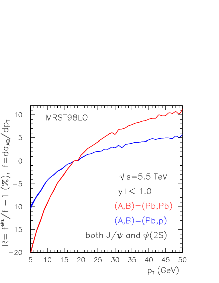
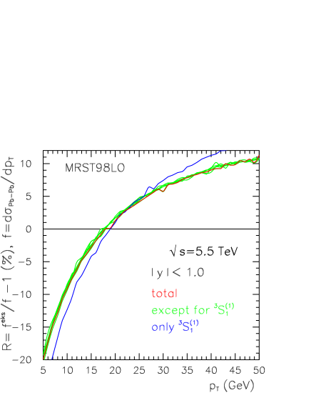
Figure 16: The $p_{T}$ dependence of $R_{AB}$ [Eq. (10)]. (a) We compare the results for $p$Pb and Pb+Pb collisions. (The $p_{T}$ dependence is stronger in the Pb+Pb result.) (b) We show the dependence of $R_{AB}$ on the various production channels in Pb+Pb collisions at $\sqrt{s}=5.5$ TeV.

In Fig. 15, we show the $p_{T}$ distributions per nucleon multiplied by the dilepton branching fractions for prompt $J/\psi$ (upper curves), $J/\psi$ from $\chi_{c}$ decays (middle curves), and prompt $\psi^{\prime}$ (lower curves) at $\sqrt{s}=5.5$ TeV. For $p$Pb and Pb+Pb collisions, we use the EKS98 parameterization [16, 17] to account for the effect of nuclear shadowing. The $pp$, $p$Pb, and Pb+Pb results essentially lie on top of each other in Fig. 15, owing to the many decades covered in the plot.

In order to display small differences between the distributions, we define the function $R_{AB}$:

$$R_{AB}(p_{T})=\frac{d\sigma_{AB}/dp_{T}-d\sigma_{pp}/dp_{T}}{d\sigma_{pp}/dp_{T}}\,\,.$$ (10)

In Fig. 16, we present $R_{AB}$ as a function of $p_{T}$. As is shown in Fig. 16(a), nuclear shadowing increases the cross section at large $p_{T}$ and decreases it at small $p_{T}$. The deviation of the Pb+Pb cross section from the $pp$ cross section is twice as large as that seen in the case of $p$Pb collisions. In order to investigate the dependence of the shadowing effect on the short-distance cross sections that arise in hadroproduction of $S$-wave charmonium states in Pb+Pb collisions, we plot $R_{AB}$ for all channels separately. [See Fig. 16(b).] Even though the $p_{T}$ dependence the contribution to the cross section of the color-octet ${}^{3}S_{1}$ channel is quite different from those of the color-octet ${}^{1}S_{0}$ and ${}^{3}P_{J}$ channels, all three channels show the same nuclear effect. The only channel that shows a slightly different behavior is the color-singlet channel, which gives a negligible contribution to the cross section. While the differential cross sections in Fig. 15 are strongly dependent on the nonperturbative NRQCD matrix elements, $R_{AB}$ is almost independent of the matrix elements, making it a good observable for studying nuclear shadowing at the LHC.

The $\Upsilon$ rates are somewhat more difficult to calculate because of the many feeddown contributions. The matrix elements are also not particularly well known. Since it is unlikely that all the different contributions can be disentangled, we follow the approach of Ref. [41] and compute the inclusive $\Upsilon(nS)$ production cross section

$$d\sigma(\Upsilon(nS))_{\rm inc} = d\sigma^{(b\overline{b})_{1}(^{3}S_{1})}\langle{\cal O}_{1}^{\Upsilon(nS)}(^{3}S_{1})\rangle_{\rm inc}+\sum_{J}d\sigma^{(b\overline{b})_{1}(^{3}P_{J})}\langle{\cal O}_{1}^{\Upsilon(nS)}(^{3}P_{J})\rangle_{\rm inc}$$ (11)

$$+\mbox{}d\sigma^{(b\overline{b})_{8}(^{3}S_{1})}\langle{\cal O}_{8}^{\Upsilon(nS)}(^{3}S_{1})\rangle_{\rm inc}+d\sigma^{(b\overline{b})_{8}(^{1}S_{0})}\langle{\cal O}_{8}^{\Upsilon(nS)}(^{1}S_{0})\rangle_{\rm inc}$$

$$+\left(\sum_{J}(2J+1)d\sigma^{(b\overline{b})_{8}(^{3}P_{J})}\right)\langle{\cal O}_{8}^{\Upsilon(nS)}(^{3}P_{0})\rangle_{\rm inc}\,\,,$$

where the last term makes use of heavy-quark spin symmetry to relate all of the octet ${}^{3}P_{J}$ matrix elements to the octet ${}^{3}P_{0}$ matrix element. The “inclusive” matrix elements are defined by

$$\langle{\cal O}_{i}^{\Upsilon(nS)}(n)\rangle_{\rm inc}=\sum_{H}B_{H\rightarrow\Upsilon(nS)}\langle{\cal O}_{i}^{H}(n)\rangle\,\,,$$ (12)

where $i=1$ or 8 for singlet or octet, respectively.

Table 12: Inclusive color-singlet matrix elements for bottomonium production. The errors on the ${}^{3}S_{1}$ matrix elements come from estimates of the $\Upsilon(nS)$ decay rate to lepton pairs. The errors on the ${}^{3}P_{J}$ states come from an average over potential-model estimates. The inclusive matrix elements are a linear combination of branching ratios, as in Eq. (12). The $S$-state matrix elements are in units of GeV³ while the $P_{J}$-state matrix elements are in units of GeV⁵. From Ref. [41].

$$\begin{array}[]{|c|cccc|}\hline\cr\hline\cr H&\langle{\cal{O}}_{1}^{H}(^{3}S_{1})\rangle_{\rm inc}&\langle{\cal{O}}_{1}^{H}(^{3}P_{0})\rangle_{\rm inc}&\frac{1}{3}\langle{\cal{O}}_{1}^{H}(^{3}P_{1})\rangle_{\rm inc}&\frac{1}{5}\langle{\cal{O}}_{1}^{H}(^{3}P_{2})\rangle_{\rm inc}\\ \hline\cr\Upsilon(3S)&4.3\pm 0.9&0&0&0\\[-2.84526pt] \Upsilon(2S)&5.0\pm 0.7&0.12\pm 0.06&0.55\pm 0.15&0.42\pm 0.10\\[-2.84526pt] \Upsilon(1S)&12.8\pm 1.6&<0.2&1.23\pm 0.25&0.84\pm 0.15\\[-2.84526pt] \hline\cr\hline\cr\end{array}$$

The sum over $H$ includes the $\Upsilon(nS)$ as well as all higher states that can decay to $\Upsilon(nS)$. The branching ratio for $H\rightarrow H^{\prime}$ decays is $B_{H\rightarrow H^{\prime}}$ with $B_{H\rightarrow H}\equiv 1$. Only $\chi_{b}(1P)$ and $\chi_{b}(2P)$ decays are included; the possibility of feeddown from the as-yet unobserved $\chi_{b}(3P)$ states is neglected. In the linear combination $M_{k}^{\Upsilon(nS)}$, the color-octet matrix element from the ${}^{3}P_{0}$ state is neglected, and, so, $M_{k}^{\Upsilon(nS)}=\langle{\cal O}_{8}^{\Upsilon(nS)}(^{1}S_{0})\rangle_{\rm inc}$. We use $m_{b}=4.77$ GeV and the MRST LO parton distributions. The values of the inclusive color-singlet matrix elements are given in Table 12, and the values of the inclusive color-octet matrix elements, from Ref. [41], are given in Table 13.

Table 13: Inclusive color-octet matrix elements for bottomonium production. The matrix elements were fit using the MRSTLO parton distributions. The first set of error bars is from $\chi^{2}$ fits to the $\Upsilon$ $p_{T}$ distributions in the region $p_{T}>8$ GeV. The second set is associated with the variation of the scales and corresponds to multiplying $\mu=\sqrt{m_{b}^{2}+p_{T}^{2}}$ by 2 (upper error) and 0.5 (lower error). The matrix elements are in units of $10^{-2}$ GeV³. From Ref. [41].

$$\begin{array}[]{|c|ccc|}\hline\cr\hline\cr H&\langle{\cal{O}}_{8}^{H}(^{3}S_{1})\rangle_{\rm inc}&\langle{\cal{O}}_{8}^{H}(^{1}S_{0})\rangle_{\rm inc}&\frac{5}{m_{b}^{2}}\langle{\cal{O}}_{1}^{H}(^{3}P_{0})\rangle_{\rm inc}\\ \hline\cr\Upsilon(3S)&3.7\pm 1.7^{+1.7}_{-1.3}&7.5\pm 4.9^{+3.4}_{-2.5}&0\\[-2.84526pt] \Upsilon(2S)&19.6\pm 6.3^{+8.9}_{-6.5}&-8.7\pm 11.1^{-2.4}_{+1.8}&0\\[-2.84526pt] \Upsilon(1S)&11.7\pm 3.0^{+5.7}_{-4.2}&18.1\pm 7.2^{+11.4}_{-8.1}&0\\[-2.84526pt] \hline\cr\hline\cr\end{array}$$

In Fig. 17, we show the $p_{T}$ distributions per nucleon multiplied by the dilepton branching fractions for the 3 $\Upsilon$ $S$ states at $\sqrt{s}=5.5$ TeV. The feeddown contributions are included as in Eq. (11). For $p$Pb and Pb+Pb collisions, we use the EKS98 parameterization [16, 17] in order to account for the effects of nuclear shadowing. The $pp$, $p$Pb, and Pb+Pb results lie essentially on top of each other in Fig. 17.

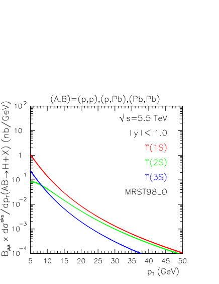
Figure 17: Differential cross sections per nucleon multiplied by leptonic branching fractions for inclusive $\Upsilon(1S)$ (upper curves), $\Upsilon(2S)$ (middle curves), and prompt $\Upsilon(3S)$ (lower curves) in $pp$, $p$Pb, and Pb+Pb collisions at $\sqrt{s}=5.5$ TeV. The EKS98 parameterization [16, 17] is employed for $p$Pb and Pb+Pb collisions.

The unusual relative behavior of the $\Upsilon(2S)$ and $\Upsilon(3S)$ states at both low and high $p_{T}$ is due to the fact that the bottomonium matrix elements are not very well determined. For $p_{T}<10$ GeV, the $\Upsilon(2S)$ cross section drops below the $\Upsilon(3S)$ cross section because the $\Upsilon(2S)$ has a large negative color-octet matrix element. (See Table 13.) The short-distance coefficients multiplying $M_{k}^{\Upsilon(nS)}$ are significant at low $p_{T}$. Thus, there is a large cancellation between the octet ${}^{3}S_{1}$ matrix element and $M_{k}^{\Upsilon(nS)}$, which reduces the $\Upsilon(2S)$ cross section in this region, causing it to drop below the $\Upsilon(3S)$ cross section at low $p_{T}$. At the high-$p_{T}$ end of the spectrum, the large value of the ${}^{3}S_{1}$ $\Upsilon(2S)$ color-octet matrix element (Table 13) causes the $\Upsilon(2S)$ cross section to approach that of the $\Upsilon(1S)$. In this region, the color-octet ${}^{3}S_{1}$ contribution dominates the other channels. Its large matrix element gives the $\Upsilon(2S)$ an unreasonably large cross section relative to that of the $\Upsilon(1S)$. The $\Upsilon(2S)$ rate at $p_{T}\approx 15$ GeV is more reasonable because the large and positive ${}^{3}S_{1}$ contribution, and the large and negative $M_{k}^{\Upsilon(2S)}$ contribution nearly cancel each other.

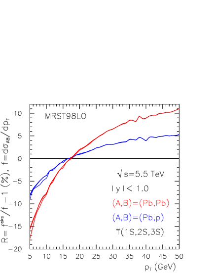
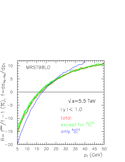
Figure 18: The $p_{T}$ dependence of $R_{AB}$ [Eq. (10)] for $\Upsilon$ production. (a) We compare the results for $p$Pb and Pb+Pb collisions. (The $p_{T}$ dependence is stronger in the Pb+Pb result.) (b) We show the dependence of $R_{AB}$ on the various production channels in Pb+Pb collisions at $\sqrt{s}=5.5$ TeV.

Better determinations of the $\Upsilon$ matrix elements are required in order to make more accurate predictions of the NRQCD $\Upsilon$-production rates at the LHC. As is shown in the $\Upsilon$-polarization analysis in Ref. [51], some theoretical predictions have quite large uncertainties even at Tevatron energies, owing to our poor knowledge of the matrix elements. However, as is shown in Fig. 18, the ratio $R_{AB}$ is still a good measure of the effect of shadowing on $\Upsilon$ production. The ratio is independent of the $\Upsilon$ state and is quite similar to the $J/\psi$ ratio in Fig. 16. The shadowing effect in Pb+Pb interactions may be somewhat less for the $\Upsilon$ at $p_{T}\approx 5$ GeV than for the $J/\psi$, but the difference is small. Note also, from Fig. 18(b), that $R_{AB}$ is essentially independent of the matrix elements and is, therefore, largely unaffected by their uncertainties.

3.4 Comparison of CEM and NRQCD Results 

Here we briefly compare the $p_{T}$ distributions of inclusive $J/\psi$ and $\Upsilon$ production in Pb+Pb collisions at 5.5 TeV calculated in the CEM and NRQCD approaches. Neither calculation includes any intrinsic transverse momentum effects which could alter the slopes of the $p_{T}$ distributions.

The $J/\psi$ distributions are compared on the left-hand side of Fig. 19. The NRQCD result from Fig. 15 is given in the solid curve. The branching ratio to lepton pairs has been removed and the cross section converted to $\mu$b. The CEM results from Fig. 12 are shown in the histograms. In this case, the direct $J/\psi$ cross section has been converted to the inclusive cross section. Considering the difference in mass, scale and parton densities in the two approaches, $m_{c}=1.5$ GeV and $\mu=\sqrt{4m_{c}^{2}+p_{T}^{2}}$ with MRST98LO for NRQCD and the parameters in Table 5 for the CEM, the agreement is rather good over the $p_{T}$ range shown. However, the $p_{T}$ slopes appear to be somewhat different. Note also that the NRQCD calculations are made in the rapidity interval $|y|<1$ while the CEM results are integrated over all rapidity, affecting the relative normalization. We can expect a comparable level of agreement for the other charmonium states which have a $p_{T}$ dependence similar to that of the inclusive $J/\psi$ in Fig. 15.

Figure 19: The $p_{T}$ dependence of the NRQCD and CEM results for inclusive $J/\psi$ (left) and $\Upsilon$ (right) production in 5.5 TeV Pb+Pb collisions is compared. The curves are the NRQCD predictions while the histograms are the CEM predictions. On the left-hand side, the $J/\psi$ CEM predictions are $\psi 1$ (solid), $\psi 2$ (dashed), $\psi 3$ (dot-dashed) and $\psi 4$ (dotted). On the right-hand side the CEM $\Upsilon$ calculations are $\Upsilon 1$ (solid), $\Upsilon 2$ (dashed), $\Upsilon 3$ (dot-dashed) and $\Upsilon 4$ (dotted).

The inclusive $\Upsilon(1S)$ distributions are compared on the right-hand side of Fig. 19. Here also we have converted the NRQCD result to $\mu$b and divided out the branching ratio to lepton pairs. We again see a relatively good agreement of the calculations in the two approaches, despite some differences in the masses, scales and parton densities used, as in the case of the $J/\psi$. The rapidity $|y|<1$ cut on the NRQCD result is a smaller relative factor for $\Upsilon$ production due to the narrower $\Upsilon$ rapidity distribution, see Fig. 11. We note that the agreement of the two approaches for the $\Upsilon(2S)$ and $\Upsilon(3S)$ states would not be as good, primarily due to the poorly determined matrix elements for these states, as previously discussed.

3.5 The Comover Enhancement Scenario (CES) 

3.5.1 The Quarkonium Thermometer

The production of heavy $Q\overline{Q}$ quarkonia may offer valuable insights into QCD dynamics, complementary to those given by open heavy flavor production. In both cases, the creation of the heavy quark pair requires an initial parton collision of hardness ${\cal O}(m_{Q})$. Most of the time the heavy quarks hadronize independently of each other and are incorporated into separate hadrons. The QCD factorization theorem exploits the conservation of probability in the hadronization process to express the total heavy quark production cross section in terms of target and projectile parton distributions and a perturbative subprocess cross section such as $\sigma(gg\rightarrow Q\overline{Q})$.

The quarkonium cross section is a small fraction of the open flavor one and is thus not constrained by the standard QCD factorization theorems. Nevertheless, it is plausible that the initial $Q\overline{Q}$ production is governed by the usual parton distributions and hard subprocess cross sections with the invariant mass of the $Q\overline{Q}$ pair constrained to be close to threshold. Before the quarkonium emerges in the final state there can, however, be further interactions which, due to the relatively low binding energy, can either “make or break” the bound state. Quarkonium studies can thus give new information about the environment of hard production, from the creation of the heavy quark pair until its “freeze-out”. The quantum numbers of the quarkonium state furthermore impose restrictions on its interactions. Thus states with negative charge conjugation, $\psi(nS)$, or total spin $J=1$, $\chi_{c1}$, require the $Q\overline{Q}$ pair to interact at least once after its creation via $gg\rightarrow Q\overline{Q}$.

Despite an impressive amount of data on the production of several quarkonium states with a variety of beams and targets we still have a poor understanding of the underlying QCD dynamics. Thus quarkonia cannot yet live up to their potential as ‘thermometers’ of $AB$ collisions, where $A,B=\gamma^{(*)}$, hadron or nucleus. Rather, it appears that we need simultaneous studies and comparisons of several processes to gain insight into the production dynamics.

We will now summarize the successes and failures of the Color Singlet Model [79, 80], which we consider as a guideline for understanding the nature of the quarkonium production dynamics.

3.5.2 Successes and Failures of the Color Singlet Model

In the Color Singlet Model (CSM), the $Q\overline{Q}$ pair is directly prepared with the proper quantum numbers in the initial hard subprocess and further interactions are assumed to be absent. The quarkonium production amplitude is then given by the overlap of the non-relativistic wave function with that of the $Q\overline{Q}$ pair.

This model at NLO correctly predicts the normalization and momentum dependence of the $J/\psi$ photoproduction rate [40, 81]. While the absolute normalization of the CSM prediction is uncertain by a factor of $2-3$ there appears to be no need for any additional production mechanism for longitudinal momentum fractions $0.3\leq x_{F}\leq 0.9$ and $1\leq p_{T}^{2}\leq 60$ GeV². The comparison with leptoproduction data [82] is less conclusive since only LO CSM calculations exist.

The CSM underestimates the directly produced $J/\psi$ and $\psi^{\prime}$ hadroproduction rates by more than an order of magnitude. This is true both at low $p_{\perp}\mathrel{\raise 1.29167pt\hbox{$<$\kern-7.5pt\lower 4.30554pt\hbox{$\sim$}}}m_{c}$ (fixed target) [83] and at high $p_{\perp}\gg m_{c}$ (collider) [40]. Similar discrepancies for the $\Upsilon$ states [28, 84, 85] indicate that the anomalous enhancement does not decrease quickly with increasing quark mass.

The inelastic cross section ratio $\sigma(\psi^{\prime})/\sigma_{\rm dir}(J/\psi)$ is similar in photoproduction [86] and hadroproduction [87, 88] and consistent with the value $\simeq 0.24$ expected in the CSM [89]. The ratio does not depend on $x_{F}$ in the projectile fragmentation region and is independent of the nuclear target size in $hA$ collisions. The CSM thus underestimates the $J/\psi$ and $\psi^{\prime}$ hadroproduction cross sections, as well as that of the $\chi_{c1}$ [89], by similar large factors. The quantum numbers of these charmonium states require final-state gluon emission in the CSM, $gg\rightarrow J/\psi g$. This emission is not required for the $\chi_{c2}$ where the CSM cross section $\sigma(gg\rightarrow\chi_{c2})$ is only a factor $\sim 2$ below the hadroproduction data [89].

In the CSM, $\chi_{c}$ photoproduction is suppressed by a power of $\alpha_{s}$ compared to the $J/\psi$ and $\psi^{\prime}$ production rates. One indeed observes a smaller value of the $\sigma(\chi_{c2})/\sigma(J/\psi)$ ratio in photoproduction [90] than in hadroproduction [91, 92].

3.5.3 Description of the CES and its generic timescales

The analysis of agreements and discrepancies between the CSM and quarkonium data led to the comover enhancement scenario of quarkonium production [93, 94]. Hadroproduced $Q\overline{Q}$ pairs are created within a comoving color field and form $J/\psi$, $\psi^{\prime}$ and $\chi_{c1}$ through gluon absorption rather than emission, enhancing the cross section relative to the CSM since the pair gains rather than loses energy and momentum. The $\chi_{c2}$ cross section is not as strongly influenced since no gluon needs to be absorbed or emitted. Most importantly, such a mechanism is consistent with the success of the CSM in photoproduction since no color fields are expected in the photon fragmentation region, $x_{F}\mathrel{\raise 1.29167pt\hbox{$>$\kern-7.5pt\lower 4.30554pt\hbox{$\sim$}}}0.3$.

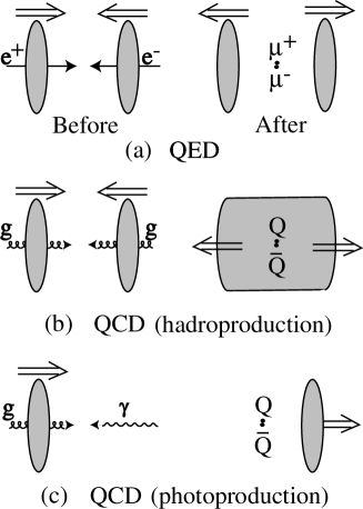
Figure 20: Schematic scenarios of gauge field interactions are compared: (a) $e^{+}e^{-}\rightarrow\mu^{+}\mu^{-}$ in QED; (b) hadroproduction of a $Q\overline{Q}$ pair, e.g. $gg\rightarrow Q\overline{Q}$; and (c) photoproduction of a $Q\overline{Q}$ pair, $\gamma g\rightarrow Q\overline{Q}$. The creation of a comoving color field is specific to hadroproduction, (b).

The origin of a comoving color field in hadroproduction is illustrated in Fig. 20. Light charged particles carry gauge fields which are radiated in high energy annihilations into a heavy particle pair. In $e^{+}e^{-}\rightarrow\mu^{+}\mu^{-}$ annihilations, the photon fields pass through each other and materialize as forward bremsstrahlung, Fig. 20(a). In $gg\rightarrow Q\overline{Q}$, on the other hand, the self-interaction of the color field can also result in the creation of a gluon field at intermediate rapidities, Fig. 20(b). Hadroproduced $Q\overline{Q}$ pairs thus find themselves surrounded by a color field. We postulate that interactions between the $Q\overline{Q}$ pair and this comoving field are important in quarkonium hadroproduction. In direct photoproduction, the incoming photon does not carry any color field and the $Q\overline{Q}$ pair is left in a field-free environment after the collision, Fig. 20(c). The proposed rescattering thus does not affect (non-resolved) photoproduction.

The importance of rescattering effects in hadroproduction as compared to photoproduction is also suggested by data on open charm production. Hadroproduced $D\overline{D}$ pairs are almost uncorrelated in azimuthal angle [95], at odds with standard QCD descriptions. Photoproduced pairs on the other hand, emerge nearly back-to-back [96], following the charm quarks of the underlying $\gamma g\rightarrow c\overline{c}$ process.

Since the hardness of the gluons radiated in the creation process increases with quark mass, the rescattering effect persists for bottomonium. Due to the short timescale of the radiation the heavy quark pair remains in a compact configuration during rescattering and overlaps with the quarkonium wave function at the origin. The successful CSM result for $\sigma(\psi^{\prime})/\sigma_{\rm dir}(J/\psi)$ [89] is thus preserved.

The $Q\overline{Q}$ pair may also interact with the more distant projectile spectators after it has expanded and formed quarkonium. Such spectator interactions are more frequent for nuclear projectiles and can cause the breakup (absorption) of the bound state. This conventional mechanism of quarkonium suppression in nuclei is thus fully compatible with, but distinct from, interactions with the comoving color field.

We have investigated the consequences of the CES using pQCD to calculate the interaction between the $Q\overline{Q}$ and the comoving field. While we find consistency with data, quantitative predictions depend on the structure of the comoving field. Hence tests of the CES must rely on its generic features, especially the proper timescales over which the $Q\overline{Q}$ proceeds from production through hadronization.

The CES distinguishes three proper timescales in quarkonium production:

• $\tau_{Q}\sim 1/m_{Q}$, the $Q\overline{Q}$ pair production time;

• $\tau_{AP}$, the DGLAP scale over which the comoving field is created and interacts with the $Q\overline{Q}$ pair;

• $\tau_{\Lambda}\sim 1/\Lambda_{\rm QCD}$, while rescattering with comoving spectators may occur.

In the following we will consider quarkonium production at $p_{\perp}\mathrel{\raise 1.29167pt\hbox{$<$\kern-7.5pt\lower 4.30554pt\hbox{$\sim$}}}m_{Q}$. In quarkonium production at $p_{T}\gg m_{Q}$, a large $p_{T}$ parton is first created on a timescale $1/p_{T}$, typically through $gg\rightarrow gg^{*}$. The virtual gluon then fragments, $g^{*}\rightarrow Q\overline{Q}$, in proper time $\tau_{Q}$. Thus high $p_{T}$ quarkonium production is also describable with the CES [97].

Timescale $\tau_{Q}\sim 1/m_{Q}$: creation of the $Q\overline{Q}$ pair —

The $Q\overline{Q}$ pair is created in a standard parton subprocess, typically $gg\rightarrow Q\overline{Q}$, at a time scale $\tau_{Q}\sim 1/m_{Q}$. This first stage is common to other theoretical approaches such as the CEM [98, 99, 100] and NRQCD [34, 69]. The momentum distribution of the $Q\overline{Q}$ is determined by the product of projectile $(A)$ and target $(B)$ parton distributions, such as $g_{A}(x_{1})g_{B}(x_{2})$ where $A$, $B$ may be a hadron, nucleus or resolved real or virtual photon. (In the case of direct photoproduction or DIS, when the projectile is a photon or lepton, the process depends on the single distribution $g_{B}(x_{2})$.) Such production is consistent with the quarkonium data.

According to pQCD, the $Q\overline{Q}$ is dominantly produced close to threshold in a color octet, $S=L=0$ configuration. Such a state can obtain the quarkonium quantum numbers through a further interaction which flips a heavy quark spin and turns the pair into a color singlet. The amplitude for processes of this type are suppressed by the factor $k/m_{Q}$ where $k$ is the momentum scale of the interaction. The various theoretical approaches differ in the scale assumed for $k$.

CSM: Here $k={\cal O}(m_{Q})$. Thus $J/\psi$ production proceeds via the emission of a hard gluon in the primary process, $gg\rightarrow Q\overline{Q}+g$. The $\chi_{c2}$ is produced without gluon emission, $gg\rightarrow\chi_{c2}$, through a subdominant $S=L=1$ color singlet production amplitude.

NRQCD: The $Q\overline{Q}$ quantum numbers are changed via gluon emission at the bound state momentum scale $k={\cal O}(\alpha_{s}m_{Q})$. This corresponds to an expansion in powers of the bound state velocity $v=k/m_{Q}$, introducing nonperturbative matrix elements that are fit to data.

CEM: Here $k={\cal O}(\Lambda_{\rm QCD})$. Soft interactions are postulated to change the $Q\overline{Q}$ quantum numbers with probabilities that are specific for each quarkonium state but independent of kinematics, projectile and target.

CES: The quantum numbers of the $Q\overline{Q}$ are changed in perturbative interactions with a comoving field at scale $k={\cal O}(1/\tau_{AP})$, as described below.

Timescale $\tau_{AP}$: interactions with the comoving field —

The scale $\tau_{AP}$ refers to the time in which collinear bremsstrahlung, the source of QCD scaling violations, is emitted in the heavy quark creation process [93]. Thus $1/\tau_{AP}$ characterizes the effective hardness of logarithmic integrals of the type $\int_{\mu_{F}}^{m_{Q}}dk/k$ where $\mu_{F}\ll m_{Q}$ is the factorization scale. We stress that $1/\tau_{AP}$ is an intermediate but still perturbative scale, $\tau_{Q}\ll\tau_{AP}\ll\tau_{\Lambda}$, which grows with $m_{Q}$.

The fact that the $Q\overline{Q}$ pair acquires the quarkonium quantum numbers over the perturbative timescale $\tau_{AP}$ is a feature of the CES and distinguishes it from other approaches. At this time, the pair is still compact and couples to quarkonia via the bound state wavefunction at the origin or its derivative(s). Thus no new parameters are introduced in this transition. However, the interactions of the $Q\overline{Q}$ pair depend on the properties of the comoving color field such as its intensity and polarization. Quantitative predictions in the CES are only possible when the dependence on the comoving field is weak.

Ratios of radially excited quarkonia, such as $\sigma(\psi^{\prime})/\sigma_{\rm dir}(J/\psi)$, are insensitive to the comoving field and are thus expected to be process-independent when absorption on spectators at later times can be ignored, see below. The fact that this ratio is observed to be roughly universal [87, 88] is one of the main motivations for the CES. Even the measured variations of the ratio in different reactions agree with expectations, see Ref. [101] for a discussion of its systematics in elastic and inelastic photoproduction, leptoproduction and hadroproduction at low and high $p_{T}$.

The ratio $\sigma(\chi_{c1})/\sigma(\chi_{c2})$ is measured to be $0.6\pm 0.3$ in pion-induced [102] and $0.31\pm 0.14$ in proton-induced [103] reactions. The CSM underestimates this ratio as well as that of $\sigma(J/\psi)/\sigma(\chi_{2})$ [89]. The rescattering contribution increases $\sigma(J/\psi)$ and $\sigma(\chi_{1})$, enhancing the above ratios.

Nuclear target dependence —

The quarkonium cross section can be influenced by rescattering effects in both the target and projectile fragmentation regions. For definiteness, we assume the charmonium is produced in the projectile fragmentation region, $x_{F}>0$.

The nuclear target dependence is usually parameterized as $\sigma(hA\rightarrow J/\psi+X)\propto A^{\alpha}$. Data show that $\alpha<1$ and obeys Feynman scaling: $\alpha$ depends on (and decreases with) $x_{F}$ rather than on the momentum fraction $x_{2}$ of the target parton [104, 105]. The comparison with lepton pair production in the Drell-Yan process shows that the $J/\psi$ nuclear suppression cannot be attributed to shadowing of parton distributions in the nucleus [88]. The $A$ dependence is thus difficult to explain in the CSM, NRQCD and CEM approaches.

In the Feynman scaling regime, we may assume that the $Q\overline{Q}$ pair energy is high enough to remain compact while traversing the target. The relative transverse momentum of the $Q$ and $\overline{Q}$ could increase as a result of rescattering in the target, thus suppressing the binding probability. However, this explanation is unlikely in view of the absence of nuclear suppression in photoproduction [106].

In the CES, the nuclear target suppression is ascribable to absorption of the comoving color field in the target nucleus. This field is emitted by a projectile parton with transverse size $\tau_{AP}$, larger than the size, $\sim 1/m_{Q}$, of the $Q\overline{Q}$ pair. Due to Lorentz time dilation, the field is emitted long before reaching the target and reinteracts with the $Q\overline{Q}$ long after passing the target. Absorption of the comoving field in the target implies suppression of $J/\psi$ production in the CES. At high energies, we have $x_{1}\simeq x_{F}$, which explains the Feynman scaling of this effect. Moreover, as $x_{F}$ increases, less energy is available to be radiated to the gluon field which therefore becomes softer, further increasing its absorption in the target and thus the nuclear suppression.

This explanation is consistent with the fact that the nuclear target suppression of the $J/\psi$ and the $\psi^{\prime}$ is found to be the same for $x_{F}\mathrel{\raise 1.29167pt\hbox{$>$\kern-7.5pt\lower 4.30554pt\hbox{$\sim$}}}0.2$ [105]. It also predicts that the suppression will be similar for $\chi_{c1}$ production. On the other hand, the nuclear target suppression should be reduced for $\chi_{c2}$ since a substantial fraction is directly produced without gluon absorption from the comoving field. A measurement of $\sigma(hA\rightarrow\chi_{c1},\chi_{c2}+X)$ in the projectile fragmentation region would thus constitute an important test of the CES.

In a Glauber picture of the nuclear suppression, a relatively large value for the absorption cross section is required, $\sigma_{\rm abs}\sim 5\ {\rm mb}$. We interpret this value as the joint cross section of the $Q\overline{Q}$ pair and the comoving field, thus of order $\tau_{AP}^{2}\gg 1/m_{Q}^{2}$. Since $1/\tau_{AP}$ scales with $m_{Q}$, we expect less nuclear absorption for the $\Upsilon$ states than for the $J/\psi$, as observed experimentally [107, 108].

Timescale $\tau_{\Lambda}\sim 1/\Lambda_{\rm QCD}$: interactions with comoving spectators —

By the time, $\tau_{\Lambda}\sim 1$ fm, that the $Q\overline{Q}$ pair encounters comoving projectile spectators, the pair has already expanded and is distributed according to the quarkonium wave function. The spectator rescattering effects are thus independent of the quarkonium formation process. Larger and more loosely bound charmonia are more easily broken up by secondary scattering. Hence the $\chi_{c}$ and $\psi^{\prime}$ cross sections should be depleted compared to that of the $J/\psi$. Likewise bottomonium is generally less affected by spectator interactions than charmonium.

Spectator interactions at large enough $x_{F}$ are likely to be unimportant for hadron projectiles judging from the approximate universality of the $\sigma(\psi^{\prime})/\sigma_{\rm dir}(J/\psi)$ ratio in photo- and hadroproduction. The lower ratio seen in nucleus-nucleus collisions [109], on the other hand, is most naturally explained by absorption on spectators. It would be important to confirm this by also measuring the ratio in $hA$ scattering in the nuclear fragmentation region.

3.5.4 Summary

Data on quarkonium production have proved challenging for QCD models. The richness of the observed phenomena indicates that quarkonium cross sections are indeed sensitive to the environment of the hard QCD scattering. We may, however, only be able to decipher its message through systematic experimental and theoretical studies of several species of quarkonia produced with a variety of beams and targets in a range of kinematic conditions.

The rates of quarkonium production at the LHC are large enough for high statistics studies of the production mechanism. Differences in $pp$ rates and $p_{T}$ distributions may help distinguish between the CEM, NRQCD and CES approaches.

Acknowledgments S. P. would like to thank Cristina Volpe for very stimulating discussions.

4 ABSORPTION AND ENERGY LOSS 

In this section, we first discuss $J/\psi$ absorption in matter by nucleons (sect. 4.1) and comoving secondaries (sect. 4.2). We then present a brief review of heavy quark energy loss (sect. 4.3).

The effective nucleon absorption cross sections in section 4.1 are obtained by extrapolating the values extracted from the fixed-target measurements to higher energies. The resulting charmonium suppression can be used as a baseline in the search for deconfinement.

In section 4.2, an evaluation of the couplings of the $J/\psi$ to $D^{(*)}D^{(*)}$ and $D^{(*)}D^{(*)}\pi$ are presented in the Constituent Quark Model. These couplings are a crucial ingredient in the calculation of cross sections for the processes $\pi J/\psi\rightarrow D^{(*)}\overline{D}^{(*)}$, an important background for the $J/\psi$ suppression signal in quark-gluon plasma. While final results relevant to the cross section for $J/\psi$ absorption by comovers are not yet available, the finished calculation should provide some of the most reliable results for these processes.

Energy loss has been much discussed in the context of jet quenching. While some calculations have addressed quarkonium, this aspect of energy loss is still too unsettled to be summarized. Therefore, only energy loss by heavy quarks in medium is evaluated in section 4.3.

4.1 Charmonium Suppression in Nuclear Collisions at the LHC: the baseline 

Suppression of the $J/\psi$ in nucleus-nucleus collisions was proposed as a signal of color deconfinement a long time ago [1]. Shortly after, such a suppression was observed in O+U and, subsequently, in S+U collisions [110, 111, 112]. It was promptly noted that at least part of the observed effect was already present in $pA$ collisions [113, 114]. A quantitative analysis of charmonium suppression in nuclear matter has been performed in Ref. [115]. Here we extend that analysis to RHIC and LHC energies, $\sqrt{s}=200$ GeV and 5.5 TeV respectively. In this extension, we assume that the increased energy does not change the nature of the nuclear absorption process. In principle, interference between successive scatterings could lead to modifications at higher energies. The forthcoming $p(d)A$ data from RHIC could clarify this point.

Apart from the independently-determined nuclear matter distributions, the only parameter entering the calculation is the effective absorption cross section of the quarkonium precursor in nuclear matter, determined from $pA$ data. The latest data indicate $\sigma_{\rm abs}\simeq 5$ mb [116, 117]. We assume that $\sigma_{\rm abs}$ increases with charmonium-nucleon center of mass energy as $s_{J/\psi N}^{\Delta}$, reflecting the growth of the small $x$ gluon density in nucleons. A massive $Q\overline{Q}$ state produced at zero rapidity will interact with nucleons at center of mass energy squared $s_{J/\psi N}\simeq 2m_{J/\psi}(\sqrt{s}/2)$ where $\sqrt{s}$ is the center of mass energy per nucleon pair of the heavy ion collision. Therefore, the effective absorption cross section will increase with $\sqrt{s}$ as

$$\sigma_{\rm abs}(\sqrt{s})=\sigma_{\rm abs}(\sqrt{s_{0}})\ \left({s\over s_{0}}\right)^{\Delta/2}\,\,.$$ (13)

Table 14: Effective charmonium–nucleon absorption cross sections at SPS, RHIC, and LHC energies. The middle row is the result for the central value of $\sigma_{\rm abs}(\sqrt{s_{0}})$ while the upper and lower rows show the errors on $\sigma_{\rm abs}$.

$\sigma_{\rm abs}$ (mb)
SPS	RHIC	LHC
4.5	6.1	9.3
5.0	6.8	10.3
5.5	7.5	11.3

We choose $\sqrt{s_{0}}\simeq 17.3$ GeV (the CERN SPS energy), $\sigma_{\rm abs}(\sqrt{s_{0}})=5\pm 0.5$ mb for charmonium, and $\Delta=0.125$. Note that since $\sigma_{\rm abs}$ is the absorption cross section of the precursor charmonium state, it is assumed to be the same for all charmonium resonances. With these parameters, the values of the absorption cross sections at RHIC and LHC are given in Table 14.

Figure 21: The energy dependence of $\sigma_{\rm abs}$.

The energy dependence of the absorption cross section is shown in Fig. 21.

The quarkonium survival probability in an $AB$ collision is given by, see Eq. (6) of Ref. [115],

$$S_{J/\psi}(b) = \int d^{2}s\int dz_{A}dz_{B}\rho_{A}(\vec{s},z_{A})\rho_{B}(\vec{b}-\vec{s},z_{B})$$

$$\times\exp\left\{-(A-1)\int_{z_{A}}^{\infty}dz_{A}^{\prime}\rho_{A}(\vec{s},z_{A}^{\prime})\sigma_{\rm abs}\right\}$$

$$\times\exp\left\{-(B-1)\int_{z_{B}}^{\infty}dz_{B}^{\prime}\rho_{B}(\vec{b}-\vec{s},z_{B}^{\prime})\sigma_{\rm abs}\right\}\,\,.$$

Table 15: $J/\psi$ survival probability in Pb+Pb collisions as a function of impact parameter for SPS, RHIC, and LHC energies. The central results are calculated with the value of $\sigma_{\rm abs}$ given in the middle row of Table 14. The errors represent the uncertainty in $\sigma_{\rm abs}$.

	$S_{J/\psi}$
$b$ (fm)	SPS	RHIC	LHC
$\langle b\rangle$	0.52 $\pm$ 0.03	0.42 $\pm$ 0.03	0.29 $\pm$ 0.03
0	0.47 $\pm$ 0.03	0.37 $\pm$ 0.04	0.25 $\pm$ 0.03
1	0.47 $\pm$ 0.03	0.37 $\pm$ 0.04	0.25 $\pm$ 0.03
2	0.47 $\pm$ 0.03	0.37 $\pm$ 0.04	0.25 $\pm$ 0.03
3	0.48 $\pm$ 0.03	0.38 $\pm$ 0.04	0.25 $\pm$ 0.03
4	0.48 $\pm$ 0.03	0.38 $\pm$ 0.04	0.25 $\pm$ 0.03
5	0.49 $\pm$ 0.03	0.39 $\pm$ 0.04	0.26 $\pm$ 0.03
6	0.50 $\pm$ 0.03	0.40 $\pm$ 0.04	0.27 $\pm$ 0.03
7	0.52 $\pm$ 0.03	0.42 $\pm$ 0.04	0.29 $\pm$ 0.03
8	0.54 $\pm$ 0.03	0.44 $\pm$ 0.03	0.31 $\pm$ 0.03
9	0.57 $\pm$ 0.03	0.47 $\pm$ 0.03	0.34 $\pm$ 0.03
10	0.60 $\pm$ 0.03	0.51 $\pm$ 0.03	0.38 $\pm$ 0.03
11	0.65 $\pm$ 0.03	0.57 $\pm$ 0.03	0.44 $\pm$ 0.03
12	0.71 $\pm$ 0.02	0.63 $\pm$ 0.03	0.51 $\pm$ 0.03

The resulting $J/\psi$ survival probability as a function of impact parameter in a Pb+Pb collision is given in Table 15 for SPS, RHIC and LHC energies.

Figure 22: The impact parameter dependence of $S_{J/\psi}$ in Pb+Pb and Ar+Ar collisions at the LHC. We assume $\sqrt{s}=5.5$ TeV for both systems. In both cases, the survival probabilities in the central curves are calculated with the median $\sigma_{\rm abs}$ extrapolated to LHC energies while the upper and lower curves give the uncertainty in $S_{J/\psi}$ due to the absorption cross section.

The LHC result is also shown in Fig. 22.

Table 16: The $J/\psi$ survival probability in Ar+Ar collisions at the LHC as a function of impact parameter. The central results are calculated with the value of $\sigma_{\rm abs}$ given in the middle row of Table 14. The errors represent the uncertainty in $\sigma_{\rm abs}$.

$b$ (fm)	$S_{J/\psi}$
$\langle b\rangle$	0.52 $\pm$ 0.03
0	0.45 $\pm$ 0.03
1	0.45 $\pm$ 0.03
2	0.46 $\pm$ 0.03
3	0.48 $\pm$ 0.03
4	0.51 $\pm$ 0.03
5	0.56 $\pm$ 0.03
6	0.62 $\pm$ 0.03
7	0.69 $\pm$ 0.02
8	0.77 $\pm$ 0.02

To illustrate the $A$ dependence, we have also calculated the survival probability in Ar+Ar collisions at the LHC. The results are shown in Table 16 and Fig. 22.

Figure 23: The centrality dependence of $S_{J/\psi}$ at the LHC in Pb+Pb and Ar+Ar collisions, both at $\sqrt{s}=5.5$ TeV. In both cases, the survival probabilities in the central curves are calculated with the median $\sigma_{\rm abs}$ extrapolated to LHC energies while the upper and lower curves give the uncertainty in $S_{J/\psi}$ due to the absorption cross section. $N_{\rm part}^{\rm max}=2A$ is the maximum number of participants.

Since the impact parameter of the collision cannot be measured directly, it is convenient to choose the number of participants, those nucleons that have participated in at least one inelastic collision, as a measure of centrality. At least in principle the number of participants, $N_{\rm part}$, can be inferred from the measurements of the number of spectator nucleons, $N_{\rm spect}$, going forward since $N_{\rm part}=A-N_{\rm spect}$. The survival probabilities in Pb+Pb and Ar+Ar collisions at the LHC are shown in Fig. 23 as a function of $N_{\rm part}/N_{\rm part}^{\rm max}$ where $N_{\rm part}^{\rm max}=2A$.

Figure 24: The dependence of $S_{J/\psi}$ on $N_{\rm part}$ for Pb+Pb collisions at SPS, RHIC and LHC energies.

Figure 24 the compares charmonium survival probabilities in Pb+Pb as a function of $N_{\rm part}$ at SPS, RHIC, and the LHC. The suppression due to nuclear absorption alone at the LHC is expected to be much stronger than at the SPS.

Finally we note that at the LHC, bottomonium production will be abundant enough for study of their suppression in hot matter to be feasible. Because of their smaller size and larger binding energy, the $\Upsilon$ states will provide valuable information complementary to the study of charmonium. The available E772 data on $\Upsilon$ production at $\sqrt{s}=39$ GeV [107, 118] imply an effective $b\overline{b}$ absorption cross section of $\sigma_{\rm abs}=2.5\pm 0.5$ mb. Assuming the energy dependence of this effective absorption cross section is the same as that of Eq. (13), we find $\sigma_{\rm abs}=4.6\pm 0.9$ mb at 5.5 TeV. The corresponding $\Upsilon$ survival probabilities are presented in Fig. 25.

Figure 25: The centrality dependence of the $\Upsilon$ survival probability at the LHC in Pb+Pb and Ar+Ar collisions. In both cases, the survival probabilities in the central curves are calculated with the median $\sigma_{\rm abs}$ extrapolated to LHC energies while the upper and lower curves give the uncertainty in $S_{J/\psi}$ due to the absorption cross section. $N_{\rm part}^{\rm max}=2A$ is the maximum number of participants.

4.2 A Note on the $J/\psi$ Strong Couplings 

In this section, we present a preliminary report on a study of $J/\psi$ absorption due to its interaction with the hot hadronic medium formed in relativistic heavy-ion collisions. We will give the full analysis elsewhere [119]. Here we concentrate on the strong couplings of the $J/\psi$ to low-mass charm mesons and pions. In the calculation of the relevant absorption cross sections, tree-level diagrams such as those depicted in Fig. 26 are encountered.

Figure 26: Feynman diagrams for $J/\psi$ absorption by the pion: (1) $J/\psi\pi\rightarrow D{\overline{D}}$, (2) $J/\psi\pi\rightarrow{\overline{D}}D^{*}$ and $J/\psi\pi\rightarrow{\overline{D}}^{*}D^{*}$.

Previous studies of these effects can be found in [120, 121, 122, 123]. Besides the $DD^{*}\pi$ couplings, for which both theoretical [124, 125, 126] and experimental [127] results are available, in Fig. 26 the $JD^{(*)}D^{(*)}$ and $JD^{(*)}D^{(*)}\pi$ couplings also appear (in this section, we shall often use $J$ to indicate the $J/\psi$). These couplings have been estimated by different methods, that are, in our opinion, unsatisfactory. For example, the use of SU(4) symmetry puts the charm quark and the light quarks on the same footing, at odds with the results obtained within the Heavy Quark Effective Theory (HQET), which treats the charm as infinitely massive, $m_{c}\gg\Lambda_{\rm QCD}$ (see Ref. [126]). Similarly, approaches based on Vector Meson Dominance (VMD) should be considered critically given the large extrapolation involved, $p^{2}=0\rightarrow m_{J/\psi}^{2}$. A different evaluation, based on QCD Sum Rules, presents the typical theoretical uncertainties of this method [128, 129]. Here, we take another approach, based on the Constituent Quark Model (CQM), a quark-meson model which explicitly takes into account the HQET symmetries. For more details on the CQM see Ref. [130, 131].

The CQM is particularly suitable for studies of exclusive heavy meson decays. Since its Lagrangian contains the Feynman rules for the heavy-light vertices formed by a heavy meson, transition amplitudes are computable via simple constituent quark loop diagrams where mesons enter as external legs. The model is relativistic and incorporates the chiral SU(2) symmetry of the light quark sector as well as the heavy quark symmetries. The calculation of the $DD^{*}\pi$ coupling in the CQM can be found in Ref. [130, 131]. Here we shall consider the calculation of the $JD^{(*)}D^{(*)}$ and $JD^{(*)}D^{(*)}\pi$ vertices within the CQM. This will be done by treating the $J/\psi$ with VMD, as depicted in Fig. 27, and computing the Feynman diagrams prescribed by the CQM.

Figure 27: The Vector Meson Dominance equation for the coupling of the $J/\psi$ with $D$ and $D^{*}$ in terms of the Isgur-Wise function $\xi$. The function $\xi$ on the left-hand side is computed by a diagram with a quark loop. The coupling of each $D^{(*)}$ meson to quarks is given by $\sqrt{Z_{H}m_{D}}$.

In the CQM, the evaluation of the loop diagram depicted on the left-hand side of Fig. 27 amounts to the calculation of the Isgur-Wise function [130, 131]. The result is

$$\xi(\omega)=Z_{H}\left[\frac{2}{1+\omega}I_{3}(\Delta_{H})+\left(m+\frac{2\Delta_{H}}{1+\omega}I_{5}(\Delta_{H},\Delta_{H},\omega)\right)\right]\ ,$$ (14)

where $m$ is the light constituent mass, $Z_{H}$ is a constant arising from the $D^{(*)}$ coupling to their constituent quarks so that the coupling constant is $\sqrt{Z_{H}m_{D}}$ [130, 131], and the $I_{i}$ integrals are listed in sect. 4.2.1. Here $\omega=v\cdot v^{\prime}$, the product of the two heavy quark velocities, $v$ and $v^{\prime}$, assumed to be equal to the $D^{(*)}$ velocities in the infinite heavy quark mass limit. The hadron-quark mass difference is $\Delta_{H}=m_{D}-m_{c}\approx 0.3-0.5$ GeV [130, 131]. This form of $\xi(\omega)$ for the $JDD$ coupling arises from the loop integral

$$m_{D}Z_{H}\frac{iN_{c}}{16\pi^{4}}\int d^{4}\ell\frac{{\rm Tr}\left[(\gamma\cdot\ell+m)\gamma_{5}(1+\gamma\cdot v^{\prime})\gamma_{\mu}(1+\gamma\cdot v)\gamma_{5}\right]}{4(\ell^{2}-m^{2})(v\cdot\ell+\Delta_{H})(v^{\prime}\cdot\ell-\Delta_{H})}\ ,$$ (15)

where $N_{c}=3$ and $(1+\gamma\cdot v)/2v\cdot k$ is the heavy quark propagator in HQET. To calculate couplings for $D^{*}$ rather than $D$, the factor $(-\gamma_{5})$ in Eq. (15) must be replaced by $\gamma\cdot\epsilon$ where $\epsilon$ is the $D^{*}$ polarization.

The Isgur-Wise function obeys Luke’s theorem, $\xi(1)=1$, arising from the flavor symmetry of HQET, corresponding to the Ademollo-Gatto theorem [132, 133] for light flavours. The definition of the Isgur-Wise form factor is

$$\langle H(v^{\prime})|\overline{c}\gamma_{\mu}c|H(v)\rangle=-\xi(\omega){\rm Tr}\left(\overline{H}\gamma_{\mu}H\right)\$$ (16)

where $H$ is the multiplet containing both the $D$ and the $D^{*}$ mesons [126],

$$H=\frac{1+\gamma\cdot v}{2}(-P_{5}\gamma_{5}+\gamma\cdot P)\ \,\,,$$ (17)

where $P_{5}$ and $P^{\mu}$ are charm meson annihilation operators. For example, the transition between two pseudoscalar $D$ mesons is

$$\langle D(v^{\prime})|\overline{c}\gamma_{\mu}c|D(v)\rangle=m_{D}\xi(\omega)(v+v^{\prime})_{\mu}.$$ (18)

The Isgur-Wise function can be calculated in the CQM for any value of $\omega$, not only in the region $\omega>1$, which is experimentally accessible via semi-leptonic $B\rightarrow D^{(*)}$ decays. We note that $\omega$ is related to the meson momenta by

$$\omega=\frac{p_{1}^{2}+p_{2}^{2}-p^{2}}{2\sqrt{p_{1}^{2}p_{2}^{2}}}\,\,,$$ (19)

where $p_{1}$ and $p_{2}$ are the momenta of the two $D$’s.

We now consider the right-hand side of Fig. 27. We use the matrix element

$$\langle 0|\overline{c}\gamma^{\mu}c|J(q,\eta)\rangle=f_{J}m_{J/\psi}\epsilon^{\mu}$$ (20)

for the coupling of the $J/\psi$ to the current with $f_{J}=0.405\pm 0.014$ GeV. The strong couplings $JD^{(*)}D^{(*)}$ are given in the following effective lagrangians,

$${\cal L}_{JDD} = ig_{JDD}\left(\overline{D}{\stackrel{{\scriptstyle\leftrightarrow}}{{\partial}}}_{\nu}D\right)J^{\nu}\ ,$$ (21)

$${\cal L}_{JDD^{*}} = ig_{JDD^{*}}\epsilon^{\mu\nu\alpha\beta}J_{\mu}\partial_{\nu}\overline{D}\partial_{\beta}D^{*}_{\alpha}\ ,$$ (22)

$${\cal L}_{JD^{*}D^{*}} = ig_{JD^{*}D^{*}}\Big{[}\overline{D}^{*\mu}\left({\partial}_{\mu}D^{*}_{\nu}\right)J^{\nu}-{D}^{*\mu}\left({\partial}_{\mu}\overline{D}^{*}_{\nu}\right)J^{\nu}-\left(\overline{D}^{*\mu}{\stackrel{{\scriptstyle\leftrightarrow}}{{\partial}}}_{\nu}D^{*}_{\mu}\right)J^{\nu}\Big{]}\ .$$ (24)

As a consequence of the HQET spin symmetry, we have

$$g_{JD^{*}D^{*}} = g_{JDD}\ ,$$ (25)

$$g_{JDD^{*}} = \frac{g_{JDD}}{m_{D}}\,\,.$$ (27)

On the other hand, the VMD ansatz gives

$$g_{JDD}(p_{1}^{2},\,p_{2}^{2},\,p^{2})=\frac{m^{2}_{J/\psi}-p^{2}}{f_{J}m_{J/\psi}}\,\xi(\omega)\ .$$ (28)

Since $g_{JDD}$ has no zeros, Eq. (28) shows that $\xi(\omega)$ must have a pole at $p^{2}=m^{2}_{J/\psi}$, as expected from dispersion relation arguments. The CQM evaluation of $\xi$ does show a strong peak at $p^{2}\approx(2m_{c})^{2}$ even though, due to ${\cal O}(1/m_{c})$ effects, the location of the singularity is not exactly at $p^{2}=m^{2}_{J/\psi}$. This is shown in Fig. 28 where we plot $g_{JDD}(p_{1}^{2},\,p_{2}^{2},\,p^{2})$ for on-shell $D$ mesons as a function of $p^{2}$ using $\Delta_{H}=0.4$ GeV and $Z_{H}=2.36/$GeV.

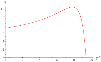
Figure 28: The $p^{2}$ dependence of $g=g_{JDD}(m_{D}^{2},\,m^{2}_{D},\,p^{2})$, showing the almost complete cancellation between the pole of $\xi(\omega)$ and the kinematic zero. The units of $p^{2}$ are GeV².

For $0<p^{2}<4$ GeV², $g_{JDD}$ is almost constant,

$$g_{JDD}=8.0\pm 0.5\ .$$ (29)

For larger values of $p^{2}$ the method is unreliable due to the incomplete cancellation between the kinematical zero and the pole. The distorted shape around the $J/\psi$ pole suggests that the contribution of the nearby $\psi(2S)$ pole could also be relevant. Therefore, we extrapolate the smooth behavior of $g_{JDD}$ in the small $p^{2}$ region up to $p^{2}=m^{2}_{J/\psi}$ and assume the value of $g_{JDD}$ in Eq. (29) for on-shell $J/\psi$. On the other hand, the behavior with $p_{1}^{2}$ and $p^{2}_{2}$ is smooth, compatible with that of a smooth form factor. We finally note that Eq. (29) agrees with the result of the QCD sum rule analysis [128, 129]. This is not surprising since QCD sum rules involve a perturbative part and a suppressed nonperturbative contribution. The perturbative term has its counterpart in the CQM loop calculation of Fig. 27 with an overall normalization that should agree with the CQM as a consequence of Luke’s theorem.

We now turn to the $JD^{(*)}D^{(*)}\pi$ couplings. As discussed in Refs. [126, 134], the leading contributions to the current matrix element, $\langle H(v^{\prime})\pi|\overline{c}\gamma^{\mu}c|H(v)\rangle$, in the soft pion limit (SPL) are the pole diagrams. Technically, in the SPL, the reducing action of a pion derivative in the matrix element is compensated in the polar diagrams by the effect of the vanishing denominator in the combined $q_{\pi}\rightarrow 0,\,m_{c}\rightarrow\infty$ limit. Since the effect of the pole diagrams is explicitly taken account in Fig. 26, we do not include any further contributions. To be definite, we consider the coupling $g_{JDD\pi}$ which can be obtained by a VMD ansatz similar to Fig. 27. Now the left-hand side is modified by the insertion of a soft pion on the light quark line with the coupling $q_{\pi}^{\mu}/f_{\pi}\gamma_{\mu}\gamma_{5}$. We call $\xi^{\pi}(\omega)$ the analogous form factor in the SPL,

$$\xi^{\pi}(\omega)=Z_{H}\left[\frac{4m+2\Delta_{H}}{1+\omega}I_{4}(\Delta_{H})-\left(m^{2}+\frac{2\Delta_{H}^{2}+4m\Delta_{H}}{1+\omega}\right)\frac{\partial I_{5}(\Delta_{H},\Delta_{H},\omega)}{\partial m^{2}}\right]\,\,.$$ (30)

The VMD ansatz of Fig. 27 gives

$${\cal L}_{JDD\pi}=ig_{JDD\pi}\epsilon^{\mu\nu\alpha\beta}J_{\mu}\partial_{\nu}D\partial_{\alpha}\overline{D}\partial_{\beta}\pi$$ (31)

with

$$g_{JDD\pi}(p_{1}^{2},\,p_{2}^{2},\,p^{2})=\frac{(m_{J}^{2}-p^{2})\xi^{\pi}(\omega)}{f_{\pi}f_{J}m_{D}m_{J}}\,\,.$$ (32)

In Fig. 29 we plot our result for $g_{JDD\pi}$ with on-shell $D$ mesons.

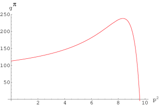
Figure 29: The $p^{2}$ dependence of $g^{\pi}=g_{JDD\pi}(m_{D}^{2},\,m^{2}_{D},\,p^{2})$. As in Fig. 28 there is an almost complete cancellation between the pole of the form factor and the kinematic zero. The units on $p^{2}$ are GeV² and GeV^-3 for $g_{JDD\pi}$.

By the same arguments used to determine $g_{JDD}$, we find, with all mesons on mass-shell,

$$g_{JDD\pi}=125\pm 15~{}{\rm GeV}^{-3}\,\,.$$ (33)

We now compare this result with the effective $JDD\pi$ coupling obtained by a polar diagram with an intermediate $D^{*}$ state. In this case,

$$g_{JDD\pi}^{\rm polar}\approx\frac{(g_{JDD^{*}})(g_{D^{*}D\pi})}{2q_{\pi}\cdot p_{D}}\ \,.$$ (34)

Since all the calculations are valid in the SPL, only pion momenta of up to a few hundred MeV should be considered. Using the result $g_{D^{*}D\pi}=2m_{D}/f_{\pi}g$, with $g=0.59\pm 0.01\pm 0.07$ [127], we find $g_{JDD\pi}^{\rm polar}\approx 393$, 196, and 98 GeV^-3 for $|q_{\pi}|=50$, 100, and 200 MeV respectively. This analysis shows that, within the region of validity of the model, in spite of the rather large value of the coupling in Eq. (33), the diagrams containing this coupling are in general suppressed. Similar conclusions are reached for $D^{*}$’s.

Finally, we discuss the kinematical limits of our approach. To allow the production of a $D^{(*)}\overline{D}^{(*)}$ pair, as shown in Fig. 26, we must extend the region of validity of the model beyond the SPL since the $D^{(*)}\overline{D}^{(*)}$ threshold is $|\vec{q}_{\pi}|=700-1000~{}$MeV. The CQM, along with other models, is a chiral model which puts limits on the pion momenta. Therefore it is necessary to include a form factor enhancing the small pion momenta region, for example

$$f(|\vec{q}_{\pi}|)=\frac{1}{1+(|\vec{q}_{\pi}|/m_{\chi})}\,\,.$$ (35)

A similar form factor is considered in Ref. [120] but with a different motivation. Here we introduce it to ensure the validity of our approach. In this sense, the cross sections we can compute may be considered as lower bounds. Since the main effect of Eq. (35) should be to reduce contributions from pion momenta larger than a few hundred MeV, we expect $400<m_{\chi}<600$ MeV. This choice implies that the direct couplings in Fig. 26, diagrams 1c, 2d and 3e, should not dominate the final result since their contribution is larger where the form factor is more effective.

4.2.1 Definitions of the integrals

We list the expressions used to compute the integrals $I_{i}$ used in the text. The ultraviolet cutoff $\Lambda$, the infrared cutoff, $\mu$, and the light constituent mass, $m$, are $\Lambda=1.25$ GeV, $\mu=0.3$ GeV and $m=0.3$ GeV [130, 131].

$$I_{3}(\Delta) = -\frac{iN_{c}}{16\pi^{4}}\int^{\mathrm{reg}}\frac{d^{4}k}{(k^{2}-m^{2})(v\cdot k+\Delta+i\epsilon)}$$ (36)

$$= {N_{c}\over{16\,{{\pi}^{{3/2}}}}}\int_{1/{{\Lambda}^{2}}}^{1/{{\mu}^{2}}}{ds\over{s^{3/2}}}\;e^{-s({m^{2}}-{{\Delta}^{2}})}\;[1+{\mathrm{erf}}(\Delta\sqrt{s})]$$

$$I_{4}(\Delta) = \frac{iN_{c}}{16\pi^{4}}\int^{\mathrm{reg}}\frac{d^{4}k}{(k^{2}-m^{2})^{2}(v\cdot k+\Delta+i\epsilon)}$$ (37)

$$= \frac{N_{c}}{16\pi^{3/2}}\int_{1/\Lambda^{2}}^{1/\mu^{2}}\frac{ds}{s^{1/2}}\;e^{-s(m^{2}-\Delta^{2})}\;[1+{\mathrm{erf}}(\Delta\sqrt{s})]$$

$$I_{5}(\Delta_{1},\Delta_{2},\omega) = \frac{iN_{c}}{16\pi^{4}}\int^{\mathrm{reg}}\frac{d^{4}k}{(k^{2}-m^{2})(v\cdot k+\Delta_{1}+i\epsilon)(v^{\prime}\cdot k+\Delta_{2}+i\epsilon)}$$ (38)

$$= \int_{0}^{1}dx\frac{1}{1+2x^{2}(1-\omega)+2x(\omega-1)}$$

$$\times\Big{[}\frac{6}{16\pi^{3/2}}\int_{1/\Lambda^{2}}^{1/\mu^{2}}ds~{}\sigma_{\Delta}\;e^{-s(m^{2}-\sigma_{\Delta}^{2})}\;s^{-1/2}\;[1+{\mathrm{erf}}(\sigma_{\Delta}\sqrt{s})]$$

$$+\frac{6}{16\pi^{2}}\int_{1/\Lambda^{2}}^{1/\mu^{2}}ds\;e^{-s\sigma_{\Delta}^{2}}\;s^{-1}\Big{]}\,\,,$$

where

$$\sigma_{\Delta}\equiv\sigma(x,\Delta_{1},\Delta_{2},\omega)={{{\Delta_{1}}\,\left(1-x\right)+{\Delta_{2}}\,x}\over{{\sqrt{1+2\,\left(\omega-1\right)\,x+2\,\left(1-\omega\right)\,{x^{2}}}}}}\,\,.$$ (39)

4.3 Heavy Quark Energy Loss in QCD Matter 

The study of heavy quark production in nuclear collisions will allow extraction of valuable information on the gluon densities of the colliding nuclei. In addition, since the heavy quarks propagate through the quark–gluon matter created in such collisions, they can be used to probe the properties of the dense matter. The practical importance of heavy quark energy loss to the charmed hadron and lepton spectra has been clearly established [135, 136, 137, 138, 139].

The idea of heavy quark energy loss has attracted considerable attention. In particular, collisional energy loss in quark–gluon plasma has been evaluated [140, 141, 142] using finite–temperature QCD, see Ref. [143] for a comprehensive review. However, the energy loss of fast partons in medium is dominated by gluon radiation [144, 145, 146]. Radiative energy loss by heavy quarks was evaluated in Ref. [147]. It was shown [147] that the “dead cone effect” in the radiation of a heavy quark significantly suppresses its energy loss while making the calculation more reliable by reducing the sensitivity to the infrared region.

In fact, the first measurements of charm production in Au+Au collisions at RHIC [148, 149] indicated very small, if any, nuclear effect on the shape of charm transverse momentum distributions. The smaller loss predicted in Ref. [147] provides a plausible and economical explanation of the observed phenomenon [150, 151]. The “dead cone” effect has been taken into account in the studies of charm and bottom production at the LHC [152].

In the following we give a brief and qualitative explanation of the results of Ref. [147]. We first recall the basic features of gluon radiation caused by propagation of a fast parton (quark) through a QCD medium.

As pointed out in Ref. [145], the accompanying radiation is determined by multiple rescattering of the radiated gluon in the medium. The gluon, during its formation time,

$$t_{\rm form}\simeq\frac{\omega}{k_{T}^{2}}\,,$$ (40)

accumulates a typical transverse momentum

$$k_{T}^{2}\simeq\mu^{2}\ {t_{\rm form}\over\lambda},$$ (41)

where $\lambda$ is the mean free path and $\mu^{2}$ the characteristic momentum transfer squared in a single scattering. This is the random walk pattern with an average number of scatterings given by $t_{\rm form}/\lambda$.

Combining Eqs. (40) and (41) we obtain

$$N_{\rm coh}=\frac{t_{\rm form}}{\lambda}=\sqrt{\frac{\omega}{\mu^{2}\,\lambda}}\,,$$ (42)

the number of scattering centres which participate, coherently, in the emission of the gluon with a given energy $\omega$. For sufficiently large gluon energies, $\omega>\mu^{2}\lambda$, when the coherent length exceeds the mean free path, $N_{\rm coh}>1$. In this situation, the standard Bethe-Heitler energy spectrum per unit length describing independent emission of gluons at each scattering centre is suppressed:

$$\frac{dW}{d\omega dz}=\frac{1}{N_{\rm coh}}\left(\frac{dW}{d\omega dz}\right)^{\rm BH}=\frac{\alpha_{s}C_{R}}{\pi\omega\,\lambda}\sqrt{\frac{\mu^{2}\,\lambda}{\omega}}=\frac{\alpha_{s}C_{R}}{\pi\omega}\sqrt{\frac{\hat{q}}{\omega}}\,\,.$$ (43)

Here $C_{R}$ is the “colour charge” of the parton projectile ($C_{R}=C_{F}=(N_{c}^{2}-1)/2N_{c}=4/3$ for quarks).

In Eq. (43) we have substituted the characteristic ratio $\mu^{2}/\lambda$ by the gluon transport coefficient [153],

$$\hat{q}\equiv\rho\ \int{d\sigma\over dq^{2}}\ q^{2}\ dq^{2}\,\,,$$ (44)

proportional to the density $\rho$ of the scattering centres in the medium. The transport coefficient characterizes the typical momentum transfer in gluon scatterings off these centres.

An important feature of medium-induced radiation is the relation between the transverse momentum and the energy of the emitted gluon. Indeed, from Eqs. (40) and (41), see also Eq. (44), we derive

$$k_{T}^{2}\simeq\sqrt{\hat{q}\ \omega}\,\,.$$ (45)

Thus the angular distribution of gluons with a given energy $\omega$ is concentrated at a characteristic energy- and medium- dependent emission angle,

$$\theta\simeq\frac{k_{T}}{\omega}\sim\left(\frac{\hat{q}}{\omega^{3}}\right)^{1/4}.$$ (46)

Gluon bremsstrahlung off a heavy quark differs from the case of a massless parton produced at the same hardness scale in one respect: gluon radiation is suppressed at angles smaller than the ratio of the quark mass $m_{Q}$ to its energy $E$. Indeed, the distribution of soft gluons radiated by a heavy quark is given by

$$dP_{\rm HQ}={\alpha_{s}\ C_{F}\over\pi}\ {d\omega\over\omega}\ {k_{T}^{2}\,dk_{T}^{2}\over(k_{T}^{2}+\omega^{2}\theta_{0}^{2})^{2}}\,\,,\qquad\theta_{0}\equiv\frac{m_{Q}}{E}\,\,,$$ (47)

where the strong coupling constant $\alpha_{s}$ should be evaluated at the scale determined by the denominator of Eq. (47). Equating $k_{T}$ with $\omega\theta$ in the small-angle approximation, we conclude that Eq. (47) differs from the standard bremsstrahlung spectrum,

$$dP_{0}\>\simeq\>\frac{\alpha_{s}\,C_{F}}{\pi}\frac{d\omega}{\omega}\,\frac{dk_{T}^{2}}{k_{T}^{2}}\>=\>\frac{\alpha_{s}\,C_{F}}{\pi}\frac{d\omega}{\omega}\,\frac{d\theta^{2}}{\theta^{2}}\,\,,$$ (48)

by the factor

$$dP_{\rm HQ}=dP_{0}\left(1+\frac{\theta_{0}^{2}}{\theta^{2}}\right)^{-2}\,\,.$$ (49)

This effect is known as the “dead cone” phenomenon. Suppression of small-angle radiation has a number of interesting implications, such as the perturbative calculability of, and nonperturbative $\Lambda/m_{Q}$ corrections to, heavy quark fragmentation functions [154, 155], multiplicity and energy spectra of light particles accompanying hard production of a heavy quark [156, 157].

In the present context we should compare the angular distribution of gluons induced by the quark propagation in the medium with the size of the dead cone. To this end, for the sake of a semi-quantitative estimate, we substitute the characteristic angle, Eq. (46), into the dead cone suppression factor, Eq. (49), and combine it with the radiation spectrum, Eq. (43), to arrive at

$$I(\omega)=\omega{dW\over d\omega}={\alpha_{s}\ C_{F}\over\pi}\sqrt{{\omega_{1}\over\omega}}\ {1\over(1+(\ell\,\omega)^{3/2})^{2}}\,\,,$$ (50)

where

$$\ell\equiv\hat{q}^{-1/3}\ \left({m_{Q}\over E}\right)^{4/3}.$$ (51)

To determine whether the finite quark mass essentially affects the medium-induced gluon yield, we need to estimate the product $\ell\omega$ for the maximum gluon energy, $\omega\simeq\omega_{1}$, achievable in Eq. (43),

$$\ell\omega_{1}=\hat{q}^{-1/3}\ \left({m_{Q}\over E}\right)^{4/3}\hat{q}L^{2}=\left(\frac{E_{\rm HQ}}{E}\right)^{4/3}\,,\qquad E_{\rm HQ}\equiv m_{Q}\sqrt{\hat{q}L^{3}}\,\,.$$ (52)

where $L$ is the path length through the medium. Thus the quark mass becomes irrelevant when its energy exceeds the characteristic value, $E_{\rm HQ}$, dependent on the size of the medium and on its “scattering power” embodied in the transport coefficient $\hat{q}$.

Which regime is realized in the experiments on heavy quark production in nuclear collisions? Taking $m_{c}=1.5$ GeV, we estimate [147]

$$E_{\rm HQ}^{\rm cold} = \sqrt{\hat{q}_{\rm cold}}\ L^{3/2}\ m_{c}\simeq\ 20\,{\rm GeV}\left({L\over 5\,{\rm fm}}\right)^{3/2}\,,$$ (53)

$$E_{\rm HQ}^{\rm hot} = \sqrt{\hat{q}_{\rm hot}}\ L^{3/2}\ m_{c}\simeq\ 92\,{\rm GeV}\left({L\over 5\,{\rm fm}}\right)^{3/2},$$ (54)

for cold and hot matter, respectively. We observe that, in practice, $E\ll E_{\rm HQ}$ for the transverse momentum (energy) distributions of heavy mesons, especially in the hot medium. We thus conclude that the pattern of medium-induced gluon radiation appears to be qualitatively different for heavy and light quarks in the kinematic region of interest.

The issue of in-medium quenching of inclusive particle spectra was addressed in Ref. [158]. The $p_{T}$ spectrum is given by the convolution of the transverse momentum distribution in an elementary hadron–hadron collision, evaluated at a shifted value $p_{T}+\epsilon$, with the distribution $D(\epsilon)$ in the energy $\epsilon$ lost by the quark to the medium-induced gluon radiation:

$${d\sigma^{\rm med}\over dp_{T}^{2}}=\int d\epsilon\ D(\epsilon)\ {d\sigma^{\rm vac}(p_{T}+\epsilon)\over dp_{T}^{2}}\equiv{d\sigma^{\rm vac}(p_{T})\over dp_{T}^{2}}\,Q(p_{T}),$$ (55)

where $Q(p_{T})$ is a medium-dependent quenching factor. Because in the region of interest, $\epsilon\ll p_{T}$, when the vacuum cross section is a steeply-falling function, the calculation of the quenching factor $Q$ can be simplified by approximating the $\epsilon$-integral in Eq. (55) as an exponential,

$$Q(p_{T})\simeq\int d\epsilon\ D(\epsilon)\ \exp\left\{\frac{\epsilon}{p_{T}}{\cal{L}}\right\}\,\,,\qquad{\cal{L}}\equiv\frac{d}{d\ln p_{T}}\ln\left[{d\sigma^{\rm vac}(p_{T})\over dp_{T}^{2}}\right]\,\,.$$ (56)

Figure 30: The ratio of quenching factors $Q_{H}(p_{T})/Q_{L}(p_{T})$ for charm and light quarks in cold nuclear matter with $\hat{q}=0.01$ GeV³ and $L=5$ fm. From Ref. [147].

According to Eq. (54), we expect a larger quenching ratio for a hot medium. Indeed, the $D/\pi$ ratio should become significantly enhanced relative to $pp$ collisions. Assuming a fixed path length traversed by the quarks in the hot medium, $L=5$ fm, we find a factor of $\sim 2$ enhancement at $p_{T}\sim 5-10$ GeV.

The following result for the heavy quark quenching factor was derived in Ref. [147]:

$$Q_{H}(p_{T})\simeq\exp\left[-{2\alpha_{s}C_{F}\over\sqrt{\pi}}\ L\,\sqrt{\hat{q}\frac{{\cal{L}}_{H}}{p_{T}}}\,+\,{16\alpha_{s}C_{F}\over 9\sqrt{3}}L\left(\frac{\hat{q}\>\>m_{Q}^{2}}{m_{Q}^{2}+p_{T}^{2}}\right)^{1/3}\right]\,\,.$$ (57)

The first term in the exponent in Eq. (57) represents the quenching of the transverse momentum spectrum, universal for light and heavy quarks,

$$Q_{L}(p_{T})\simeq\exp\left[-{2\alpha_{s}C_{F}\over\sqrt{\pi}}\ L\,\sqrt{\hat{q}\frac{{\cal{L}}_{L}}{p_{T}}}\,\right]$$

modulo the difference in ${\cal{L}}$ determined by the vacuum $p_{T}$ distributions. The second term in Eq. (57) is specific to heavy quarks. It has a positive sign so that the suppression of the heavy hadron $p_{T}$ distributions is always smaller than that of the light hadrons. This is a straightforward consequence of the fact that the heavy quark mass suppresses gluon radiation. At very high transverse momenta both terms vanish in accord with the QCD factorization theorem which states that medium effects should disappear as $p_{T}\rightarrow\infty$. How fast this regime is approached depends, however, on the properties of the medium encoded in the transport coefficient $\hat{q}$ and the path length $L$.

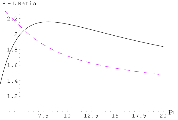
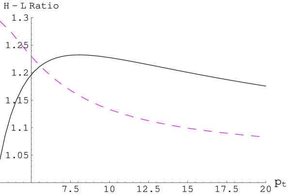
Figure 31: The ratio of quenching factors $Q_{H}(p_{T})/Q_{L}(p_{T})$ for charm and light quarks in hot matter with $\hat{q}=0.2$ GeV³ ($L=5$ fm upper panel, $L=2$ fm lower panel). Solid lines correspond to unrestricted gluon radiation, while the dashed lines are based on the calculation with the cut $\omega>0.5$ GeV on gluon energies. From Ref. [147].

Constructing the ratio $Q_{H}$ to $Q_{L}$, the heavy-to-light quenching should be enhanced by

$$\frac{Q_{H}(p_{T})}{Q_{L}(p_{T})}\>\simeq\>\exp\left[{16\alpha_{s}C_{F}\over 9\sqrt{3}}L\left(\frac{\hat{q}\>\>m_{Q}^{2}}{m_{Q}^{2}+p_{T}^{2}}\right)^{1/3}\right]\,\,.$$ (58)

This simple expression provides a reasonably good approximation to the more accurate quantitative results presented in Ref. [147].

As discussed above, the quenching of heavy hadron $p_{T}$ distributions caused by QCD matter is much weaker than for pions because the gluon cloud around the heavy quark is “truncated” by the large quark mass in a medium-dependent way. This interesting effect can be illustrated by the transverse momentum dependence of the ratio of hadrons originating from heavy and light quark fragmentation such as the $D/\pi$ ratio in heavy ion collisions.

Fig. 30 shows the ratio of quenching factors, Eq. (58), for heavy and light quarks in cold nuclear matter, $L=5$ fm, relevant to high-$p_{T}$ particle production in $pA$ collisions. A small value of the transport coefficient, $\hat{q}_{\rm cold}\simeq 0.01$ GeV³, translates into a $\sim$ 15% enhancement, reduced to $\approx 1$% for $L=2$ fm.

We only present the ratio of quenching factors because, as pointed out in Ref. [158], the absolute magnitude of the quenching turns out to be extremely sensitive to gluon radiation in the few-hundred MeV energy range. Thus the magnitude cannot be quantitatively predicted without a detailed understanding of the spectral properties of the medium.

The heavy-to-light ratio, however, proves to be much less sensitive to the infrared region since gluon radiation off heavy and light quarks is universal in the $x\rightarrow 0$ limit, see Eq. (50). To illustrate this point, in Fig. 31 we show the ratio of quenching factors calculated with the gluon energies restricted to $\omega>500$ MeV. We see that, in the $5-10$ GeV range of $p_{T}$, the ratio is modified by $20-30$ %.

Clearly, detailed calculations have to be performed before a reliable estimate of the magnitude of the $D/\pi$ enhancement can be presented. Nevertheless, the $D/\pi$ and $B/\pi$ ratios appear to be extremely sensitive to the density of colour charges in QCD matter. Of special interest is the $B/D$ ratio, for which these calculations become even less sensitive to the infrared region and thus more stable.

5 QUARKONIUM FORMATION FROM UNCORRELATED QUARK-ANTIQUARK PAIRS 

5.1 Introduction

The goal of this section is to assess the possibility that quarkonium production rates may be enhanced in nucleus-nucleus interactions at the LHC relative to that predicted by extrapolation of processes thought to be dominant at lower energy. This enhancement could follow from the effects of incoherent recombination mechanisms involving uncorrelated pairs of heavy quarks and antiquarks which result from multiple pair production. Two different approaches have been considered: statistical hadronization and kinetic formation. Updated predictions relevant to Pb+Pb collisions at the LHC are given.

The utility of heavy quarkonium production rates in nuclear collisions as a signature of color deconfinement was proposed more than 15 years ago [1]. Since one expects that the long-range color confining potential will be screened in a deconfined medium, the quark and antiquark constituents of bound states will be liberated. As the system expands and cools, these constituents will, in general, diffuse away from each other to separations larger than typical hadronic dimensions. When the confining potential reappears, a given heavy quark will not be able to “find” its heavy antiquark partner and form heavy quarkonium. It must then bind with one of the antiquarks within range at hadronization. Since these antiquarks are predominantly the lighter $u$, $d$, and $s$ flavors, the final hadronic states will preferentially be those with “open” heavy flavor. The result will be a decreased population of heavy quarkonium relative to that which would have formed if a region of deconfinement had not been present. This scenario as applied to the charm sector is known as $J/\psi$ suppression.

At LHC energy, perturbative QCD estimates predict that hundreds of pairs of charm-anticharm quarks will be produced in a central lead-lead collision. This situation provides a “loophole” in the Matsui-Satz argument [1] since there will be copious numbers of heavy antiquarks in the interaction region with which any given heavy quark may combine. In order for this to happen, however, one must invoke a physical situation in which quarkonium states can be formed from all combinations of heavy quarks and antiquarks. This of course would be expected to be valid in the case that a space-time region of color deconfinement is present, but it is not necessarily limited to this possibility.

One can make a model-independent estimate of how such a “recombination” mechanism would depend on nuclear collision observables. For a given charm quark, the probability $\cal{P}$ to form a $J/\psi$ is proportional to the number of available anticharm quarks relative to the number of light antiquarks,

$${\cal{P}}\propto\frac{N_{\overline{c}}}{N_{\overline{u},\overline{d},\overline{s}}}\propto\frac{N_{c\overline{c}}}{N_{\rm ch}}\,\,.$$ (59)

In the second step, we have replaced the number of available anticharm quarks by the total number of pairs initially produced, assuming that the total number of bound states formed remains a small fraction of the total $c\overline{c}$ production. We normalize the number of light antiquarks by the number of produced charged hadrons. Since this probability is generally very small, one can simply multiply by the total number of charm quarks, $N_{c}$, to obtain the number of $J/\psi$ expected in a given event,

$$N_{J/\psi}\propto\frac{{N_{c\overline{c}}}^{2}}{N_{\rm ch}}\,\,,$$ (60)

where the use of the initial values $N_{c\overline{c}}=N_{c}=N_{\overline{c}}$ is again justified by the relatively small number of bound states formed.

The essential property of this result is that the growth of $N_{J/\psi}$, quadratic in the total number of charm quarks, with energy [159] is expected to be much faster than the growth of total particle production in heavy ion collisions [160]. Without this quadratic mechanism, $J/\psi$ production is typically some small energy-independent fraction of total initial charm production [20]. We thus anticipate that the quadratic formation will become dominant at sufficiently high energy. Generic estimates of the significance of this type of formation process can be made [161]. Here we look at specific predictions of two models – statistical hadronization and kinetic formation, considered in sects. 5.2 and 5.3 respectively – which share the above properties, and we update the expectations to LHC energies.

5.2 Statistical Hadronization

The statistical hadronization model is motivated by the successful fits of relative abundances of light hadrons produced in high energy heavy ion interactions according to a hadron gas in chemical and thermal equilibrium [162]. Extension of the model to hadrons containing heavy quarks underpredicts the observed abundances. This effect may be attributed to the long time scales associated with thermal production and annihilation of heavy quarks. The statistical hadronization model as first formulated for charm quarks [163] assumes that the $c\overline{c}$ pairs produced in the initial hadronic interactions survive until their subsequent hadronization, at which time they are distributed into hadrons according to the same thermal equilibrium parameters that fit the light hadron abundances. Chemical equilibrium abundances are adjusted by a factor $\gamma_{c}$ which accounts for the non-thermal heavy quark density. One power of this factor multiplies a given thermal hadron population for each heavy quark or antiquark contained in the hadron. Thus the relative abundance of the $J/\psi$ to that of $D$ mesons, for example, may be enhanced in this model.

The value of $\gamma_{c}$ is determined by conservation of the heavy quark flavor. For the charm sector, the conservation constraint relates the number of initially-produced $c\bar{c}$ pairs $N_{c\overline{c}}$ to their distribution into open and hidden charm hadrons,

$$N_{c\overline{c}}={1\over 2}\gamma_{c}N_{\rm open}+{\gamma_{c}}^{2}N_{\rm hidden},$$ (61)

where $N_{\rm open}$ is the number of hadrons containing one $c$ or $\overline{c}$ quark and $N_{\rm hidden}$ is the number of hadrons containing a $c\overline{c}$ pair. For most applications, $N_{\rm hidden}$ (and also multi-charm hadrons) can be neglected compared with $N_{\rm open}$ due to the mass differences. Thus the charm enhancement factor is simply

$$\gamma_{c}={2N_{c\overline{c}}\over N_{\rm open}},$$ (62)

leading directly to the quadratic dependence of the hidden charm hadron population on $N_{c\overline{c}}$. One can then express the total number of $J/\psi$ in terms of the various thermal densities, $n_{i}$, and the total number of $c\overline{c}$ pairs, $N_{c\overline{c}}$. One factor of system volume $V$ remains implicit here. It is generally replaced by the ratio of number to density for total charged hadrons, $n_{\rm ch}/N_{\rm ch}$. Then the number of $J/\psi$ produced obeys the generic form anticipated in Eq. (60).

$$N_{J/\psi}=4{n_{\rm ch}n_{J/\psi}\over{n_{\rm open}}^{2}}{N_{c\overline{c}}^{2}\over N_{\rm ch}}$$ (63)

For collider experiments such as those at the LHC and RHIC, relating the corresponding central rapidity densities will be more relevant. Since Eq. (63) is homogeneous in the total particle and quark pair numbers, it will also be valid if these are replaced by their rapidity densities. To get an order of magnitude estimate, we choose a “standard” set of thermal parameters, $T=170$ MeV and $\mu_{B}\approx 0$, for which the thermal density ratio is approximately $0.5$. For a specific normalization, we assume $dN_{\rm ch}/dy$ = 2000 for a central collision at the LHC and take the initial charm rapidity density to be $dN_{c\overline{c}}/dy=25$, roughly corresponding to $N_{c\overline{c}}=200$ for central collisions $(b=0)$. Using these inputs, one predicts $dN_{J/\psi}/dy=0.625$, indicating that several $J/\psi$ will form through statistical hadronization in a central collision. To put this number in perspective, it is revealing to form the $J/\psi$ to $N_{c\overline{c}}$ rapidity density ratio, 0.025 with the same assumptions. For comparison, one expects the corresponding hadronic production ratio to be of $0.01$. This number would then be significantly reduced if placed in a region of color deconfinement. Thus the efficiency of $J/\psi$ formation via statistical hadronization at the LHC is expected to be substantial.

These numbers can be easily adjusted to other charm and charged particle densities using Eq. (63). Variations of the thermal parameters can also be investigated. For example, if the hadronization temperature is decreased to 150 MeV, the prefactor combination of thermal densities increases by approximately a factor of two.

The centrality dependence is controlled by the behavior of $N_{c\overline{c}}$ and $N_{\rm ch}$. The former should be proportional to the nuclear overlap function $T_{AA}(b)$ but is generally recast in terms of the dependence on the number of nucleon participants, $N_{\rm part}$. The calculation of $N_{\rm part}$ requires a model calculation dependent on the total inelastic cross section, $\sigma_{\rm in}$, as well as the nuclear geometry. We parameterize the expected behavior as a power-law $N_{c\overline{c}}\propto{N_{\rm part}}^{4/3}$. However, there will be deviations from this behavior for the larger values of $\sigma_{\rm in}$ expected at the LHC [164]. The centrality dependence of $N_{\rm ch}$ at RHIC is also consistent with a power-law with exponent $\approx$ 1.2 [160, 165]. We will use the same dependence for our estimates at the LHC. It is clear that for sufficiently peripheral collisions one will encounter situations in which the average number of initially produced $c\overline{c}$ pairs is of order unity or less. At this point, one must revisit the assumptions of the original statistical hadronization model which assumed a grand canonical ensemble. The grand canonical approach is valid only when $N_{c\overline{c}}$ is large enough for the fluctuations about the average value to be negligible. Thus for peripheral collisions, one must recalculate the statistical results in the canonical approach where the charm number is exactly conserved, as noted in [166]. Charm conservation can be implemented via a correction factor [167],

$$N_{c\overline{c}}={1\over 2}\gamma_{c}N_{\rm open}{{I_{1}(\gamma_{c}N_{\rm open})}\over{I_{0}(\gamma_{c}N_{\rm open})}}+{\gamma_{c}}^{2}N_{\rm hidden}.$$ (64)

In the limit of large $\gamma_{c}N_{\rm open}$, the ratio of Bessel functions $I_{i}$ approaches unity and the grand canonical result is recovered. In the opposite limit when $\gamma_{c}N_{\rm open}\rightarrow 0$, the ratio of Bessel functions approaches ${1\over 2}\gamma_{c}N_{\rm open}$. In this limit, the dependence on $N_{c\overline{c}}$ in Eq. (63) changes from quadratic to linear. At the LHC this effect will not be relevant until one reaches very peripheral events, but at lower energies it can be significant over a much larger range of centralities [168].

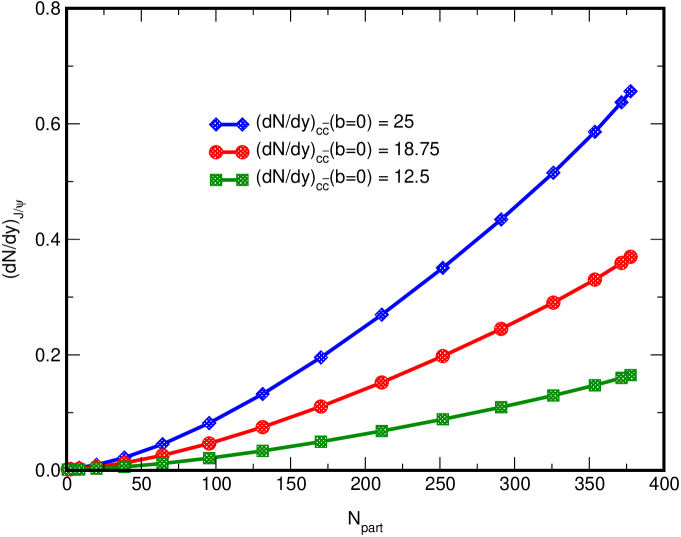
Figure 32: Statistical hadronization results for $J/\psi$ production as a function of $N_{\rm part}$ at the LHC.

The results for $dN_{J/\psi}/dy$ as a function of $N_{\rm part}$ at the LHC are shown in Fig. 32. The results are shown for three different values of $dN_{c\overline{c}}/dy(b=0)$, corresponding to $N_{c\overline{c}}(0)\approx 200$, 150, and 100. There is a rapid increase with centrality due to the quadratic dependence of $N_{J/\psi}$ on $N_{c\overline{c}}$.

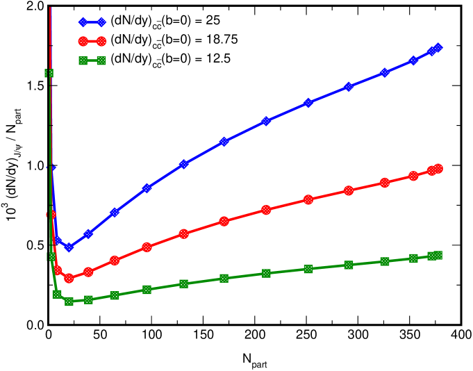
Figure 33: The statistical hadronization results of Fig. 32 divided by $N_{\rm part}$ as a function of $N_{\rm part}$.

It is also interesting to look at these results normalized by $N_{\rm part}$, shown in Fig. 33. This ratio also increases with centrality, providing a signature for the statistical hadronization process that is less dependent on $N_{c\overline{c}}$ for the overall normalization. The corresponding results when normalized by $dN_{c\overline{c}}/dy$ are shown in Fig. 34. The same general behavior is seen but the increase with centrality is less pronounced since the $dN_{c\overline{c}}/dy$ is assumed to vary with a larger power, ${N_{\rm part}}^{4/3}$. All of these ratios are at the percent level for central collisions and hence are larger than expected if the total $J/\psi$ population were due to initial production followed by suppression in a deconfined medium.

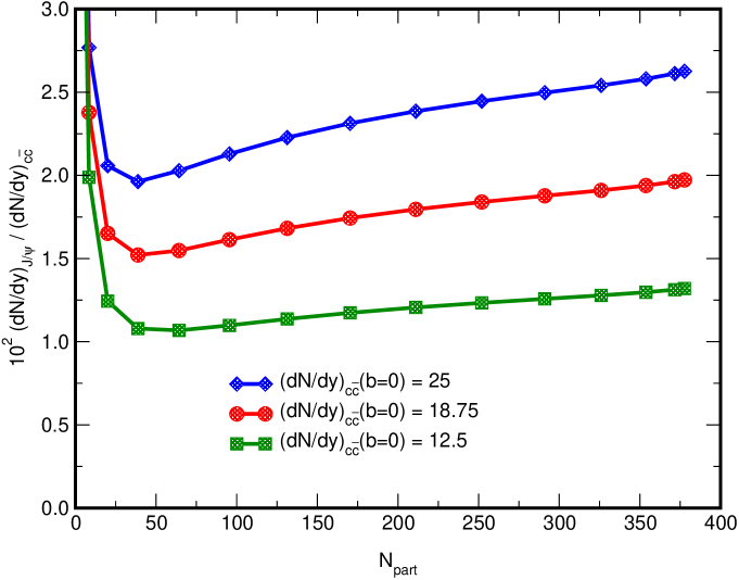
Figure 34: The statistical hadronization results for $J/\psi$ production at the LHC, divided by the open charm multiplicity, $dN_{c\overline{c}}/dy$, as a function of $N_{\rm part}$.

The region of very peripheral collisions deserves some separate comments. First, there is a rise at low $N_{\rm part}$ in both Figs. 33 and 34 due to the onset of corrections from the canonical ensemble treatment. However, the extremely large values of the ratios as $N_{\rm part}\rightarrow 0$ are an artifact of the decreasing interaction volume, $V\rightarrow 0$. This calculation must be cut off before $N_{\rm part}=2$, i.e. only one interacting pair. It is also in this region where one must take into account the remaining $J/\psi$ from initial production. Since the survival probability is maximum for very peripheral collisions and the statistical hadronization process is least effective in this same region, there will be a crossover in the relative importance of the two mechanisms. Some studies have already been performed for this situation at SPS and RHIC energies [169, 170, 171].

Finally, there is another lower cutoff in centrality for the statistical hadronization results, needed to avoid a contradiction with the $\psi\prime/(J/\psi)$ ratio at the SPS. Since both of these states receive identical factors of $\gamma_{c}$, their ratio must be that predicted for chemical equilibrium in the absence of any charm enhancement or suppression. Although the measured ratio appears to be consistent for more central collisions [172], there is an indication that it rises sharply for more peripheral collisions. Most treatments have thus inserted a cutoff of $N_{\rm part}$ = 100, below which model predictions become inconsistent [163].

The numerical values for $dN_{J/\psi}/dy$ are tabulated as a function of impact parameter in Table 17 for the three choices of initial charm multiplicity density and the default values of all other quantities.

5.3 Kinetic Formation in a Deconfined Region

The kinetic model has been developed [173, 174] to investigate the possibility that $J/\psi$ may form directly in a deconfined medium. This formation takes advantage of the mobility of the initially-produced charm quarks in a deconfined region. In order to motivate this view, consider the “standard” physical picture of deconfinement in which quarkonium is suppressed by collisions with free gluons in the medium [175]. Then the formation process, in which a $c$ and $\overline{c}$ in a relative color octet state are captured into a color-singlet quarkonium bound state and emit a color octet gluon, is simply the inverse of the the breakup reaction responsible for the suppression. This is an inevitable consequence of the suppression picture.

The proper time evolution of the $J/\psi$ population is given by the rate equation

$$\frac{dN_{J/\psi}}{d\tau}=\lambda_{\mathrm{F}}\frac{N_{c}\,N_{\overline{c}}}{V(\tau)}-\lambda_{\mathrm{D}}N_{J/\psi}\,\rho_{g}\,\,,$$ (65)

where $\rho_{g}$ is the gluon number density and $V(\tau)$ is the time-dependent volume of the deconfined spatial region. The reactivities $\lambda_{\rm F,D}$ are the reaction rates, $\langle\sigma v_{\mathrm{rel}}\rangle$, averaged over the momentum distributions of the initial participants, i.e. $c$ and $\overline{c}$ for $\lambda_{\rm F}$ and $J/\psi$ and $g$ for $\lambda_{\rm D}$.

The solution of Eq. (65) grows quadratically with $N_{c\overline{c}}$, as long as $N_{J/\psi}\ll N_{c\overline{c}}$. In this case, we have

$$N_{J/\psi}(\tau_{f})=\epsilon(\tau_{f})\left[N_{J/\psi}(\tau_{0})+N_{c\overline{c}}^{2}\int_{\tau_{0}}^{\tau_{f}}\,d\tau\lambda_{\mathrm{F}}\,[V(\tau)\,\epsilon(\tau)]^{-1}\right]\,\,.$$ (66)

The function $\epsilon(\tau_{f})=\exp(-\int_{\tau_{0}}^{\tau_{f}}d\tau\lambda_{\mathrm{D}}\,\rho_{g})$ would be the suppression factor if formation were neglected.

The quadratic factor $N_{c\overline{c}}^{2}$ is present, as expected, for the additional formation process. The normalization factor of $N_{\rm ch}$ is not immediately evident, but is implicit in the system volume factor. This volume is now time-dependent, accounting for the decreasing charm quark density during expansion. Here the transverse area of the deconfined region is determined not just by the nuclear geometry but by the dynamics which determine the extent of the deconfined region. This area is modeled by the energy density in terms of the local participant density in the transverse plane, $n_{\rm part}(b,s=0)$. The transverse area is defined by the ratio of the participant number to the local participant density. Note that the maximum local density is at $s=0$. Thus,

$$A_{T}(b)=A_{T}(0)[N_{\rm part}(b)n_{\rm part}(0,s=0)/N_{\rm part}(0)n_{\rm part}(b,s=0)]$$ (67)

These area effects will be more explicit when the centrality dependence is considered.

The numerical results depend on a number of parameters, including the initial volume and temperature, the time expansion profile, the reaction cross sections, the behavior of the quarkonium masses and binding energies in the deconfined region, and the charm quark momentum distributions. For specifics, see Ref. [176]. Our previous results have used initial values $N_{c\overline{c}}=200$, 150, and 100, spanning a reasonable range of expectations [177]. The results are very sensitive to the initial charm quark momentum distributions, as may be expected. We assume the charm $p_{T}$ distributions are Gaussian and the charm rapidity distributions are flat over a plateau of variable width, $\Delta y$. The range $1<\Delta y<7$ spans the range between an approximate thermal momentum distribution, $\Delta y\approx 1$, to a distribution similar to that of the initial pQCD production, $\Delta y\approx 7$.

The results as a function of the initial number of $c\overline{c}$ pairs produced in central collisions are shown in Fig. 35. There is a rapid decrease in formation with increasing $\Delta y$. The quadratic dependence on $N_{c\overline{c}}$ is evident, but there is also a substantial linear component in some of the curves. This linear contribution arises because the final $J/\psi$ formation by this mechanism is large enough for exact charm conservation to reduce the number of $c$ and $\overline{c}$ quarks available to participate in the formation process. The curve labeled “Quadratic Extrapolation” uses a quadratic dependence derived from a fit valid only for low $N_{c\overline{c}}$. Note that the result for a thermal distribution is very similar to the assumption $\Delta y=1$.

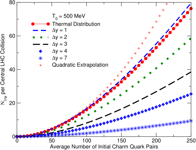
Figure 35: The $J/\psi$ production per central LHC collision in the kinetic model as a function of the initial number of $c\overline{c}$ pairs.

The corresponding centrality dependence is presented in Fig. 36, where we give $N_{J/\psi}$ at hadronization for three different initial charm quark momentum distributions, thermal, $\Delta y=4$ and $\Delta y=7$, as well as for our three choices of $N_{c\overline{c}}(b=0)$.

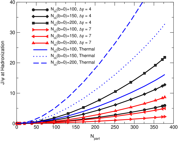
Figure 36: The centrality dependence of $J/\psi$ production in the kinetic model.

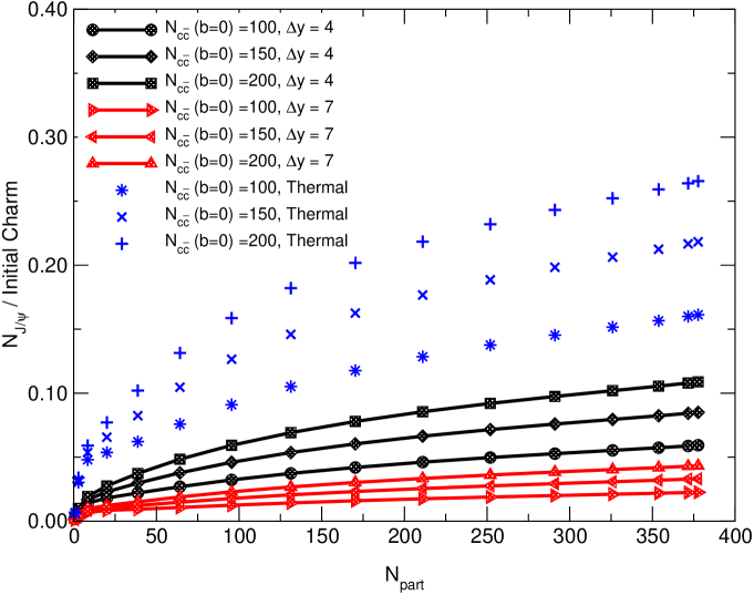
Figure 37: The ratio of the number of produced $J/\psi$’s in the kinetic model to the initial number of $c\overline{c}$ pairs as a function of $N_{\rm part}$.

Finally, the ratio of final $J/\psi$ to initial charm production is shown in Fig. 37 using the same parameters as in Fig. 35. These ratios are most easily compared to either initial production or suppression. There is a substantial variation in the predictions and it is evident that a simultaneous measurement of open charm will be required for an interpretation. However, the centrality dependence is opposite to that expected in any pure suppression scenario.

Table 17: Comparison of $J/\psi$ production at the LHC by the statistical hadronization (left-hand side) and kinetic formation (right-hand side) models.

	$dN_{J/\psi}/dy$ (Statistical)			$N_{J/\psi}$ (Kinetic, LO Charm)
	$dN_{c\overline{c}}(0)/dy$			$N_{c\overline{c}}(0)$
$b$ (fm)	25	18.75	12.5	200	150	100
0	0.656	0.370	0.165	4.0	2.26	1.03
1	0.637	0.359	0.160	3.85	2.19	1.00
2	0.586	0.330	0.147	3.51	2.00	0.91
3	0.515	0.290	0.130	3.04	1.73	0.79
4	0.434	0.245	0.109	2.50	1.43	0.65
5	0.351	0.198	0.088	1.97	1.12	0.51
6	0.270	0.152	0.068	1.46	0.84	0.38
7	0.196	0.110	0.050	1.01	0.58	0.27
8	0.132	0.075	0.034	0.65	0.38	0.18
9	0.082	0.046	0.021	0.38	0.22	0.10
10	0.045	0.026	0.012	0.20	0.12	0.057
11	0.022	0.013	0.0061	0.087	0.054	0.028
12	0.0097	0.0058	0.0029	0.034	0.022	0.012
13	0.0045	0.0029	0.0016	0.011	0.0075	0.0041
14	0.0028	0.0019	0.0012	0.0021	0.0013	$6.8\times 10^{-4}$
15	0.0025	0.0018	0.0012	$1.8\times 10^{-4}$	$1.0\times 10^{-4}$	$5.1\times 10^{-5}$

We have updated the calculations to include the charm quark momentum distribution from a leading order pQCD calculation [178]. The rapidity distribution has a somewhat larger effective $\Delta y$ and the $p_{T}$ distribution does not fall as fast as a simple Gaussian. As a result, the formation efficiency is further reduced. Such distributions may be most relevant, given preliminary results from RHIC [179, 180].

Table 18: Kinetic $J/\psi$ formation at the LHC assuming both thermal charm momentum (left-hand side) and $\Delta y=4$ (right-hand side).

	$N_{J/\psi}$ (Thermal)			$N_{J/\psi}$ ($\Delta y=4$)
	$N_{c\overline{c}}(0)$			$N_{c\overline{c}}(0)$
$b$ (fm)	200	150	100	200	150	100
0	52.7	32.5	16.4	17.5	10.8	5.48
1	50.5	31.2	15.8	16.8	10.4	5.25
2	44.8	27.7	14.0	14.9	9.21	4.65
3	37.0	22.9	11.5	12.3	7.62	3.82
4	28.6	17.7	8.73	9.54	5.89	2.90
5	20.7	12.7	6.05	6.90	4.23	2.01
6	13.8	8.32	3.72	4.61	2.77	1.24
7	8.28	4.71	2.14	2.76	1.57	0.71
8	4.10	2.36	1.10	1.36	0.79	0.37
9	1.78	1.04	0.50	0.59	0.35	0.16
10	0.65	0.39	0.19	0.22	0.13	0.064
11	0.19	0.12	0.063	0.065	0.040	0.021
12	0.048	0.032	0.018	0.016	0.010	0.006
13	0.011	0.0078	0.0049	0.0037	0.0026	0.0016
14	0.0026	0.0019	0.0012	$8.6\times 10^{-4}$	$6.3\times 10^{-4}$	$4.1\times 10^{-4}$
15	$5.9\times 10^{-4}$	$4.4\times 10^{-4}$	$2.9\times 10^{-4}$	$2.0\times 10^{-4}$	$1.5\times 10^{-4}$	$9.7\times 10^{-5}$

The numerical values for $N_{J/\psi}$ are compared with the statistical hadronization model results for $dN_{J/\psi}/dy$ in Table 17. The overall magnitudes are comparable, although the centrality dependences differ somewhat. Thus details such as the resulting $J/\psi$ momentum distributions will be required to differentiate between these two models [178]. For completeness, $N_{J/\psi}$ for the thermal distributions and the assumption $\Delta y=4$ are presented in Table 18.

5.4 Conclusions

The ”smoking gun” signature of the quarkonium formation mechanism is the quadratic dependence on the total number of charm quarks. For central collisions at the LHC one expects that this feature will lead to a total $J/\psi$ rate greater than that produced by an incoherent superposition of the initial nucleon-nucleon collisions, even including suppression due to deconfinement effects. In addition, the centrality dependence can be used to identify the quadratic dependence on charm assuming that the initial charm production scales with the number of binary collisions. Binary scaling leads to an increase of the ratio of $J/\psi$ to initial charm as the collision centrality increases, independent of specific parameters which control the overall magnitudes. A simultaneous measurement of total charm will be essential for such conclusions to be drawn.

Uncertainties in the absolute magnitude of the formation process are inherent in the model parameters. For statistical hadronization, one can constrain the thermal parameters to within a factor of two using the observed hadron populations. There is some additional uncertainty related to the lower cutoff on centrality needed to ensure the quarkonium ratios are consistent with an overall thermal picture. There is also the possibility that the correction for canonical ensemble effects will involve a thermal volume parameter not necessarily equal to the total system volume [181]. In addition, the formation mechanism could be limited to those charm quarks whose phase space separation is within some maximum value, introducing another as yet unconstrained parameter [170]. With kinetic formation, a similar set of uncertainties exist. There are uncertainties in the space-time properties of the deconfinement region. In addition, possible variations of charmonium binding energies and reaction cross sections in a deconfined region are at present not well understood. There are indications that the efficiency of the formation mechanism is considerably reduced when included in a partonic transport calculation [182].

The primary uncertainty in both models is still the initial number of charm quarks and their momentum distributions. The tabulated $J/\psi$ results should be regarded in this light. Thus numbers may be only an order of magnitude estimate. However, the variation with centrality and total initial charm should provide experimental signatures which are largely independent of the overall magnitudes.

Acknowledgments My thanks to Anton Andronic for discussions on the Statistical Model and Martin Schroedter for updates on the Kinetic Model calculations.

6 QUARKONIA IN HOT QCD MATTER: DISSOCIATION RATES 

6.1 Introduction

Quarkonium suppression was long ago suggested as a signal of deconfinement [1]. Due to their small size, quarkonia can, in principle, survive the deconfinement phase transition. However, because of color screening, no bound state can exist at temperatures $T>T_{D}$ when the screening radius, $1/\mu_{D}(T)$, becomes smaller than the typical bound-state size [1]. Later it was realized that dramatic changes in the gluon momentum distributions at the deconfinement phase transition result in a sharp increase in the quarkonium dissociation rates [175, 183, 184]. Both the magnitude [185] and the energy dependence [186] of charmonium dissociation by gluons result in a significant suppression of the $c\overline{c}$ states even for $T<T_{D}$ but higher than deconfinement transition temperature, $T_{c}$. Moreover, close to $T_{D}$ the thermal activation mechanism is expected to dominate [187, 188]. The relative importance of gluon dissociation and thermal activation is governed by the ratio of the quarkonium binding energy $\varepsilon(T)$ and the temperature $T$, $X(T)\equiv\varepsilon(T)/T$ [189]. At $X(T)\ll 1$ thermal activation dominates while for $X(T)\gg 1$ the dominant mechanism is “ionization” by gluons.

The study of quarkonium dissociation via color screening provides an upper bound on the temperature at which quarkonium bound states can exist. This temperature is also referred to as the Mott temperature [190]. We note, however, that resonances may still exist above the Mott temperature [191].

The dissociation temperature due to color screening was studied using potential models with different parameterizations of the heavy quark potential [27, 190, 192, 193]. All these studies predicted that excited charmonium states ($\chi_{c}$, $\psi^{\prime}$) will essentially dissolve at $T_{c}$ while the ground state $J/\psi$ will dissociate at $1.1~{}T_{c}$–$1.3~{}T_{c}$. Some potential models also predicted strong change in the binding energy, see e.g. Ref. [192]. Recently, charmonium properties were investigated using lattice calculations [194, 195] which indicate that the ground states exist with essentially unchanged properties at temperatures around $1.5T_{c}$. This issue will be discussed in section 6.2. Lattice investigations may indicate that at low temperatures, $T<1.5T_{c}$, screening is not efficient and therefore gluon dissociation may be the appropriate source of quarkonium suppression, discussed in section 6.3. Finally the equilibrium survival probabilities are estimated in section 6.4.

One should keep in mind that nonequilibrium effects in the very early stages of a heavy-ion collision, when the energy density is highest, should be also considered for quarkonium suppression. Not much is known about these effects. However, they may be an even more important source of quarkonium suppression than those of the thermalized system, see e.g. Ref. [196].

6.2 Investigation of In-medium Quarkonium Properties on the Lattice

Temporal meson correlators $\Delta(\tau,\vec{p})$ may allow direct study of in-medium quarkonium properties since they are related to the $T\neq 0$ spectral functions $\sigma(\omega,\vec{p},T)$ by

$$\Delta(\tau,\vec{p})=\int_{0}^{\infty}d\omega\,\sigma(\omega,\vec{p},T)\frac{\cosh(\omega(\tau-1/(2T)))}{\sinh(\omega/(2T))}.$$ (68)

Because at finite temperature, $T\neq 0$, the extension of the time direction is limited by the inverse temperature, the only way to study meson properties is to reconstruct the spectral function. The reconstruction of the spectral function with any reasonable discretization of the $\omega$ -interval involves reconstruction of several hundred degrees of freedom from $N_{\tau}\sim 10$ data points on $\Delta(\tau,\vec{p})$ where $N_{\tau}$ is the number of time-slices. In general, this can be done only using the so-called Maximum Entropy Method (MEM) [197, 198]. For a review see Ref. [198] and references therein. The method has also been quite successful at finite temperature [199, 200].

If we consider point sources, the correlators are defined as

$$\Delta(\tau,\vec{p})=\langle O(\tau,\vec{p})O(0,\vec{p})\rangle,$$ (69)

where

$$O(\tau,\vec{p})=\sum_{\vec{x}}e^{i\vec{p}\vec{x}}\overline{q}(\tau,\vec{x})\Gamma q(\tau,\vec{x}),$$ (70)

and $\Gamma=1$, $\gamma_{5}$, $\gamma_{\mu}$ and $\gamma_{\mu}\gamma_{5}$ for the scalar, pseudo-scalar, vector and axial-vector channels. By checking the quantum numbers one realizes that the ${}^{1}S_{0}$, ${}^{3}S_{1}$, ${}^{3}P_{0}$ and ${}^{3}P_{1}$ states actually correspond to the pseudo-scalar, vector, scalar and axial-vector channels.

One can also consider correlators of extended operators (sources)

$$O^{\rm ext}(\tau,\vec{p})=\sum_{\vec{x}}e^{i\vec{p}\vec{x}}\sum_{\vec{y}}\phi(\vec{y})\overline{q}(\tau,\vec{x}+\vec{y})\Gamma q(\tau,\vec{x}),$$ (71)

where $\phi(\vec{y})$ is some trial quarkonium wave function which typically has the form $\exp(-ay^{p})$ [194, 201]. Extended operators have a better overlap with the ground state than a point source. Though the spectral functions of extended operators are easier to reconstruct due to their simplified structure, typically a single pole, they have the disadvantage of introducing a bias by the choice of some specific trial wavefunction. They also do not correspond to any physically observable quantity such as the dilepton rate. The only information the study of such correlators can provide is the position and width of the resonance, provided that the corresponding structure of the spectral function can be interpreted as a narrow resonance.

The following discussion is primarily based on the finite temperature charmonium analysis of Ref. [195]. In this study, the nonperturbative clover action for quarks [202] was used with isotropic lattices, those with the same spacing in the temporal and spatial directions, with inverse lattice spacing, $a^{-1}$, between $4.04$ GeV and $9.72$ GeV. The quark mass was varied in a range corresponding to the pseudo-scalar $\eta_{c}(^{1}S_{0})$ mass between $2.4$ GeV and $4.1$ GeV.

Table 19: The lattice parameters used in the studies where $g^{2}$ is the lattice coupling, $T_{c}$ is the critical temperature for deconfinement. The lattice spacing $a$ is obtained from the string tension. The hopping parameter $\kappa$ is related to the quark mass by $m_{q}a=(1/2\kappa-1/2\kappa_{c})/u_{0}$ where $u_{0}$ is the average value of the link field and $\kappa_{c}(g^{2})$ was calculated in Ref. [202].

$6/g^{2}$	$a^{-1}$ (GeV)	Size	$T/T_{c}$	$\kappa$
6.499	4.042	$48^{3}\times 16$	0.93	0.1300, 0.1234
6.499	4.042	$48^{3}\times 12$	1.25	0.1300, 0.1234
6.499	4.042	$48^{3}\times 10$	1.5	0.1300, 0.1234
6.640	4.860	$48^{3}\times 16$	1.1	0.1290
6.640	4.860	$48^{3}\times 12$	1.5	0.1290
7.192	9.720	$64^{3}\times 24$	1.5	0.13114
7.192	9.720	$48^{3}\times 12$	3.0	0.13114

The parameters of the simulations are summarized in Table 19. The results of this study are compared to another study [194] using a standard Wilson action for quarks with anisotropic lattices and extended operators. The temporal lattice spacing in this study was four times smaller than the spatial one, $1/(2.03\,{\rm GeV})$, allowing more points in the time direction while keeping the spatial volume reasonably large. On the other hand, the large spacing in the spatial direction may result in many unwanted lattice artifacts. Both studies were done in the quenched approximation, neglecting the effects of quark loops. This approximation was used because such studies need quite small lattice spacings both because of the heavy quark mass and the need to have many points in the time direction, $N_{\tau}$, while keeping the temperature $1/(aN_{\tau})=T$ fixed. Going beyond this approximation would require more than 10 Teraflops of computational power.

The temperature dependence of the temporal correlators alone can provide some information on the change of the meson spectral properties. In Fig. 38 we show the ratio of the correlators at different temperatures to the free correlators calculated on the lattice for quark masses corresponding to a ${}^{1}S_{0}$ mass of $2.4$ GeV. As seen in the figure, the correlators in the pseudo-scalar and vector channels show only a very small temperature dependence across $T_{c}$ while in the scalar and axial-vector channels there are quite noticeable changes. This difference may imply that the ground state charmonia are not affected by deconfinement while the excited $1P$ states are.

  

Figure 38: The temporal correlators for different channels at $6/g^{2}=6.499$ and $\kappa=0.13$. The left-hand side shows the pseudo-scalar and vector channels, the right-hand side, the scalar and axial-vector channels.

This conclusion seems to be supported by the analysis of the spectral functions shown in Fig. 39. While the spectral function in the pseudo-scalar channel peaks at almost the same position at $0.93T_{c}$ and $1.25T_{c}$, in the axial-vector channel the peak present below $T_{c}$ is completely absent above $T_{c}$. The same results apply to the vector and scalar channels. Thus it seems that $1S$ ground state quarkonia are present above $T_{c}$ with essentially unchanged masses but the excited $1P$ states disappear already at $T\sim 1.25T_{c}$. The behavior of the correlators in Fig. 38 suggests that situation is similar at $1.5T_{c}$. To see what actually happens at temperatures of $1.5T_{c}$ or higher one has to consider simulations with lattice spacings $a^{-1}=4.86$ GeV and $a^{-1}=9.72$ GeV with $N_{\tau}\geq 12$. The analysis of the spectral functions in the pseudo-scalar and vector channels calculated with $a^{-1}=4.86$ GeV shows that the ground state peak survives at least until $1.5T_{c}$ and the spectral functions are essentially unchanged for $1.1T_{c}\leq T\leq 1.5T_{c}$ while the scalar and axial-vector spectral functions are similar to those at $1.5T_{c}$. This conclusion is also supported by the analysis of the spectral functions at $1.5T_{c}$ with $a^{-1}=9.72$ GeV. However, at $3T_{c}$ the spectral functions do not show any peak-like structures. On the other hand, the correlators show quite sizable changes between $1.5T_{c}$ and $3T_{c}$.

Finally we discuss the results obtained using extended operators [194]. Here only the pseudo-scalar and vector channels were considered. The simulations were done at two temperatures, $T=0.88T_{c}$ and $1.08T_{c}$. The spectral functions were first extracted using the MEM. Due to use of extended sources, the spectral functions essentially consist of a single peak with a temperature-independent position. Thus the authors of Ref. [194] used a $\chi^{2}$ fit to a Breit-Wigner function to determine

  

Figure 39: The spectral function for the pseudo-scalar (right) and axial-vector (left) channels at $0.93T_{c}$ and $1.25T_{c}$ and for $6/g^{2}=6.499$ and $\kappa=0.1300$.

the thermal width $\Gamma(T)$, obtaining

$${}^{1}S_{0}:\Gamma(T=1.08\,T_{c}) = 0.12\pm 0.03\,{\rm GeV},$$

$${}^{3}S_{1}:\Gamma(T=1.08\,T_{c}) = 0.21\pm 0.03\,{\rm GeV}.$$

The picture which emerges from the results of the lattice studies described above can be summarized as follows. The ground state quarkonia survive up to $\sim 1.5T_{c}$. Moreover, its mass does not change significantly relative to its $T=0$ mass, contrary to potential model predictions which show significant mass shifts as well as dissociation of ground state charmonia well below $1.5T_{c}$ [27, 192]. Thus screening is not an efficient mechanism for charmonium dissociation at temperatures close to $T_{c}$. However, there are indications that the ground state charmonia acquire a thermal width, implying that collisions with gluons may be the dominant mechanism for quarkonium dissociation at low temperatures. As the temperature increases, screening becomes more and more important and will lead to the disappearance of any bound state. The present study only indicates that in the absence of dynamical fermions this dissociation will happen somewhere between $1.5T_{c}$ and $3T_{c}$. The excited $1P$ states seems to dissolve already at $\sim 1.25T_{c}$, probably because the $1P$ state is larger than the ground state and therefore screening may be sufficient to dissolve it.

We now discuss whether these results can be interpreted within the present understanding of finite temperature QCD. First we note that the detailed picture of screening depends on the quantity one considers. Universal screening can be understood in terms of a simple (perturbative) picture only at astronomically high temperatures due to additional infrared problems arising at finite temperature. For a review, see e.g. Ref. [203]. The most relevant quantity as far as the finite temperature properties of quarkonium are concerned is probably the color singlet free energy, $F_{1}(r,T)$, studied in Ref. [205]. This quantity shows quite complex short distance behavior and cannot be parameterized by any simple form. Nevertheless, for $T_{c}<T<1.5T_{c}$, a rough estimate of the screening length is $0.4-0.6$ fm. From the small value of the screening length, it is possible to conclude that the charmonium ground state should also dissolve below $1.5T_{c}$. However, the free energy also contains an entropy contribution, $S(r,T)=-\partial F_{1}(r,T)/\partial T$ and therefore is not directly related to the potential between static charges. In fact, at large distances the entropy is positive. Therefore the free energy, $F_{1}(r,T)=V_{1}(r,T)-TS(r,T)$, is always smaller than the potential energy $V_{1}(r,T)$ [205]. If this situation persists over all distances it would imply that screening in $F_{1}$ is stronger than in $V_{1}$, and could possibly explain the discrepancy between the lattice studies of the charmonium spectral functions and potential models.

6.3 Quarkonium Dissociation Cross Sections and Rate Coefficients

In this section, we evaluate the dissociation rates of Coulombic bound states by collisions in a quark-gluon plasma. For the first step, the plasma is represented by an ideal gluon gas with thermal distribution functions $n_{g}(\omega)=g_{g}[\exp(\omega_{g}(p)/T)-1]^{-1}$, where $T$ is the temperature, $\omega_{g}(p)$ is the dispersion relation and $g_{g}=2(N_{c}^{2}-1)$ is the gluon degeneracy factor with $N_{c}=3$. We focus here on the ${}^{3}S_{1}$ quarkonium ground states, $J/\psi$ and $\Upsilon$, which we consider to be Coulombic bound states. Their masses are expected to be rather independent of the plasma temperature, as discussed in section 6.2. These results are consistent with experimental results for excitonic states in an electron-hole plasma [191] and with dynamical screening [190] as opposed to static Debye screening [193]. The effects of lowering the continuum threshold as well as temperature dependent modifications of the heavy quark potential will be neglected in this first step.

The quarkonium breakup cross section by gluon impact can be estimated using the Bhanot–Peskin formula [186],

$$\sigma_{(Q\overline{Q})g}(\omega)=\frac{2^{11}}{3^{4}}\alpha_{s}\pi a_{0}^{2}\frac{(\omega/\varepsilon(0)-1)^{3/2}}{(\omega/\varepsilon(0))^{5}}\Theta(\omega-\varepsilon(0))\,\,,$$ (72)

where $\varepsilon(0)$ is the $T=0$ binding energy of the $1S$ quarkonium state with a Coulombic rms radius $\sqrt{\langle r^{2}\rangle_{1S}}=\sqrt{3}a_{0}=2\sqrt{3}/(\alpha_{s}m_{Q})$, $m_{Q}$ is the heavy-quark mass and $\omega$ is the energy of the incoming gluon. The values of $m_{Q}$ and $\varepsilon(0)$ used in our further calculations are given in Table 20.

Table 20: Values of binding energy, $\varepsilon(0)$, and heavy quark mass, $m_{Q}$, [206] used in our further calculations.

	Set (i)		Set (ii)
System	$\varepsilon(0)$ (GeV)	$m_{Q}$ (GeV)	$\varepsilon(0)$ (GeV)	$m_{Q}$ (GeV)
bottomonium	0.75	5.10	1.10	5.28
charmonium	0.78	1.94	0.62	1.86

The Bhanot–Peskin formula is derived using the operator product expansion, keeping the leading color–electric dipole operators to leading order in $1/N_{c}$, so that the final-state colour octet interactions of heavy-quark pair are negligible. The corresponding expression for the Wilson coefficients (chromo–electric polarizabilities) of the excited $1P$ states is given in Ref. [207]. Since quarks have been found to be less efficient in dissociating quarkonium states [183], we only include the effects of gluons here.

The cross section in Eq. (72) has a steep rise at threshold with a drop after the maximum. We give the thermal–averaged cross sections in Fig. 40.

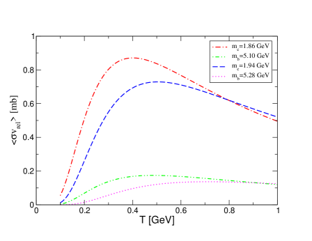
Figure 40: Thermal averaged cross sections for heavy quarkonium dissociation by gluon impact as a function of temperature.

A straightforward extension to the $p_{T}$ dependence of the quarkonium state in the plasma has been studied in Ref. [184].

The dissociation rate for a quarkonium $1S$ state at rest in a heat bath of massless gluons at temperature $T$ distributed according to $n_{g}(\omega)$ is

$$\tau_{(Q\overline{Q})g}^{-1}(T)\equiv\Gamma_{(Q\overline{Q})g}(T)=\langle\sigma_{(Q\overline{Q})g}(\omega)n_{g}(\omega)\rangle_{T}~{}.$$ (73)

Results for the partial widths $\Gamma_{(Q\overline{Q})g}$ due to collisions, together with their inverses corresponding to partial lifetimes, are shown in Fig. 41 for gluon breakup. It is interesting to note that there is close correspondence between the charmonium decay widths due to gluon impact, the gluonic E1 transition, and the widths extracted from recent lattice simulations in the previous section.

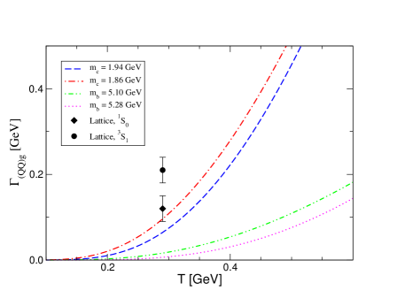
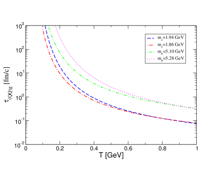
Figure 41: The rate coefficients $\Gamma_{(Q\overline{Q})g}=\tau_{(Q\overline{Q})g}^{-1}$ for heavy quarkonium dissociation by gluon impact as a function of the gluon plasma temperature (left panel) and the corresponding lifetime $\tau_{(Q\overline{Q})g}$ (right panel). For comparison, the Breit-Wigner fits to the ${}^{1}S_{0}$ and ${}^{3}S_{1}$ charmonium spectral widths from lattice simulations are shown.

6.4 Quarkonia Abundancies and Observable Signatures

In order to study observable signatures, we adopt the Bjorken scenario [208] of plasma evolution, i.e. a longitudinal expansion with conserved entropy: $T^{3}\tau=T_{0}^{3}\tau_{0}={\rm const}$. The initial temperatures and proper times are give in Table 21. The RHIC and LHC values are set 3 from Ref. [184], assuming the highest initial fugacities. The SPS values are typical of those used in Ref. [208].

Table 21: Initial conditions for plasma evolution. The results for LHC and RHIC are from Ref. [184].

	LHC	RHIC	SPS
$T_{0}$ [GeV]	0.72	0.4	0.25
$\tau_{0}$ [fm/$c$]	0.5	0.7	1.0

We calculate the quarkonium survival probability neglecting nucleon absorption, hadronic comovers and hadronization effects,

$$S(\tau_{f})=\exp\left(-\int_{\tau_{0}}^{\tau_{f}}~{}d\tau~{}\tau_{(Q\overline{Q})g}^{-1}(T)\right)~{}.$$ (74)

At the freeze-out time, $\tau_{f}$, the collisions stop changing the number of $J/\psi$ and $\Upsilon$. Using Bjorken scaling, $\tau_{f}$ can be translated into a freeze-out temperature. In Fig. 42 we show the survival probability of $J/\psi$ (left panel) and $\Upsilon$ (right panel) due to gluon impact using the initial conditions from Table 21. Note that set (i) gives the lowest $\Upsilon$ survival probability due to its lower values of the binding energy and bottom quark mass while set (ii), with its lower charmonium binding energy and charm mass, has the lower survival probability for the $J/\psi$.

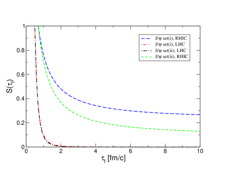
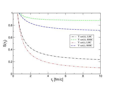
Figure 42: The survival probabilities of heavy quarkonia in a longitudinally expanding gluon plasma as a function of the plasma lifetime using the initial conditions of Table 21 and the heavy quark masses and binding energies of Table 20. On the left-hand side are the $J/\psi$ results and on the right-hand side are the $\Upsilon$ results.

The simple estimates presented here for the LHC suggest that none of the initially produced $J/\psi$’s will survive their passage through the plasma. An analysis of the $p_{T}$ dependence of the suppression pattern, as in Ref. [184], should provide a more complete picture. The $\Upsilon$, however, will be a good probe of the plasma lifetime as well as its temperature.

6.5 Conclusions

We have used recent lattice data on the mesonic spectral functions to constrain predictions of the temperature dependence of the two-particle quarkonium spectra. We have evaluated the collisional broadening of quarkonia states in a quark-gluon plasma using the Bhanot-Peskin cross section. The $J/\psi$ partial widths in a gluon gas are in good agreement with lattice results for the spectral widths without dynamical fermions.

Neglecting secondary quarkonium production we have evaluated the time dependence of the survival probability of $J/\psi$ and $\Upsilon$ for different initial conditions. The results suggest that measurements of $\Upsilon$ suppression at the LHC can provide rather robust information about the initial temperature or lifetime of the QGP [209].

Acknowledgments D.B. would like to thank Yuri Kalinovsky and Gerhard Burau for useful discussions.

7 HEAVY QUARK PRODUCTION IN MONTE CARLO GENERATORS 

7.1 Introduction

This section presents a study of the predictions of Monte Carlo parton shower programs for the generation of charm and bottom quarks in heavy-ion collisions at LHC energies. In section 7.2 the production cross sections in nucleon-nucleon collisions, calculated at the next-to-leading order (NLO), and their extrapolations to Pb+Pb collisions are reported. The NLO kinematical distributions are then compared with the results obtained with pythia [210, 211] and herwig [212, 213, 214] in sect. 7.3 and sect. 7.4 respectively. Section 7.5 presents a short description of hijing [215, 216], a generator for nucleus-nucleus collisions, used to simulate the charm- and bottom-hadron production background in $AA$ collisions.

7.2 NLO heavy flavour production cross sections at the LHC

The cross sections for charm and bottom production in $pp$ collisions at LHC energies, $\sqrt{s}=5.5\ \mathrm{TeV}$ and 14 TeV, have been calculated at NLO using a program by Mangano, Nason and Ridolfi [5] (referred to as MNR hereafter). Two sets of parton distribution functions, MRST [24] and CTEQ5M1 [25], have been used. All the following MNR calculations have been performed using the same values for the heavy quark masses ($m_{c}$ and $m_{b}$) and the factorization and renormalization scales ($\mu_{F}$ and $\mu_{R}$) as in Ref. [177]:

$$m_{c} = 1.2\,\,\mathrm{GeV}\,,\,\,\,\,\,\,\,\,\,\,\,\,\,\,\,\,\,\,\,\,\,\,\,\,\,\,\,\,\,\,\,\,\,\,\,\,\,\,\,\mu_{F}=\mu_{R}=2\,\mu_{0}\,,$$ (75)

$$m_{b} = 4.75\,\,\mathrm{GeV}\,,\,\,\,\,\,\,\,\,\,\,\,\,\,\,\,\,\,\,\,\,\,\,\,\,\,\,\,\,\,\,\,\,\,\,\,\,\,\,\,\mu_{F}=\mu_{R}=\mu_{0}\,,$$ (76)

where $\mu_{0}=m_{Q}$ in calculations of the total cross section and $\mu_{0}=\sqrt{(p_{T,Q}^{2}+p_{T,\overline{Q}}^{2})/2+m_{Q}^{2}}$ for differential cross sections. The $pp$ results are reported in Table 22. The difference due to the choice of the parton distribution functions is relatively small, $\sim 20-25$% at 5.5 TeV and slightly less at 14 TeV. In $AA$ collisions, the cross section per nucleon is modified by shadowing which we implement using the EKS98 parameterization [16, 17].

A discussion of the inclusive heavy quark $p_{T}$ and $y$ spectra and the $Q\overline{Q}$ correlations is presented in the following section. The NLO predictions are also compared to results obtained using pythia.

Table 22: NLO calculation [5] of the total $c\overline{c}$ and $b\overline{b}$ cross sections in $pp$ collisions at 5.5 and 14 TeV, using the MRST and CTEQ5M1 parton distribution functions.

		$\sigma_{pp}$ (mb)
$\sqrt{s}$ (TeV)	$Q\overline{Q}$	MRST	CTEQ5M1
	$c\overline{c}$	5.86	7.42
5.5	$b\overline{b}$	0.19	0.22
	$c\overline{c}$	10.28	12.07
14	$b\overline{b}$	0.46	0.55

7.3 Heavy flavour production in pythia

The MNR code is not well suited for simulation purposes since it is not an event generator. Also, at LHC energies the NLO corrections are large. Therefore still higher order corrections may be important because of, e.g., multiple gluon emission. On the other hand, Monte Carlo event generators like pythia and herwig offer a different set of approximations. They are based on LO pQCD matrix elements and parton showers which simulate real corrections to LO QCD processes. For example, a final state heavy quark can further radiate a gluon or an initial-state gluon can split into a quark-antiquark pair. The parton shower approach to contributions beyond LO is not exact even at NLO but it catches the leading-log aspects of multiple-parton emission.

In the simulations described here, pythia 6.150 was used. We will indicate light quarks ($u$, $d$ or $s$) by $q$ and charm or bottom quarks by $Q$.

7.3.1 Comparison with LO MNR results

On general grounds, one expects that the LO description of $Q\overline{Q}$ production should be the same in pythia and MNR when parton showers are turned off in pythia. Thus before comparing the results of the full pythia simulation with the ones obtained with the NLO MNR calculation, we first check if the basic LO subprocesses are handled correctly in pythia. We compare the pythia calculations without initial and final-state showers to the MNR LO results in $\sqrt{s}=5.5$ TeV $pp$ collisions for the following observables:

• inclusive $p_{T}$ and rapidity distribution of the $Q$ ($\overline{Q}$);

• pair $p_{T}$, defined as the projection on the plane normal to the beam axis of the $Q\overline{Q}$ total momentum $\mathbf{p}_{Q}+\mathbf{p}_{\overline{Q}}$;

• pair mass, $M(Q\overline{Q})=\sqrt{(E_{Q}+E_{\overline{Q}})^{2}-(\mathbf{p}_{Q}+\mathbf{p}_{\overline{Q}})^{2}}$, where $E_{Q}=\sqrt{m_{Q}^{2}+(\mathbf{p}_{Q})^{2}}$ is the quark energy;

• angle $\Delta\phi$ between the $Q$ and the $\overline{Q}$ in the plane normal to the beam axis.

The results for charm production via gluon fusion, $gg\rightarrow c\overline{c}$, are shown in Fig. 43. For a meaningful comparison the same input parameters were used in pythia and in MNR. We use the CTEQ4L parton densities with a two-loop evaluation of $\alpha_{s}$, $m_{c}=1.2$ GeV, $\mu_{F}=\mu_{R}=\mu=2\sqrt{(p_{T}^{\rm hard})^{2}+m_{c}^{2}}$ where $p_{T}^{\rm hard}$ is the quark transverse momentum in the lab frame. Parton intrinsic momentum smearing is modeled by a Gaussian with $\langle k_{T}^{2}\rangle=1$ GeV².

Figure 43: Comparison between pythia results (solid histogram) for $gg\rightarrow c\overline{c}$, without parton showers, and the MNR calculation of the same process at LO (dashed histogram). The centre of mass energy is $\sqrt{s}=5.5\ \mathrm{TeV}$.

Multiple interactions and initial and final-state parton showers were switched off in pythia for this comparison.

The level of agreement between the two calculations is excellent. Thus the LO calculations in both methods gives the same results when the same parameters are used. Since at LO the pair is produced back-to-back, the $p_{T}$ of the pair should be zero and $\Delta\phi=\pi$. The deviation from the strict back-to-back configuration is due to the intrinsic $k_{T}$ of the incoming partons. The $k_{T}$-kick is implemented differently in the two calculations. Thus the fact that MNR and pythia give the same results for this value of $\langle k_{T}^{2}\rangle$ is quite remarkable. However, this fact should be considered as accidental, and one should not expect it to hold in general, for example for larger values of $\langle k_{T}^{2}\rangle$.

7.3.2 Parton shower and process classification in pythia

When the parton shower is included, the partonic interaction can be subdivided in different stages. The event generation starts with the LO process and then the parton shower is used to generate different histories for the incoming and outgoing particles that take part in the LO process. For example, outgoing particles from the LO process can emit gluons or an incoming charm quark could come from the splitting of a gluon into a $Q\overline{Q}$ pair. Therefore the parton shower will shift the kinematics of the produced particles and at the same time can increase the multiplicity of final state. The parton showers do not affect the probabilities of the LO processes but increase the total rate of heavy quark production through gluon splitting into $Q\overline{Q}$ pairs.

In pythia the processes are divided in the following three classes, according to the number of heavy quarks in the final state of the hard process, where the hard process is defined as the one with the highest virtuality:

pair creation:

The hard process produces two heavy quarks in the final state through the reactions $gg\rightarrow Q\overline{Q}$ and $q\overline{q}\rightarrow Q\overline{Q}$; these are the reactions which constitute the LO contribution in MNR;

flavour excitation:

A heavy quark in one incoming hadron is put on mass shell by scattering off a parton from the opposite hadron, $qQ\rightarrow qQ$ or $gQ\rightarrow gQ$. The incoming heavy quark is assumed to come from a $g\rightarrow Q\overline{Q}$ splitting in the initial-state shower. This hard process is characterized by one heavy quark in the final state;

gluon splitting:

No heavy quark is involved in the hard scattering. Instead a $Q\overline{Q}$ pair is produced in the initial or final-state showers from a $g\rightarrow Q\overline{Q}$ branching.

This classification might be misleading since all three classes produce pairs at $g\rightarrow Q\overline{Q}$ vertices when showers are turned on. However, the requirement that the hard scattering should be more virtual than the shower avoids double-counting [217]. Fig. 44 shows some topologies belonging to the processes specified above.

Figure 44: Examples of pair creation, flavour excitation and gluon splitting. The thick lines correspond to the hard process, the thin ones to the parton shower.

Flavour excitation and gluon splitting contributions are calculated in the approximation of massless quarks. As a consequence, these cross sections diverge as $p_{T}^{\rm hard}$ vanishes. These divergences are usually regularized by putting a lower bound on the allowed values of $p_{T}^{\rm hard}$. However, the choice of the minimum $p_{T}^{\rm hard}$ is arbitrary and is usually considered to be a parameter. The lower bound on $p_{T}^{\rm hard}$ has a strong influence on the heavy flavour cross section at low $p_{T}$. Experiments with acceptances starting at several GeV, such as CDF and DØ  at the Tevatron and ATLAS and CMS at the LHC, are not very sensitive to $p_{T}^{\rm hard}$. On the other hand, ALICE has been designed for good acceptance down to very low $p_{T}$ since the measurement of the total heavy flavour cross section in nuclear reactions is of great interest. Therefore, the choice of the minimum $p_{T}^{\rm hard}$ in the simulations of heavy quark production has to be carefully evaluated. The criteria used in this choice are explained in the next section.

7.3.3 Comparison with MNR at NLO and tuning of pythia parameters

Because of the divergence at low $p_{T}$, pythia does not offer a valid baseline for the calculation of the total cross section and of the kinematical distributions in the low-$p_{T}$ region. For this reason our approach has been to adopt the NLO calculation as the baseline for our simulations and to tune the pythia parameters to reproduce the NLO predictions as closely as possible. The main parameter tuned is the lower bound of $p_{T}^{\rm hard}$. The simulations of Pb+Pb collisions at $\sqrt{s}=5.5$ TeV/nucleon includes shadowing using the EKS parameterization [16, 17], as noted in section 7.2. The complete list of parameters used is shown in Table 23. See Ref. [210, 211] for a description of the pythia parameters. The larger value of the intrinsic $k_{T}$-kick in Pb+Pb relative to $pp$ collisions ($k_{T}$ broadening) has been taken from Ref. [177], based on a $Q^{2}$-dependent nuclear broadening.

Table 23: pythia parameters used for the generation of charm and bottom quarks for Pb+Pb collisions at $\sqrt{s}=5.5$ TeV/nucleon and $pp$ collisions at $\sqrt{s}=14$ TeV. All unspecified parameters are pythia 6.150 defaults.

description	parameter	Charm	Bottom
Process types	MSEL	1	1
Quark mass	PMAS(4/5,1)	1.2	4.75
Minimum $p_{T}^{\rm hard}$	CKIN(3)	2.1	2.75
CTEQ4L	MSTP(51)	4032	4032
Proton PDF	MSTP(52)	2	2
Switch off	MSTP(81)	0	0
multiple	PARP(81)	0	0
interactions	PARP(82)	0	0
Initial/Final parton	MSTP(61)	1	1
shower on	MSTP(71)	1	1
2nd order $\alpha_{s}$	MSTP(2)	2	2
QCD scales	MSTP(32)	2	2
for hard scattering	PARP(34)	1	1
and parton shower	PARP(67)	1	1
	PARP(71)	4	1
	MSTP(91)	1	1
	PARP(91)	1.304 (Pb+Pb)	2.035 (Pb+Pb)
Intrinsic $k_{T}$		1 ($pp$)	1 ($pp$)
	PARP(93)	6.52 (Pb+Pb)	10.17 (Pb+Pb)
		5 ($pp$)	5 ($pp$)

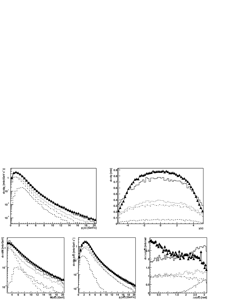
Figure 45: Comparison between charm production in the NLO calculation by Mangano, Nason and Ridolfi and in pythia with parameters tuned as described in the text for Pb+Pb collisions at $\sqrt{s}=5.5$ TeV/nucleon. The triangles show the NLO calculation, the solid histogram corresponds to the pythia total production. The individual pythia contributions are pair production (dashed), flavour excitation (dotted) and gluon splitting (dot-dashed).

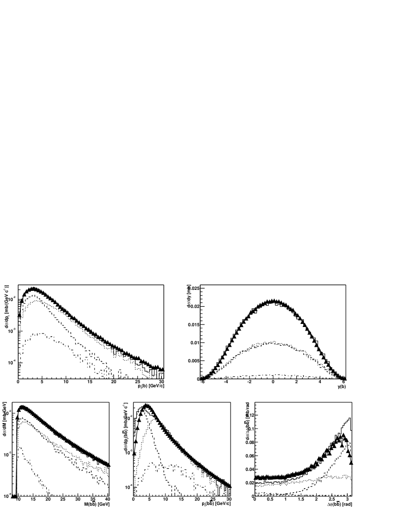
Figure 46: Same as Fig. 45, but for bottom production.

The results of this tuning for Pb+Pb collisions at 5.5 TeV/nucleon are shown in Fig. 45 for charm and in Fig. 46 for bottom. The pythia and NLO distributions are compared. The pythia results are scaled by factors of 0.62 and 0.57 respectively to give the same total cross section as the NLO calculation. Despite the fundamental differences between the two models, the agreement is relatively good. However, significant discrepancies are present, especially in the $\Delta\phi$ distribution of the charm quarks.

We note that the CTEQ4L parameterization used here is rather outdated. However, we verified with the MNR code, that these results lie in between those obtained with CTEQ5 and MRST for all the relevant kinematical quantities. The sensitivity to the parton distribution functions does not exceed 30% for charm and 20% for bottom. Figure 47 shows the inclusive $p_{T}$ and rapidity distributions for charm with the CTEQ4L, CTEQ5L and MRST distributions.

Figure 47: Inclusive $p_{T}$ and rapidity distributions for charm with the CTEQ4L, CTEQ5L and MRST structure functions. The distributions are obtained using the MNR code for Pb+Pb collisions at 5.5 TeV/nucleon.

Figure 48: Comparison between charm production in 14 TeV $pp$ interactions with the MNR code and pythia with parameters of Table 23. The curves are the same as those in Fig. 43 but now the MNR results are shown by the solid curves.

Figure 49: Same as Fig. 49, but for bottom production.

To simulate heavy quark production for the 14 TeV $pp$ run, the same parton distribution functions and values of $m_{Q}$ and $\mu$ are used, see Table 23. The comparison of the pythia spectra with the MNR calculation is shown in Fig. 49 for charm and in Fig. 49 for bottom. The largest difference is a rather poor description of the charm quark rapidity distribution due to the range of validity of the parton distribution functions. Most widely used parton distributions, including CTEQ4, are valid only down to $x\sim 10^{-5}$. Below this $x$, the behaviour depends on the implementation of the parton density but has no physical meaning. For example, the CTEQ4 gluon density is fixed to its value at $x=10^{-5}$. The rapidity range over which the evolution of the set of parton densities is reliable depends on the energy. For charm production at $\sqrt{s}=5.5$ and 14 TeV this range corresponds to $|y|<4.3$ and $|y|<3.4$ respectively.

7.3.4 Fragmentation and decay

We use the default pythia quark fragmentation and hadron decay parameters. Table 24 summarizes the total yield and the rapidity density, $dN/dy$, averaged over $|y|<1$ for heavy flavour hadrons.

Table 24: Total yield and average rapidity density for $|y|<1$ for hadrons with charm and bottom produced in Pb+Pb collisions at $\sqrt{s}=5.5$ TeV/nucleon.

Particle	Yield	$\langle dN/dy\rangle_{|y|<1}$	Particle	Yield	$\langle dN/dy\rangle_{|y|<1}$
$D^{0}$	68.9	6.87	$B^{0}$	1.86	0.273
$\overline{D}^{0}$	71.9	6.83	$\overline{B}^{0}$	1.79	0.262
$D^{+}$	22.4	2.12	$B^{+}$	1.82	0.251
$D^{-}$	22.2	2.00	$B^{-}$	1.83	0.270
$D_{s}^{+}$	14.1	1.30	$B_{s}^{0}$	0.53	0.077
$D_{s}^{-}$	12.7	1.22	$\overline{B}_{s}^{0}$	0.53	0.082
$\Lambda_{c}^{+}$	9.7	1.18	$\Lambda_{b}^{0}$	0.36	0.050
$\overline{\Lambda_{c}}^{-}$	8.2	0.85	$\overline{\Lambda_{b}}^{0}$	0.31	0.047

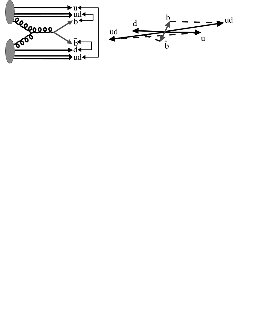
Figure 50: Sketch of the string structure for the LO graph $gg\rightarrow b\overline{b}$. Left: the heavy quark is attached to a beam remnant (quark or diquark). Right: the same view in momentum space (not to scale). The dashed lines represent strings.

The default fragmentation scheme in pythia is Lund string fragmentation. The string topology is derived from the colour flow in the hard process, determining the partonic partners in the colour singlet state forming the string endpoints. Let us consider, for example, one of the LO graphs contributing to $gg\rightarrow b\overline{b}$, see Fig. 50. The colour representation of the beam remnants is always described by a quark in a colour triplet state and a diquark in a colour anti-triplet state which thus behaves like an antiquark. Therefore, in this simple situation, there are only three strings, as shown in Fig. 50. The $b$ quark is colour connected to a diquark, the $\overline{b}$ is connected to a quark and the last string connects the remaining quark-diquark system. When we include the parton shower, the number of quarks in the final state increases and therefore more colour singlet strings can be produced. The strings then fragment according to the longitudinal Lund symmetric fragmentation function. For strings with heavy quark endpoints, the Lund fragmentation function is too soft to reproduce the charm and bottom meson fragmentation data. The Lund fragmentation function is therefore modified through the pythia default settings to take into account the harder spectrum of heavy flavour mesons using the Bowler parameterization. The fact that the heavy quark is usually connected with one of the beam remnants shifts the rapidity of the heavy quark towards the rapidity of the projectile or target [217], see Fig. 51.

Figure 51: Average difference between the rapidity of the B meson and the one of the corresponding b quark, as a function of the quark rapidity, for interactions with $p_{T}^{\rm hard}>m_{b}$.

A detailed description of the heavy quark string fragmentation can be found in Ref. [217]. Here we report only how it affects the kinematics. Figure 52 shows the charm $p_{T}$ and rapidity as well as the $p_{T}$ and $\Delta\phi$ distributions of the $c\overline{c}$ pairs. The solid histograms represent quarks and the dashed histograms, the charm mesons. In this figure we consider only the mesons into which the quarks hadronize. The decay of heavy flavor resonances is not included. Figure 53 shows the equivalent plots for bottom.

Figure 52: Distributions for charm quarks (solid histogram) and $D$ mesons (dashed histogram). The normalization is arbitrary.

Figure 53: Distributions for bottom quarks (solid histogram) and $B$ mesons (dashed histogram). The normalization is arbitrary.

The most important effect is a reduction of the transverse momenta, directly reflecting the magnitude of the longitudinal fragmentation function. The fragmentation reduces the momentum of charm mesons by 25% and of bottom mesons by 14% on average. The rapidity shift shown in Fig. 51 is much smaller than the rapidity range of the interactions. Therefore it does not strongly affect the inclusive rapidity distribution. The azimuthal correlation is also not significantly affected by fragmentation.

7.4 A study of heavy flavour production in herwig

Like pythia, herwig [212, 213, 214] is a general-purpose event generator which uses parton showers to simulate higher-order QCD effects. The main differences with respect to pythia are the treatment of the parton showers, which accounts more correctly for coherence effects, and the hadronization model, based on cluster rather than string fragmentation. The version used for the analysis presented here is herwig 6.4. Here we investigate the main features of heavy flavour production in herwig rather than trying to produce agreement between herwig and the NLO calculation. The following simulations have been done for $pp$ collisions at $\sqrt{s}=5.5$ TeV.

7.4.1 Comparison with LO MNR results

As with pythia, we first checked the description of the LO processes in herwig by comparing to the LO results of the MNR code. For the LO calculations, we used the same parameters in both calculations. We used the CTEQ4L parton distributions with $\Lambda_{\rm QCD}^{(4)}=236$ MeV, $m_{c}=1.2$ GeV, $m_{b}=4.75$ GeV and default herwig factorization and renormalization scales. Good agreement was found when the herwig parton showers were switched off.

7.4.2 Parton showers in herwig: gluon splitting and flavour excitation

Since gluon splitting and flavour excitation cannot be considered separately in the NLO code, as in event generators, we cannot compare the two results at this level. Instead we can compare herwig with pythia to see if there are fundamental differences in the implementation of these processes.

The gluon splitting results for bottom production are compared in Fig. 54. The shape of the distributions from the two generators agree at high $p_{T}$. Since different scales are used in herwig and pythia we do not expect the result to be exactly the same, especially at low $p_{T}$.

Figure 54: Gluon splitting results in $b\overline{b}$ production, obtained with herwig (solid) and pythia (dotted).

On the other hand, flavour excitation is clearly different in the two generators. The problem is apparent in the single quark $p_{T}$ spectrum where a large peak is present at $p_{T}\sim m_{b}$ when herwig is used. We studied the origin of this peak by comparing the single quark spectrum for the quark coming from the hard scattering and for the quark coming from the initial-state gluon splitting, the middle diagram in Fig. 44. We have performed this separation and we present the comparison in Fig. 55. We can see that, while the hard scattering part is compatible for the two models, herwig fails to describe the initial-state evolution of the gluon splitting into a $Q\overline{Q}$ pair. This may be due to the fact that initial-state shower variables in herwig are chosen for light parton showers and mass effects are not considered [218]. We found the same kind of behaviour for charm production although the peak in $p_{T}$ spectrum is shifted to a value closer to $m_{c}$. Given that herwig does not correctly describe flavour excitation in the low-$p_{T}$ region, it should not be used for simulations in such a region.

Figure 55: Comparison of flavour excitation in herwig and pythia. The distributions are divided into two parts, a heavy quark coming from hard scattering (hard) and from gluon splitting (branch), see Fig. 44.

7.5 hijing: event generator for nucleus-nucleus collisions

hijing (Heavy Ion Jet INteraction Generator) is widely used to simulate the background for feasibility studies of heavy flavour detection. hijing combines a QCD-inspired model of jet production [215, 216] with the Lund model for jet fragmentation. Hard or semi-hard parton scatterings with transverse momentum of a few GeV are expected to dominate high energy heavy ion collisions. The hijing model has been developed with special emphasis on the role of minijets in $pp$, $pA$ and $AA$ interactions at collider energies.

The Lund fritiof [219] model and the Dual Parton Model [220] have guided the formulation of hijing for soft nucleus-nucleus interactions at low energies, $\sqrt{s}\simeq 20$ GeV/nucleon. The hadronic collision model has been inspired by the successful implementation of perturbative QCD processes in pythia.

Two important features of nuclear collisions in hijing are the simulation of jet quenching and nuclear shadowing. The charged-particle rapidity-density given by hijing with jet quenching for central Pb+Pb collisions at $\sqrt{s}=5.5$ TeV/nucleon is $dN_{\rm ch}/dy\simeq 6200$, about a factor of 2 larger than that predicted using recent analyses of RHIC results [221]. However, such a large multiplicity can be considered as a “safety factor” for the feasibility studies. hijing also provides the relevant background sources such as direct leptons and strange particles.

7.6 Conclusions

We have studied heavy quark production in nucleon-nucleon collisions at LHC energies with the most widely used Monte Carlo generators—pythia and herwig. The resulting distributions were compared to those obtained in perturbative QCD to NLO using the MNR code [5] to establish a baseline simulation of heavy flavour production. We found that by tuning the main pythia parameters, satisfactory agreement with the NLO bare quark transverse momentum distributions was obtained for both charm and bottom production in $pp$ collisions at $\sqrt{s}=5.5$ and 14 TeV. The most important parameters tuned in the comparison were the heavy quark masses, the minimum $p_{T}^{\rm hard}$ of the heavy quarks in the lab frame, and the width of the transverse momentum smearing of the incoming partons, $\langle k_{T}^{2}\rangle$. However, we found that herwig does not treat flavour excitation correctly at small transverse momenta, making it unsuitable for simulations of heavy quark production.

This problem is solved by merging the NLO computations with parton showers, as advocated in MC@NLO [10, 222]. The implementation of heavy flavour hadroproduction, Ref. [10], became available after the completion of the work reported in this section. We point out that, in the context of MC@NLO, no additional tuning of the Monte Carlo parameters is needed to reproduce the NLO results in the relevant regions since this is guaranteed by the formalism.

8 QUARKONIA AND HEAVY FLAVOUR DETECTION WITH THE ALICE DETECTOR 

8.1 Introduction

ALICE is the dedicated heavy-ion experiment at the LHC. The apparatus will investigate strongly interacting matter at extreme energy densities by comprehensive measurements of a large variety of observables [223, 224]. Among the most promising observables, heavy flavours are especially relevant since they provide an essential probe of the earliest stage of heavy ion collisions. They further give precious information on the properties of the medium produced at longer time scales.

Quarkonium states can be pertinent signatures of the Quark Gluon Plasma (QGP). From the early predictions of charmonium suppression by Debye screening in a deconfined medium [1], to the recent results from the NA50 collaboration at SPS [225], much effort has been devoted to the subject (for reviews see Refs. [226, 227]). While at SPS energies only charmonium states are experimentally accessible, the much higher LHC (and RHIC) energies make bottomonium measurements feasible, thus providing an additional probe for QGP studies. In fact, since the $\Upsilon$(1S) state only dissolves significantly above the critical temperature [27, 188], at a value which might only be reachable at energies above that of RHIC, the spectroscopy of the $\Upsilon$ family at the LHC should reveal unique characteristics of the QGP [29]. We note also that quarkonium measurements at RHIC and LHC are complementary in terms of the accessible $x$ range.

The study of quarkonium states at the LHC is significantly different from those at the SPS and RHIC. First of all, in addition to prompt charmonia produced by hard scattering, significant indirect charmonia can be produced by $B$ meson decays [228], $D\overline{D}$ annihilation [229], and by coalescence mechanisms which could result in enhancement rather than suppression, see section 5. Then, in the environment of a heavy-ion reaction, in-medium effects such as shadowing and heavy quark energy loss may substantially modify the final yields and spectra, see section 4. It is therefore obvious that an understanding of the QGP requires systematic investigations. More precisely, quarkonium must be studied:

• as a function of centrality to identify suppression/enhancement patterns;

• as a function of system size to vary the energy densities and thus disentangle normal and anomalous suppression;

• for all species because the survival probability reflects the temperature;

• as a function of $p_{T}$ to disentangle models;

• with good vertex resolution to distinguish between prompt and secondary production;

• with respect to the orientation of the reaction plane to unravel Glauber and comover absorption;

• together with other QGP signals to explore correlations;

• together with open charm and bottom, the most natural normalization of the quarkonium signals.

This physics program should be achievable with the ALICE detector. Indeed, quarkonium states will be identified both in the dielectron and in the dimuon channels.

The study of open charm and bottom in heavy ion collisions at the LHC is another important issue addressed by ALICE since it probes the mechanisms of heavy quark production in the hot and dense medium formed in the early stage of the collision. In this sense, comparison with $pp$ and $pA$ interactions will be essential for establishing the baseline production cross sections and nuclear shadowing effects.

If a QGP is formed, secondary parton scattering may provide an additional source of charm quarks [230, 231]. In such a scenario, the number of heavy quarks produced would strongly depend on the initial temperature and lifetime of the plasma, providing information on the early stage of the collision.

Plasma formation would not only modify the total production cross section but would also affect the kinematic distributions of the produced heavy quarks. Elastic collisions of the heavy quarks with partons in the plasma and radiative loss in the medium may reduce the heavy quark momenta, see e.g. Ref. [137]. Energy loss by $D$ and $B$ mesons, originating from $c$ and $b$ quarks, is particularly relevant because heavy flavor energy loss is expected to be significantly less than for light hadron production, dominated by light parton fragmentation at LHC energies, see Section 4.3 and the jet chapter of this report for more discussion.

The present experimental picture of heavy flavor production in heavy ion collisions is quite unclear. The dimuon spectrum measured by NA50 [232] at the SPS may indicate enhanced charm production in central Pb+Pb collisions. On the other hand, PHENIX measurements of $D$ production through the electron yield at RHIC suggest no charm enhancement in Au+Au collisions [148].

ALICE is equipped with dedicated subdetectors for the identification of secondary vertices with a displacement of $\sim 100~{}\mu{\rm m}$ from the primary interaction vertex. These displaced vertices are the primary signature of heavy flavour decays. Inclusive $D$ and $B$ meson production will be measured through their semi-leptonic decays. Moreover, the exclusive reconstruction of hadronic $D$ meson decays will provide a direct measurement of the $D$ $p_{T}$ distribution.

The expected detector performance in the detection of hidden and open heavy flavours is presented here.

8.2 The ALICE Detector

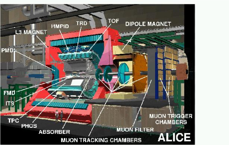
Figure 56: Schematic view of the ALICE detector.

The ALICE detector, shown in Fig. 56, is designed to cope with large particle multiplicities which, in central Pb+Pb collisions, are expected to be between 2000 and 8000 per unit rapidity at midrapidity. It consists of a central part, a forward muon spectrometer and forward/backward small acceptance detectors. The central part of ALICE consists of four layers of detectors placed in the small, $<0.5$ T, solenoidal field provided by the LEP L3 magnet. From the inner side to the outer side, these detectors are the Inner Tracker System (ITS), the large Time Projection Chamber (TPC), the Transition Radiation Detector (TRD) and the Time of Flight system (TOF). They provide charged particle identification in the pseudorapidity range $|\eta|<0.9$, with full azimuthal coverage and a broad $p_{T}$ acceptance. These large area devices are complemented by smaller acceptance detectors: the High Momentum Particle Identification (HMPID), the PHOton Spectrometer (PHOS) and the Photon Multiplicity Detector (PMD). In the forward/backward region, the charged multiplicity and the zero degree energy will be measured by additional detectors (T0, V0, FMD, ZDC) which will allow fast characterisation and selection of the events. Finally a forward muon spectrometer covering the pseudorapidity range $2.5<\eta<4$ is placed on the right side of the central part. It makes use of the usual techniques of muon identification at small angle and consists of a front absorber, a dipole magnet, ten high-granularity tracking chambers, a muon filter and four large area trigger chambers.

8.3 Accessible $x$ Range

The LHC can probe both the nucleon parton distribution functions, in $pp$ collisions, and their modifications in the nucleus, using heavy ion collisions, down to unprecedented low $x$ values where $x$ is the fraction of the nucleon momentum carried by the interacting parton. In this section, the $x$ range of heavy flavour production accessible to ALICE is quantitatively assessed.

The $x$ range probed depends on the center of mass energy per nucleon pair $\sqrt{s}$, the $Q\overline{Q}$ pair invariant mass, $M_{Q\overline{Q}}$, and on the pair rapidity, $y_{Q\overline{Q}}$. We consider the leading order process, $gg\rightarrow Q\overline{Q}$ in the collision of two ions with mass and charge $(A_{1},Z_{1})$ and $(A_{2},Z_{2})$. The square of the pair invariant mass is equal to the square of the center of mass energy of the initial gluons, $\hat{s}$,

$$M^{2}_{Q\overline{Q}}=\hat{s}=x_{1}\,x_{2}\,s=x_{1}\,\frac{Z_{1}}{A_{1}}\,x_{2}\,\frac{Z_{2}}{A_{2}}\,s_{\rm pp},$$ (77)

where $x_{1}$ and $x_{2}$ are the gluon momentum fractions and $s_{\rm pp}=(14~{}{\rm TeV})^{2}$ is the square of the $pp$ center of mass energy at the LHC. The longitudinal rapidity of the pair in the laboratory is given by:

$$y_{Q\overline{Q}}=\frac{1}{2}\ln\left[\frac{E+p_{z}}{E-p_{z}}\right]=\frac{1}{2}\ \ln\left[\frac{x_{1}}{x_{2}}\frac{Z_{1}A_{2}}{Z_{2}A_{1}}\right].$$ (78)

From the pair mass and rapidity, the dependence of $x_{1}$ and $x_{2}$ on $A$,$Z$, $M_{Q\overline{Q}}$ and $y_{Q\overline{Q}}$ can be derived, obtaining

$$x_{1}=\frac{A_{1}}{Z_{1}}\frac{M_{Q\overline{Q}}}{\sqrt{s_{\rm pp}}}\exp\left({y_{Q\overline{Q}}}\right)~{}~{}~{}~{}~{}~{}~{}~{}~{}~{}~{}~{}~{}~{}~{}~{}x_{2}=\frac{A_{2}}{Z_{2}}\frac{M_{Q\overline{Q}}}{\sqrt{s_{\rm pp}}}\exp\left({-y_{Q\overline{Q}}}\right).$$ (79)

We first focus on Pb+Pb and $pp$ reactions. At central rapidities, $x_{1}\simeq x_{2}$ with the magnitude determined by the ratio $M_{Q\overline{Q}}/\sqrt{s}$. The $x$ values for $Q\overline{Q}$ production at threshold, $M_{c\overline{c}}=2m_{c}=2.4$ GeV and $M_{b\overline{b}}=2m_{b}=9$ GeV, are given in Table 25.

Table 25: The $x$ values for $Q\overline{Q}$ pair production at threshold for central rapidities in Pb+Pb and $pp$ collisions.

system ($\sqrt{s}$)	$x$ $(c\overline{c})$	$x$ $(b\overline{b})$
Pb+Pb (5.5 TeV)	$4.3\times 10^{-4}$	$1.6\times 10^{-3}$
$pp$ (14 TeV)	$1.7\times 10^{-4}$	$6.4\times 10^{-4}$

Because of the lower mass, charm probes smaller $x$ values than bottom. The capability for charm and bottom measurements in the forward rapidity region, $y\simeq 4$, gives access to $x$ regimes about 2 orders of magnitude lower, down to $x\sim 10^{-6}$.

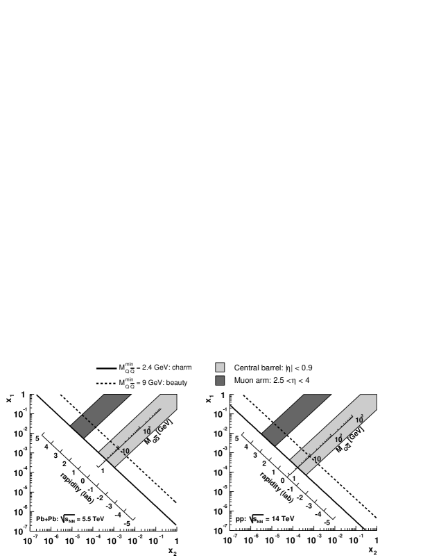
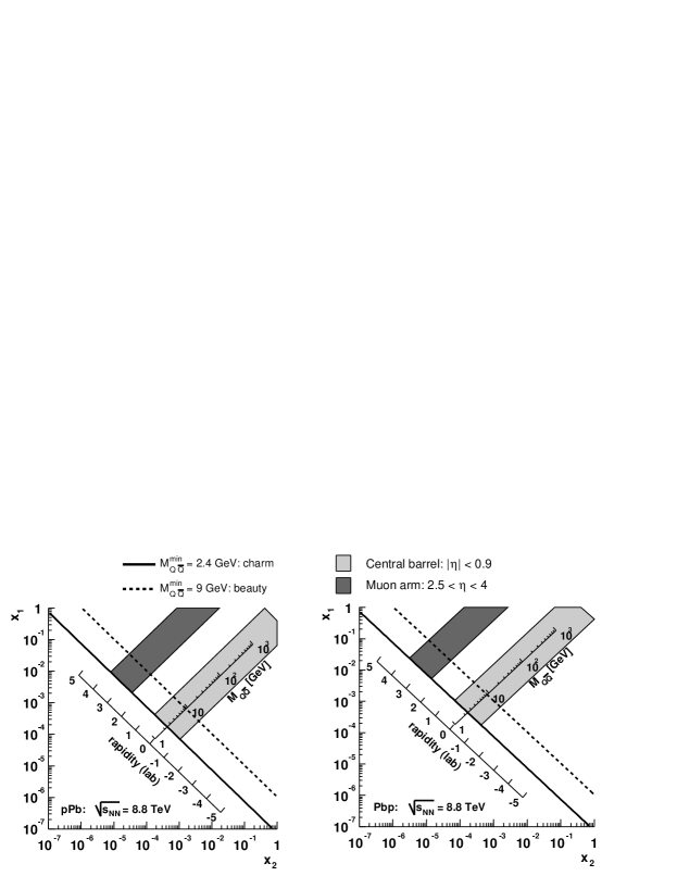
Figure 57: ALICE heavy flavour acceptance in the ($x_{1}$, $x_{2}$) plane for Pb+Pb (left) and $pp$ (right) collisions.

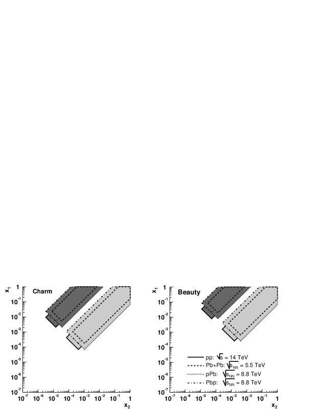
Figure 58: ALICE heavy flavour acceptance in the ($x_{1}$, $x_{2}$) plane for $p$Pb (left) and Pb$p$ (right) collisions.

Figure 59: Compiled ALICE acceptance in the ($x_{1}$, $x_{2}$) plane for charm (left) and bottom (right) in $pp$, Pb+Pb, $p$Pb and Pb$p$ collisions.

In Fig. 59, the regions of the ($x_{1}$, $x_{2}$) plane for charm and bottom measurements in the ALICE acceptance are shown for Pb+Pb collisions at 5.5 TeV and $pp$ collisions at 14 TeV. In this plane, points of constant invariant mass lie on hyperbolae, $x_{1}=M^{2}_{Q\overline{Q}}/(x_{2}\,s)$, which are straight lines on the log-log scale. The solid and dashed lines correspond to $c\overline{c}$ and $b\overline{b}$ pair production at threshold. Points with constant rapidity lie on straight lines, $x_{1}=x_{2}\exp(-2y_{Q\overline{Q}})$. The shaded regions show the acceptance of the ALICE central barrel, $|\eta|<0.9$, and of the muon arm, $2.5<\eta<4$.

In the case of asymmetric collisions, $Z_{1}\neq Z_{2}$ and $A_{1}\neq A_{2}$, the $Q\overline{Q}$ rapidity is shifted by:

$$\Delta y_{Q\overline{Q}}=\frac{1}{2}\,\ln\left(\frac{Z_{1}A_{2}}{Z_{2}A_{1}}\right)\,\,,$$ (80)

as seen in Eq. (78). For $p$Pb (Pb$p$) collisions, $\Delta y=+0.47~{}(-0.47)$. Therefore, combining $p$Pb and Pb$p$ runs will allow the largest $x_{1}$ and $x_{2}$ coverage with the central barrel and the muon arm. Figure 59 shows the $p$Pb and Pb$p$ acceptances while Fig. 59 compares the $pp$, Pb+Pb, $p$Pb and Pb$p$ coverages for charm (left) and beauty (right).

Note that these figures only give a qualitative idea of the $x$ regions accessible to ALICE since the leading order definitions of $x$ were used and the rapidity cuts were applied to the $Q\overline{Q}$ pair and not the detected particles. In addition, no minimum $p_{T}$ cuts were applied. Such cuts increase the minimum accessible value of $M_{Q\overline{Q}}$, correspondingly increasing the minimum accessible $x$. These approximations, however, are not too drastic since there is a very strong rapidity correlation between the initial $Q\overline{Q}$ pair and the produced heavy flavour hadrons and, as shown in the following sections, the minimum $p_{T}$ cut will be quite low, lower than the hadron mass, for most of the channels studied at ALICE.

8.4 Muons

The ALICE forward muon spectrometer is designed to detect heavy quarkonia in the $\mu^{+}\mu^{-}$ decay channel. The $\mu^{+}\mu^{-}$ continuum will be measured together with the resonances allowing the study of open charm and open bottom.

8.4.1 Quarkonia

Muons are detected in the pseudo rapidity interval $2.5<\eta<4$. To eliminate the huge low-$p_{T}$ background from $\pi$ and $K$ decays, a muon $p_{T}$ threshold is applied to single muons at the trigger level. The resulting geometrical acceptance is shown in Fig. 60 for $J/\psi$ and $\Upsilon$.

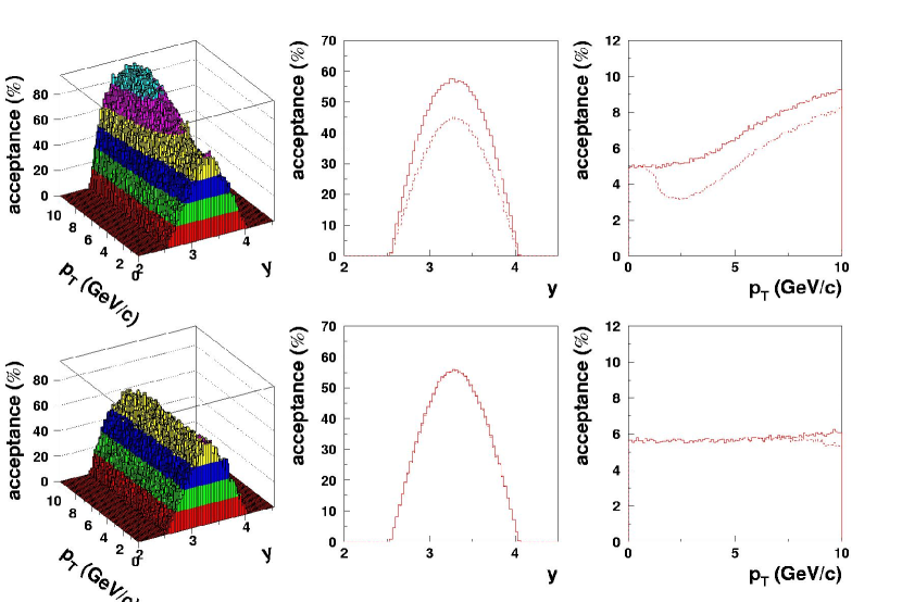
Figure 60: Geometrical acceptance for $J/\psi$ (top) and $\Upsilon$ (bottom). The left panels show the geometrical acceptance versus rapidity and transverse momentum. The middle and right panels show the acceptance as a function of rapidity and transverse momentum, respectively. In the middle and right panels, the acceptance is shown without (solid histograms) and with (dashed histograms) the trigger cut on single muon $p_{T}$. From Ref. [224].

The projection of the 3-D plots on the $y$ and $p_{T}$ axes are shown in the middle and right panels of the same figure. Together with these projections, the ones obtained after applying a sharp $p_{T}$ cut of 1 (2) GeV/$c$ for $J/\psi$ ($\Upsilon$) are also shown to give an idea of the trigger effects. As can be seen, only the $J/\psi$ acceptance is slightly affected by the trigger $p_{T}$ cut, implying that $J/\psi$ and $\Upsilon$ can be detected down to $p_{T}=0$.

An important characteristic of the spectrometer is that its mass resolution is expected to be of about $70$ ($100~{}{\rm MeV}/c^{2}$) for $J/\psi$ ($\Upsilon$). As shown in Fig. 61, such resolution allows separation of the $\Upsilon$ states. It should then be possible to disentangle scenarios of quarkonium suppression by studying the $p_{T}$ dependence of quarkonium ratios [29].

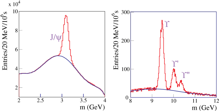
Figure 61: Opposite sign dimuon mass spectra in the region $2<m<4~{}{\rm GeV}$ (left) and $8<m<12~{}{\rm GeV}$ (right) for the $10\%$ most central Pb+Pb reactions. The spectra were obtained by means of fast simulations including acceptance cuts and detector efficiencies and resolutions. They correspond to a luminosity of $5\times 10^{26}~{}{\rm cm}^{-2}{\rm s}^{-1}$ and a running time of $10^{6}~{}{\rm s}$. From Refs. [233, 234].

The statistics expected in a $10^{6}$ s run, roughly corresponding to one month of data taking, are summarized in Table 26 for different colliding systems. (Note that since Ca has been replaced by Ar in the list of accepted nuclei, the Ca+Ca results are indicative of the expected rates for an intermediate mass system.) The signal-to-background ratios and the significances for detecting the various resonances are also given. We note that these numbers were obtained by applying analysis cuts which are not fully optimized. Therefore they should be considered as indicative numbers only. All numbers refer to primary production of the resonances and do not include any specific in-medium effects such as enhancement or suppression mechanisms. The total quarkonium production cross sections in proton-proton collisions were taken from Ref. [20]. These cross sections have been scaled to central ($10\%$) nucleus-nucleus reactions according to $A^{2}/(2\cdot 2)$ where the factors of $2$ represent the reduction for central relative to minimum bias collisions and nuclear shadowing [233]. The $p_{T}$ distributions have been parameterized according to CDF results (see Ref. [233] for more details).

Table 26: Expected background and signal rates, signal-to-background ratios and significance in pp and in central Pb+Pb and Ca+Ca collisions for charmonium and bottomonium. The numbers correspond to an interval of $\pm 1\sigma$ around the resonance mass. All rates and ratios are for a $10^{6}$s run. The luminosities for the Pb+Pb, Ca-Ca and pp system are $5\times 10^{26}$, $1\times 10^{29}$ and $1\times 10^{31}~{}{\rm cm}^{-2}{\rm s}^{-1}$, respectively. From Ref. [233].

system	state	B ($\times 10^{3}$)	S ($\times 10^{3}$)	S/B	S/$\sqrt{\rm S+B}$
	$J/\psi$	320	230	0.72	310
	$\psi^{\prime}$	150	4.6	0.03	12
Pb+Pb	$\Upsilon$	0.25	1.8	7.1	39
	$\Upsilon^{\prime}$	0.22	0.54	2.5	19
	$\Upsilon^{\prime\prime}$	0.18	0.26	1.5	12
	$J/\psi$	760	2000	2.7	1200
	$\psi^{\prime}$	360	41	0.11	64
Ca+Ca	$\Upsilon$	1.5	16	10.7	120
	$\Upsilon^{\prime}$	1.3	4.8	3.6	61
	$\Upsilon^{\prime\prime}$	1.1	2.3	2.0	39
	$J/\psi$	64	850	13	890
	$\psi^{\prime}$	32	17	0.53	76
$pp$	$\Upsilon$	0.49	6.5	13	78
	$\Upsilon^{\prime}$	0.45	2.0	4.4	40
	$\Upsilon^{\prime\prime}$	0.38	0.94	2.5	26

As shown in the table, the high statistics expected for $J/\psi$ will permit detailed studies as a function of both $p_{T}$ and centrality. It is then also possible to investigate the azimuthal distribution of $J/\psi$ with respect to the reaction plane [235]. For the $\Upsilon$, the statistics are obviously reduced but are nevertheless sufficient to investigate the $p_{T}$ and centrality dependence. Note particularly the large expected signal-to-background ratio (about 10) and good significance.

8.4.2 Open Charm and Open Bottom

The muon spectrometer should allow measurements of the open bottom cross section. This is possible because the background muons from $\pi$ and $K$ decay surviving the 1 GeV/$c$ trigger $p_{T}$ cut, as well as those coming from charm decay, can be efficiently removed with a higher software $p_{T}$ cut. In fact, as illustrated in Fig. 62, when applying a $p_{T}$ cut of $3~{}{\rm GeV}/c$ on each muon, the correlated signal from bottom decays represent a significant fraction of the total dimuon yield both at low ($1<m<3~{}{\rm GeV}$) and high ($6<m<9~{}{\rm GeV}$) invariant mass. Therefore, after subtraction of the uncorrelated combinatorial background (evaluated, for instance, by event mixing) from the total dimuon yield, one should be able to extract the unlike-sign correlated bottom decay signal in these two invariant mass regions.

It is important to note that the unlike-sign correlated signal from bottom decay has two different origins. In the high invariant mass region (Fig. 62, right) each muon comes from the direct decay of a $B$ meson. In the low invariant mass region (Fig. 62, left), the correlated signal from bottom is dominated by the so-called $B$-chain channel where both muons come from the decay of a single $B$ via a $D$. This implies that the bottom cross section can be estimated independently (at least to some extent) by a study of the low and high invariant mass regions. Note that similar measurements of the charm cross section should be achievable with appropriate analysis strategies.

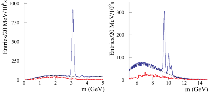
Figure 62: Opposite sign dimuon mass spectra in the region $0<m<5~{}{\rm GeV}$ (left) and $5<m<15~{}{\rm GeV}$ (right) for central Pb+Pb reactions. A $p_{T}$ threshold of $3~{}{\rm GeV}/c$ is applied on each single muon. The upper and lower histogram correspond to the total combinatorial background and to the correlated signal from bottom decay, respectively. The spectra were obtained by means of fast simulations. From Ref. [236].

In addition, it is important to remark that the bottom cross section can be also determined from the like-sign dimuon yield. In fact, $B$ meson oscillation as well as specific $B$ meson decay chains represent a source of correlated like-sign muon pairs. This component can be extracted by subtracting the uncorrelated signal from the like-sign spectrum [237].

Note finally that the open heavy flavor cross sections can also be extracted from the single muon spectra, as recently shown by the PHENIX collaboration with single electron spectra [148].

8.5 Electrons

The electrons, measured in the central region, will also give access to heavy quarkonia together with open charm and open bottom from the dielectron continuum. The key detector is the TRD which provides electron identification for $p_{T}>1$ GeV/$c$ and an electron trigger for $p_{T}>3$ GeV/$c$. It is operated in conjunction with the other ALICE central detectors for precise momentum measurements. In addition, the vertex capabilities of the ITS can distinguish between primary and secondary $J/\psi$. While the identification of the primary $J/\psi$ is of crucial importance for QGP studies, the identification of secondary $J/\psi$ can lead to a direct measurement of the $B$ meson production cross section. Furthermore, single high-$p_{T}$ electrons with displaced vertices give access to the inclusive heavy flavor cross sections.

8.5.1 Quarkonia

The $J/\psi$ and $\Upsilon$ acceptances in the dielectron channel are displayed in Fig. 63. The effects of the TRD-L1 trigger, simulated by requiring a sharp $p_{T}$ threshold of 3 GeV/$c$ on both decay electrons, are shown in the middle and right panels of the figure.

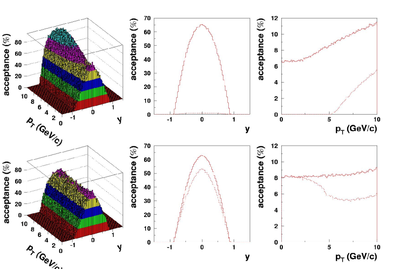
Figure 63: Same as Fig. 60 for the $J/\psi$ (top) and $\Upsilon$ (bottom) in the dielectron channel.

The effects of the $p_{T}$ cut on the $\Upsilon$ are similar to those observed for the $J/\psi$ in the dimuon channel, see Fig. 60. The cuts have a much stronger effect on the $J/\psi$ distribution. It is only at rather large $p_{T}$ that the decay kinematics allow both electrons to have $p_{T}>3~{}{\rm GeV}/c$. Therefore, while the $\Upsilon$ can be measured down to $p_{T}=0$, there is no $J/\psi$ acceptance below $p_{T}\sim 5.2$ GeV/$c$ because of the trigger condition. As in the case of the dimuon channel, the expected mass resolution is of the order of $100~{}{\rm MeV}/c^{2}$ for the $\Upsilon$ when the L3 magnet is operated at ${\rm B}=0.4~{}$T, allowing the $\Upsilon$ states to be separated.

The expected statistics are strongly dependent on the trigger efficiency which decreases with particle multiplicity. In the worst case anticipated for Pb+Pb, $dN_{\rm ch}/d\eta=8000$, the expected number of $\Upsilon$ per month is $\sim 2600$ in minimum-bias collisions. This number is expected to be significantly larger for lower charged particle multiplicities [238].

The current $J/\psi$ simulations indicate that the statistics will be significantly lower than that achieved in the dimuon channel, mainly due to the high $p_{T}$ cut of the electron trigger. In a scenario with a smaller charged particle multiplicity, the electron trigger $p_{T}$ threshold could be lowered, leading to better $J/\psi$ detection efficiency.

8.5.2 Open Charm and Open Bottom

The same studies described in section 8.4.2 for the muon channel will be also carried out in the electron channel using similar methods. In addition, the electron identification in the TRD can be used with the very good vertexing capabilities provided by the ITS. Due to the finite $c\tau$ of $D$ and $B$ mesons, their decay electrons have impact parameters d0 $\simeq 100-300~{}\mu{\rm m}$ and d0 $\simeq 500~{}\mu{\rm m}$, respectively. Figure 64 shows the resolution of the track position at the vertex achieved in ALICE (left) and the d0 distributions for electrons coming from $D$ and $B$ mesons and from other parent particles (right). The expected rates (per unit rapidity at midrapidity) for semileptonic decays of $D$ and $B$ mesons in central Pb+Pb collisions (5% $\sigma_{\rm tot}$) at $\sqrt{s}=5.5~{}{\rm TeV}$ are 2 and 0.09 per event, respectively.

The performance of ALICE for open bottom detection in the $B\rightarrow e+X$ channel has been studied using a detailed simulation of the apparatus and including all relevant background sources (direct-charm decays, pair production due to photon conversion in the detector materials, Dalitz decays of light and strange mesons, pions misidentified as electrons) [239]. A very pure electron sample is obtained using the transition radiation technique (TRD) in conjunction with the $dE/dx$ measurement in the TPC. The fraction of pions misidentified as electrons is $\sim 10^{-4}$. The electrons from $B$ decays have harder $p_{T}$ spectra and, as already mentioned, broader d0 distributions. Therefore, a sample of electrons from open bottom decays can be selected using suitable $p_{T}$ and d0 thresholds. The left-hand side of Fig. 65 presents the signal/(signal+background) ratio for three values of the electron $p_{T}$ cut as a function of the d0 threshold. As an example, a condition of $p_{T}>2$ GeV/$c$ and d0 $>180~{}\mu{\rm m}$ gives a sample of $90~{}\%$ purity. The expected number of $B$ mesons detected in $10^{7}$ central Pb+Pb events (1 month of ALICE data taking) is $\simeq 80000$ without any specific electron trigger. A more complete view of the attainable statistics is shown on the right-hand side of Fig. 65 as a function of the d0 threshold for three different $p_{T}$ thresholds.

If the $p_{T}$ and d0 thresholds are lowered to $\sim 1$ GeV/$c$ and $\sim 100~{}\mu{\rm m}$, the contribution of electrons from open charm decays becomes comparable with that of open beauty. A method for disentangling the two contributions is currently under study.

The second way to measure the open bottom cross section is based on the measurement of secondary $J/\psi$’s from $B$ decays. These secondary $J/\psi$’s are produced at large distances from the primary vertex and can therefore be selected by identifying $e^{+}e^{-}$ pairs with displaced vertices, as shown on the left-hand side of Fig. 66. The resulting invariant mass spectrum is presented on the right-hand side of Fig. 66.

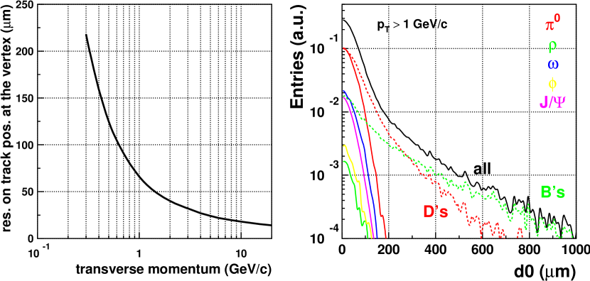
Figure 64: Left: the transverse momentum dependence of the bending projection (d0) of the impact parameter resolution. Right: the d0 distribution of electrons originating from different parent particles. From Ref. [240].

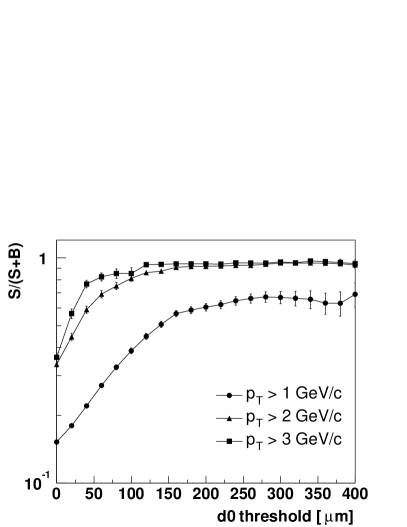
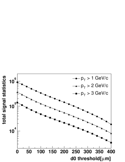
Figure 65: Detection of $B\rightarrow e+X$: ${\rm S/(S+B)}$ ratio (left) and signal statistics for $10^{7}$ central Pb+Pb events (right) as a function of the d0 threshold and for three values of the $p_{T}$ threshold. From Ref. [239].

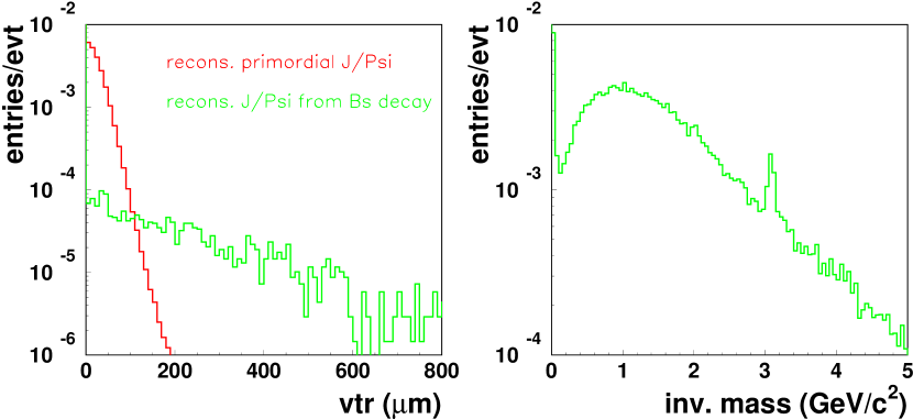
Figure 66: Left: dependence of the $J/\psi$ signal on the distance to the primary vertex. Right: invariant mass distribution of pairs with displaced vertices. From Ref. [240].

8.6 Electron-Muon Coincidences

The correlated $c\overline{c}$ and ${b}\overline{b}$ cross sections can be measured in ALICE using opposite sign electron-muon pairs. The electron is identified in the central part and the muon is detected in the forward muon spectrometer. This channel is the only leptonic channel that gives direct access to correlated ${c}\overline{c}$ and ${b}\overline{b}$ pairs. Indeed, in contrast to the $e^{+}e^{-}$ and $\mu^{+}\mu^{-}$ channels, resonance decays, direct dilepton production and thermal production cannot produce correlated $e\mu$ pairs. Within ALICE, the $e\mu$ channel has the additional advantage that the rapidity distribution of the corresponding signal extends in $1<y<3$, bridging the central and the forward acceptances [137]. Measurements of $e\mu$ coincidences were successful in $pp$ interactions at $\sqrt{s}=60~{}{\rm GeV}$ [241] and in $pN$ interactions at $\sqrt{s}=29~{}{\rm GeV}$ [242]. They are planned for heavy ion collisions with the PHENIX detector at RHIC [243]. Preliminary simulations have shown that such measurements might be possible with ALICE [240, 244, 245].

8.7 Hadrons

In the central part of ALICE, heavy mesons and baryons can be fully reconstructed from their charged particle decay products in the ITS, TPC and TOF. Thus, not only their integrated yields, but also their $p_{T}$ distributions can be measured. The most promising open charm decay channel is $D^{0}\rightarrow K^{-}\pi^{+}$ (and its charge conjugate) with a branching ratio of $\sim 3.9$% and $c\tau=124~{}\mu{\rm m}$. The expected rates (per unit rapidity at midrapidity) for $D^{0}$ (and $\overline{D}^{0}$) mesons, decaying into $K^{\mp}\pi^{\pm}$ pairs, in the 5% most central Pb+Pb collisions at $\sqrt{s}=5.5~{}{\rm TeV}$ and in $pp$ collisions at $\sqrt{s}=14~{}{\rm TeV}$ are $5.3\times 10^{-1}$ and $7.5\times 10^{-4}$ per event, respectively.

This decay channel allows direct identification of the $D^{0}$ particles by computing the invariant mass of fully-reconstructed topologies originating from displaced secondary vertices. The left-hand side of Fig. 67 sketches the decay. The main feature of this topology is the presence of two tracks with impact parameters of order $100~{}\mu{\rm m}$.

The capabilities of the ALICE central barrel for $D^{0}$-meson searches have been investigated both for Pb+Pb collisions, see Refs. [224, 246, 247], and for $pp$ collisions. All the relevant background sources have been included in these studies, along with a detailed simulation of the detector response. In particular, for $pp$, the position of the interaction vertex will have to be reconstructed event-by-event using the tracks.

In Table 27 the statistics for signal, S, and background, B, per event and the signal-to-background ratio after reconstruction are presented. The only selection is on pair invariant mass, $|M_{K\pi}-M_{D^{0}}|<3~{}\sigma=36~{}{\rm MeV}$.

Table 27: Statistics for signal and background and signal-to-background ratio including only selection on pair invariant mass, $|M_{K\pi}-M_{D^{0}}|<3~{}\sigma=36~{}{\rm MeV}$.

system ($\sqrt{s}$)	S/event	B/event	S/B
Pb+Pb (5.5 TeV)	$1.3\times 10^{-1}$	$2.8\times 10^{4}$	$4.5\times 10^{-6}$
$pp$ (14 TeV)	$2.4\times 10^{-4}$	$1.1\times 10^{-1}$	$2.3\times 10^{-3}$

The most effective selection in order to extract the charm signal out of the large combinatorial background of opposite-charge track pairs is based on the requirement to have two tracks with large impact parameters and a good pointing of the reconstructed $D^{0}$ momentum to the collision point (i.e. the pointing angle $\Theta_{p}$ between the $D^{0}$ momentum and its flight-line should be close to 0, as shown on the left-hand side of Fig. 67). The selection strategy is described in detail in Refs. [224, 246, 247]. In Table 28 the statistics after selection, together with the signal-to-background ratio and the significance, are presented. The expected statistics are $\simeq 13000$ reconstructed $D^{0}$ in $10^{7}$ central Pb+Pb events and $\simeq 19000$ in $10^{9}$ $pp$ events. The (relatively) poorer quality of the $pp$ results is due to the larger error on the primary vertex position with respect to Pb+Pb.

Table 28: Statistics for signal and background, signal-to-background ratio and significance after selections. The significance is computed for the number of events collected in a one month run, $10^{7}$ for Pb+Pb and $10^{9}$ for $pp$.

system ($\sqrt{s}$)	S/event	B/event	S/B (%)	${\rm S}/\sqrt{{\rm S+B}}$
Pb+Pb (5.5 TeV)	$1.3\times 10^{-3}$	$1.2\times 10^{-2}$	11	37   ($10^{7}$ events)
$pp$ (14 TeV)	$1.9\times 10^{-5}$	$1.7\times 10^{-4}$	11	44   ($10^{9}$ events)

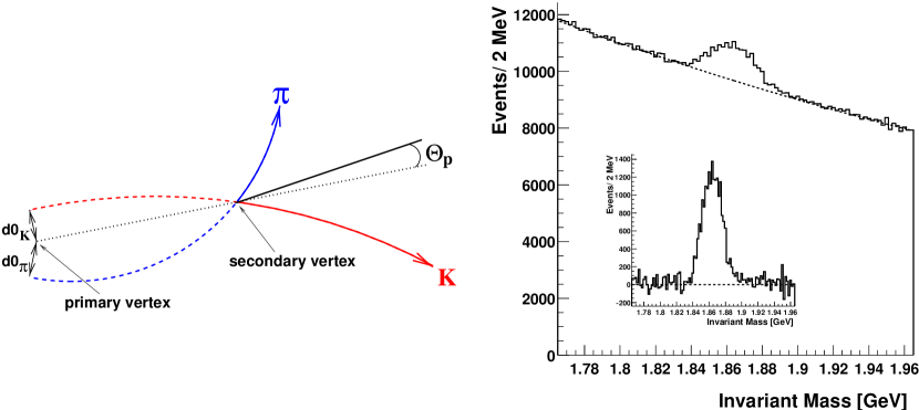
Figure 67: Left: schematic representation of the $D^{0}\rightarrow K\pi$ decay showing the impact parameters of the kaon (d0_K) and of the pion (d0_π) and the pointing angle ($\Theta_{\rm p}$). Right: $K\pi$ invariant mass distribution for $10^{7}$ central Pb+Pb events. The background-subtracted distribution is shown in the inset. From Ref. [247].

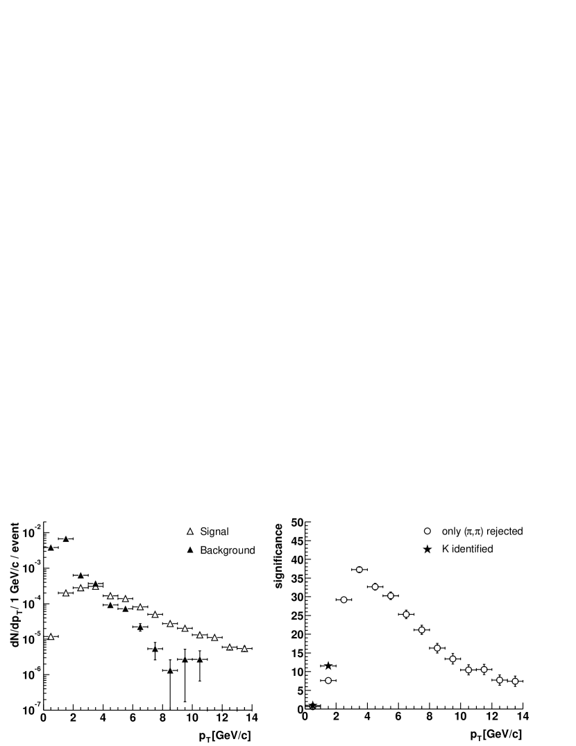
Figure 68: Left: the transverse momentum distribution of selected $D^{0}$ candidates in Pb+Pb collisions at $\sqrt{s}=5.5$ TeV. The signal and background are normalized to one central Pb+Pb event. Right: the corresponding significance for $10^{7}$ events. At low $p_{T}$ the values obtained requiring kaon identification are shown by the stars.

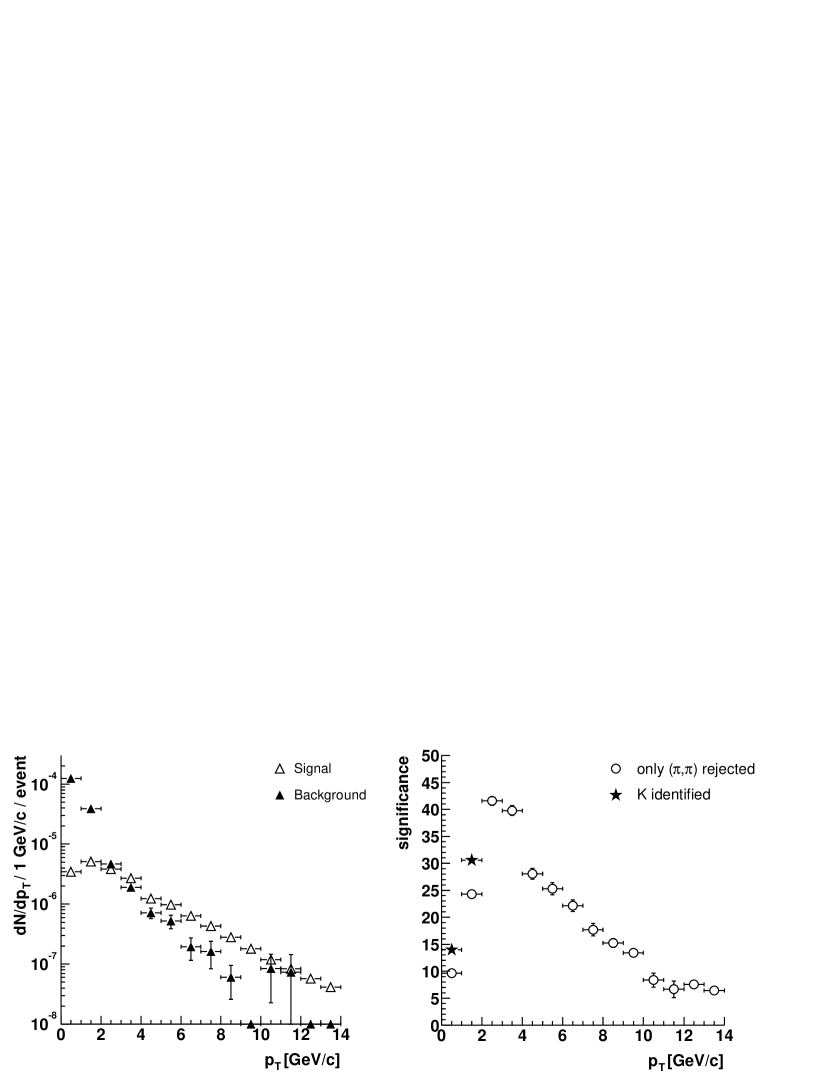
Figure 69: Left: the transverse momentum distribution of selected $D^{0}$ candidates in $pp$ collisions at $\sqrt{s}=14$ TeV. The signal and background are normalized to one minimum bias $pp$ event. Right: the corresponding significance for $10^{9}$ events. At low $p_{T}$ the values obtained requiring kaon identification are shown by the stars.

A typical example of the $D^{0}$ candidates invariant mass distribution in central Pb+Pb reactions, after selections, is shown on the right-hand side of Fig. 67 before and after background subtraction.

Figures 68 and 69 show the $p_{T}$ distribution of the signal and the background (normalized to one event) and the corresponding significance in Pb+Pb and $pp$ collisions respectively. Note that for $p_{T}\geq 7-8$ GeV/$c$, even if the simulated background statistics are insufficient, the significance is dominated by the signal statistics. The significance is larger than 10 for up to $p_{T}\approx 10$ GeV/$c$, both in Pb+Pb and in $pp$ collisions, if a 1 GeV/$c$ $p_{T}$ bin size is used. As shown in Ref. [247], the significance at low $p_{T}$ can be further improved by selecting sub-samples of $D^{0}$ candidates for which the kaon is identified. The values obtained with this method are shown with different symbols in Figs. 68-69. In this case the $D^{0}$ production cross section can be measured down to $p_{T}\simeq 1$ GeV/$c$ in Pb+Pb collisions and down to almost $p_{T}=0$ in $pp$ collisions.

8.8 Proton-nucleus Interactions

Proton-nucleus collisions are an important part of the ALICE physics program [224]. The main motivation is to bridge the results obtained in $pp$ and $AA$ interactions to unravel initial and final state medium effects.

More precisely, $pA$ studies of heavy flavour production will provide essential measurements of cold nuclear matter effects such as nuclear shadowing effects on heavy quarks [177] and nuclear absorption of quarkonium. Nuclear absorption effects have been demonstrated to be of crucial importance for disentangling “normal nuclear absorption” from “anomalous suppression” of quarkonium at the SPS [225, 226, 227]. Similarly, the $pA$ open charm and bottom yields will provide valuable references for the onset of thermal charm production in nuclear collisions and for the modification of the heavy flavour spectra due to energy loss in the QGP.

The ALICE $pA$ program, foreseen as dedicated $p$Pb, $d$Pb or $\alpha$Pb runs, is expected during the first few years of LHC operation [248]. As in $pp$ and $AA$ collisions, quarkonia and heavy flavor mesons will be measured through their (semi-)electronic decay channels in the ALICE central barrel. Also, $D$ mesons will be fully reconstructed using exclusive hadronic decay channels. The detector performance for $D^{0}\rightarrow K^{-}\pi^{+}$ (and charge conjugate) decays in $p$Pb collisions is expected to be similar to that of $pp$ since the multiplicity of background tracks will not be much larger than in $pp$ interactions. The asymmetric muon spectrometer allows all these studies in both direct and inverse kinematics since both $pA$ and “$Ap$” operation is, in principle, possible. Detailed simulations investigating the expected detector performance in $pA$ collisions are underway.

8.9 Run Plan

The present ALICE plans for data taking during the LHC heavy ion runs, in addition to participation in the 14 TeV $pp$ runs, are now briefly described, see Ref. [248] for more details. In the first 5-6 years of ion runs, we propose: 1-2 years Pb+Pb; 1-2 years Ar+Ar; and 1 year $p$Pb-like collisions ($p$Pb, $d$Pb or $\alpha$Pb). Later options depend on the outcome of the early runs: dedicated $pp$ or $pp$-like ($dd$ or $\alpha\alpha$) collisions; other $AA$ systems such as O+O, Kr+Kr or Sn+Sn; other $d(\alpha)A$ systems; or a low energy Pb+Pb run.

The maximum Pb+Pb luminosity for the ALICE central detectors is $L=10^{27}~{}{\rm cm}^{-2}{\rm s}^{-1}$, imposed by the pile-up event rate in the TPC and the DAQ bandwidth, 1 kHz, of the muon spectrometer. Nevertheless, to achieve better muon statistics, dedicated high luminosity runs of up to $L=2\times 10^{28}~{}{\rm cm}^{-2}{\rm s}^{-1}$ involving the muon spectrometer without the TPC could be foreseen with a high $p_{T}$ muon trigger, primarily for $\Upsilon$ decays.

To study the results as a function of energy density, at least one intermediate mass system, most likely Ar+Ar, will be studied in the first years. If more energy density points are needed, other systems such as Sn+Sn, Kr+Kr and O+O may be studied at a later stage. Luminosities similar to those used for the Pb+Pb runs will be used for the intermediate mass ion runs.

Although ALICE will take $pp$ data at 14 TeV in parallel with the other experiments, the luminosity must be reduced to $\approx 3\times 10^{30}~{}{\rm cm}^{-2}{\rm s}^{-1}$ to keep the pile up rate in the TPC and the ITS at an acceptable level. Higher luminosity runs with the muon spectrometer alone are possible with luminosities up to $5\times 10^{31}~{}{\rm cm}^{-2}{\rm s}^{-1}$.

In addition, lower energy $pp$ collisions, closer to the Pb+Pb center of mass energy, $5.5-7$ TeV, might be needed for reference data.

8.10 Summary

The capabilities of ALICE for heavy flavour physics at the LHC will provide a comprehensive understanding of open and hidden heavy flavour production at low $x$ where strong nuclear gluon shadowing is expected. The large number of accessible channels will permit detailed investigations of the properties of the nuclear medium. Open heavy flavour measurements will provide information on the primary production mechanisms, parton energy loss and possible secondary production of heavy quarks. The complete spectroscopy of the quarkonium states will be used to probe the deconfined medium and to pin down its temperature. The simultaneous measurement of open and hidden heavy flavours will provide a powerful tool to study quarkonium suppression/enhancement in the QGP. Thanks to the large acceptance of the detector, the signals will be reconstructed over a broad transverse momentum range. This is particularly important for establishing the reference production rates with high accuracy and to investigate the characteristics of the QGP. The measurements will be performed for a variety of heavy and light nucleus-nucleus systems as well as for $pp$ and $pA$ reactions. The latter are mandatory since, besides probing shadowing effects, they will provide the normalization for understanding the properties of the nuclear medium in $AA$ collisions.

In addition to the measurements discussed here, further exciting possibilities should be opened with, for example, the reconstruction of hadronic decays of charged $D$ and $B$ mesons, reconstruction of double charm baryons by combining hadronic and leptonic channels, and dilepton measurements at very high invariant mass.

9 QUARKONIA AND HEAVY FLAVOUR DETECTION WITH THE CMS DETECTOR 

9.1 Introduction

The interest in quarkonium production at the LHC emerged from the CERN SPS results [249, 225] which showed a strong anomalous suppression in $J/\psi$ production in Pb+Pb collisions at $\sqrt{s}=17.3$ GeV. RHIC will study $J/\psi$ production and suppression in detail at $\sqrt{s}=200$ GeV since the temperature of the system produced at RHIC should be high enough for direct $J/\psi$ suppression. Although the $\Upsilon$ production cross section is large enough to be observed at RHIC, albeit with limited statistics, its suppression is not expected until the higher initial temperatures at the LHC are reached. CMS is particularly well suited to study the $\Upsilon$ family, the continuum up to the $Z^{0}$ mass and, to a lesser extent, the $J/\psi$ and $\psi^{\prime}$.

Open heavy flavour production is important for studying the behaviour of massive colour charges in a dense medium at the LHC. The charm and bottom production cross sections are much larger than at RHIC. Systematics studies of heavy flavours, especially $B$ mesons, can be performed with CMS. In particular, in-medium gluon radiation and collisional energy loss of heavy quarks can result in the suppression and modification of the high-mass dilepton [137, 250, 251] and secondary $B\rightarrow J/\psi$ decay spectra [250, 251]. Finite quark mass effects can suppress medium-induced radiation of heavy quarks, enhancing e.g. the $B/\pi$ ratio [147].

We briefly describe the CMS detector in section 9.2. Then we provide the resonance cross sections and the background description used in our simulations in section 9.3. Section 9.4 describes the detector response, the acceptance and the dimuon reconstruction algorithm. The results of the simulations are presented in section 9.5, including the signal/background ratios and the dimuon invariant mass distributions. In the last section, 9.6, the CMS capabilities for open heavy flavour and $Z^{0}$ measurements in the mass range above the $\Upsilon$ are discussed.

9.2 The CMS Detector

The CMS detector is designed to identify and measure muons, electrons, photons and jets over a large energy and rapidity range. It offers the widest muon acceptance centered at midrapidity. CMS is particularly well suited to study the $\Upsilon$ family, the continuum up to the $Z^{0}$ mass and, to a lesser extent, the $J/\psi$ and $\psi^{\prime}$. The CMS dilepton capability allows systematic studies of heavy flavour physics. The impact parameter (centrality) of the collision can be determined from measurements of transverse energy production over the range $|\eta|$ $<$ 5.

CMS has a high-field solenoidal magnet with a uniform 4 T field, leading to a compact detector. The first absorber, the electromagnetic calorimeter, is 1.3 m from the interaction point, eliminating a large fraction of the hadronic background. The powerful tracking system provides good track reconstruction efficiency for dimuons even for very large charged particle densities, $dN_{\rm ch}/dy\leq$ 8000, providing excellent dimuon mass resolution.

A detailed description of the detector elements can be found in the corresponding Technical Design Reports [252, 253, 254, 255]. A longitudinal view of the detector is shown in Fig. 70. The central element of CMS is the magnet, a 13 m long, 6 m diameter, high-field solenoid with an internal radius of $\approx$3 m. The tracker and muon chambers cover the pseudorapidity region $|\eta|<2.4$, while the ECAL and HCAL calorimeters reach $|\eta|=3$. A pair of quartz-fiber very forward (HF) calorimeters, located $\pm 11$ m from the interaction point, cover the region $3<|\eta|<5$ and complement the energy measurement. The tracker is composed of pixel layers and silicon strip counters. The barrel part of tracker, $|\eta|<0.8$, consists of three pixel layers 4, 7, and 11 cm radially from the beam line and 9 layers of silicon strip counters. The endcap part of tracker, $\eta>0.8$, is more complex. There are two pairs of pixel layers symmetrically located 34 cm and 45 cm from the geometrical center of the detector. Outside this, two symmetric sets of 12 silicon layers are situated up to 265 cm from the center of the detector. The electromagnetic calorimeter is made of almost 83000 scintillating PbWO₄ crystals. The hadronic calorimeter consists of scintillator inserted between copper absorber plates.

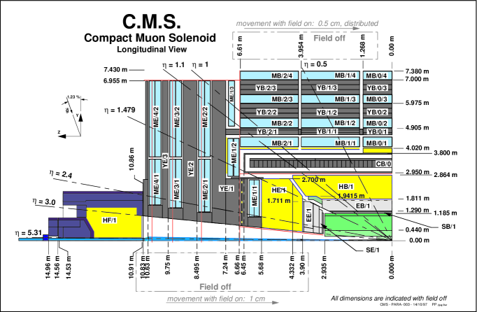
Figure 70: A longitudinal view of the CMS detector.

The CMS muon stations consist of drift tube chambers (DT) in the barrel region (MB), $|\eta|<1.2$, cathode strip chambers (CSCs) in the endcap regions (ME), $0.9<|\eta|<2.4$, and resistive plate chambers (RPCs) in both barrel and endcaps, for $|\eta|<1.6$. The RPC detector is dedicated to triggering, while the DT and CSC detectors, used for precise momentum measurements, also have the capability to self-trigger up to $|\eta|<2.1$. The muon system can thus reconstruct muons in the range $|\eta|<2.4$.

In each of the 12 sectors of the barrel return yoke of the magnet (YB), covering $30^{\circ}$ in azimuthal angle $\phi$, there are four muon barrel ‘stations’, MB$i$, $i=1,4$ in Fig. 70. Each station consists of one DT and one (or two, in the two innermost stations) RPC chambers. In each DT chamber, there are two ”superlayers” of four DT planes measuring the $(r,\phi)$ coordinates in the bending plane and another superlayer measuring the $z$ coordinate. In the outermost station, MB4, there are only two $(r,\phi)$ superlayers. Thus a muon traversing the whole barrel has 44 measurement points (‘hits’) in the DT systems and 6 hits in the RPC. There are a total of 240 stations in the barrel system. Each endcap region has four muon stations of CSCs. Each chamber gives six measurements of the $\phi$-coordinate (strips) and six measurements of the $r$-coordinate (wires). RPCs will be added in the barrel and endcaps to provide an additional trigger. Six layers of RPCs will be mounted in the barrel chambers and four in the endcaps.

9.3 $AA$ Collisions

9.3.1 Resonance cross sections

We use the quarkonium cross sections per nucleon calculated in section 3.2 in our simulations. The calculations, performed in the CEM, include nuclear shadowing but do not include absorption by nucleons and secondaries since the interplay between shadowing and absorption as a function of $\sqrt{s}$ is unknown. For convenience, the inclusive $AA$ dimuon cross sections given in Tables 9 and 10 are reproduced in Table 29.

Table 29: Total cross sections for quarkonium production in minimum bias $AA$ collisions.

System	Pb+Pb	Sn+Sn	Kr+Kr	Ar+Ar
$\sqrt{s}$ (TeV/nucleon)	5.5	5.84	6.14	6.3
Resonance	$B_{\mu\mu}$ $\sigma_{AA}$ ($\mu$b)
$J/\psi$	48930	17545	9327	2321
$\psi^{\prime}$	879	315	167.6	41.7
$\Upsilon$	304	108.1	57.4	13.8
$\Upsilon^{\prime}$	78.8	28	14.8	3.6
$\Upsilon^{\prime\prime}$	44.4	15.8	8.4	2.0

9.3.2 Background and kinematic distributions

Soft hadronic background.

Soft hadron production is the main dimuon background. This background is estimated from the charged particle multiplicity and the shape of the pion and kaon transverse momentum distributions.

The charged particle multiplicity, $dN_{\rm ch}/d\eta$, is unknown for the LHC energies. Early estimates of this multiplicity in central collisions ($b=0$) and midrapidity ($\eta=0$) were as high as 8000 for Pb+Pbcollisions [256]. In contrast, the first extrapolations from RHIC suggested that the Pb+Pb multiplicity could be as low as 2000 [165]. We choose two values for our simulations: 2500 (low) and 5000 (high). Lower multiplicities reduce the dimuon background. The track reconstruction algorithm was designed to function for a multiplicity of 8000, so that the current, lower, estimates should result in higher reconstruction efficiencies. The high and low values of the multiplicities used in the simulations are shown in Table 30. The upper numbers for each set correspond to the 5% most central collisions, assuming the multiplicity scales as $A^{4/3}$ from Pb+Pb. The lower numbers for each set correspond to collisions at $b=0$. In this case, the multiplicity can be higher.

Table 30: The high and low multiplicity sets, $dN_{\rm ch}/d\eta|_{\eta=0}$, used in the simulations. In both cases, the results are shows for the 5% most central collisions and impact parameter $b=0$.

		$dN_{\rm ch}/d\eta|_{\eta=0}$
Set		Pb+Pb	Sn+Sn	Kr+Kr	Ar+Ar
High	5% most central	5000	2400	1500	550
	$b=0$	7500	4000	2600	850
Low	5% most central	2500	1200	750	280
	$b=0$	3800	1900	1300	450

The soft hadronic background is assumed to entirely consist of pions and kaons produced according to the ratio $K/\pi=0.12$, independent of $b$. We use the SHAKER algorithm [257] to simulate the pion and kaon momentum distributions where $\langle p_{T}\rangle_{\pi}=0.47$ GeV/$c$ and $\langle p_{T}\rangle_{K}=0.67$ GeV/$c$. We note that HIJING [215, 216] produces pions and kaons with lower momenta, $\langle p_{T}\rangle_{\pi}=0.43$ GeV/$c$ and $\langle p_{T}\rangle_{K}=0.52$ GeV/$c$. Due to the magnetic field, only muons with $p_{T}>3.5$ GeV/$c$ will reach the barrel muon chambers. This minimum momentum requirement serves as the primary background rejection criteria. More than 99.8% of the SHAKER hadron background is rejected. The lower average momentum of HIJING reduces the probability for acceptance of decay muons by a factor of two with respect to SHAKER. Track reconstruction will also be an effective method of background rejection.

Heavy flavour decays.

The other important source of quarkonium background is $Q\overline{Q}$ pair production and decay. The number of pairs produced in $AA$ collisions as a function of impact parameter $b$ is

$$N(Q\overline{Q})=\sigma(Q\overline{Q})T_{AA}(b)\,\,,$$

directly proportional to the nuclear overlap function $T_{AA}(b)$ where $T_{\rm PbPb}(0)=30.4$/mb, $T_{\rm SnSn}(0)=13.3$/mb, $T_{\rm KrKr}(0)=8.5$/mb and $T_{\rm ArAr}(0)=2.9$/mb. The NLO $Q\overline{Q}$ production cross sections in 5.5 TeV $pp$ interactions are $\sigma(c\overline{c})=6.3$ mb and $\sigma(b\overline{b})=0.19$ mb (with large uncertainties – see section 2). Since the center of mass energies are higher for lighter ions, the $Q\overline{Q}$ cross sections per nucleon increase slightly from Pb+Pb to Ar+Ar interactions. The number of $Q\overline{Q}$ pairs at $b=0$ for the collision systems considered is shown in Table 31.

Table 31: Number of $Q\overline{Q}$ pairs produced at $b$=0.

	Pb+Pb	Sn+Sn	Kr+Kr	Ar+Ar
$c\overline{c}$	192	86	57	20
$b\overline{b}$	6	3	2	1

Although $N(c\overline{c})\gg N(b\overline{b})$, dimuons from $c\bar{c}$ decays are not the largest contribution to the background. Among all background sources taken into account, $b\bar{b}$ decays produce muons with the highest average transverse momentum, making a significant contribution to the background. The muon $p_{T}$ and $\eta$ distributions are extracted from PYTHIA [211] with $\langle$$p_{\rm T}^{\mu}$$\rangle$${}_{c}=0.51$ GeV/$c$ and $\langle$$p_{\rm T}^{\mu}$$\rangle$${}_{b}=1.2$ GeV/$c$.

Only 6% of single $b$ decays produce two muons and, of these, 2/3 are of opposite sign. When the CMS kinematic cuts, $p_{\rm T}^{\mu}>3.5$ GeV/$c$ and $|\eta|<2.4$, are included, more than 98% of the single $b$ decay muons do not survive the cuts. The probability of obtaining a dimuon from these decays after cuts is $\approx 10^{-4}$, shown in Table 32. About 80% of the accepted pairs are of opposite sign so that the correlated like-sign muon rate is negligible. Thus, to simplify the simulations, we assume that all muon pairs from $b\bar{b}$ decays are of opposite sign.

Table 32: The probability of $n$-muon signals in $b$ quark decays.

	0 $\mu$	1 $\mu$	2 $\mu$	3 $\mu$
before CMS cuts	0.626	0.308	0.060	0.006
after CMS cuts	0.987	0.0125	0.00018	0

9.4 Detector Response

9.4.1 Acceptances

The $p_{T}$ and $\eta$ distributions of the quarkonium sstates used in the simulations were obtained from several sources. The $p_{T}$ distributions of the three $\Upsilon(S)$ states were extrapolated from CDF data [258] while PYTHIA was used to generate the $\eta$ distributions. PYTHIA was also used to obtain the $J/\psi$ and $\psi^{\prime}$ distributions.

We assume that the primary vertex is at the geometrical centre of the detector. Each resonance decay muon is tracked through a 4 T magnetic field by GEANT [259] using the CMSIM package [260]. A dimuon is accepted if each decay muon of the pair passes through at least one muon chamber. We also introduce a $p_{T}$ cut of 3.5 GeV/$c$ for each muon, just above the minimum $p_{\rm T}^{\mu}$ needed to reach the first muon chambers in the barrel. This cut on $p_{\rm T}^{\mu}$ leads to very different resonance acceptances. The $J/\psi$ decay muons have $\langle$$p_{\rm T}^{\mu}$$\rangle=1.7$ GeV/$c$ so that only 0.8% of the $J/\psi$ decays give leptons above the muon threshold. On the other hand, the $\Upsilon$ decay muons have $\langle$$p_{\rm T}^{\mu}$$\rangle=4.6$ GeV/$c$ . Thus 40% survive the $p_{T}$ cut. The acceptances discussed below and shown in Fig. 71 are geometrical only. The dimuon reconstruction efficiencies, the trigger efficiency and the muon $p_{\rm T}$ cut are not taken into account.

The $\Upsilon$ acceptance is flat, $\approx 27$% in the full $\eta$ range of the detector before the muon $p_{T}$ cut, dropping to 16% once the muon $p_{T}$ cut is applied. With the barrel alone, the $\Upsilon$ acceptance is 13% before the $p_{T}$ cut and 9.5% after. The $p_{T}$ dependence of the accepted $\Upsilon$ in Fig. 71 does not change between the full detector and the barrel. The $p_{T}$ distribution starts from zero and is only statistically limited in the high-$p_{T}$ region, allowing a comparison between the high- and low-$p_{T}$ events.

The situation is different for the $J/\psi$. The integrated $J/\psi$ acceptance is about ten times lower than the $\Upsilon$ acceptance. There is an additional factor of 10 reduction when the $J/\psi$ acceptance is limited to the barrel due to the natural $p_{\rm T}^{\mu}$ cut provided by the material located in front of the muon chambers. Including a 3.5 GeV/$c$ cut diminishes the acceptance very strongly. Only muons from high $p_{T}$ $J/\psi$ decays ($p_{T}$ $J/\psi$ ¿ 4 GeV/$c$) can reach the barrel muon chambers, as clearly shown in Fig. 71. However, when the endcap regions are included can the $J/\psi$ be detected over the whole $p_{T}$ range. The acceptance is small but the expected rate is large.

Figure 71: The $p_{T}$ dependence of the dimuon acceptance for $J/\psi$ (upper) and $\Upsilon$ (lower) resonances. In each case both the full CMS detector (solid line) and the barrel only (dashed line) have been considered.

9.4.2 Track reconstruction

Pattern recognition and track reconstruction determine, to a large extent, the feasibility of heavy ion measurements with CMS. The particles were tracked through the detector using a full GEANT simulation. The tracks where followed down to 100 KeV for electromagnetic processes and 1 MeV for hadronic processes, an order of magnitude below the default GEANT energy threshold cuts. The quarkonium studies have has been carried out for a range of $dN_{\rm ch}/d\eta$, up to an extreme value of 8000, far beyond the present upper limit of 5000 for central Pb+Pb collisions. The upper limit of $dN_{\rm ch}/d\eta=8000$ led to occupancies of up to 18% for the 5 outermost Si-layers of the barrel, located more than 70 cm from the beam, and of 50% or more for the innermost Si-strip detectors. Occupancies of 2-4% [261] are expected for the pixel layers due to their very high granularity. Thus, the occupancies determine the number of layers used in the track-reconstruction algorithm.

The goal of the track-finding algorithm is to select pairs of muon tracks coming from the interaction point. In the barrel, the algorithm uses the two pixel layers at 7 and 11 cm and the four outermost Si-layers. This is the minimum combination necessary to get good efficiency and purity for high occupancy rates in the tracker. The usage of the third pixel layer at 4 cm is under investigation.

The vertex is determined from a combination of clusters in the pixel layers assuming the interaction occurs at the geometrical centre of the detector, $(0,0,0)$. Figure 72 shows the results of the interaction point vertex determination for a simulated collision at $z=5$ cm for $dN_{\rm ch}/d\eta=2500$ and 8000. The resolution is $\sigma_{z}=140$ $\mu$m.

The track finding algorithm starts from the muon chambers since they are the least populated planes. The tracks are propagated within roads in transverse ($R/z,\phi$) and longitudinal ($R,z$) planes with simple parameterizations $d\phi=k\,dr/p_{\rm T}$ for the barrel, $d\phi=k\,dz/p_{\rm L}$ for the endcaps, and a straight line in the ($R,z$) plane.

The track candidates are then fitted and, after vertex constraints, the best quality track is selected. Several dimuon events have been studied: homogeneous dimuons from $\Upsilon$ decays as well as mixed pairs originating from $\pi/K/b$ decays where one muon comes from a $\pi$ or $K$ decay and the other from a $b$ decay. For the moment, only barrel tracks have been investigated. In the region $|\eta|<0.8$, the efficiency of $\Upsilon$ reconstruction is $\approx$ 90% for $dN_{\rm ch}/d\eta=2500$ and 85% for 5000 with a purity above 99%. The $\Upsilon$ reconstruction efficiency is 76% for $dN_{\rm ch}/d\eta=8000$. The efficiency for $\pi$ and $K$ decays is about six times lower, leading to good background rejection. For $0.8<|\eta|<1.3$, the $\Upsilon$ efficiency is  50%. The high precision tracking leads to an excellent dimuon mass resolution of 46 MeV at the $\Upsilon$ peak when both tracks have $|\eta|<0.8$, increasing to 60 MeV when one track has $0.8<|\eta|<1.3$.

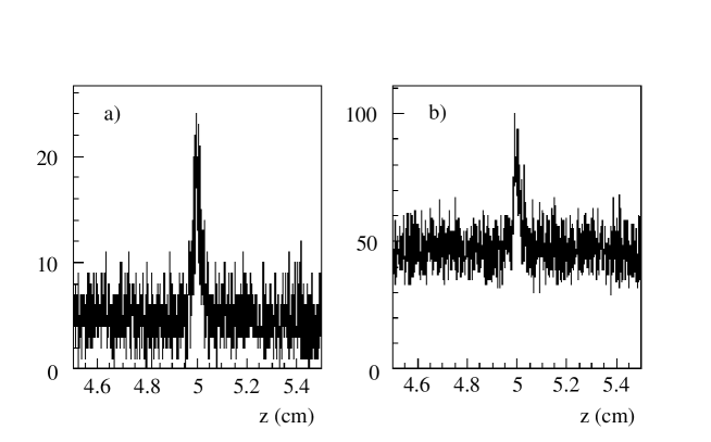
Figure 72: Distribution of the $z$ position of the primary vertex for $dN_{\rm ch}/d\eta$ of (a) 2500 and (b) 8000. The initial collision was generated at $x=y=5$ $\mu$m and $z=5$ cm.

9.5 Invariant Mass Spectra

9.5.1 Signal/background and mass distributions

The simulations are based on the weight method with acceptance tables. They consider combinations of muons with $p_{T}^{\mu}>3.5$ GeV/$c$. Either both muons originate from $\pi$ and/or $K$ decays, $hh$, or from $c\overline{c}$ and $b\overline{b}$ decays, or from a ”mixed source”, one from $\pi$ or $K$ decays and one from heavy quark decays, $hb$ and $hc$.

The invariant mass of each pair is calculated. Two mass regions are then defined, the $\Upsilon$ region, $8.5<M_{\mu\mu}<11$ GeV/$c^{2}$  and the $J/\psi$ region, $2<M_{\mu\mu}<4.5$ GeV/$c^{2}$ . The resulting invariant mass distribution is smoothed by a Gaussian with a width determined by the expected mass resolution.

The opposite sign dimuon invariant mass distributions obtained in Pb+Pb, Sn+Sn, Kr+Kr and Ar+Ar collisions are shown in Fig. 73 for the $J/\psi$ and in Fig. 74 for the $\Upsilon$. Using the high and low multiplicity sets given in Table 30, we present results for a one month run, $1.3\times 10^{6}$ seconds, assuming a 50% machine efficiency. The $J/\psi$ and $\Upsilon$ statistics are given in the figures and summarized in Table 33, assuming the average luminosities of Ref. [262]. The 18000 $\Upsilon$ measured in a one month Pb+Pb run are statistically significant enough to bin with impact parameter. Limiting detection to the barrel reduces the statistics, but not unacceptably for intermediate-mass ions.

The signal-to-background ratio, S/B, between the number of detected resonances, $J/\psi$ or $\Upsilon$(1S), and the number of opposite sign dimuons under the peak in the mass window $M_{\rm res}\pm 50$ MeV, is calculated from Fig. 73 for the $J/\psi$ and from Fig. 74 for the $\Upsilon$. This ratio depends on the multiplicity. Table 34 gives the S/B ratio for the $J/\psi$ and $\Upsilon$ and the significances, S/$\sqrt{\rm S+B}$, for the three $\Upsilon(S)$ states. The results are shown for both the high and low multiplicity sets of Table 30 for each collision system. The lower signal-to-background ratios and significances correspond to the larger background, high multiplicity set. The higher signal-to-background ratios and significances result from the reduced background of the low multiplicity set.

Table 33: The number of resonances detected in a one month, $1.3\times 10^{6}$ s, run in the full detector and in the barrel alone (in parentheses).

$N_{\rm res}/10^{3}$	Pb+Pb	Sn+Sn	Kr+Kr	Ar+Ar
$J/\psi$	24	160	360	1450
	(4.7)	(31)	(81)	(275)
$\Upsilon$	18	116	260	1020
	(7.9)	(51)	(114)	(450)
$\Upsilon^{\prime}$	5.4	35	80	310
$\Upsilon^{\prime\prime}$	3.4	22	50	195

Table 34: The signal-to-background ratios, S/B, and the significances, S/$\sqrt{\rm S+B}$ in the 5% most central collisions for the two multiplicity sets given in Table 30. The smaller numbers correspond to the high multiplicity set while the larger numbers are obtained with the low multiplicity set.

		Pb+Pb	Sn+Sn	Kr+Kr	Ar+Ar
S/B	$J/\psi$	0.2-0.5	0.4-1.1	0.7-1.8	2.0-6.8
	$\Upsilon$	0.4-0.9	0.7-1.9	1.5-4.3	5.3-15.6
	$\Upsilon$	69-93	220-276	396-460	925-978
S/$\sqrt{\rm S+B}$	$\Upsilon^{\prime}$	24-38	84-123	165-218	447-512
	$\Upsilon^{\prime\prime}$	16-26	55-86	113-157	325-391

Figure 75, corresponding to Pb+Pb collisions with the high  multiplicity set, shows the expected opposite sign dimuon mass distribution in the $\Upsilon$ mass region in more detail. The most important contributions to the background are given. The background is typically dominated by $\pi$ and $K$ decays in combination with each other, $hh$, or with a heavy quark decay, $hb$ and $hc$.

Although $N(b\overline{b})\ll N(c\overline{c})$, in an $AA$ collision the $b\overline{b}$ contribution is more important. The background is primarily from uncorrelated muon pairs. This background can be subtracted from the opposite sign spectrum using the ‘like-sign’ spectra, as done by the SPS NA50 collaboration [249, 225]. In this case, the signal is

$$N^{\rm Sig}=\ N^{+-}-2\sqrt{N^{++}\ N^{--}}$$

where $N^{+-},N^{++}$ and $N^{--}$ are the combinations of opposite sign pairs and positive and negative like-sign pairs respectively in a given mass interval. Figure 76 presents the mass distributions resulting from this subtraction.

Figure 73: The opposite sign dimuon invariant mass distributions in the $J/\psi$ mass region obtained in the 5% most central collisions in a one month run with the high multiplicity set (left) and low multiplicity set (right) as defined in Table 30.

Figure 74: The opposite sign dimuon invariant mass distributions in the $\Upsilon$ mass region obtained in the 5% most central collisions in a one month run with the high multiplicity set (left) and low multiplicity set (right) as defined in Table 30.

Figure 75: The invariant mass distribution in the $\Upsilon$ mass region of opposite sign dimuons, including the largest background contributions, with the high multiplicity set. For $hh$, both muons come from $\pi$ and $K$ decays. For $hb$ and $hc$, one muon is from $\pi$ or $K$ decay while the second is from a $b$ or $c$ decay. For $bb$, both muons come from $b\overline{b}$ decays.

Figure 76: The signal invariant mass distribution, after background subtraction, in $J/\psi$ (left) and $\Upsilon$ (right) mass regions obtained in one month with the high multiplicity in Pb+Pb collisions.

9.6 Open Heavy Flavours

Figure 77: Invariant mass distribution of $\mu^{+}\mu^{-}$ pairs for muons with $p_{T}>5$ GeV/$c$ in one month Pb+Pb run.

We briefly discuss some preliminary open heavy flavour results in CMS. The heavy flavour production cross sections in minimum bias nucleus-nucleus collisions, as well as those of Drell-Yan and $Z^{0}$, $W$, $WW$, $WZ^{0}$ and $Z^{0}Z^{0}$ decays, were obtained from those in $pp$ interactions at $\sqrt{s}=5.5$ TeV assuming $\sigma_{AA}=A^{2}\sigma_{pp}$. The $pp$ cross sections were evaluated using PYTHIA with the CTEQ2L parton distribution functions. Since PYTHIA uses leading order matrix elements, a $K$ factor of two was included for $c\overline{c}$ and $b\overline{b}$ production. Uncorrelated muon pairs from hadronic $\pi/K$ decays in minimum bias Pb+Pb collisions were obtained from HIJING. Figure 77 presents the invariant dimuon mass spectra for $p_{T}^{\mu}>5$ GeV/$c$ and $|\eta|<2.4$, corresponding to a one month Pb+Pb run, $1.3\times 10^{6}$ s, assuming $\epsilon_{\rm machine}=0.5$ and $\langle{\cal L}_{AA}\rangle=10^{27}~{}$cm^-2s^-1. The dimuon detection efficiencies have been taken into account. In the mass range $10\leq M_{\mu\mu}\leq 70$ GeV/$c^{2}$ the dominant contribution comes from $b\overline{b}$ fragmentation [217]. Hence, this mass region can be used to estimate the in-medium bottom quark energy loss in heavy ion collisions [137, 250, 251]. The mixed-origin contribution, when one muon is from $b\rightarrow B$ fragmentation and the other from $\pi/K$ decays, is about 16%. The contribution from $c\overline{c}$ fragmentation and $\pi/K$ decays are 6% and 5% respectively. Note that the charm energy loss could be significantly larger than the bottom loss due to the lower charm quark mass, resulting in an additional suppression of the $c\overline{c}\rightarrow\mu^{+}\mu^{-}$ yield. A clear signal from $Z^{0}\rightarrow\mu^{+}\mu^{-}$ decays, $\sim 11000$ events within $M_{Z}\pm 10$ GeV/$c^{2}$, has a background of less than 5%. Since $Z^{0}$ production is unaffected by final state interactions and is assumed to be proportional to the number of nucleon-nucleon collisions, it can be used as reference process to normalize the jet, quarkonium and heavy flavour rates in $AA$ collisions relative to $pp$ collisions. The dimuon rates from other massive sources ($t\overline{t}$, $WW$, $WZ^{0}$, $Z^{0}Z^{0}$) are negligible.

If we consider dimuons from $b\overline{b}$ decays as a signal, two kinds of background can be extracted: uncorrelated and correlated. The uncorrelated background, random decays of pions and kaons and muon pairs of mixed origin, can be estimated from the like-sign events and the signal.

The main correlated background, Drell-Yan production, is unaffected by medium-induced final state interactions. These dimuons come directly from the primary nuclear interaction vertex while the dimuons from $B$ and $D$ meson decays appear at secondary vertices some distance away from the primary vertex. The path length between the primary and secondary vertices is determined by the lifetime and Lorentz boosts. A good way to discriminate the dimuons from $B$ mesons from those emitted at the primary vertex can be the transverse distance, $\delta r$, defined below. If $P_{\rm min}$ is defined as a track point with minimal distance to the beam axis, $z$, then $\delta r$ is the distance in the $x-y$ plane between points $P_{1,~{}\rm min}$ and $P_{2,~{}\rm min}$ belonging to different muon tracks. Muon pairs from $b\overline{b}$ decays show a rather flat distribution [250, 251] while those from Drell-Yan production sharply decrease, vanishing at $\delta r=70$ $\mu$m, see Fig. 78. We estimate the accuracy of the track position determination to be $\sigma_{x}=\sigma_{y}\sim 10$ $\mu$m and $\sigma_{z}\sim 100$ $\mu$m while the accuracy of the nuclear interaction point determination is $\sigma_{x}=\sigma_{y}\sim\sigma_{z}\sim 20$ $\mu$m for the CMS tracker [256]. We find that, for such a simple simulation of the tracker resolution, a $\delta r>50$ $\mu$m cut suppresses the Drell-Yan rate by two orders of magnitude at the price of a $30$% reduction in signal. A full GEANT-based simulation, including the real CMS geometry and dimuon reconstruction algorithm, is needed [264] for more detailed conclusions.

Figure 78: The distribution of $\mu^{+}\mu^{-}$ pairs from $b\overline{b}$ decays (solid histogram) and from Drell-Yan production (dashed histogram) as a function of $\delta r$ (see text).

Another process which can also carry information about medium-induced rescattering and bottom energy loss is secondary $J/\psi$ production [250, 251]. The branching ratio $B\rightarrow J/\psi X$ is $1.15$%. The $J/\psi$ subsequently decays to dimuons with a $5.9$% branching ratio so that $gg\rightarrow b\overline{b}\rightarrow B\overline{B}~{}X\rightarrow J/\psi~{}Y\rightarrow\mu^{+}\mu^{-}Y.$

From a leading order calculation and assuming $p^{\mu}_{T}>5$ GeV/$c$ and $|\eta_{\mu}|<2.4$, we expect $\approx 13000$ dimuons from secondary $J/\psi$ decays in a one month Pb+Pb run. Primary $J/\psi$’s produced at the nuclear interaction point can be rejected using tracker information on the secondary vertex position.

Finally, we mention some of the theoretical uncertainties in the $Q\overline{Q}$ cross sections and the corresponding dimuon spectra. Nuclear shadowing, implemented with EKS98 [16, 17], is not large in this kinematic region, an $\approx 15$% effect on $b\overline{b}$ and $c\overline{c}$ decays and $\approx 25$% for Drell-Yan production. In this case, the predicted factor of $\sim 2-4$ $b\overline{b}$ suppression due to final state energy loss can clearly be observed over initial-state shadowing. However, shadowing has an $\approx 30$% effect on secondary $J/\psi$ production from $B$ decays.

9.7 Conclusions

With its $\approx 4\pi$ muon acceptance and calorimetric coverage, CMS can make very significant and, in some respects, unique contribution to heavy ion physics. Studies of the $\Upsilon$ family, from $pp$ through Ar+Ar and Pb+Pb, as well as from peripheral to central collisions, is likely to be of great interest at the LHC, just as the $J/\psi$ has been for the SPS.

The key issue for CMS is the muon reconstruction efficiency in the tracker with the extreme occupancies expected in Pb+Pb collisions. The all-silicon tracker results in a 76% dimuon reconstruction efficiency in $|\eta|<0.8$ for $dN_{\rm ch}/d\eta=8000$.

The pixel layers in the CMS tracker play a very important role in muon filtering and reconstruction efficiency, especially for the $\Upsilon$ purity, by suppressing $\pi$/$K$ decay muons in combination with a beam-line vertex constraint. Furthermore, since the Si tracker occupancies could be somewhat lower, including deeper Si layers in the muon reconstruction algorithm than the outermost four could improve the muon reconstruction efficiency in the region $0.8<|\eta|<1.3$.

With a dimuon mass resolution of $\approx$ 50 MeV, CMS is extremely well suited for quarkonia detection. The large rapidity aperture of the muon detector, as well as the precise tracking, result in high statistics and a very good separation between the $\Upsilon$ states. Significances between 70 for Pb+Pb to near 1000 for Ar+Ar are found for the $\Upsilon$. Since $p_{T}^{\mu}>3.5$ GeV/$c$ in the barrel, detection of the higher mass $\Upsilon$ states is favored relative to the $J/\psi$ where only $J/\psi$’s with $p_{T}>5$ GeV/$c$ will pass the muon $p_{T}$ cut. The threshold decreases from 3.5 to  2.0 GeV/$c$ when $1.3<\eta<2.4$ so that muon detection in the endcaps would allow CMS to study $J/\psi$ $\rightarrow$ $\mu^{+}$$\mu^{-}$ over the full $p_{T}$ range.

Above the $\Upsilon$ mass, $Z^{0}$ detection is a unique feature of CMS. The independent observation of the $Z^{0}$ in the outer muon system and in the muon+tracker systems will calibrate the tracker muon reconstruction efficiency over an extended $p_{T}$ range. Theoretical uncertainties in the heavy flavour production cross sections in nucleon-nucleon collisions at LHC energies are rather large and significantly affect the predicted dimuon production rates before any energy loss. These uncertainties arise from the choice of the parton distribution functions, the heavy quark mass, next-to-leading order corrections, heavy quark fragmentation, etc. Thus measurements in $pp$ or $dd$ collisions at the same or similar energies per nucleon as those for heavy ions are strongly desirable to determine the baseline rate precisely.

10 HEAVY FLAVOUR STUDIES IN ATLAS 

The ATLAS detector is designed for high-$p_{T}$ physics in proton-proton collisions at high luminosity. The detector has a wide rapidity coverage and enormous potential for the study of heavy ion collisions. The calorimeter is highly segmented both longitudinally and transversely and offers a unique opportunity to detect and measure jet properties. The standalone muon system behind the calorimeter offers the possibility of detecting dimuons in a quiet environment. The ATLAS detector can be used to study the $\Upsilon$ states and $b$-jets. We briefly describe the detector and discuss possible ways heavy flavour physics could be studied with ATLAS.

10.1 The ATLAS Detector

The ATLAS detector is designed to study proton-proton collisions at the LHC design energy of 14 TeV in the center of mass. The physics pursued by the collaboration is vast and includes the Higgs boson search, searches for SUSY and other scenarios beyond the Standard Model as well as precision measurements of process within (and possibly beyond) the Standard Model. To achieve these goals at full machine luminosity of $10^{34}$ cm^-2s^-1, ATLAS will have a precise tracking system (Inner Detector) for charged particle measurements, an as hermetic as possible calorimeter system with extremely fine grained segmentation, and a standalone muon system. An overview of the detector is shown in Fig. 79.

The Inner Detector is composed of a finely segmented silicon pixel detector, silicon strip detectors, Semiconductor Tracker (SCT), and the Transition Radiation Tracker (TRT). The segmentation is optimized for proton-proton collisions at machine design luminosity. The Inner Detector is designed to cover the pseudorapidity interval $\mid\eta\mid<2.5$ and is located inside a 2 T solenoid magnet.

The ATLAS calorimeter system surrounding the solenoid magnet is divided into electromagnetic and hadronic sections and covering $\mid\eta\mid<4.9$. The EM calorimeter is an accordion liquid argon device and is finely segmented longitudinally and transversely for $\mid\eta\mid\leq 3.1$. The first longitudinal segmentation has a granularity of $\Delta\eta\times\Delta\phi=0.003\times 0.1$ in the barrel, becoming slightly coarser in the endcaps. The second longitudinal segmentation is composed of $0.025\times 0.025$ cells while the last segment has $0.05\times 0.05$ cells. In addition, a finely segmented, $0.025\times 0.1$, pre-sampler system is placed in front of the electromagnetic (EM) calorimeter. The overall energy resolution of the EM calorimeter determined experimentally is $10\%/\sqrt{E}\oplus 0.5\%$. The calorimeter also has good pointing resolution, $60\,{\rm mrad}/\sqrt{E}$ for photons and a timing resolution of better than 200 ps for showers with energy greater than 20 GeV.

The hadronic calorimeter is also segmented longitudinally and transversely. Except for the endcaps and the forward calorimeters, the calorimeter is a lead-scintillator tile structure with a granularity of $0.1\times 0.1$. In the endcaps, the hadronic calorimeter uses liquid argon technology for radiation hardness and has the same granularity as the barrel hadronic calorimeter. The energy resolution for the hadronic calorimeters is $50\%/\sqrt{E}\oplus 2\%$ for pions. The very forward region, up to $\eta=4.9$, is covered by the Forward Calorimeter, an axial drift liquid argon calorimeter. The overall performance of the calorimeter system is described in Ref. [265].

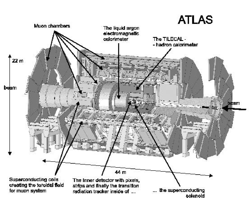
Figure 79: The overall layout of the ATLAS detector.

The ATLAS muon spectrometer is located behind the calorimeters, thus shielded from hadronic showers. The spectrometer uses several tracking technologies along with a toroidal magnet, providing a 4 T field for an independent momentum measurement outside the calorimeter volume. Most of the spectrometer volume is covered by Monitored Drift Tubes (MDT). In the forward region, where the rate is high, Cathode Strip Chambers are used. The standalone muon spectrometer momentum resolution is of the order of $2\%$ for muons with $10\leq p_{T}\leq 100$ GeV. The muon spectrometer covers $\mid\eta\mid<2.7$.

The ATLAS trigger and data acquisition system is multi-level and has to reduce the beam crossing rate of 40 MHz to an output to mass storage rate of $\mathcal{O}(100)$ Hz. The first stage (LVL1) is a hardware-based trigger, making use of the coarse granularity calorimeter data and the dedicated muon trigger chambers only, reducing the output rate to about 75 kHz, within a maximum latency of 2.5 $\mu$s.

The performance results have been obtained using a detailed full simulation of the ATLAS detector response with GEANT and have been validated by an extensive program of test beam measurements of all components.

10.2 Heavy Flavour studies in ATLAS

Recent theoretical investigations [147] have indicated that a dense partonic medium will suppress the gluon radiation from charm and bottom quarks relative to that from light quarks. Thus $b$-jet measurements in ATLAS would provide an important comparison measurement to light quark and gluon jets. Such measurements would have important implications for gluon shadowing and saturation effects. Tagging of $b$-jets by the associated muon is possible in the $pp$ environment [265].

It is unlikely that vertexing will be available for these studies due to the high multiplicity Pb+Pb environment. Therefore we are currently studying the possibility of tagging $b$-jets by matching a measured muon in the muon spectrometer to the jet measured by the calorimeter. Vertexing will be available for lighter ion and $pA$ collisions.

We will profit from current studies of ATLAS performance for soft lepton tagging of the $H\rightarrow b\bar{b}$ decay. Initial studies of the detector performance for $b$-jet tagging using this technique can be found in the TDR for high luminosity $pp$ collisions [266]. We note that the muon momentum should be larger than 4 GeV to be detected in the spectrometer. The expected muon background comes from $\pi$, $K$ and $c$ decays.

Quarkonia suppression is expected in a deconfined medium due to the screening of the long-range attractive potential. We are beginning studies of the ATLAS capability for $\Upsilon$ identification. The initial evaluation is that the muon system alone will provide marginal resolution for a clear separation of the three states. However, use of the SCT and pixel detectors can enhance the mass resolution. Initial full simulations of Pb+Pb collisions indicate that the occupancies in the Inner Detector (with the exception of the Transition Radiation Tracker) are low enough to allow track reconstruction. We expect that all of the inner detectors will be available for lighter ion and $pA$ collisions. The expected occupancies obtained from preliminary full detector simulations using HIJING are listed in Table 35 for the barrel detectors in the Inner Detector. In the endcaps, the Inner Detector covers $1.4\leq\eta\leq 2.5$ with average occupancies of 0.2% for the silicon pixels and 6% and 10% for the SCT, depending on the SCT wheel. There are 9 SCT tracking stations on each endcap which should allow tracking in the forward direction as well.

Table 35: Segmentation and occupancies of the Inner Detector (Barrel). Values were obtained from preliminary full detector simulations using HIJING with $dN_{\rm ch}/d\eta=8000$. The $pp$ occupancies are from Ref. [267]. The corresponding $pp$ and Pb+Pb luminosities are also quoted.

ID	$\eta$ range	Radius (cm)	Channels	Occupancy	Occupancy
				$pp$ ($10^{34})$	Pb+Pb ($10^{27}$)
Si Pixel 1	$\pm 2.5$	5.0	$10^{7}$	0.04	0.6
Si Pixel 2	$\pm 1.7$	8.8	$8\times 10^{7}$	0.01	0.3
Si Pixel 3	$\pm 1.7$	12.2	$8\times 10^{7}$	0.006	0.2
SCT Layer 1	$\pm 1.4$	30.0	$3\times 10^{6}$	0.6	15
SCT Layer 1	$\pm 1.4$	37.0	$3\times 10^{6}$	0.5	10
SCT Layer 1	$\pm 1.4$	44.0	$3\times 10^{6}$	0.4	7.5
SCT Layer 1	$\pm 1.4$	51.5	$3\times 10^{6}$	0.3	6.0

The muon spectrometer will benefit from the low nucleus-nucleus luminosity. In the high luminosity $pp$ runs a large number of spectrometer hits come from slow neutrons produced in previous interactions. Initial simulations using HIJING Pb+Pb events indicate that the muon spectrometer is sparsely populated. The muon backgrounds are from $\pi$ and $K$ decays in the calorimeter. However, a substantial number of these decays are expected to be rejected when matches to Inner Detector tracks are required. The minimum muon $p_{T}$ for detection is $\sim 5-6$ GeV.

Acknowledgments The authors would like to thank their collaborators in ATLAS: S. Aronson, K. Assamagan, M. Dobbs, J. Dolesji, H. Gordon, F. Gianotti, S. Kabana, M. Levine, F. Marroquim, J. Nagle, P. Nevski, A. Olszewski, L. Rosselet, P. Sawicki, A. Trzupek, M. A. B. Vale, S. White, R. Witt, B. Wosiek and K. Wozniak.

11 ACKNOWLEDGEMENTS

The following sources of funding are acknowledged:

Academy of Finland,

Grant 102046: P. Hoyer;

2002 CNRS/SNF Cooperation Program,

Grant 11240: N. Marchal, S. Peigné;

European Commission IHP program,

Contract HPRN-CT-2000-00130;

DFG Grant No. 436 RUS 17/129/02: D. Blaschke;

United States Department of Energy, Division of Nuclear Physics,

Contract No. DE-AC02-98CH10886: D. Kharzeev, P. Petreczky;

Grant No. DE-FG03-95ER40937: R.L. Thews;

Contract No. DE-AC03-76SF00098: R. Vogt;

United States Department of Energy, Division of High Energy Physics,

Contract No. W-31-109-ENG-38: G.T. Bodwin, Jungil Lee.

References

- [1] T. Matsui and H. Satz, Phys. Lett. B 178 (1986) 416.
- [2] P. Nason, S. Dawson and R. K. Ellis, Nucl. Phys. B 303 (1988) 607.
- [3] P. Nason, S. Dawson and R. K. Ellis, Nucl. Phys. B 327 (1989) 49 [Erratum-ibid. B 335 (1990) 260].
- [4] W. Beenakker, W. L. van Neerven, R. Meng, G. A. Schuler and J. Smith, Nucl. Phys. B 351 (1991) 507.
- [5] M. L. Mangano, P. Nason and G. Ridolfi, Nucl. Phys. B 373 (1992) 295.
- [6] S. Frixione, M. L. Mangano, P. Nason and G. Ridolfi, Nucl. Phys. B 431 (1994) 453.
- [7] S. Frixione, M. L. Mangano, P. Nason and G. Ridolfi, Adv. Ser. Direct. High Energy Phys. 15 (1998) 609 [arXiv:hep-ph/9702287].
- [8] M. Cacciari and P. Nason, Phys. Rev. Lett. 89 (2002) 122003 [arXiv:hep-ph/0204025].
- [9] M. Cacciari and P. Nason, JHEP 0309 (2003) 006 [arXiv:hep-ph/0306212].
- [10] S. Frixione, P. Nason and B. R. Webber, JHEP 0308 (2003) 007 [arXiv:hep-ph/0305252].
- [11] D. Acosta [CDF Collaboration], arXiv:hep-ex/0307080.
- [12] A. Korn [CDF Collaboration], arXiv:hep-ex/0305054.
- [13] A. D. Martin, R. G. Roberts, W. J. Stirling and R. S. Thorne, Eur. Phys. J. C 14 (2000) 133 [arXiv:hep-ph/9907231].
- [14] A. D. Martin, R. G. Roberts, W. J. Stirling and R. S. Thorne, Eur. Phys. J. C 23 (2002) 73 [arXiv:hep-ph/0110215].
- [15] J. Pumplin, D. R. Stump, J. Huston, H. L. Lai, P. Nadolsky and W. K. Tung, JHEP 0207 (2002) 012 [arXiv:hep-ph/0201195].
- [16] K. J. Eskola, V. J. Kolhinen and P. V. Ruuskanen, Nucl. Phys. B 535 (1998) 351 [arXiv:hep-ph/9802350].
- [17] K. J. Eskola, V. J. Kolhinen and C. A. Salgado, Eur. Phys. J. C 9 (1999) 61 [arXiv:hep-ph/9807297].
- [18] V. D. Barger, W. Y. Keung and R. J. Phillips, Phys. Lett. B 91 (1980) 253.
- [19] V. D. Barger, W. Y. Keung and R. J. Phillips, Z. Phys. C 6 (1980) 169.
- [20] R. Gavai, D. Kharzeev, H. Satz, G. A. Schuler, K. Sridhar and R. Vogt, Int. J. Mod. Phys. A 10 (1995) 3043 [arXiv:hep-ph/9502270].
- [21] G. A. Schuler and R. Vogt, Phys. Lett. B 387 (1996) 181 [arXiv:hep-ph/9606410].
- [22] R. Vogt, Prepared for 18th Winter Workshop on Nuclear Dynamics, Nassau, The Bahamas, 20-27 Jan 2002, EP Systema, Debrecen, Hungary, p.253 [arXiv:hep-ph/0203151].
- [23] R. Vogt, Prepared for Budapest 2002 Workshop on Quark and Hadron Dynamics, Budapest, Hungary, 3-7 March 2002, EP Systema, Debrecen, Hungary, p. 223 [arXiv:hep-ph/0205330].
- [24] A. D. Martin, R. G. Roberts, W. J. Stirling and R. S. Thorne, Eur. Phys. J. C 4 (1998) 463 [arXiv:hep-ph/9803445].
- [25] H. L. Lai et al. [CTEQ Collaboration], Eur. Phys. J. C 12 (2000) 375 [arXiv:hep-ph/9903282].
- [26] M. Gluck, E. Reya and A. Vogt, Eur. Phys. J. C 5 (1998) 461 [arXiv:hep-ph/9806404].
- [27] S. Digal, P. Petreczky and H. Satz, Phys. Rev. D 64 (2001) 094015 [arXiv:hep-ph/0106017].
- [28] T. Affolder et al. [CDF Collaboration], Phys. Rev. Lett. 84 (2000) 2094 [arXiv:hep-ex/9910025].
- [29] J. F. Gunion and R. Vogt, Nucl. Phys. B 492 (1997) 301 [arXiv:hep-ph/9610420].
- [30] A. D. Martin, W. J. Stirling and R. G. Roberts, Phys. Lett. B 306 (1993) 145 [Erratum-ibid. B 309 (1993) 492].
- [31] M. Gluck, E. Reya and A. Vogt, Z. Phys. C 53 (1992) 127.
- [32] W. E. Caswell and G. P. Lepage, Phys. Lett. B 167 (1986) 437.
- [33] B. A. Thacker and G. P. Lepage, Phys. Rev. D 43 (1991) 196.
- [34] G. T. Bodwin, E. Braaten and G. P. Lepage, Phys. Rev. D 51 (1995) 1125; 55 (1997) 5853(E) [arXiv:hep-ph/9407339].
- [35] See G. A. Schuler, arXiv:hep-ph/9403387, and references therein.
- [36] G. T. Bodwin, S. Kim and D. K. Sinclair, Nucl. Phys. B (Proc. Suppl.) 34 (1994) 434.
- [37] G. T. Bodwin, D. K. Sinclair and S. Kim, Phys. Rev. D 65 (2002) 054504 [arXiv:hep-lat/0107011].
- [38] J. w. Qiu and G. Sterman (private communication).
- [39] F. Abe et al. [CDF Collaboration], Phys. Rev. Lett. 79 (1997) 572.
- [40] M. Kramer, Prog. Part. Nucl. Phys. 47 (2001) 141 [arXiv:hep-ph/0106120].
- [41] E. Braaten, S. Fleming and A. K. Leibovich, Phys. Rev. D 63 (2001) 094006 [arXiv:hep-ph/0008091].
- [42] P. L. Cho and M. B. Wise, Phys. Lett. B 346 (1995) 129 [arXiv:hep-ph/9411303].
- [43] M. Beneke and I. Z. Rothstein, Phys. Lett. B 372 (1996) 157 [Erratum-ibid. B 389 (1996) 769] [arXiv:hep-ph/9509375].
- [44] A. K. Leibovich, Phys. Rev. D 56 (1997) 4412 [arXiv:hep-ph/9610381].
- [45] M. Beneke and M. Kramer, Phys. Rev. D 55 (1997) 5269 [arXiv:hep-ph/9611218].
- [46] E. Braaten, B. A. Kniehl, and J. Lee, Phys. Rev. D 62 (2000) 094005 [arXiv:hep-ph/9911436].
- [47] B. A. Kniehl and J. Lee, Phys. Rev. D 62, 114027 (2000) [arXiv:hep-ph/0007292].
- [48] T. Affolder et al. [CDF Collaboration], Phys. Rev. Lett. 85 (2000) 2886 [arXiv:hep-ex/0004027].
- [49] G. T. Bodwin and J. Lee, arXiv:hep-ph/0308016.
- [50] D. Acosta et al. [CDF Collaboration], Phys. Rev. Lett. 88 (2002) 161802.
- [51] E. Braaten and J. Lee, Phys. Rev. D 63 (2001) 071501 [arXiv:hep-ph/0012244].
- [52] M. Klasen, B. A. Kniehl, L. N. Mihaila and M. Steinhauser, Phys. Rev. Lett. 89 (2002) 032001 [arXiv:hep-ph/0112259].
- [53] P. L. Cho, Phys. Lett. B 368 (1996) 171 [arXiv:hep-ph/9509355].
- [54] S. Todorova-Nova, in Proceedings of the XXXI International Symposium on Multiparticle Dynamics, Datong, China, 1–7 September, 2001 (World Scientific, Singapore, to appear) arXiv:hep-ph/0112050.
- [55] M. Chapkine, talk presented at 7th International Workshop on Meson Production, Properties and Interaction (Meson 2002), Krakow, Poland, May 24–28, 2002; unpublished.
- [56] G. Alexander et al. [OPAL Collaboration], Phys. Lett. B 370 (1996) 185.
- [57] K. Abe et al. [BELLE Collaboration], Phys. Rev. Lett. 88 (2002) 052001 [arXiv:hep-ex/0110012].
- [58] B. Aubert et al. [BABAR Collaboration], Phys. Rev. Lett. 87 (2001) 162002 [arXiv:hep-ex/0106044].
- [59] K. Abe et al. [Belle Collaboration], Phys. Rev. Lett. 89 (2002) 142001 [arXiv:hep-ex/0205104].
- [60] P. L. Cho and A. K. Leibovich, Phys. Rev. D 54 (1996) 6690 [arXiv:hep-ph/9606229].
- [61] P. Merkel, Nucl. Phys. Proc. Suppl. 79 (1999) 371.
- [62] A. Bertolin [ZEUS and H1 Collaborations], Prepared for 30th International Conference on High-Energy Physics (ICHEP 2000), Osaka, Japan, 27 Jul - 2 Aug 2000
- [63] A. Meyer, DESY-THESIS-1998-012; A. Meyer (unpublished).
- [64] S. Mohrdieck, DESY-THESIS-2000-059.
- [65] G. T. Bodwin, S. J. Brodsky and G. P. Lepage, Phys. Rev. D 39 (1989) 3287.
- [66] J. w. Qiu and G. Sterman, Int. J. Mod. Phys. E 12 (2003) 149 [arXiv:hep-ph/0111002].
- [67] G. T. Bodwin, S. J. Brodsky and G. P. Lepage, Phys. Rev. Lett. 47 (1981) 1799.
- [68] G. T. Bodwin, Phys. Rev. D 31 (1985) 2616; D 34 (1986) 3932(E)].
- [69] M. Beneke and I. Z. Rothstein, Phys. Rev. D 54 (1996) 2005 [Erratum-ibid. D 54 (1996) 7082] [arXiv:hep-ph/9603400].
- [70] P. L. Cho and A. K. Leibovich, Phys. Rev. D 53 (1996) 150 [arXiv:hep-ph/9505329].
- [71] P. L. Cho and A. K. Leibovich, Phys. Rev. D 53 (1996) 6203 [arXiv:hep-ph/9511315].
- [72] E. Braaten and T. C. Yuan, Phys. Rev. Lett. 71 (1993) 1673 [arXiv:hep-ph/9303205].
- [73] E. Braaten and S. Fleming, Phys. Rev. Lett. 74 (1995) 3327 [arXiv:hep-ph/9411365].
- [74] M. Cacciari, M. Greco, M. L. Mangano and A. Petrelli, Phys. Lett. B 356 (1995) 553 [arXiv:hep-ph/9505379].
- [75] B. A. Kniehl and G. Kramer, Eur. Phys. J. C 6 (1999) 493 [arXiv:hep-ph/9803256].
- [76] B. A. Kniehl and G. Kramer, Phys. Rev. D 60 (1999) 014006 [arXiv:hep-ph/9901348].
- [77] F. Abe et al. [CDF Collaboration], Phys. Rev. Lett. 79 (1997) 578.
- [78] A. D. Martin, R. G. Roberts, W. J. Stirling and R. S. Thorne, Phys. Lett. B 443 (1998) 301 [arXiv:hep-ph/9808371].
- [79] E. L. Berger and D. L. Jones, Phys. Rev. D 23 (1981) 1521.
- [80] R. Baier and R. Ruckl, Phys. Lett. B 102 (1981) 364.
- [81] C. Adloff et al. [H1 Collaboration], Eur. Phys. J. C 25 (2002) 25 [arXiv:hep-ex/0205064].
- [82] C. Adloff et al. [H1 Collaboration], Eur. Phys. J. C 25 (2002) 41 [arXiv:hep-ex/0205065].
- [83] D. M. Kaplan [E789 Collaboration], Int. J. Mod. Phys. A 12 (1997) 3827 [arXiv:hep-ex/9610003].
- [84] F. Abe et al. [CDF Collaboration], Phys. Rev. Lett. 75 (1995) 4358.
- [85] T. Alexopoulos et al. [E771 Collaboration], Phys. Lett. B 374 (1996) 271.
- [86] A. Bertolin [H1 and ZEUS Collaborations], Prepared for International Europhysics Conference on High-Energy Physics (EPS-HEP 99), Tampere, Finland, 15-21 Jul 1999. Published in ‘Tampere 1999, High energy physics’ 580-582.
- [87] T. Alexopoulos et al. [E-771 Collaboration], Phys. Rev. D 55 (1997) 3927.
- [88] C. Lourenco, Nucl. Phys. A 610 (1996) 552C [arXiv:hep-ph/9612222].
- [89] M. Vänttinen, P. Hoyer, S. J. Brodsky and W. K. Tang, Phys. Rev. D 51 (1995) 3332 [arXiv:hep-ph/9410237].
- [90] P. Roudeau [NA14 Collaboration], Nucl. Phys. Proc. Suppl. 7B (1989) 273.
- [91] L. Antoniazzi et al. [E705 Collaboration], Phys. Rev. Lett. 70 (1993) 383.
- [92] L. Antoniazzi et al. [E705 Collaboration], Phys. Rev. D 49 (1994) 543.
- [93] P. Hoyer and S. Peigné, Phys. Rev. D 59 (1999) 034011 [arXiv:hep-ph/9806424].
- [94] P. Hoyer, Nucl. Phys. Proc. Suppl. 75B (1999) 153 [arXiv:hep-ph/9809362].
- [95] E. M. Aitala et al. [E791 Collaboration], Eur. Phys. J. C 4 (1999) 1 [arXiv:hep-ex/9809029].
- [96] P. L. Frabetti et al. [E687 Collaboration], Phys. Lett. B 370 (1996) 222.
- [97] N. Marchal, S. Peigné and P. Hoyer, Phys. Rev. D 62 (2000) 114001 [arXiv:hep-ph/0004234].
- [98] H. Fritzsch, Phys. Lett. B 67 (1977) 217.
- [99] F. Halzen, Phys. Lett. B 69 (1977) 105.
- [100] M. Gluck, J. F. Owens and E. Reya, Phys. Rev. D 17 (1978) 2324.
- [101] P. Hoyer and S. Peigné, Phys. Rev. D 61 (2000) 031501.
- [102] V. Koreshev et al. [E672-E706 Collaborations], Phys. Rev. Lett. 77 (1996) 4294.
- [103] T. Alexopoulos et al. [E771 Collaboration], Phys. Rev. D 62 (2000) 032006 [arXiv:hep-ex/9908010].
- [104] P. Hoyer, M. Vänttinen and U. Sukhatme, Phys. Lett. B 246 (1990) 217.
- [105] M. J. Leitch et al. [FNAL E866/NuSea collaboration], Phys. Rev. Lett. 84 (2000) 3256 [arXiv:nucl-ex/9909007].
- [106] P. Amaudruz et al. [New Muon Collaboration], Nucl. Phys. B 371 (1992) 553.
- [107] D. M. Alde et al., Phys. Rev. Lett. 66 (1991) 2285.
- [108] M. J. Leitch et al. [E772 and E789 Collaboration], Nucl. Phys. A 544 (1992) 197C.
- [109] M. C. Abreu et al., Phys. Lett. B 466 (1999) 408.
- [110] C. Baglin et al. [NA38 Collaboration], Phys. Lett. B 220 (1989) 471.
- [111] C. Baglin et al. [NA38 Collaboration], Phys. Lett. B 251 (1990) 465.
- [112] C. Baglin et al. [NA38 Collaboration], Phys. Lett. B 255 (1991) 459.
- [113] A. Capella, J. A. Casado, C. Pajares, A. V. Ramallo and J. Tran Thanh Van, Phys. Lett. B 206 (1988) 354.
- [114] C. Gerschel and J. Hufner, Z. Phys. C 56 (1992) 171.
- [115] D. Kharzeev, C. Lourenço, M. Nardi and H. Satz, Z. Phys. C 74 (1997) 307 [arXiv:hep-ph/9612217].
- [116] M. C. Abreu et al., arXiv:hep-ex/0207014.
- [117] M. C. Abreu et al. [NA38/NA50 Collaboration], Nucl. Phys. A 698 (2002) 539.
- [118] M. Leitch, in proceedings of International Workshop on the Physics of the Quark Gluon Plasma, Palaiseau, Sept. 2001. For transparencies, see the home page, http://polywww.in2p3.fr/CIPPQG.
- [119] A. Deandrea, G. Nardulli and A.D. Polosa, in preparation.
- [120] Z.W. Lin and C.M. Ko, Phys. Rev. C 62 (2000) 034903 [arXiv:nucl-th/9912046].
- [121] K. L. Haglin and C. Gale, Phys. Rev. C 63 (2001) 065201 [arXiv:nucl-th/0010017].
- [122] Y. Oh, T. Song and S.H. Lee, Phys. Rev. C 63 (2001) 034901 [arXiv:nucl-th/0010064].
- [123] J. w. Qiu, J. P. Vary and X. f. Zhang, Phys. Rev. Lett. 88 (2002) 232301 [arXiv:hep-ph/9809442].
- [124] P. Colangelo, F. De Fazio and G. Nardulli, Phys. Lett. B 334 (1994) 175 [arXiv:hep-ph/9406320].
- [125] P. Colangelo, G. Nardulli, A. Deandrea, N. Di Bartolomeo, R. Gatto and F. Feruglio, Phys. Lett. B 339 (1994) 151 [arXiv:hep-ph/9406295].
- [126] R. Casalbuoni, A. Deandrea, N. Di Bartolomeo, R. Gatto, F. Feruglio and G. Nardulli, Phys. Rept. 281 (1997) 145 [arXiv:hep-ph/9605342].
- [127] S. Ahmed et al. [CLEO Collaboration], Phys. Rev. Lett. 87 (2001) 251801 [arXiv:hep-ex/0108013].
- [128] R. D. Matheus, F. S. Navarra, M. Nielsen and R. Rodrigues da Silva, Phys. Lett. B 541 (2002) 265 [arXiv:hep-ph/0206198].
- [129] F. O. Duraes, S. H. Lee, F. S. Navarra and M. Nielsen, Phys. Lett. B 564 (2003) 97 [arXiv:nucl-th/0210075].
- [130] A. Deandrea, N. Di Bartolomeo, R. Gatto, G. Nardulli and A.D. Polosa, Phys. Rev. D 58 (1998) 034004 [arXiv:hep-ph/9802308].
- [131] A.D. Polosa, Riv. Nuovo Cim. 23N11 (2000) 1 [arXiv:hep-ph/0004183].
- [132] M. Ademollo and R. Gatto, Phys. Rev. Lett. 13 (1964) 264.
- [133] M. E. Luke, Phys. Lett. B 252 (1990) 447.
- [134] A. F. Falk, H. Georgi, B. Grinstein and M. B. Wise, Nucl. Phys. B 343 (1990) 1.
- [135] E. Shuryak, Phys. Rev. C 55 (1997) 961 [arXiv:nucl-th/9605011].
- [136] Z. w. Lin, R. Vogt and X. N. Wang, Phys. Rev. C 57 (1998) 899 [arXiv:nucl-th/9705006].
- [137] Z. w. Lin and R. Vogt, Nucl. Phys. B 544 (1999) 339 [arXiv:hep-ph/9808214].
- [138] M. G. Mustafa, D. Pal, D. K. Srivastava and M. Thoma, Phys. Lett. B 428 (1998) 234 [arXiv:nucl-th/9711059].
- [139] D. K. Srivastava, C. Gale and T. C. Awes, arXiv:nucl-th/0212081.
- [140] E. Braaten and M. H. Thoma, Phys. Rev. D 44 (1991) 2625.
- [141] M. H. Thoma and M. Gyulassy, Nucl. Phys. B 351 (1991) 491.
- [142] R. Baier, M. Dirks and K. Redlich, arXiv:hep-ph/9910353.
- [143] J. P. Blaizot and E. Iancu, Phys. Rept. 359 (2002) 355 [arXiv:hep-ph/0101103].
- [144] M. Gyulassy and X. n. Wang, Nucl. Phys. B 420 (1994) 583 [arXiv:nucl-th/9306003].
- [145] R. Baier, Y. L. Dokshitzer, S. Peigne and D. Schiff, Phys. Lett. B 345 (1995) 277 [arXiv:hep-ph/9411409].
- [146] B. G. Zakharov, JETP Lett. 63 (1996) 952 [arXiv:hep-ph/9607440].
- [147] Yu. L. Dokshitzer and D. E. Kharzeev, Phys. Lett. B 519 (2001) 199 [arXiv:hep-ph/0106202].
- [148] K. Adcox et al. [PHENIX Collaboration], Phys. Rev. Lett. 88 (2002) 192303 [arXiv:nucl-ex/0202002].
- [149] R. Averbeck [PHENIX Collaboration], Nucl. Phys. A 715 (2003) 695 [arXiv:nucl-ex/0209016].
- [150] K. Gallmeister, B. Kampfer and O. P. Pavlenko, Nucl. Phys. A 715 (2003) 705 [arXiv:nucl-th/0208006].
- [151] S. Batsouli, S. Kelly, M. Gyulassy and J. L. Nagle, Phys. Lett. B 557 (2003) 26 [arXiv:nucl-th/0212068].
- [152] I. P. Lokhtin, arXiv:hep-ph/0210010.
- [153] R. Baier, Y. L. Dokshitzer, A. H. Mueller, S. Peigne and D. Schiff, Nucl. Phys. B 484 (1997) 265 [arXiv:hep-ph/9608322].
- [154] Y. L. Dokshitzer, V. A. Khoze and S. I. Troian, Phys. Rev. D 53 (1996) 89 [arXiv:hep-ph/9506425].
- [155] P. Nason and B. R. Webber, Phys. Lett. B 395 (1997) 355 [arXiv:hep-ph/9612353].
- [156] B. A. Schumm, Y. L. Dokshitzer, V. A. Khoze and D. S. Koetke, Phys. Rev. Lett. 69 (1992) 3025.
- [157] Y. L. Dokshitzer, V. A. Khoze and S. I. Troian, J. Phys. G 17 (1991) 1481.
- [158] R. Baier, Y. L. Dokshitzer, A. H. Mueller and D. Schiff, JHEP 0109 (2001) 033 [arXiv:hep-ph/0106347].
- [159] P. L. McGaughey, E. Quack, P. V. Ruuskanen, R. Vogt and X. N. Wang, Int. J. Mod. Phys. A 10 (1995) 2999 [arXiv:hep-ph/9411438].
- [160] A. Bazilevsky [PHENIX Collaboration], Nucl. Phys. A 715 (2003) 486 [arXiv:nucl-ex/0209025].
- [161] R. L. Thews, Nucl. Phys. A 702 (2002) 341 [arXiv:hep-ph/0111015].
- [162] P. Braun-Munzinger, D. Magestro, K. Redlich and J. Stachel, Phys. Lett. B 518 (2001) 41 [arXiv:hep-ph/0105229].
- [163] P. Braun-Munzinger and J. Stachel, Phys. Lett. B 490 (2000) 196 [arXiv:nucl-th/0007059].
- [164] A. Andronic, P. Braun-Munzinger, K. Redlich and J. Stachel, Nucl. Phys. A 715 (2003) 529 [arXiv:nucl-th/0209035].
- [165] D. Kharzeev, E. Levin and M. Nardi, arXiv:hep-ph/0111315.
- [166] M. I. Gorenstein, A. P. Kostyuk, H. Stocker and W. Greiner, Phys. Lett. B 509 (2001) 277 [arXiv:hep-ph/0010148].
- [167] J. Cleymans, K. Redlich and E. Suhonen, Z. Phys. C 51 (1991) 137.
- [168] M. I. Gorenstein, A. P. Kostyuk, H. Stocker and W. Greiner, Phys. Lett. B 524 (2002) 265 [arXiv:hep-ph/0104071].
- [169] L. Grandchamp and R. Rapp, Nucl. Phys. A 715 (2003) 545 [arXiv:hep-ph/0209141].
- [170] L. Grandchamp and R. Rapp, Nucl. Phys. A 709 (2002) 415 [arXiv:hep-ph/0205305].
- [171] L. Grandchamp and R. Rapp, Phys. Lett. B 523 (2001) 60 [arXiv:hep-ph/0103124].
- [172] H. Sorge, E. V. Shuryak and I. Zahed, Phys. Rev. Lett. 79 (1997) 2775 [arXiv:hep-ph/9705329].
- [173] R. L. Thews, M. Schroedter and J. Rafelski, Phys. Rev. C 63 (2001) 054905 [arXiv:hep-ph/0007323].
- [174] R. L. Thews and J. Rafelski, Nucl. Phys. A 698 (2002) 575 [arXiv:hep-ph/0104025].
- [175] D. Kharzeev and H. Satz, Phys. Lett. B 334 (1994) 155 [arXiv:hep-ph/9405414].
- [176] R. L. Thews, Published in the proceedings of Pan American Advanced Studies Institute: New States of Matter in Hadronic Interactions (PASI 2002), Campos do Jordao 2002, 490 [arXiv:hep-ph/0206179].
- [177] R. Vogt [Hard Probe Collaboration], Int. J. Mod. Phys. E 12 (2003) 211 [arXiv:hep-ph/0111271].
- [178] M. L. Mangano and R. L. Thews, in progress.
- [179] K. Adcox et al. [PHENIX Collaboration], Phys. Rev. Lett. 88 (2002) 192302 [arXiv:nucl-ex/0201008].
- [180] A. D. Frawley [PHENIX Collaboration], Nucl. Phys. A 715 (2003) 687 [arXiv:nucl-ex/0210013].
- [181] K. Redlich and A. Tounsi, Eur. Phys. J. C 24 (2002) 589 [arXiv:hep-ph/0111261].
- [182] B. Zhang, C. M. Ko, B. A. Li, Z. W. Lin and S. Pal, Phys. Rev. C 65 (2002) 054909 [arXiv:nucl-th/0201038].
- [183] D. Kharzeev and H. Satz, arXiv:hep-ph/9505345.
- [184] X. M. Xu, D. Kharzeev, H. Satz and X. N. Wang, Phys. Rev. C 53 (1996) 3051 [arXiv:hep-ph/9511331].
- [185] E. V. Shuryak, Phys. Lett. B 78 (1978) 150 [Sov. J. Nucl. Phys. 28 (1978 YAFIA,28,796-808.1978) 408.1978 YAFIA,28,796].
- [186] G. Bhanot and M. E. Peskin, Nucl. Phys. B 156 (1979) 391.
- [187] D. Kharzeev, L. D. McLerran and H. Satz, Phys. Lett. B 356 (1995) 349 [arXiv:hep-ph/9504338].
- [188] C. Y. Wong, Phys. Rev. C 65 (2002) 034902 [arXiv:nucl-th/0110004].
- [189] D. Kharzeev, Nucl. Phys. A 610 (1996) 418C [arXiv:hep-ph/9609260].
- [190] G. Röpke, D. Blaschke and H. Schulz, Phys. Rev. D 38 (1988) 3589.
- [191] G.W. Fehrenbach, W. Schäfer, J. Treusch, R.G. Ulbrich, Phys. Rev. Lett. 49 (1982) 1281.
- [192] F. Karsch, M. T. Mehr and H. Satz, Z. Phys. C 37 (1988) 617.
- [193] T. Hashimoto, K. Hirose, T. Kanki and O. Miyamura, Z. Phys. C 38 (1988) 251.
- [194] T. Umeda, K. Nomura and H. Matsufuru, arXiv:hep-lat/0211003.
- [195] S. Datta, F. Karsch, P. Petreczky and I. Wetzorke, arXiv:hep-lat/0208012.
- [196] S. Digal, S. Fortunato, P. Petreczky and H. Satz, Phys. Lett. B 549 (2002) 101 [arXiv:hep-ph/0207264].
- [197] Y. Nakahara, M. Asakawa and T. Hatsuda, Phys. Rev. D 60 (1999) 091503 [arXiv:hep-lat/9905034].
- [198] M. Asakawa, T. Hatsuda and Y. Nakahara, Prog. Part. Nucl. Phys. 46 (2001) 459 [arXiv:hep-lat/0011040].
- [199] F. Karsch, S. Datta, E. Laermann, P. Petreczky, S. Stickan and I. Wetzorke, Nucl. Phys. A 715 (2003) 701 [arXiv:hep-ph/0209028].
- [200] M. Asakawa, T. Hatsuda and Y. Nakahara, Nucl. Phys. A 715 (2003) 863 [arXiv:hep-lat/0208059].
- [201] T. Umeda, R. Katayama, O. Miyamura and H. Matsufuru, Int. J. Mod. Phys. A 16 (2001) 2215 [arXiv:hep-lat/0011085].
- [202] M. Luscher, S. Sint, R. Sommer and H. Wittig, Nucl. Phys. B 491 (1997) 344 [arXiv:hep-lat/9611015].
- [203] O. Philipsen, arXiv:hep-ph/0010327.
- [204] O. Philipsen, Phys. Lett. B 535 (2002) 138 [arXiv:hep-lat/0203018].
- [205] O. Kaczmarek, F. Karsch, P. Petreczky and F. Zantow, Phys. Lett. B 543 (2002) 41 [arXiv:hep-lat/0207002].
- [206] F. Arleo, P. B. Gossiaux, T. Gousset and J. Aichelin, Phys. Rev. D 65 (2002) 014005 [arXiv:hep-ph/0102095].
- [207] D. Kharzeev, arXiv:nucl-th/9601029.
- [208] J. D. Bjorken, Phys. Rev. D 27 (1983) 140.
- [209] G. Röpke, D. Blaschke and H. Schulz, Phys. Lett. B 202 (1988) 479.
- [210] T. Sjöstrand, P. Edén, C. Friberg, L. Lönnblad, G. Miu, S. Mrenna and E. Norrbin, Comput. Phys. Commun. 135 (2001) 238 [arXiv:hep-ph/0010017].
- [211] T. Sjöstrand, Comput. Phys. Commun. 82 (1994) 74.
- [212] G. Corcella et al., JHEP 0101 (2001) 010 [arXiv:hep-ph/0011363].
- [213] G. Corcella et al., arXiv:hep-ph/0201201.
- [214] G. Marchesini, B. R. Webber, G. Abbiendi, I. G. Knowles, M. H. Seymour and L. Stanco, Comput. Phys. Commun. 67 (1992) 465.
- [215] X. N. Wang and M. Gyulassy, Phys. Rev. D 44 (1991) 3501.
- [216] M. Gyulassy and X. N. Wang, Comput. Phys. Commun. 83 (1994) 307 [arXiv:nucl-th/9502021].
- [217] E. Norrbin and T. Sjöstrand, Eur. Phys. J. C 17 (2000) 137 [arXiv:hep-ph/0005110].
- [218] B.R. Webber, private communication.
- [219] B. Andersson, G. Gustafson and B. Nilsson-Almqvist, Nucl. Phys. B 281 (1987) 289.
- [220] A. Capella, U. Sukhatme, C. I. Tan and J. Tran Thanh Van, Phys. Rept. 236 (1994) 225.
- [221] K. J. Eskola, P. V. Ruuskanen, S. S. Räsänen and K. Tuominen, Nucl. Phys. A 696 (2001) 715 [arXiv:hep-ph/0104010].
- [222] S. Frixione and B. R. Webber, JHEP 0206 (2002) 029 [arXiv:hep-ph/0204244].
- [223] [ALICE Collaboration], CERN-LHCC-95-71.
- [224] [ALICE Collaboration], ALICE Physics Performance Report, in preparation; ALICE-INT-2002-25.
- [225] M. C. Abreu et al. [NA50 Collaboration], Phys. Lett. B 477 (2000) 28.
- [226] H. Satz, Rept. Prog. Phys. 63 (2000) 1511 [arXiv:hep-ph/0007069].
- [227] R. Vogt, Phys. Rept. 310 (1999) 197.
- [228] D. E. Groom et al. [Particle Data Group Collaboration], Eur. Phys. J. C 15 (2000) 1.
- [229] P. Braun-Munzinger and K. Redlich, Eur. Phys. J. C 16 (2000) 519 [arXiv:hep-ph/0001008].
- [230] B. Müller and X. N. Wang, Phys. Rev. Lett. 68 (1992) 2437.
- [231] K. Geiger, Phys. Rev. D 48 (1993) 4129.
- [232] M.C. Abreu et al. [NA50 collaboration], Eur. Phys. J. C 14 (2000) 443.
- [233] S. Beole et al. [ALICE Collaboration], CERN-LHCC-96-32.
- [234] A. Morsch [ALICE Collaboration], Nucl. Phys. A 638 (1998) 571.
- [235] A. Morsch, R. Raniwala, S. Raniwala and Y. Viyogi, [ALICE Collaboration], ALICE-INT-2001-22.
- [236] A. Morsch, private communication.
- [237] P. Crochet and P. Braun-Munzinger, Nucl. Instrum. Meth. A 484 (2002) 564 [arXiv:nucl-ex/0106008].
- [238] [ALICE Collaboration], CERN-LHCC-2001-021.
- [239] M. Lunardon and R. Turrisi, [ALICE Collaboration], to be submitted.
- [240] [ALICE Collaboration], CERN-LHCC-99-13.
- [241] A. Chilingarov et al., Phys. Lett. B 83 (1979) 136.
- [242] T. Akesson et al., Z. Phys. C 72 (1996) 429.
- [243] [PHENIX Collaboration], Conceptual Design Report, BNL 48922 (1993).
- [244] [ALICE Collaboration], CERN-LHCC-99-22.
- [245] [ALICE Collaboration], CERN-LHCC-2000-046.
- [246] A. Dainese, R. Turrisi and N. Carrer, [ALICE Collaboration], ALICE-INT-2002-05.
- [247] N. Carrer, A. Dainese and R. Turrisi [ALICE Collaboration], J. Phys. G 29 (2003) 575.
- [248] A. Morsch and I. Pshenichnov [ALICE Collaboration], ALICE-INT-2002-34.
- [249] M. C. Abreu et al. [NA50 Collaboration], Phys. Lett. B 450 (1999) 456.
- [250] I. P. Lokhtin and A. M. Snigirev, Eur. Phys. J. C 21 (2001) 155 [arXiv:hep-ph/0105244].
- [251] I. P. Lokhtin and A. M. Snigirev, J. Phys. G 27 (2001) 2365.
- [252] [CMS Collaboration], CERN-LHCC-97-31.
- [253] [CMS Collaboration], CERN-LHCC-97-32.
- [254] [CMS Collaboration], CERN-LHCC-97-33.
- [255] [CMS Collaboration], CERN-LHCC-98-6.
- [256] G.Baur et al., CERN-CMS-Note-2000-060.
- [257] F. Antinori, CERN-ALICE-INT-1993-09.
- [258] F. Abe et al. [CDF Collaboration], Phys. Rev. Lett. 80 (1998) 2773 [arXiv:hep-ex/9710008].
- [259] GEANT, CERN program library, long writeup W5013.
- [260] C. Charlot et al., CERN-CMS-TN-93-063.
- [261] O. Kodolova and M. Bedjidian, CERN-CMS-TN-95-124.
- [262] D. Brandt, LHC Project Report 450 (2000).
- [263] G. Bagliese et al., CERN-CMS-IN-1999-001. See also http://cmsdoc.cern.ch/orca.
- [264] O.L. Kodolova, in preparation.
- [265] W. W. Armstrong et al. [ATLAS Collaboration], CERN-LHCC-94-43
- [266] [ATLAS Collaboration], CERN-LHCC-98-14.
- [267] [ATLAS Collaboration], CERN-LHCC-97-16.