FIAN/TD-16/03

DENSE GLUON MATTER IN NUCLEAR COLLISIONS

(a) Theoretical Physics Department, P.N. Lebedev Physical Institute
119991 Leninsky pr. 53, Moscow, Russia

(b) Institute of Theoretical and Experimental Physics
117259 B. Cheremushkinskaya 25, Moscow, Russia

Theoretical and phenomenological problems of high energy heavy ion collisions are considered. Main emphasis is on ideas related to theoretical and phenomenological aspects of Color Glass Condensate (CGC) physics.

1 Introduction

Description of strong interaction physics and, in particular, of multiparticle production processes at high energies in the framework of Quantum Chromodynamics (QCD) requires a clean separation of perturbative and nonperturbative elements of the theory and their relative contribution to the description of the studied phenomenon. It is well known that a language of elementary excitations of the theory - quarks and gluons - is literally applicable only for the description of processes characterized by large energy-momentum transfer and, correspondingly, by small spatial and temporal scales. At large times (distances) the theory finds itself, if viewed in terms of quarks and gluons, in the strong coupling phase. When moving from the weak coupling regime towards the strong coupling one, it is necessary to modify the original perturbative description by adding new elements into the theoretical picture. Most often this new element is a soft background field, which encodes a part of nonperturbative information that is necessary to take into account. New description amounts to considering elementary excitations propagating in this background field. Another possibility is to directly introduce gluonic strings stretching between constituent quarks or gluons. Most often a bridge between perturbative and nonperturbative descriptions is being built using an idea of parton-hadron duality, allowing to compare calculations of the same physical quantities made in partonic and hadronic terms.

The main topic of the present review is theory and phenomenology of multiparticle production in nuclear collisions analyzed in the framework of a semiclassical approach developed in the last decade – physics of Color Glass Condensate (CGC), see, e.g., the recent reviews [2, 3]. The CGC approach puts its main emphasis on resummation technique within QCD perturbation theory. Other possibilities for analyzing the high energy nuclear collisions are simultaneously taking into account both soft (nonperturbative) and hard (perturbative) degrees of freedom by combining them within basic Glauber collision geometry [1], or putting the main emphasis on the physics of gluon strings stretched between fast constituent degrees of freedom [5, 4]. A detailed analysis on possible phase transition pattern can be found in [11]. Multiparticle production in high energy nuclear collisions is currently a very hot topic - in particular due to exciting new experimental results from RHIC (see, e.g., the forthcoming review [10]).

Let us also stress that many aspects of multiparticle production are universal, so comparison with the results for $e^{+}-e^{-}$ annihilation [6, 7, 8] or hadron collisions [9] is interesting and relevant. What is specific of nuclear collisions is a very large density of primordial gluonic modes due to $A$-dependent amplification of the universal perturbative high-energy (small $x$) growth of the gluon density.

The present review attempts to give a balanced view of both theoretical (first part) and phenomenological (second part) aspects of ultrarelativistic heavy ion physics as seen from the semiclassical CGC-related perspective.

1.1 Theoretical developments

To construct a consistent theoretical formalism applicable at high energies, it is necessary to provide a description for nonlinear effects for correlators of color excitations in the dense partonic medium.

One of the classical results of perturbative QCD is a description of quantum evolution of the correlators of quark and gluon fields in nuclei with the evolving characteristic scale of the process. Working in the leading logarithmic approximation (LLA) with respect to the transferred (transverse) momentum leads to DGLAP equations [13], and in the LLA with respect to the energy of the process - to BFKL equations [14]. Both DGLAP and BFKL equations are linear in the parton density.

The necessity of the nonlinear generalization of the linear evolution equations is particularly clear in the case of LLA in energy, where logarithmic resummation leads to cross-sections, fastly growing as a power of energy - a result that does not make sense. This means that the linear density regime, in which these equations are valid, contradicts the requirement of unitarity of the theory and requires generalization. The only cure for this problem can come from taking into account nonlinear contributions in parton density. The qualitative importance of such nonlinear effects and first quantitative calculations were made in the pioneering work of [15]. Quadratic nonlinearity in parton density was first considered, in doubly logarithmic approximation, in [15], and the coefficient at the nonlinear term was calculated in Ref. [16]. Phenomenological applications were discussed in [17, 18]. A lot of attention was devoted to the description of high-energy QCD asymptotics in terms of additional reggeon degrees of freedom in the t - channel, see the review [20] and references therein. In particular, in [21] an effective action including both gluonic and reggeon degrees of freedom was constructed. Let us note, that an interrelation between the results obtained in the reggeon approach and in the approach of Wilson renormalization group discussed in the present review remains at present unclear. This question is a very important topic for further studies.

A rapid growth of gluonic degrees of freedom in describing the high energy strong interaction physics lead to an idea of using a quasiclassical (tree-level) description of the configuration of color fileds in nuclei as of a basic building block in treating the high energy processes at some given space-time scale [22].

A necessity of the collective treatment of gluon modes in the large density (strong field) regime naturally leads to a picture of disordered color glass condensate as of a characteristic state of gluon matter in this limit. The physical picture behind the color glass condensate is akin to the one considered in the physics of disordered magnetic systems. More precisely, an average over the configuration of fast color sources (constituent quarks, hard gluons) generating the soft gluon field has to be performed after computing the correlators of quantum gluon modes. It is thus completely analogous to averaging over disorder in magnetics. Physically a description in terms of the color glass condensate arises for fast hadrons (nuclei) propagating with velocity close to the speed of light. They are observed, because of the Lorentz contraction, as thin disks propagating along the light cone. The corresponding formalism is realized as a two-dimensional classical effective theory valid in some interval of Bjorken $x$ (longitudinal momenta $p^{+}$). The physical content of the model is specified by describing the source of the classical gluon field. The McLerran-Venugopalan model [22] model suggests to consider as such sources the partons (constituent quarks and hard gluons) carrying a substantial part of the longitudinal momentum of nucleus. These sources generate a soft gluon field, i.e. gluon modes with small $x$ in the nuclear wavefunction. The validity of classical description is related to the large occupation numbers $\sim 1/\alpha_{s}$, where $\alpha_{s}\equiv g^{2}/4\pi$ is a strong coupling constant, so that the corresponding gluon configurations can be described in terms of strong classical gluon fields ${\cal A}^{i}\sim 1/g$.

The McLerran-Venugopalan model is, by construction, a tree-level classical description of the gluon field generated by constituent sources in the nucleus. In the low-density (large transverse momentum) limit its results reproduce the corresponding lowest order calculations in perturbative QCD. In the limit of high density of the source (small transverse momentum) the model predicts saturation of the gluon distribution. The bending of the gluon distribution preventing its uncontrollable ”perturbative” growth at small transverse momenta happens at a new important scale of the theory - saturation momentum $Q_{s}$. These features were established in the pioneering calculation of [23] and later confirmed in [24].

The considered effective theory is valid for some restricted interval of $x$. To analyze the contribution of gluon modes with smaller $x$, it is necessary to move the scale of the effective theory towards the physical scale of the process $p^{+}$ by integrating over the quantum contributions from the gluon modes in the kinematic interval that ”opens” due to the shift of the scale. Technically the arising procedure is described in terms of Wilson renormalization group with evolution in rapidity first introduced in [23]. For carrying out calculations to all orders in density requires computing an exact propagator of quantum fluctuations in the background field. The problem is technically quite complex and was addressed in a number of publications [26, 23, 34, 32, 33, 35].

Historically the major step that had to be made to finalize the development of the formalism introduced in [22, 26, 23] was a construction of the correct effective action, from which it should have been possible to reproduce, in the linear limit, the BFKL evolution equation. Such an action was constructed in [27], where it was shown, that the effective action in question contains, in addition to the usual Yang-Mills term $S_{YM}$, a contribution $S_{W}$, describing a nonlinear eikonal interaction of the current of fast sources $J^{+}$ with quantum fluctuations of the gauge potential $A^{-}$ (at tree level $A^{-}=0$). It is important to note, that the virtual contribution to the kernel of BFKL equation arises because of these nonlinear interactions. Let us also mention Ref. [28], where the action analogous to that proposed in [27] was derived by considering a physically transparent picture of a system of precessing color spins and gluon fields.

The next step in understanding the nonlinear effects in QCD at high energies was made in [30], where a general functional evolution equation in LLA of the theory was derived. This equation allows to write a coupled chain of evolution equations for parton correlators of arbitrary order. It was proven that for a full description of nonlinear effects in LLA approximation one should calculate two kernels of the nonlinear evolution equation, the virtual $\sigma(x_{\perp})$ and real $\chi(x_{\perp},y_{\perp})$, which are nonlinear functionals of the background gluon field and generalize corresponding kernels of the linear BFKL evolution equation. The general nonlinear evolution equation derived in [30] was subsequently rederived in a number of different ways [32, 33, 52, 37]. Let us note, that in the limit of linear kernels the obtained chain of evolution equations formally coincides with that given by the well known BKP equation, obtained within the reggeon formalism [38].

The first explicit calculation of the kernels $\sigma(x_{\perp})$ and $\chi(x_{\perp},y_{\perp})$ was published in [34]. In this review we will describe in some details the calculation of [32, 33]. Let us note, that the answers obtained in these papers differ, at least for the light cone gauge and projectile-centered coordinate system case. The origin of this discrepancy is currently unclear. Let us note that in the papers developing the Wilson RG formalism it was shown [33, 49], that after rotating to covariant gauge and after coordinate transformation to the target system one reproduces the equations of [39, 40]. This makes the discrepancy in the answers for the kernels obtained in [34] and [32, 33] very puzzling .

In the process of working out the answer for the evolution equation kernels, in [32, 33] a number of results elucidating the general structure of applying the Wilson renormalization group formalism to the QCD parton model were derived. In particular, in [32] a formulation of the QCD parton model on the complex time contour, called for by the presence of time-dependent eikonal interactions, was constructed. This formulation allowed to elucidate a symmetry structure of the problem and give a rigorous definition of parton correlators as one-time Wightman functions analogous to that defined in many-body physics. It was proven, that in the LLA approximation one can use a real time formulation of the theory.

Results of explicit analytical calculations of [34, 32, 33] allowed to compare the evolution of quantum correlators in Wilson renormalization group with evolution equations obtained earlier in the framework of operator product formalsim [39] and by explicitly calculating Feynman diagrams in the dipole model formalism [40]. The nonlinearity taken into account in [39, 40] effectively correponds to the triple reggeon interaction term.

An extensive analysis of the solutions of the nonlinear renormalization group evolution equation has revealed a number of important and interesting features [44, 36, 47, 48, 46]. The first and, probably, most important conclusion is that quantum corrections do not change the basic pattern of nonlinear saturation effects predicted at tree level by McLerran-Venugopalan model. The quantum evolution effects show themselves through the energy dependence of saturation momentum $Q_{s}$. A second important result described in [47, 48] is an effective description of the whole range of densities (transverse momenta) by a gaussian (mean field) approximation, in which one has to specify only a two-point function describing averaging over the sources and providing a smooth interpolation between the low density and high density limits.

As mentioned before, a key question addressed by the resummation program of QCD at high energies is to work out a solution to the problem of perturbative unitarity violation. Apriori it is, of course, not clear, whether the purely perturbative solution exists or whether taking into account effects of all orders in density in the leading logarithmic approximation through the above-described nonlinear evolution equation suffices. A detailed analysis of this problem was recently performed in [51, 53, 54, 55]. It turned out that the derived nonlinear evolution equation solves the problem of unitarity violation only for fixed impact parameter scattering. It looks quite plausible that the solution of the problem is, after all, intrinsically nonperturbative. The reason for this conjecture is a necessity of generating a mass gap in the spectrum allowing to get an exponential decay of interaction force corresponding to the exchange of massive paricles. This is definitely an absolutely nonperturbative phenomenon in non-abelian teories like QCD.

1.2 Applications to phenomenology

The key question of the physics of dense parton medium is a quantitative understanding of the role of perturbative degrees of freedom in the early dynamics of nuclear reactions. A clear example of a formalism, where the hard dynamics can be separated from the soft one, is a physics of QCD jets, where the hard primordial parton subprocesses lead to the appearance of well-collimated fluxes of hadrons in the final state. The practical aspects of the experimental detection of these fluxes imposes, however, significant restrictions on the kinematics of primordial parton scattering (the corresponding minimal transverse momentum is equal to $50--100\,{\rm GeV}$, see e.g. [18, 1]). The temptation of generalizing the perturbative approach to smaller transverse momenta lead to the formulation of minijet approach to multiparticle production at high energies, described in the detailed reviews [18, 1]. The main (quite drastic) assumption of the minijet physics is a direct link between the lowest order perturbative diagrams and the inelastic cross-section. This allows to make an estimate of the number of partons that took part in forming the transverse energy flow. Because of the infrared divergence of the basic $2\to 2$ cross-section the thus calculated perturbative contribution to inelastic cross section is dominated by the contribution coming from the vicinity of the infrared cutoff, which has to be introduced by hand. The estimates made within the minijet philosophy [56, 87, 57, 58] played a decisive role in the early estimates of the possibility of producing a dense and hot partonic matter at the early stages of nuclear collisions. Technically the estimates of the number of minijet gluons made in [56, 87, 57, 58] were based on using the lowest order parton rescattering mechanism and assumption of collinear factorization. The necessity of considering many binary collisions in the same event lead to the necessity of using the ad-hoc schemes like eikonal unitarization [62].

A special role of minijets in articulating the physical picture of early parton dynamics describes an interest to the rigorous analysis of their possible role in the primordial inelasticity release. Rigorous perturbative calculations are possible only for the infrared-stable observables (see, e.g., [65]), for which, if one neglects nonperturbative contributions, the predicted behavior of the physical observable is fully determined by perturbation theory. As minijet partonic degrees of freedom can not be observed as well-collimated fluxes of hadronic transverse energy, it is natural to consider [67] the infrared stable quantity of transverse energy flow into a fixed rapidity window. This calculation can be done to the next-to-leading (NLO) accuracy [67]. A detailed analysis of the anatomy of the transverse energy flow in hadronic collisions [64], made using the HIJING event generator, shows a dominant role of nonperturbative degrees of freedom at transverse energies of interest. An interesting quantity allowing to separate the semihard and soft contributions to the inelastic cross-section is an azimuthal asymmetry of the transverse energy flow analyzed in [69, 70]. The main idea of the cited papers is that the basic character of semihard and soft mechanism ensures that an angular asymmetry in the transverse energy flow can arise only due to the contribution of semihard mechanism, thus allowing to single out the perturbative contribution.

In the traditional approach to the description of nuclear scattering, perturbative and nonperturbative components were considered simultaneously, thus combining the semihard minijet and soft stringy contributions. Most applications were developed in the framework of corresponding Monte-Carlo generators HIJING [61] and PYTHIA [60]. One of the most spectacular results obtained within this approach is a discovery of a sharply inhomogeneous turbulent nature of the gluon transverse energy release described in [86].

As has been mentioned in the previous paragraph, modern understanding of the physics of high energy nuclear collisions is based on the important role of nonlinear interactions in dense parton medium. The analysis of the role of such effects in transverse energy production via minijets was first made in [87]. The main ingredient of the physical picture of transverse energy release in high energy nuclear collisions made in [87] was that the dominant contribution to the transverse energy initially produced in these collisions comes from minijets having transverse momenta of the order of saturation scale. This hypothesis constitutes the foundation of the saturation physics-based modern phenomenology of primordial parton dynamics in heavy ion collisions.

The physical scenario outlined in [87] was analyzed, from various points of view, in Refs. [71] - [77]. One of the main directions of research was a development of a tree-level description of gluon production, generalizing the formalism of the McLerran-Venugopalan model at calculations of gluon production. The first complete calculation for gluon production in the collision of two nuclei in the lowest order in gluon density was done in [71]. Following the lines of [24], the problem of finding a gluon spectrum in nuclear collisions to all orders in density was discussed in [74], where some simplifying assumptions on diagrammatic content of the answer allowed to obtain an analytically tractable solution. Much attention was also paid to the numerical analysis of the gluon production in nuclear scattering [78]-[85]. This approach is intrinsically non-perturbative and very promising.

The available data coming from RHIC [98]-[101] made it possible to test the main prediction of Color Glass Condensate physics in RHIC regime [88]-[90], [95, 97]. One of the most interesting questions arising in describing the physics of the early stages of nuclear collisions is a role of rescattering of initially produced gluons. In the recent papers [91, 92, 93, 95] a detailed analysis of this question in the framework of saturation CGC physics, including, in [95], a fairly detailed scenario going beyond binary scattering was made.

The general conclusion is that the experimental data are in qualitative agreement with the CGC - inspired models, although the transverse scale characteristic for parton production at RHIC energies looks somewhat small to consider the usage of perturbation theory to be reliable.

2 Tree level description: McLerran - Venugopalan model

2.1 Physical picture

Let us start with describing a physical picture of a heavy nucleus in the framework of the QCD parton model used in the subsequent discussion. Let us consider a nucleus moving along the $z$-axis having four-momentum $P^{\mu}=(P^{0},0,0,P^{z})$. In describing ultrarelativistic particles it is very convenient to introduce the so-called light-cone coordinates. For some cartesian 4-vector $v^{\mu}$ the light-cone coordinates are introduced by the formula $v^{\mu}=(v^{+},v^{-},{\bf v}_{\perp})$, where $v^{+}\equiv(1/\sqrt{2})(v^{0}+v^{3})$, $v^{-}\equiv(1/\sqrt{2})(v^{0}-v^{3})$, ${\bf v}_{\perp}\equiv(v^{1},v^{2})$. The scalar product reads $p\cdot x=p^{+}x^{-}+p^{-}x^{+}-p_{\perp}\cdot x_{\perp}\,$, where $p^{-}$ $p^{+}$ are energy and longitudinal momentum, and $x^{+}$ $x^{-}$ are light-cone time and longitudinal coordinate correspondingly.

The physical description of interacting matter within the nucleus relevant for QCD description divides the parton (quark and gluon) modes into two basic categories. The first group consists of hard partons (valence quarks and hard gluons) which carry a significant part of the longitudinal light-cone momentum of the nucleus $P^{+}$ and are characterized, in the leading approximation, by the free motion along the longitudinal $z$ - axis (so that their momenta are collinear to $P^{+}$). Hard partons serve as a source for quarks and gluons with parametrically small longitudinal momenta $q^{+}\ll P^{+}$ – soft modes.

In the renormalization group approach discussed below it is crucial to introduce a clear classification of gluon modes in the light-cone wave function of the nucleus into ”soft” and ”hard” ones by comparing their longitudinal momentum $p^{+}$ with some characteristic longitudinal scale $\Lambda^{+}$, so that for the hard modes $p^{+}>\Lambda^{+}$, and for the soft ones $p^{+}<\Lambda^{+}$. The scale $\Lambda^{+}=x_{0}P^{+}$ should be such that $x_{0}$ should not be too small. Physically this corresponds to the condition $x_{0}\gg x$, where Bjorken $x$ characterizes the longitudinal scale of the probe interacting with the nucleus. In what follows we will be interested in the small-$x$ domain $x\ll 1$. In this regime the light-cone wave function of the projectile and, thus, its ability to interact, is dominated by gluons.

At small $x$ (high energies) the occupation numbers characterizing these soft gluon modes are large. This explains the origin of the main idea of McLerran-Venugopalan (MV) model to describe these soft gluon modes by tree-level classical Weizsaeker-Williams color radiation $A^{\mu}_{a}$ (the lower index $a$ corresponds to the color of the gluon mode) of hard partons characterized, in turn, by static random color charge density $\rho_{a}$. The physical picture corresponding to such separation of scales can be described as follows.

The fast partons, having large longitudinal momenta $p^{+}$, propagate along the light-cone emitting and absorbing soft gluons. In the eikonal approximation this corresponds to having one nonzero component of the emitting current in the $+$– direction $J_{a}^{\mu}=\delta^{\mu+}J^{+}_{a}$. The hard partons are delocalized in the longitudinal coordinate $x^{-}$ at distances $\lambda^{-}\sim 1/p^{+}$ and look (almost) pointlike for soft radiation. Of principal importance is also an hierarchy of temporal scales. For modes close to the mass-shell one has $2p^{+}p^{-}\sim p_{\perp}^{2}$, so that from uncertainty relation the soft gluons have large energies (frequencies) $p^{-}\sim Q^{2}_{\perp}/p^{+}$ and, correspondingly, short lifetimes $\Delta x^{+}\sim 1/p^{-}\sim p^{+}\sim x$. At such small lifetimes the dynamics of hard modes is effectively frozen, so that soft gluons effectively probe static correlators of hard modes.

The color current describing the hard modes can thus be written as

$$J_{a}^{\mu}(x)=\delta^{\mu+}\rho_{a}(x^{-},{\bf x}_{\perp}),\,\,\,\,\,\partial^{-}\rho_{a}\equiv\frac{\partial\rho_{a}}{\partial x^{+}}=0,\,\,\,\,\,{\rm supp}\,\rho_{a}=\{|x^{-}|\leq 1/\Lambda^{+}\},\,\,$$ (1)

In the nonabelian equations of motion describing the tree-level dynamics of soft glue the current (1) plays the role of the source :

$$[D_{\nu},F^{\nu\mu}]\,=\,\delta^{\mu+}\rho_{a}(x^{-},{\bf x}_{\perp})\,.$$ (2)

The source $\rho_{a}$ is a stochastic variable with zero mean. The spatial corelations $\rho_{a}(\vec{x})$ (${\vec{x}}\equiv(x^{-},{\bf x}_{\perp})$) at the scale $\Lambda^{+}$ are inherited from (generally speaking, static) correlators of hard gluons. The weight of a given charge configuration $\rho_{a}$ is determined by some functional $W_{\Lambda}[\rho]$ which is, by assumption, gauge invariant. The analysis of the gluon field generated by the source $\rho_{a}$ is most transparent in the light-cone gauge $A^{+}=0$.

The calculation of gluonic correlators in the MV model proceeds in two steps:

• Solving the classical Yang-Mills equations (2) in the light-cone gauge $A^{+}=0$. The solution ${\cal A}^{i}(\vec{x})[\rho]$ is some nonlinear functional of $\rho$ (below we will show that it is always possible to construct a static solution of (2) having $A^{-}=0$.)

• Computation of correlators on this classical solution by averaging with respect to $\rho$ with the weight $W_{\Lambda}[\rho]$ :

$$\langle A^{i}_{a}(x^{+},\vec{x})A^{j}_{b}(x^{+},\vec{y})\cdots\rangle_{\Lambda}\,=\,\int{\cal D}\rho\,\,W_{\Lambda}[\rho]\,{\cal A}_{a}^{i}({\vec{x}}){\cal A}_{b}^{j}({\vec{y}})\cdots\,$$ (3)

where $\vec{x}\equiv(x^{-},{\bf x}_{\perp})$ and the normalization of correlators is fixed by

$$\int{\cal D}\rho\,\,W_{\Lambda}[\rho]\,=\,1.$$ (4)

It is important to note that the corelators (3) depend on the scale $\Lambda^{+}$. As will be discussed below, the effective theory specified by the equations  (2)–(3) does in fact hold for the modes having having longitudinal momenta that are not too small as compared to the reference scale $\Lambda^{+}$. At very small longitudinal momenta $b\Lambda^{+}$ with $b\ll 1$, one has to take care of the (large) quantum corrections of order of $\alpha_{s}\ln(1/b)$. To calculate correlators at the new scale $b\Lambda^{+}$, one has to construct a new effective theory through integration over the quantum degrees of freedom with longitudinal momenta in the strip $b\Lambda^{+}<|p^{+}|<\Lambda^{+}$.

2.2 Classical solution

Understanding the structure of the classical solution of (2) is a key to the physics of MV model. Before turning to the analysis of the non-abelian case, it is illuminating to consider its abelian simplification, i.e. solve the equation $\partial_{\nu}{\cal F}^{\nu\mu}=\delta^{\mu+}\rho({\vec{x}})$ in the light-cone gauge $A^{+}=0$. For the sought for static solution one gets from the $\mu=-$ and $\mu=i$ components of the equations of motion ${\cal A}^{-}=0$ (so that ${\cal F}^{-+}={\cal F}^{i-}=0$) and ${\cal F}^{ij}=0$. The static solution we are looking for is thus a two-dimensional pure gauge:

$${\cal A}^{i}(p)\,=\,-{p^{i}\over p^{+}}{\rho(p^{+},p_{\perp})\over p_{\perp}^{2}}\,.$$ (5)

To specify the solution completely one has to choose some prescription for the axial pole $p^{+}=0$. Let us choose the prescription $1/p^{+}\,\equiv\,1/(p^{+}\ +i\varepsilon)$. In coordinate space this leads to the solution of the form

$${\cal A}^{i}(x^{-},x_{\perp})=\int_{-\infty}^{x^{-}}dy^{-}\,\partial^{i}\alpha(y^{-},x_{\perp})\,,$$ (6)

vanishing at $x^{-}\to-\infty$. The function $\alpha({\vec{x}})$ satisfies $-\nabla_{\perp}^{2}\alpha({\vec{x}})=\rho({\vec{x}})$. Different prescriptions for the axial pole correspond to the same electric field ${\cal F}^{i+}({\vec{x}})=\partial^{i}\alpha({\vec{x}})$ and thus to the prescription-invariant physics.

Turning now to the analysis of the non-abelian case, let us note, that for static charge density $\rho$ equations (2) are, generally speaking, not consistent. Indeed, from the identity $[D_{\mu},[D_{\nu},F^{\nu\mu}]]=0$ there follows a covariant conservation of the color current $[D_{\mu},J^{\mu}]=0$, so that the considered current $J^{\mu}=\delta^{\mu+}J^{+}$ should satisfy $[D^{-},J^{+}]\,\equiv\,\partial^{-}J^{+}\,-\,ig[A^{-},J^{+}]\,=\,0$ which (at ${\cal A^{-}}\neq 0$) it does not. The current is static only up to the isotopic precession $J^{+}(x^{+},\vec{x})\,=\,W(x^{+},\vec{x})\,\rho(\vec{x})\,W^{\dagger}(x^{+},\vec{x})$, where $\rho$ is some initial orientation of the color charge density at some $x^{+}=x^{+}_{0}$ and $W[A^{-}]$ is a time-ordered Wilson line

$$W[A^{-}](x^{+},\vec{x})\,\equiv\,{\rm T}\,\exp\left\{\,ig\int_{x^{+}_{0}}^{x^{+}}dz^{+}A^{-}(z^{+},\vec{x})\right\}.$$ (7)

Analogously to the above-described abelian case one can, however, consider the static solution of the form

$$A^{+}\,=\,A^{-}\,=\,0,\qquad A^{i}\,\equiv\,{\cal A}^{i}(x^{-},x_{\perp})\,.$$ (8)

The solution (8) is invariant under gauge transformations independent on $x^{-}$ and $x^{+}$, i.e. under two-dimensional transformations in the transverse plane. Then for the $\mu=+$ one has $[D_{i},F^{i+}]\,=\,\rho({\vec{x}})$, while for the $\mu=i$ one obtains $[D_{j},F^{ji}]=0$, having a two-dimensional pure gauge solution (${\cal F}^{ji}=0$):

$${\cal A}^{i}(x^{-},x_{\perp})\,=\,{i\over g}\,U(x^{-},x_{\perp})\,\partial^{i}U^{\dagger}(x^{-},x_{\perp})\,,$$ (9)

where $U(x^{-},x_{\perp})$ belongs to $SU(N)$ and has an implicit dependence on $\rho$. The fields ${\cal A}^{i}$ in (9) can be gauge-rotated to zero by the gauge transformation $U^{\dagger}({\vec{x}})$:

$${\cal A}^{\mu}\longrightarrow{\tilde{\cal A}}^{\mu}=U^{\dagger}{\cal A}^{\mu}U+\,{i\over g}\,U^{\dagger}\partial^{\mu}U.$$ (10)

leaving the only nonzero component ${\tilde{\cal A}}^{+}={i\over g}\,U^{\dagger}\left(\partial^{+}U\right)$. Note that in this rotated gauge the gauge potential satisfies the covariant gauge constraint $\partial_{\mu}{\tilde{A}}^{\mu}=0$. The Yang-Mills equations take the simple form $-\nabla^{2}_{\perp}{\tilde{A}}^{+}(\vec{x})\,=\,{\tilde{\rho}}(\vec{x})$, where

$${\tilde{\rho}}(\vec{x})\,\equiv\,U^{\dagger}(\vec{x})\,\rho(\vec{x})\,U(\vec{x})$$ (11)

is a classical color charge in the rotated gauge. It is convenient to introduce, in the analogy to the abelian case, a new function $\alpha({\vec{x}})\equiv{\tilde{\cal A}}^{+}({\vec{x}})$, so that $\alpha({\vec{x}})$ satisfies $-\nabla^{2}_{\perp}\alpha({\vec{x}})\,=\,{\tilde{\rho}}(\vec{x})$. In computing the gluon correlators it is useful to use an explicit expression for $U$ in terms of $\alpha$:

$$U^{\dagger}(x^{-},x_{\perp})={\rm P}\exp\left\{ig\int_{x_{0}^{-}}^{x^{-}}dz^{-}\,\alpha(z^{-},x_{\perp})\right\},$$ (12)

where $P$ denotes ordering of the matrices $\alpha(\vec{x})$ from left to right in ascending (descending) order in $x^{-}$ at $x^{-}>x_{0}^{-}$ ($x^{-}<x_{0}^{-}\,$) correspondingly. Various choices of $x^{-}_{0}$ correspond to solutions related by residual two-dimensonal gauge transformations. We have thus fully constructed a static classical solution ${\cal A}^{i}[\tilde{\rho}]$ in the light-cone gauge as an implicit nonlinear functional of the source ${\tilde{\rho}}\,$. Explicit construction of the solution is, obviously, not possible - one would have to explicitly solve for $\alpha$ the nonlinear equation $U[\rho]\Bigl{(}-\nabla^{2}_{\perp}\alpha\Bigr{)}U^{\dagger}[\rho]\,=\,{\rho}$. For hard modes the source $\rho$ is localized in the vicinity of $x^{-}=0$, cf. (1).

Let us now turn to the all-important issue of fixing the residual gauge invariance. To do it at the tree level ( i.e. at the classical solution (9)), we shall again use the retarded boundary conditions in $x^{-}\,$: ${\cal A}^{i}(\tilde{x})\to 0$ for $x^{-}\to-\infty\,$, which is equivalent to choosing $x^{-}_{0}\to-\infty$ in (12). The choice of this boundary condition fixes, in fact, the axial pole prescription for the gluon propagator used in computing the quantum corrections. Note also, that the chosen retarded prescription corresponds to the source having its support only at positive $x^{-}$ in the interval $0\mathrel{\hbox to0.0pt{\raise 2.20013pt\hbox{$<$}\hss}{\lower 2.20013pt\hbox{$\sim$}}}x^{-}\mathrel{\hbox to0.0pt{\raise 2.20013pt\hbox{$<$}\hss}{\lower 2.20013pt\hbox{$\sim$}}}1/\Lambda^{+}$.

In MV approach $\Lambda^{+}$ is a big longitudinal scale, and both the size of the probe and the longitudinal scale characterizing the soft gluon fields satisfy $p^{+}\ll\Lambda^{+}$ so that these fields resolve only the rough longitudinal structure of the localized source. This allows to simplify the formula for the classical solution at parametrically large distances from the source by using the following approximation for the rotation matrices

$$U^{\dagger}(x^{-},x_{\perp})\,\equiv\,{\rm P}\exp\left\{ig\int_{-\infty}^{x^{-}}dz^{-}\,\alpha(z^{-},x_{\perp})\right\}\approx\,\theta(x^{-})\,\Omega^{\dagger}(x_{\perp})+\theta(-x^{-}),$$ (13)

where

$$\Omega^{\dagger}(x_{\perp})\,\equiv\,{\rm P}\exp\left\{ig\int_{-\infty}^{\infty}dz^{-}\,\alpha(z^{-},x_{\perp})\right\}.$$ (14)

so that(cf. (9)):

$${\cal A}^{i}(x^{-},x_{\perp})\,\approx\,\theta(x^{-})\,\frac{i}{g}\,\Omega(\partial^{i}\Omega^{\dagger})\,\equiv\,\theta(x^{-}){\cal A}^{i}_{\infty}(x_{\perp}),$$ (15)

and the chromoelectric field strength is effectively a delta-function:

$${\cal F}^{i+}(\vec{x})\,\equiv\,-\partial^{+}{\cal A}^{i}\,\approx\,-\delta(x^{-})\,{\cal A}^{i}_{\infty}(x_{\perp}).$$ (16)

Let us remind the standard definition of the gluon distribution function in the light-cone gauge $A^{+}=0$:

$$G(x,Q^{2}) \equiv \int{d^{2}k_{\perp}\over(2\pi)^{2}}\,\Theta(Q^{2}-k_{\perp}^{2})\int{dk^{+}\over 2\pi}\,2k^{+}\,\delta\biggl{(}x-{k^{+}\over P^{+}}\biggr{)}$$ (17)

$$\qquad\qquad\Bigl{\langle}A^{i}_{a}(x^{+},k^{+},{\bf k}_{\perp})A^{i}_{a}(x^{+},-k^{+},-{\bf k}_{\perp})\Bigr{\rangle},\,\,\,$$

where the averaging is over the wave function of hadron (nucleus). The equation  (17) can be interpreted as follows. In the theory quantized on the light-cone ($\vec{k}\equiv(k^{+},{\bf k}_{\perp})$) the expression

$$\frac{2k^{+}}{(2\pi)^{3}}\,A^{i}_{c}(x^{+},\vec{k})A^{i}_{c}(x^{+},-\vec{k})\,=\,\sum_{\lambda}\sum_{c}a^{\dagger}_{\lambda c}(\vec{k})\,a_{\lambda c}(\vec{k})\,=\,\frac{dN}{d^{3}k}\,$$ (18)

corresponds to gluon density in Fock space, i.e. the number of gluons with given momentum in unit volume . The definition  (17) corresponds, therefore, to counting the number of gluons with longitudinal momentum $k^{+}=xP^{+}$ and transverse one $k_{\perp}\leq Q$ in hadron (nuclear) wavefunction.

At tree level one gets

$$xG_{cl}(x,Q^{2})\,=\,\frac{1}{\pi}\int{d^{2}k_{\perp}\over(2\pi)^{2}}\,\Theta(Q^{2}-k_{\perp}^{2})\,\Bigl{\langle}\,|{\cal F}^{i+}_{a}(\vec{k})|^{2}\Bigr{\rangle}_{\Lambda}\,,$$ (19)

where averaging over $\rho$ is performed at the scale $\Lambda^{+}\sim xP^{+}$ (see  (3)–(4)). Using  (16) for ${\cal F}^{i+}$, we obtain

$$xG_{cl}(x,Q^{2}) = \frac{1}{\pi}\int{d^{2}k_{\perp}\over(2\pi)^{2}}\,\Theta(Q^{2}-k_{\perp}^{2})\,\Bigl{\langle}\,|{\cal F}^{i+}_{a}(k_{\perp})|^{2}\Bigr{\rangle}_{\Lambda}$$ (20)

$$= {R^{2}}\int^{Q^{2}}{d^{2}k_{\perp}\over(2\pi)^{2}}\int d^{2}x_{\perp}\,{\rm e}^{-ik_{\perp}\cdot x_{\perp}}\Bigl{\langle}{\cal A}^{ia}_{\infty}(0)\,{\cal A}^{ia}_{\infty}(x_{\perp})\Bigr{\rangle}_{\Lambda},$$

where $R$ is a radius of the hadron (nucleus) and we assume, for simplicity, homogeneity in the impact parameter plane. For momentum density of gluons in the transverse plane one gets

$$N(k_{\perp})\,\equiv\,\frac{d^{2}(xG_{cl})}{d^{2}k_{\perp}\,d^{2}b_{\perp}}\,\equiv\,\int d^{2}x_{\perp}\,{\rm e}^{-ik_{\perp}\cdot x_{\perp}}\Bigl{\langle}{\cal A}^{ia}_{\infty}(0)\,{\cal A}^{ia}_{\infty}(x_{\perp})\Bigr{\rangle},$$ (21)

Note that in the considered approximation the dependence of the gluon density on $x$ is only due to the $x$ - dependent weight functional $W_{\Lambda}[\rho]$  ($\Lambda^{+}\sim xP^{+}$), so that in the MV model the whole dependence on $x$ is encoded in the weight functional and is ultimately determined by its (quantum) evolutionary dependence on $\Lambda^{+}$.

In the linear approximation in $\rho$ we have ${\cal F}^{+j}_{a}\simeq i(k^{j}/k^{2}_{\perp})\rho_{a}\,$ and, thus,

$$xG_{cl}(x,Q^{2})\,\simeq\,\frac{1}{\pi}\int{d^{2}k_{\perp}\over(2\pi)^{2}}\,\frac{\Theta(Q^{2}-k_{\perp}^{2})}{k^{2}_{\perp}}\,\Bigl{\langle}|\,\rho_{a}(\vec{k})|^{2}\Bigr{\rangle}_{\Lambda}.\,$$ (22)

2.3 Gluon distribution in MV model of the nucleus: low density limit

The simple model of color source generating the gluonic component of the nuclear wavefunction proposed by McLerran and Venugopalan [22] corresponds to considering the $A\times N_{c}$ constituent quarks in the nucleus as an ensemble of independent color sources. The main approximation made in this model is, clearly, a neglect of correlations between the colors of constituent quarks belonging to the same nucleon due to confinement, which for small enough probes and large enough nucleus should be a good approximation. The total color charge in the tube having transverse cross-section $\Delta S_{\perp}$ is described by its moments

$$\langle Q^{a}\rangle=0,\,\,\,\,\,\,\,\langle Q^{a}Q^{a}\rangle=\Delta S_{\perp}{g^{2}C_{f}N_{c}A\over\pi R_{A}^{2}}\equiv\Delta S_{\perp}{g^{2}(N^{2}_{c}-1)A\over 2\pi R^{2}_{A}}$$ (23)

so that for the color charge density one has

$${\langle Q^{a}Q^{a}\rangle\over\Delta S_{\perp}(N^{2}_{c}-1)}={\alpha_{s}\over 2}{A\over\pi R^{2}_{A}}\equiv\mu^{2}_{A}$$ (24)

In terms of the color charge density $\rho^{a}(x^{-},x_{\perp})$

$$Q^{a}\,=\,\int_{\Delta S_{\perp}}d^{2}x_{\perp}\int dx^{-}\rho^{a}(x^{-},x_{\perp})\equiv\int_{\Delta S_{\perp}}d^{2}x_{\perp}\rho^{a}(x_{\perp})$$ (25)

the moments of the color charge distribution (23) correspond, assuming homogeneity in the impact parameter plane, to the following correlators

$$\langle\rho^{a}(x^{-},x_{\perp})\rho^{b}(y^{-},y_{\perp})\rangle = \delta^{ab}\delta(x_{\perp}-y_{\perp})\delta(x^{-}-y^{-})\lambda_{A}(x^{-})$$

$$\langle\rho^{a}(x_{\perp})\rho^{b}(y_{\perp})\rangle = \delta^{ab}\delta(x_{\perp}-y_{\perp})\mu_{A}$$ (26)

or, in momentum space,

$$\langle\rho^{a}(k_{\perp})\rho^{a}(-k_{\perp})\rangle\,=\,\pi R^{2}_{A}\mu_{A}^{2}$$ (27)

where $\mu^{2}_{A}\equiv\int dx^{-}\lambda_{A}(x^{-})=g^{2}A/2\pi R^{2}_{A}$ (see (24)). The weight functional generating the correlators (2.3) is, evidently, a gaussian

$$W_{A}[\rho]\,\sim\,\exp\left[-\frac{1}{2}\int d^{3}x{\rho_{a}({\vec{x}})\rho_{a}(\vec{x})\over\lambda_{A}(x^{-})}\right].$$ (28)

Using (22) and (2.3) one obtains final expressions for the gluon momentum density in the transverse plane ${\cal N}_{A}(k_{\perp})$ and gluon structure function $xG_{cl}(x,Q^{2})$

$${\cal N}_{A}(k_{\perp}) \simeq {N^{2}_{c}-1\over 4\pi^{3}}{\mu^{2}_{A}\over k_{\perp}^{2}}\equiv{N^{2}_{c}-1\over 4\pi^{3}}\,\varphi_{A}(k_{\perp}),$$

$$xG_{cl}(x,Q^{2}) \simeq {N^{2}_{c}-1\over 4\pi}R^{2}_{A}\mu^{2}_{A}\int_{\Lambda^{2}_{QCD}}^{Q^{2}}{dk^{2}_{\perp}\over k^{2}_{\perp}}=AN_{c}{\alpha_{s}C_{F}\over\pi}\ln{Q^{2}\over\Lambda^{2}_{QCD}}\,,$$ (29)

where in the first line of Eqn. (2.3) we introduced a so-called unintegrated structure function $\varphi$, and in the second one immediately recognizes the standard lowest order perturbative spectrum of gluons radiated by $AN_{c}$ quarks in the nucleus.

2.4 Gluon distribution in MV model of the nucleus: saturation

In the previous subsection we have calculated the gluon density in the transverse plane ${\cal N}_{A}(k_{\perp})$ in the low density regime. Technically ”low density” meant neglecting the non-abelian effects in computing the correlation of chromoelectric fields (cf. Eqns. (19,20,21) ). The fully non-abelian calculation was performed in [23, 24], see also a detailed and transparent derivation in [3]. The answer for the gluon density in the transverse plane ${\cal N}$ reads

$${\cal N}_{A}(k_{\perp})\,=\,{N^{2}_{c}-1\over 4\pi^{4}\alpha_{s}N_{c}}\,\int{d^{2}x_{\perp}\over x^{2}_{\perp}}{\rm e}^{-ik_{\perp}\cdot x_{\perp}}\left[1-\exp\left(-{1\over 4}x_{\perp}^{2}Q^{2}_{A}\,\ln{1\over x^{2}_{\perp}\Lambda^{2}_{QCD}}\right)\right]$$ (30)

where

$$Q^{2}_{A}\equiv\alpha_{s}N_{c}\mu^{2}_{A}=\alpha_{s}N_{c}\int dx^{-}\lambda_{A}(x^{-})$$ (31)

From (30) it is clear, that the (transverse) momentum scale $Q^{2}_{s}$, at which nonlinear effects become important is determined by the following nonlinear equation:

$$Q^{2}_{s}\,\simeq\,Q^{2}_{A}\,\ln{Q^{2}_{s}\over\Lambda^{2}_{QCD}}\,,$$ (32)

where the characteristic transverse distance was taken to be $1/r^{2}_{\perp}=Q^{2}_{s}$. The properties of the nonlinear gluon distribution (30) are best illustrated by considering its low-density (high transverse momentum) and high density (low transverse momentum) asymptotics. Expressed the in terms of the unintegrated structure function $\varphi$ introduced in Eqns. (2.3)), (30) interpolates between the following asymptotics:

$$\varphi_{A}(k_{\perp}\gg Q_{s})={\mu_{A}^{2}\over k^{2}_{\perp}}\,\,\,\to\,\,\,\varphi_{A}(k_{\perp}\ll Q_{s})={1\over\alpha_{s}N_{c}}\,\ln{Q^{2}_{s}\over k^{2}_{\perp}}$$ (33)

Equation (33) demonstrates the key property of (30): the gluon density saturates at small momenta, replacing a powerlike infrared divergence of perturbative asymptotics by a mild logarithmic divergence. The transverse momentum scale $Q_{s}$ that controls this transition is, appropriately, called saturation momentum.

In the following we shall need an expression for the gluon nuclear number density in the model, where the nucleus is composed of colorless combinations of constituent quarks (”nucleons”). More precisely, we are interested in the transverse phase space density at midrapidity

$${dN_{g}\over dydb_{\perp}dk_{\perp}}\equiv{d(xG_{A})\over db_{\perp}dk_{\perp}}\,=\,{N^{2}_{c}-1\over 4\pi^{4}\alpha N_{c}}\int{dx_{\perp}\over x_{\perp}^{2}}\ {\rm e}^{-ik_{\perp}x_{\perp}}\left(1-{\rm e}^{x^{2}_{\perp}Q^{2}_{s}/4}\right)$$ (34)

where the saturation momentum (considered at given impact parameter $b_{\perp}$) is related to the nucleon structure function $xG_{nucleon}(x,Q^{2}_{s})$ through

$$Q^{2}_{s}(b,x)\,=\,{4\pi^{2}\alpha N_{c}\over N^{2}_{c}-1}\,2\,\sqrt{R^{2}-b^{2}}\,\rho\,xG_{nucleon}(x,Q^{2}_{s})$$ (35)

3 Quantum Corrections in the High Energy Limit

In the previous section we have discussed the McLerran-Venugopalan approach to high energy QCD description of dense partonic systems at tree (classical) level. In the present section we describe a systematic approach to computing the quantum corrections to the tree-level description.

3.1 Renormalization group

The physics of quantum corrections to the tree-level MV picture is that of the quantum modes with longitudinal momenta $|p^{+}|<\Lambda^{+}$ considered in addition to the classical modes ${\cal A}^{i}$ generated by the source $\rho$. The restriction $|p^{+}|<\Lambda^{+}$ comes from the fact that, by assumption, the modes having $|p^{+}|>\Lambda^{+}$ were already integrated out in the process of construction of the effective theory at the scale $\Lambda^{+}$.

The basic object of the theory under construction is a generating functional of the correlators of gluon fields having longitudinal momenta in the interval $|p^{+}|<\Lambda^{+}$ in the light-cone gauge $A^{+}=0$:

$${\cal Z}[j]\,=\,\int{\cal D}\rho\,\,W_{\Lambda}[\rho]\,\,Z_{\Lambda}^{-1}[\rho]\int^{\Lambda}{\cal D}A_{a}^{\mu}\,\delta(A^{+}_{a})\,\,{\rm e}^{\,iS[A,\,\rho]-i\int j\cdot A}\,\equiv\int{\cal D}\rho\,\,W_{\Lambda}[\rho]\,Z_{\Lambda}[\rho,j].$$ (36)

Equation (36) includes two functional integrations: over $A^{\mu}\,$

$$Z_{\Lambda}[\rho,j]\,\equiv\,Z_{\Lambda}^{-1}[\rho]\int^{\Lambda}{\cal D}A_{a}^{\mu}\,\delta(A^{+}_{a})\,\,{\rm e}^{\,iS[A,\,\rho]-i\int j\cdot A}\,$$ (37)

where $Z_{\Lambda}[\rho]\equiv Z_{\Lambda}[\rho,j=0]$ describes quantum fluctuations at fixed $\rho$, and the ”classical” averaging over $\rho$ with the weight $W_{\Lambda}[\rho]$. The subscript ”$\Lambda$” denotes integration over the modes having $|p^{+}|<\Lambda^{+}$ .

The quantum dynamics of the problem is specified by the effective action $S[A,\rho]$ such that, first, in the regime $\delta S/\delta A^{\mu}=0$ the tree-level equations of motion are reproduced and, second, a correct quantum evolution of the correlators of the theory is ensured. Such effective action was proposed in [27, 30, 34] (see also [28]):

$$S[A,\rho]\,=\,-\int d^{4}x\,{1\over 4}F_{\mu\nu}^{a}F^{\mu\nu}_{a}\,+\,{i\over{gN_{c}}}\int d^{3}\vec{x}\,{\rm Tr}\,\Bigl{\{}\rho(\vec{x})\,W_{\infty,-\infty}(\vec{x})\Bigr{\}}\,\equiv\,S_{YM}\,+\,S_{W}.,\,\,$$ (38)

where

$$W_{\infty,-\infty}[A^{-}](\vec{x})\,=\,{\rm T}\,\exp\left[\,ig\int dx^{+}A^{-}(x)\right].$$ (39)

Effective action (38) includes the standard Yang-Mills piece $S_{YM}$, as well as a gauge invariant generalization of the abelian eikonal vertex $\int d^{4}x\,\rho_{a}A^{-}_{a}$ .

At tree level $A^{\mu}_{a}\approx{\cal A}^{\mu}_{a}=\delta^{\mu i}{\cal A}^{i}_{a}$, where ${\cal A}^{i}_{a}$ is a solution of the classical equations of motion (EOM) with source $\rho_{a}$ described above. The full gluon field in Eqn. (36),(37) includes both classical and quantum components:

$$A^{\mu}_{a}(x)\,=\,{\cal A}^{\mu}_{a}(x)+\delta A^{\mu}_{a}(x).$$ (40)

The mean field $\langle A^{\mu}_{a}(x)\rangle$ includes ${\cal A}^{\mu}$, as well as the contribution induced by quantum fluctuations $\langle\delta A^{\mu}\rangle$ corresponding to polarization of gluon fluctuations by the external charge

$$\langle A^{\mu}_{a}(x)\rangle\,=\,{\cal A}^{\mu}_{a}(x)+\langle\delta A^{\mu}_{a}(x)\rangle\,\equiv\,{\cal A}^{\mu}_{a}(x)+\delta{\cal A}^{\mu}_{a}(x)$$ (41)

and satisfies (the brackets denote quantum averaging at fixed $\rho$):

$$\left\langle\frac{\delta S}{\delta A^{\mu}_{a}(x)}\right\rangle\,=\,0.$$ (42)

Using the generating functional (36), one could compute arbitrary gluon correlators. For example, the two-point correlator reads (double brackets indicate averaging with respect to both quantum fluctuations and external source)

$$<<{\rm T}\,A^{\mu}(x)A^{\nu}(y)>>\,\,=\,\int{\cal D}\rho\,\,W_{\Lambda}[\rho]\left\{\frac{\int^{\Lambda}{\cal D}A\,\,A^{\mu}(x)A^{\nu}(y)\,\,{\rm e}^{\,iS[A,\,\rho]}}{\int^{\Lambda}{\cal D}A\,\,{\rm e}^{\,iS[A,\,\rho]}}\right\}.$$ (43)

The sought for effective theory can be constructed by layer-by-layer integration of quantum fluctuations over $p^{+}$ (or $p^{-}$). The dominating contributions at small $x$ are those proportional to large rapidity intervals $\Delta\tau=\ln(1/x)\gg 1$. We will see, that integration over $p^{+}$ in the strip $k^{+}\ll p^{+}\ll\Lambda^{+}$ generates corrections of order $\alpha_{s}\ln(\Lambda^{+}/k^{+})$ to amplitudes with external momenta $k^{+}<\Lambda^{+}$ which are essential if $\Lambda^{+}\gg k^{+}$. In the picture including quantum fluctuations MV model describes correlations of gluon fields at tree level, if all degrees of freedom with longitudinal momenta exceeding $k^{+}$ are integrated out, with corresponding induced contributions included into parameters of the action. Potentially large logarithmic contributions are resummed into quantum evolution of the weight functional $W_{\Lambda}[\rho]$, where $\Lambda^{+}\sim k^{+}$. The resulting classical theory is valid at the scale $k^{+}$ (the contributions of higher order in $\alpha_{s}$ are neglected).

3.2 Linear evolution: BFKL limit

The law of the evolution of gluon density $\cal N$ with energy is given, in the leading logarithmic approximation, by the BFKL equation [14]. Its coordinate representation has the following form (see, e.g., [3]):

$${\partial{\cal N}(x_{\perp},y_{\perp})\over\partial\tau}\,=\,-{\alpha_{s}\over\pi}\int d^{2}z_{\perp}{(x_{\perp}-y_{\perp})^{2}\over(x_{\perp}-z_{\perp})^{2}(y_{\perp}-z_{\perp})^{2}}$$

$$\times\left[{\cal N}(x_{\perp},z_{\perp})+{\cal N}(z_{\perp},y_{\perp})-{\cal N}(x_{\perp},y_{\perp})\right]_{\tau}$$ (44)

The key property of the solutions of Eq. (44) is their exponential growth with $\tau$,

$${\cal N}(\tau\to\infty)\sim{\rm e}^{c\tau},$$ (45)

which means, that physical cross-sections calculated in the linear approximation in gluon density have a powerlike divergence in energy in the high energy limit, violating unitarity. Thus, the linear density approximation is conceptually unsatisfactory and has to be ameliorated. A natural possible way of achieving such improvement is to construct a consistent nonlinear generalization of the linear formalism. This is the logical line that we shall follow below.

3.3 Nonlinear evolution equation

To describe the quantum evolution of the weight functional $W_{\Lambda}[\rho]$ with $\Lambda^{+}$, it is convenient to introduce two theories, ”Theory I” and ”Theory II”, which differ by their longitudinal scales – $\Lambda^{+}$ and $b\Lambda^{+}$ correspondingly, where $b\ll 1$, but $\alpha_{s}\ln(1/b)<1$. In Theory II the modes in the strip

$$\,\,b\Lambda^{+}\,\,<\,\,|p^{+}|\,\,<\,\,\Lambda^{+}\,$$ (46)

separating Theories I and II are integrated out, and induced contributions resulting from this integration are taken into account in the weight functional $W_{b\Lambda}$ by suitable redefinition of its coefficients.

3.3.1 Nonlinear evolution equation: derivation

To explicitly calculate $\Delta W\equiv W_{b\Lambda}-W_{\Lambda}$ one should compare expressions for gluon correlators calculated at a scale $k^{+}\mathrel{\hbox to0.0pt{\raise 2.20013pt\hbox{$<$}\hss}{\lower 2.20013pt\hbox{$\sim$}}}b\Lambda^{+}$ in both theories. In Theory II, in he leading order in $\alpha_{s}$, induced effects are present at tree level. In Theory I one has logarithmically amplified contributions from quantum fluctuations in the strip (46). In computing quantum corrections we shall keep the terms of the leading order in $\alpha_{s}\ln(1/b)$ (Leading Logarithmic Approximation – LLA ), but of all orders in background fields and sources. This is necessary because of the key role of strong fields ${\cal A}^{i}\sim 1/g$ and sources $\rho\sim 1/g$ in our problem. The resulting equation [27, 30] is a nonlinear functional equation on $W_{\tau}[\rho]$ (here $\tau\equiv\ln(1/b)$), describing the evolution of $W_{\tau}[\rho]$ with $\tau$.

Let us schematically consider calculations in Theory I at an example of the two-point equal time correlator $\langle A^{i}_{a}(x^{+},\vec{k})A^{i}_{a}(x^{+},-\vec{k})\rangle$ or, more precisely, its coordinate counterpart ${\cal G}(\vec{x},\vec{y})\,\equiv\,\langle A^{i}_{a}(x^{+},\vec{x})A^{i}_{a}(x^{+},\vec{y})\rangle\$, which is, in fact, independent of $x^{+}$ because of the static nature of the source. In what folows it is convenient to introduce the following decomposition of the full gluon field:

$$A^{\mu}_{a}(x)\,=\,{\cal A}^{\mu}_{a}(x)+\delta A^{\mu}_{a}(x)+a^{\mu}_{a}(x).$$ (47)

where ${\cal A}^{\mu}_{a}(x)$ is a classical solution, $\delta A^{\mu}_{a}(x)$ are semihard quantum fluctuations with longitudinal momenta in the strip (46) and $a^{\mu}_{a}(x)$ are soft fields. Quantum effects important for our calculation arise from interaction of the soft modes $a^{\mu}$ with semihard ones $\delta A^{\mu}$ in the presence of external field ${\cal A}^{i}$ and source $\rho$. Detailed analysis shows [31, 33] that in the leading logarithmic approximation $\delta{\cal A}^{i}\sim\alpha_{s}\,{\rm log}(1/b){\cal A}^{i}$ and $\langle a^{i}a^{i}\rangle\sim\alpha_{s}\,{\rm log}(1/b){\cal A}^{i}{\cal A}^{i}$ so that

$${\cal G}(\vec{x},\vec{y})={\cal A}^{i}(\vec{x}){\cal A}^{i}(\vec{y})+{\cal A}^{i}(\vec{x})\delta{\cal A}^{i}(\vec{y})+\delta{\cal A}^{i}(\vec{x}){\cal A}^{i}(\vec{y})+\langle a^{i}(x^{+},\vec{x})a^{i}(x^{+},\vec{y})\rangle.$$ (48)

The correlator (48) contains three principal contributions: the tree level one, induced mean field and induced density corresponding to gluon polarization in the presence of the external source. The smallness of contributions nonlinear in $a^{i}$ is due to the smallness of induced fields as compared to background ones. From ${\cal A}^{i}$ and $\rho$ being static it follows that the induced mean field $\delta{\cal A}^{i}$ is static as well, and the two-point functions, such as $\langle a^{i}_{x}a^{j}_{y}\rangle$ depend only on $x^{+}-y^{+}$. Let us also note that $\langle\delta A^{\mu}\rangle=0$.

As mentioned above, in calculating $\delta{\cal A}^{i}$ and $\langle\delta A^{i}\delta A^{i}\rangle$ we shall be looking at quantum contributions coming from semihard gluons. Let us note that leading logarithmic approximation imposes stringent restrictions on the kinematical definition of the semihard modes – these are the near-mass shell ones with longitudinal momenta $b\Lambda^{+}\ll|p^{+}|\ll\Lambda^{+}$ and frequencies $\Lambda^{-}\ll|p^{-}|\ll\Lambda^{-}/b$, where

$$\Lambda^{-}\,\equiv\,\frac{Q_{\perp}^{2}}{2\Lambda^{+}}\,,$$ (49)

where $Q_{\perp}$ is some characteristic transverse momentum.

The aim of the calculation is to express $\delta{\cal A}^{i}$ and $\langle a^{i}a^{i}\rangle$ through correlators of semihard gluon modes to one-loop accuracy in LLA in $\alpha_{s}\ln(1/b)$. Corresponding interaction vertices can be read off the expansion of the effective action $S[{\cal A}+\delta A+a]$ to quadratic order in $\delta A$. In the approximation used it is sufficient to consider the contributions of the form $a^{\mu}_{a}\delta J_{\mu}^{a}\,$, where

$$\,\delta J_{\mu}^{a}(x) \equiv -\,\frac{\delta S}{\delta A^{\mu}_{a}(x)}\bigg{|}_{{\cal A}+\delta A}$$

$$\approx -\,\frac{\delta^{2}S}{\delta A^{\mu}_{a}(x)\delta A^{\nu}_{b}(y)}\bigg{|}_{{\cal A}}\,\delta A^{\nu}_{b}(y)\,-\,\frac{1}{2}\,\frac{\delta^{3}S}{\delta A^{\mu}_{a}(x)\delta A^{\nu}_{b}(y)\delta A^{\lambda}_{c}(z)}\bigg{|}_{{\cal A}}\,\delta A^{\nu}_{b}(y)\delta A^{\lambda}_{c}(z)\,.$$

Let first consider the last contribution to Eq. (48). Generically

$$\langle a^{\mu}_{a}(x)a^{\nu}_{b}(y)\rangle\,=\,\int d^{4}z\int d^{4}u\,G^{\mu\alpha}_{R\,ac}(x,z)\,\langle\delta J_{\alpha}^{c}(z)\delta J_{\beta}^{d}(u)\rangle\,G^{\beta\nu}_{A\,db}(u,y),$$ (51)

where $G_{R}$ ($G_{A}$) are retarded (advanced) propagators of the soft field $a$ in the presence of background field ${\cal A}$ and source $\rho$ calculated by inverting the operator

$$G_{\mu\nu}^{-1}(x,y)[{\cal A},\,\rho]\,\equiv\,\frac{\delta^{2}S[A,\,\rho]}{\delta A^{\mu}(x)\delta A^{\nu}(y)}\bigg{|}_{{\cal A}}\,$$ (52)

on the subspace of soft modes. In LLA the only contribution to $\langle\delta J^{\mu}\delta J^{\nu}\rangle$ is coming from the correlator of charge density fluctuations

$$\,\hat{\chi}_{ab}(x,y)\,\equiv\,\langle\delta\rho_{a}(x)\,\delta\rho_{b}(y)\rangle\,.$$ (53)

Let us now consider the induced mean field contribution $\delta{\cal A}^{\mu}$ corresponding to solving (42) to the leading order in the coupling constant:

$$0\,=\,\left\langle\frac{\delta S}{\delta A^{\mu}_{a}(x)}\bigg{|}_{{\cal A}+\delta A+a}\right\rangle\Bigg{|}_{\langle\delta A\rangle=0}\,\approx\,\frac{\delta^{2}S}{\delta A^{\mu}_{a}(x)\delta A^{\nu}_{b}(y)}\bigg{|}_{{\cal A}}a_{b}^{\nu}(y)\,-\,{\cal J}_{\mu}^{\,a}(\vec{x}),$$ (54)

where ${\cal J}_{\mu}^{\,a}(\vec{x})$ denotes induced current

$${\cal J}_{\mu}^{\,a}(\vec{x})\equiv-\,\frac{1}{2}\,\frac{\delta^{3}S}{\delta A^{\mu}_{a}(x)\delta A^{\nu}_{b}(y)\delta A^{\lambda}_{c}(z)}\bigg{|}_{{\cal A}}\biggl{(}\Bigl{\langle}\delta A^{\nu}_{b}(y)\delta A^{\lambda}_{c}(z)\Bigr{\rangle}+\Bigl{\langle}a^{\nu}_{b}(y)a^{\lambda}_{c}(z)\Bigr{\rangle}\biggr{)}\,,$$ (55)

containing contributions of the two types:

(a) The contribution proportional to quantum averaging $\langle\delta J^{\mu}_{a}\rangle$ of the current (3.3.1):

$$\,\hat{\sigma}_{a}(\vec{x})\,\equiv\,\langle\delta\rho_{a}(x)\rangle\,={\rm O}\bigl{(}\alpha_{s}\ln(1/b)\rho\bigr{)}.$$ (56)

(b) The contribution including the induced correlator $\langle a^{\nu}a^{\lambda}\rangle$ cf.  (51). To LLA accuracy the second term in  (55) includes only correlator of transverse modes $\langle a^{i}a^{j}\rangle$ proportional to $\hat{\chi}$:

$$\delta{\cal J}_{\mu}\,\equiv\,-\,\frac{1}{2}\,\frac{\delta^{3}S}{\delta A^{\mu}\delta A^{i}\delta A^{j}}\bigg{|}_{{\cal A}}\Bigl{(}G^{i-}\hat{\chi}\,G^{-j}\Bigr{)},$$ (57)

which is of order $g\hat{\chi}\sim g\alpha_{s}\ln(1/b)\rho\rho\,$. For $g\rho\sim 1$ this contribution is of the same order as $\hat{\sigma}$.

Thus ${\cal J}^{\mu}=\delta^{\mu+}\hat{\sigma}+\delta{\cal J}^{\mu}\,$. Because of ${\cal J}^{\mu}$ being static the solution of  (54) takes the form

$$\delta{\cal A}^{+}_{a} = \delta{\cal A}^{-}_{a}\,=\,0\,,$$

$$\delta{\cal A}^{i}_{a}(\vec{x}) = \int d^{3}\vec{y}\,\,G_{ab}^{\,i\nu}(\vec{x},\vec{y},p^{-}=0)\,{\cal J}_{\nu}^{\,b}(\vec{y}),$$ (58)

so that the formula for the gluon correlator (48) reads

$${\cal G}(\vec{x},\vec{y})={\cal A}^{i}_{\vec{x}}{\cal A}^{i}_{\vec{y}}+(G^{\,i\nu}{\cal J}_{\nu})_{\vec{x}}\,{\cal A}^{i}_{\vec{y}}+{\cal A}^{i}_{\vec{x}}\,(G^{\,i\nu}{\cal J}_{\nu})_{\vec{y}}+(G^{\,i-}\hat{\chi}\,G^{\,-i})_{\vec{x}\,\vec{y}}\,,$$ (59)

The kernels $\hat{\sigma}$ (hidden in ${\cal J}^{\mu}$) and $\hat{\chi}$ contain the sought for logarithmic enhancement. To the LLA accuracy one can make the following replacements

$$\hat{\sigma}_{a}(\vec{x})\,\to\,\delta(x^{-})\,\alpha_{s}\ln{1\over b}\,\sigma_{a}({x}_{\perp})\equiv\delta(x^{-})\int dx^{-}\,\hat{\sigma}_{a}(x^{-},x_{\perp})$$ (60)

and

$$\hat{\chi}_{ab}(\vec{x},\vec{y})\to\delta(x^{-})\,\alpha_{s}\ln{1\over b}\,\chi_{ab}(x_{\perp},y_{\perp})\,\delta(y^{-}),\equiv\delta(x^{-})\,\int dx^{-}\int dy^{-}\,\hat{\chi}_{ab}(\vec{x},\vec{y})$$ (61)

so that for the correlator (48) we finally obtain

$${\cal G}(\vec{x},\vec{y})\,\approx\,{\cal A}^{i}_{\vec{x}}{\cal A}^{i}_{\vec{y}}\,+\,\alpha_{s}\ln(1/b)\Bigl{\{}(G^{\,i\nu}{\cal J}_{\nu})_{\vec{x}}\,{\cal A}^{i}_{\vec{y}}+{\cal A}^{i}_{\vec{x}}\,(G^{\,i\nu}{\cal J}_{\nu})_{\vec{y}}+(G^{\,i-}\chi\,G^{\,-i})_{\vec{x}\,\vec{y}}\Bigr{\}},$$ (62)

where the logarithmic enhancement $\ln(1/b)$ is shown explicitly. After averaging over $\rho$ with weight functional $W_{\Lambda}[\rho]$,  (62) describes the gluon density at the scale $b\Lambda^{+}$ calculated to the LLA accuracy in Theory I.

The kernels $\sigma$ and $\chi$ can be computed analytically [34, 31, 33, 2]. The result seems to depend on the technical assumptions used in the calculations described in [34] and [31, 33, 2] (see also [29]). The fact that the form of nonlinear terms in QCD evolution equations depends, in particular, on residual gauge fixing is in fact not new, see e.g. [16].

Let us now calculate the same gluon correlator (48) in Theory II. By construction

$$\langle{\cal A}^{i}_{\vec{x}}{\cal A}^{i}_{\vec{y}}\rangle_{b\Lambda}=\langle{\cal A}^{i}_{\vec{x}}{\cal A}^{i}_{\vec{y}}\rangle_{\Lambda}+\alpha_{s}\ln(1/b)\Bigl{\langle}(G^{\,i\nu}{\cal J}_{\nu})_{\vec{x}}\,{\cal A}^{i}_{\vec{y}}+{\cal A}^{i}_{\vec{x}}\,(G^{\,i\nu}{\cal J}_{\nu})_{\vec{y}}+(G^{\,i-}\chi\,G^{\,-i})_{\vec{x}\,\vec{y}}\Bigr{\rangle}_{\Lambda},\,\,\,\,$$ (63)

where

$$\langle{\cal A}^{i}_{\vec{x}}{\cal A}^{i}_{\vec{y}}\rangle_{\Lambda}\,\equiv\,\int{\cal D}\rho\,\,W_{\Lambda}[\rho]\,\,{\cal A}_{a}^{i}({\vec{x}}){\cal A}_{a}^{i}({\vec{y}})\,,$$ (64)

with analogous formulae valid for $\langle{\cal A}^{i}{\cal A}^{i}\rangle_{b\Lambda}$ in terms of $W_{b\Lambda}$. Equation (63) is, in fact, an evolution equation for gluon density that can be used for extracting the evolution equation for the weight functional $W_{\Lambda}[\rho]\,\to\,W_{b\Lambda}[\rho]$.

The derivation contains two stages. First, we show that expressions for quantum corrections can be reproduced by adding a gaussian noise term to the r.h.s. of the classical equations of motion (2). Second, we make corresponding redefinitions of the classical source and weight functional.

Let us consider, therefore, the modified equations of motion

$$[D_{\nu},F^{\nu\mu}]_{a}\,=\,\delta^{\mu+}(\rho_{a}(\vec{x})+\nu_{a}(\vec{x})),$$ (65)

now including the random source $\nu_{a}(\vec{x})$ chosen in such a way that on solutions of (65) the correlation $\langle A^{i}A^{i}\rangle$ should be the same as in Theory I with quantum corrections taken into account. The noise $\nu_{a}$ is thus playing the role of charge density fluctuation $\delta\rho_{a}$ induced by semihard modes. Using this analogy let us assume, that $\nu_{a}$ is stationary and has the same correlators as $\delta\rho_{a}$:

$$\,\langle\nu_{a}(\vec{x})\rangle_{\nu}\,=\,\sigma_{a}(\vec{x}),\qquad\langle\nu_{a}(\vec{x})\nu_{b}(\vec{y})\rangle_{\nu}\,=\,\chi_{ab}(\vec{x},\vec{y}),$$ (66)

where the brackets $\langle\cdots\rangle_{\nu}$ indicate averaging over $\nu$.

In what follows we shall need only the expansion of the solution of (65) to the second order in noise:

$${\cal A}^{i}_{x}[\rho+\nu]\,\approx\,{\cal A}^{i}_{x}[\rho]\,+\,\frac{\delta{\cal A}^{i}_{x}}{\delta\rho_{y}}\bigg{|}_{\rho}\nu_{y}\,+\,\frac{1}{2}\,\frac{\delta^{2}{\cal A}^{i}_{x}}{\delta\rho_{y}\delta\rho_{z}}\bigg{|}_{\rho}\nu_{y}\nu_{z}\,\equiv\,{\cal A}^{i}_{x}[\rho]\,+\,\delta{A}^{i}_{x}[\rho,\nu]\,,$$ (67)

so that for the two-point correlator one has

$$\,\langle{\cal A}^{i}_{x}[\rho+\nu]\,{\cal A}^{i}_{y}[\rho+\nu]\rangle_{\nu}\,=\,{\cal A}^{i}_{x}{\cal A}^{i}_{y}\,+\,\langle\delta{A}^{i}_{x}\rangle_{\nu}{\cal A}^{i}_{y}\,+\,{\cal A}^{i}_{x}\langle\delta{A}^{i}_{y}\rangle_{\nu}\,+\,\langle\delta{A}^{i}_{x}\delta{A}^{i}_{y}\rangle_{\nu}\,,$$ (68)

where to the LLA accuracy

$$\langle\delta{A}^{i}_{x}\rangle_{\nu} = \frac{\delta{\cal A}^{i}_{x}}{\delta\rho_{y}}\bigg{|}_{\rho}\sigma(y)\,+\,\frac{1}{2}\,\frac{\delta^{2}{\cal A}^{i}_{x}}{\delta\rho_{y}\delta\rho_{z}}\bigg{|}_{\rho}\chi(y,z),$$

$$\langle\delta{A}^{i}_{x}\delta{A}^{i}_{y}\rangle_{\nu} = \frac{\delta{\cal A}^{i}_{x}}{\delta\rho_{z}}\bigg{|}_{\rho}\chi(z,u)\,\frac{\delta{\cal A}^{i}_{y}}{\delta\rho_{u}}\,.$$ (69)

It is now easy to convince oneself that

$$\,{\cal G}(\vec{x},\vec{y})\,=\,\langle{\cal A}^{i}_{x}[\rho+\nu]\,{\cal A}^{i}_{y}[\rho+\nu]\rangle_{\nu}\,\equiv\,\int{\cal D}\nu\,{\cal W}[\nu\,;\rho]\,\,{\cal A}^{i}_{x}[\rho+\nu]\,{\cal A}^{i}_{y}[\rho+\nu]\,,$$ (70)

where the second identity follows from averaging over $\nu$ with the gaussian weight

$$\,{\cal W}[\nu\,;\rho]\,\equiv\,{\rm e}^{-{1\over 2}{\rm Tr}\ln\chi}\,\,{\rm exp}\left\{-{1\over 2}\,(\nu-\sigma)_{x}\chi_{x,y}^{-1}(\nu-\sigma)_{y}\right\},$$ (71)

(recall that $\chi$ and $\sigma$ are $\rho$ - dependent). The correlators calculated in Theories I and II coincide provided

$$\int{\cal D}\rho\,\,W_{b\Lambda}[\rho]\,\,{\cal A}_{x}^{i}[\rho]{\cal A}_{y}^{i}[\rho]\,=\,\int{\cal D}\rho\,\,W_{\Lambda}[\rho]\int{\cal D}\nu\,{\cal W}[\nu\,;\rho]\,\,{\cal A}^{i}_{x}[\rho+\nu]\,{\cal A}^{i}_{y}[\rho+\nu]\,,$$ (72)

implying, in turn, the following recurrent relation for $W[\rho]$:

$$W_{b\Lambda}[\rho]\,=\,\int{\cal D}\nu\,W_{\Lambda}[\rho-\nu]\,{\cal W}[\nu\,;\rho-\nu]\,.$$ (73)

Expanding the integrand of (73) to second order in $\nu\delta/\delta\rho$ and subsequently integrating over $\nu$ we obtain

$$W_{b\Lambda}[\rho]\,-\,W_{\Lambda}[\rho]\,=\,-\,\frac{\delta}{\delta\rho_{x}}\,[W_{\Lambda}\sigma_{x}]\,+\,\frac{1}{2}\,\frac{\delta^{2}}{\delta\rho_{x}\delta\rho_{y}}[W_{\Lambda}\chi_{xy}].$$ (74)

Let us stress that the convolutions in the r.h.s. of (74) involves three-dimensional integration; e.g.

$$\frac{\delta}{\delta\rho_{x}}\,[W_{\Lambda}\sigma_{x}]\,\equiv\,\int d^{3}{\vec{x}}\,\frac{\delta}{\delta\rho_{a}(\vec{x})}\,\Bigl{[}W_{\Lambda}\sigma_{a}(\vec{x})\Bigr{]}.$$ (75)

Note also, that because of the support of $\sigma$ lying in the interval $1/\Lambda^{+}\mathrel{\hbox to0.0pt{\raise 2.20013pt\hbox{$<$}\hss}{\lower 2.20013pt\hbox{$\sim$}}}x^{-}\mathrel{\hbox to0.0pt{\raise 2.20013pt\hbox{$<$}\hss}{\lower 2.20013pt\hbox{$\sim$}}}1/b\Lambda^{+}$, the logarithmic enhancement appears only after integration over $x^{-}$. In the limit $b\to 1$ (75) takes the form

$$\frac{\delta}{\delta\rho_{x}}\,[W_{\Lambda}\sigma_{x}]\,=\,\alpha_{s}\ln{1\over b}\,\int d^{2}{x_{\perp}}\,\frac{\delta}{\delta\rho_{a}(x^{-}_{\Lambda},x_{\perp})}\,\Bigl{[}W_{\Lambda}\sigma_{a}(x_{\perp})\Bigr{]},$$ (76)

where the functional derivative is calculated at the scale $x^{-}_{\Lambda}\equiv 1/\Lambda^{+}$.

In terms of rapidity $\tau\equiv\ln(P^{+}/\Lambda^{+})=\ln(1/x)$, so that $\ln(P^{+}/b\Lambda^{+})=\tau+\Delta\tau$ where $\Delta\tau\equiv\ln(1/b)$. Making obvious redefinitions $W_{\Lambda}\equiv W_{\tau}$, $W_{b\Lambda}\equiv W_{\tau+\Delta\tau}$ and $x^{-}_{\Lambda}=1/\Lambda^{+}\equiv x^{-}_{\tau}$ (74) takes the following form

$$W_{\tau+\Delta\tau}[\rho]-W_{\tau}[\rho]\,=\,\alpha_{s}\Delta\tau\left\{{1\over 2}{\delta^{2}\over{\delta\rho_{\tau}(x)\delta\rho_{\tau}(y)}}[W_{\tau}\chi_{xy}]-{\delta\over{\delta\rho_{\tau}(x)}}[W_{\tau}\sigma_{x}]\right\}\,,$$ (77)

where $\rho_{\tau}(x_{\perp})\equiv\rho(x^{-}_{\tau},x_{\perp})$ and convolutions are understood as two-dimensional integrals, e.g.

$$\frac{\delta}{\delta\rho_{\tau}(x)}\,[W_{\tau}\sigma_{x}]\,=\,\int d^{2}{x_{\perp}}\,\frac{\delta}{\delta\rho_{a}(x^{-}_{\tau},x_{\perp})}\,\Bigl{[}W_{\tau}\sigma_{a}(x_{\perp})\Bigr{]}.$$ (78)

According to (77),(78) the evolution from $W_{\tau}[\rho]$ to $W_{\tau+\Delta\tau}[\rho]$ is generated by changes in the source $\rho$ in the rapidity interval $(\tau,\tau+\Delta\tau)$, in which the quantum corrections in the considered LLA approximation are essential . Note that the coordinate support of the source is correlated with longitudinal momenta of the modes that are integrated over. Thus rapidity $\tau$ can be interpreted as both momentum [$\tau=\ln(P^{+}/\Lambda^{+})$] and coordinate [$\tau=\ln(x^{-}_{\tau}/x^{-}_{0})$ (here $x^{-}_{0}$ – some arbitrary longitudinal scale, e.g. $x^{-}_{0}=1/P^{+}$)] rapidities.

Taking the limit of $\Delta\tau\equiv\ln(1/b)\to 0$ we arrive at the final equation, describing the evolution of the weight functional with $\tau\equiv\ln(1/x)\/$, first derived by direct calculation in [30]:

$${\partial W_{\tau}[\rho]\over{\partial\tau}}\,=\,\alpha_{s}\left\{{1\over 2}{\delta^{2}\over{\delta\rho_{\tau}(x)\delta\rho_{\tau}(y)}}[W_{\tau}\chi_{xy}]-{\delta\over{\delta\rho_{\tau}(x)}}[W_{\tau}\sigma_{x}]\right\}\,.$$ (79)

Equation (79) is a functional Fokker-Planck equation with $\tau$ playing the role of time, describing diffusion in the space of color densities $\rho$ with $\rho$ – dependent drift and diffusion coefficients $\alpha_{s}\sigma$ and $\alpha_{s}\chi$. In the language of probability densities (73) leads to Chapman-Kolmogorov equations. Equation (79) can also be interpreted as a functional Schroedinger equation in imaginary time $\tau$. Evolution equation (79) leads to a chain of evolution equations on charge correlators $\langle\rho\rho\cdots\rho\rangle_{\tau}$ [30]. For example, multiplying $W_{\tau}[\rho]\,$ at $\rho(x)\rho(y)$ and performing the functional integration over $\rho$ we get an evolution equation for the two-point correlator

$${d\over{d\tau}}\,\Big{\langle}\rho_{a}(\vec{x})\rho_{b}(\vec{y})\Big{\rangle}_{\tau} = \alpha_{s}\,\Big{\langle}\delta(x^{-}-x^{-}_{\tau})\sigma_{a}(x_{\perp})\rho_{b}(\vec{y})\,+\,\delta(y^{-}-x^{-}_{\tau})\rho_{a}(\vec{x})\sigma_{b}(y_{\perp})$$ (80)

$$\,\,\,\,\,\,+\,\delta(x^{-}-x^{-}_{\tau})\delta(y^{-}-x^{-}_{\tau})\chi_{ab}(x_{\perp},y_{\perp})\Bigr{\rangle}_{\tau}\,,$$

where $\langle\cdots\rangle_{\tau}$ denotes averaging over $\rho$ with weight functional $W_{\tau}[\rho]\,$.

3.3.2 Nonlinear evolution equation: $\alpha$ - representation

While it is possible to compute all physical correlators in terms of color charge densities and quantum corrections to them, it is more illuminating to rephrase the picture of quantum evolution to the covariant gauge and express all correlators through background field $\alpha$ introduced in subsection 2.2. The new evolution equation reads [32, 33]:

$${\partial W_{\tau}[\alpha]\over{\partial\tau}}\,=\,\alpha_{s}\left\{{1\over 2}{\delta^{2}\over{\delta\alpha_{\tau}(x)\delta\alpha_{\tau}(y)}}[W_{\tau}\eta_{xy}]-{\delta\over{\delta\alpha_{\tau}(x)}}[W_{\tau}\nu_{x}]\right\}\,.$$ (81)

The evolution (81) includes new virtual and real kernels $\nu$ and $\eta$. Explicit computations [32, 33] lead to the following simple expressions for them:

$$\nu^{a}(x_{\perp}) = {ig\over 2\pi}\int{d^{2}z_{\perp}\over(2\pi)^{2}}{1\over(x_{\perp}-z_{\perp})^{2}}{\rm Tr}\left(T^{a}\Omega^{\dagger}(x_{\perp})\Omega(z_{\perp})\right)$$

$$\eta^{ab}_{x_{\perp},y_{\perp}} = {1\over\pi}\int{d^{2}z_{\perp}\over(2\pi)^{2}}{(x^{i}-z^{i})(y^{i}-z^{i})\over(x_{\perp}-y_{\perp})^{2}(y_{\perp}-z_{\perp})^{2}}$$ (82)

$$\times \left\{1+\Omega^{\dagger}(x_{\perp})\Omega(y_{\perp})-\Omega^{\dagger}(x_{\perp})\Omega(z_{\perp})-\Omega^{\dagger}(z_{\perp})\Omega(y_{\perp})\right\}^{ab}$$

Working with $\alpha$ - representation allows to construct a beautiful Hamiltonian form of the evolution equation (81) first discovered by Weigert [42]:

$${\partial W_{\tau}[\alpha]\over\partial\tau} = \left\{\int{d^{2}z_{\perp}\over 2\pi}J^{i}_{a}(z_{\perp})J^{i}_{a}(z_{\perp})\right\}\,W_{\tau}[\alpha]\equiv-HW_{\tau}[\alpha]$$

$$J^{i}_{a}(z_{\perp}) = i\int{d^{2}x_{\perp}\over 2\pi}{z^{i}-x^{i}\over(z_{\perp}-x_{\perp})^{2}}\left(1-\Omega^{\dagger}(z_{\perp})\Omega(x_{\perp})\right)_{ab}{\delta\over\delta\alpha_{\tau}^{b}(x_{\perp})}$$ (83)

As mentioned above, evolution equation (81) allows to calculate arbitrary correlators of $\alpha$ - dependent vertices. The evolution equation for one combination of special interest, namely ${\cal V}(x_{\perp},y_{\perp})\equiv{\rm tr}\left(\Omega^{\dagger}(x_{\perp})\Omega(y_{\perp})\right)$ reads [33]

$${\partial{\cal V}(x_{\perp},y_{\perp})\over\partial\tau} = -{\alpha_{s}\over 2\pi^{2}}\int d^{2}z_{\perp}{(x_{\perp}-y_{\perp})^{2}\over(x_{\perp}-z_{\perp})^{2}(y_{\perp}-z_{\perp})^{2}}$$ (84)

$$\times \langle N_{c}{\cal V}(x_{\perp},y_{\perp})-{\cal V}(x_{\perp},z_{\perp}){\cal V}(z_{\perp},y_{\perp})\rangle_{\tau}$$

This equation was originally derived by Balitsky [39] using a formalism of functional operator product expansion on the light cone.

3.3.3 Nonlinear evolution equation: results

Before turning to describing the known (approximate) analytical solutions of (81) let us discuss a simple truncation of the hierarchy of equations (84) that reduces all higher order correlators to products of the basic two-point function, e.g.

$$\langle{\cal V}(x_{\perp},z_{\perp}){\cal V}(z_{\perp},y_{\perp})\rangle_{\tau}\to\langle{\cal V}(x_{\perp},z_{\perp})\rangle_{\tau}\langle{\cal V}(z_{\perp},y_{\perp})\rangle_{\tau}$$

One way to achieve such factorization ”automatically” is to work in the large - $N_{c}$ limit. The above-defined quantity ${\cal V}(x_{\perp},y_{\perp})$ is related to the scattering amplitude ${\cal N}(r_{\perp}\equiv x_{\perp}-y_{\perp})$ of a corresponding (dependent on the representation of gauge group used in constructing the Wilson lines) color dipole via

$${\cal N}(r_{\perp})\,=\,{1\over N_{c}}\left({\rm tr(1)}-{\cal V}(x_{\perp},y_{\perp})\right).$$ (85)

Corresponding evolution equation for ${\cal N}$, first derived by Balitsky [39], reads

$${\partial{\cal N}(x_{\perp},y_{\perp})\over\partial\tau}\,=\,-{\alpha_{s}\over\pi}\int d^{2}z_{\perp}{(x_{\perp}-y_{\perp})^{2}\over(x_{\perp}-z_{\perp})^{2}(y_{\perp}-z_{\perp})^{2}}$$

$$\times\left[{\cal N}(x_{\perp},z_{\perp})+{\cal N}(z_{\perp},y_{\perp})-{\cal N}(x_{\perp},y_{\perp})-{\cal N}(x_{\perp},z_{\perp}){\cal N}(z_{\perp},y_{\perp})\right]_{\tau}$$ (86)

Equation (86) was independently derived by Kovchegov [40] in the framework of color dipole model formalism and later rederived in [41] by direct summation of fan diagrams. It is important to note that ${\cal N}(x_{\perp},y_{\perp})$ is, in fact, a scattering amplitude at fixed impact parameter $b_{\perp}=(x_{\perp}+y_{\perp})/2$, ${\cal N}(x_{\perp},y_{\perp})\equiv{\cal N}(b_{\perp},r_{\perp})$, where $r_{\perp}=x_{\perp}-y_{\perp}$. This detail will be of importance in the next subsection in discussing the interrelation between saturation and unitarity.

The properties of the solution of (86) are best illustrated by its convenient parametrization introduced in [45]

$${\cal N}(x_{\perp},y_{\perp})\,=\,1-{\rm exp}\left[-(r_{\perp})^{2}Q^{2}_{s}(\tau,b_{\perp})\right].$$ (87)

In equation (87) the energy dependence of the scattering amplitude ${\cal N}$ is controlled by the $\tau$- dependence of the saturation momentum $Q^{2}_{s}$. Extensive numerical and theoretical analysis [44, 45, 36, 46] showed that the following simple parametrization of the energy dependence of the saturation momentum $Q_{s}(b_{\perp},\tau)$ is valid:

$$Q^{2}_{s}(b_{\perp},\tau)\,=\,Q^{2}_{s}(b_{\perp},\tau_{0}){\rm e}^{\lambda\alpha_{s}(\tau-\tau_{0})},$$ (88)

where $\lambda$ is the numerical coefficient, $\lambda\sim 1$. From equations (87),(88) we see that the magnitude of the scattering amplitude is determined by the multiplicative combination of the probe size $Q_{\perp}^{2}\sim 1/r_{\perp}^{2}$ and rapidity $\tau$. At large $Q^{2}_{\perp}$ and moderate $\tau$ we have a usual perturbative answer ${\cal N}\sim 1/Q^{2}_{\perp}$. Most interesting is, of course, the high energy limit $\tau\to\infty$, in which, due to ${\bar{Q}^{2}}_{s}(\tau\to\infty)\to\infty$ (cf. (88)), the second term in (87) vanishes, and the scattering probability saturates at its upper border, ${\cal N}(\tau\to\infty)\to 1$. Thus, the quadratic nonlinearity in the kernel of Balitsky-Kovchegov equation (86) ensures unitarization at fixed impact parameter $b_{\perp}$. Transition between the purely perturbative medium energy regime to the nonlinear high energy one is controlled by the key object of the theory - saturation momentum.

Discussing the solutions of the nonlinear renormalization group equation (RGE) (81) or its hamiltonian counterpart (3.3.2), it is necessary to take a closer look at the coordinate structure of functional derivatives over $\alpha$ in these equations [33, 36], see also [43]. The main point is that, as follows from the experience obtained in computing quantum corrections to MV model, the quantum evolution developed up to the scale $\tau$ generates a field $\alpha$ having support in the interval $0\leq x^{-}\leq{\rm e}^{\tau}/P^{+}\equiv x_{0}^{-}{\rm e}^{\tau}\equiv x^{-}_{tau}$. Then, within the constructed RG procedure, one can make the following replacement

$$\Omega^{\dagger}(x_{\perp})\to\Omega^{\dagger}_{\tau}(x_{\perp})\equiv{\rm P}\exp\left\{ig\int_{0}^{x^{-}_{\tau}}dx^{-}\alpha(x^{-},x_{\perp})\right\}.$$ (89)

Quantum evolution takes place at the border of the covered kinematical interval, so the functional derivatives of the Wilson lines (89) in the RGE (81,3.3.2) are in fact taken with respect to the color field $\alpha_{\tau}(x_{\perp})\equiv\alpha(x^{-}_{\tau},x_{\perp})$ at the end point $x^{-}_{\tau}$:

$${\delta\Omega^{\dagger}_{\tau}(x_{\perp})\over\delta\alpha^{a}_{\tau}(z_{\perp})}\,=\,ig\delta^{(2)}(x_{\perp}-x_{\perp})T^{a}\Omega^{\dagger}_{\tau}(x_{\perp})$$ (90)

This detail is very important in discussing the general properties of the solution of the master equation (79),(81) and its physical interpretation [36, 47, 48]. It was proven, in particular, that for very different reasons both small transverse momentum ($q^{2}_{\perp}\ll Q^{2}_{s}$) and large transverse momentum ($q^{2}_{\perp}\gg Q^{2}_{s}$) asymptotics are described by the gaussian weight functional $W$ satisfying

$${\partial W_{\tau}[\rho]\over\partial\tau}\,=\,{1\over 2}\ \int_{x_{\perp},y_{\perp}}\lambda(x_{\perp},y_{\perp}){\delta^{2}W_{\tau}[\rho]\over\delta\rho^{a}_{\tau}(x_{\perp})\delta\rho^{a}_{\tau}(y_{\perp})}.$$ (91)

At large transverse momenta one can simply neglect all nonlinear effects, so a complete description of the system is given by the two-point function solving the BFKL equation. At small transverse momenta the situation is again gaussian, but this time due to the fact that nonlinearities in the Wilson lines forming the kernel become vanishingly small because of the rapid oscillations of the Wilson lines. It turned out possible to prove that, to a good accuracy, the solution of the generic master equation (79),(81) can be approximated by that of its gaussian counterpart (91) having the following kernel, interpolating between the small transverse momentum and large transverse momentum regimes:

$$\lambda(k_{\perp})\,=\,\lambda^{BFKL}_{\tau}\cdot{k^{2}_{\perp}\over k^{2}_{\perp}+\pi\lambda^{BFKL}_{\tau}}$$ (92)

Let us also mention one more important observation made in [36, 47], namely, the ”geometric scaling” behavior of the kernel

$$\lambda_{\tau}(k_{\perp})\simeq{1\over\pi}k_{\perp}^{2}\left(Q^{2}_{s}(\tau)\over k^{2}_{\perp}\right)^{\gamma}$$ (93)

valid within the ”scaling window” of $Q^{2}_{s}(\tau)\ll k^{2}_{\perp}\ll Q^{4}_{s}(\tau)/Q^{2}_{0}$ and ensuring the corresponding geometric scaling behavior of physical observables.

3.4 Saturation and unitarity

Equation (87) demonstrates the saturation phenomenon in terms of the dipole scattering amplitude. Indeed, it is obvious from Eq. (87) that the scattering amplitude for large size dipoles (those with $r_{\perp}^{2}\equiv(x_{\perp}-y_{\perp})^{2}>Q^{2}_{s}$ ) is vanishingly small. It is important to note that the r.h.s. of Eq. (87) depends only on the size of the dipole $r_{\perp}\equiv x_{\perp}-y_{\perp}$ and thus holds for any given impact parameter $b\equiv(x_{\perp}+y_{\perp})/2$. Unitarity (i.e. condition $N<=1$) is therefore ensured only at given $b$.

In the previous paragraph we have seen that saturation phenomenon restores unitarity at given impact parameter. Most important question to answer at this stage is thus whether saturation helps to solve the unitarity violation problem for the total inelastic cross section, obtained by integrating the scattering amplitude over the impact parameter, as well. Unfortunately, the answer to this question turns out to be negative. A detailed analysis of this problem can be found in [53, 54, 55, 51].

The unitarity requirement leads to the famous Froissart bound on the maximal allowable growth of the total inelastic cross-section with energy

$$\sigma_{inel}<{\pi\over m^{2}}\,\tau^{2},$$ (94)

where $m$ is the smallest mass scale in the theory (pion mass for QCD with light quarks).

The physical cross-section for the probe having the transverse size $Q^{2}_{\perp}\sim 1/r^{2}_{\perp}$ at energy $s\sim\exp(\tau)$ is obtained by integrating the scattering probability ${\cal N}$ over the impact parameter $b_{\perp}$:

$$\sigma(Q^{2}_{\perp},\tau)\,=\,2\int d^{2}b_{\perp}{\cal N}(Q_{\perp},b_{\perp}|\tau)\equiv\pi R^{2}(\tau)$$ (95)

where we have introduced an energy-dependent interaction radius $R(\tau)$. Expressed in terms of this radius, the Froissart bound Eq. (94) corresponds to the maximal possible growth of the radius of interaction radius of $R(\tau)\sim\tau$.

The key reason for unitarity breakdown is easily understood by noting, that in perturbation theory the decay of the fields at infinity, be it a color singlet or open color system, is always powerlike. So, at large enough impact parameters $b_{\perp}$ and high enough energies the integral in (95) diverges exponentially. This effect can be summarized by a compact formula for the total cross-section derived in [53]:

$$\sigma_{inel}\,=\,\pi R^{2}_{target}+2\pi R_{target}x_{0}\exp\left[{\alpha_{s}N_{c}\over 2\pi}\epsilon\tau\right],$$ (96)

where $\epsilon$ is a constant. From Eq. (96) we see, that for $\tau>1/(\epsilon\alpha_{s})\ln R_{target}/x_{0}$ the divergence of the total cross-section is exponential and thus violates the Froissart bound. Another way of understanding the reason for unitarity violation is to observe that no perturbative mass transmutation is possible in the massless non-abelian theory, so the perturbation theory can not generate within itself a mass scale $m$ (cf. Eq. (94)) that can convert the powerlike dependence on impact parameter into the exponential one and save unitarity. Thus, there is still a lot of important nonperturbative physics beyond the nonlinear effects grasped by the improved perturbation theory (for a transparent discussion in terms of constituent quarks, soft pomeron, etc., see [54]).

4 Dense gluon matter in nuclear collisions

Of exceptional interest to the studies of nonabelian parton dynamics are ultrarelativistic heavy ion collisions. They provide dense initial partonic fluxes and thus conditions for creation of dense partonic matter at the early stages of collision.

To describe the parton - related dynamics in high energy nuclear collisions it is necessary to specify the role of partonic degrees of freedom within the chosen description of nuclear interaction. Below we will discuss the two approaches used in the literature .

In the first one, discussed in subsection 4.1, one introduces [58, 61] a mixture of soft nonperturbative (hadronic strings, etc.) and semihard perturbative contributions to the inelastic cross-section. The perturbative cross-sections are strongly divergent at small momentum transfer (small transverse energy), so to arrange a finite contribution to the inelastic cross-section one has to introduce an explicit infrared cutoff. The dominant contribution to perturbative component of inelastic cross section will, therefore, come from the infrared cutoff scale - a situation that is not conceptually satisfactory (the infrared divergence of the perturbative cross-sections is typically powerlike, so introducing a cutoff presents a ”brutal” way of fixing a physically important scale).

In the second approach [87, 72], described in subsection 4.2, and related to physical implications of gluon saturation phenomenon, the appearance of characteristic momentum scale, the saturation scale $Q_{s}$, is not artificial, but is a natural consequence of the nonlinear effects in dense gluon medium. Technically speaking, the saturation momentum $Q_{s}$ also plays a role of the infrared regulator, and the dominant contribution to physical cross-section is again coming from the vicinity of this momentum scale. A crucial difference with respect to the mixed models is that in saturation type models it is extremely difficult, if possible, to consistently add soft nonperturbative component.

4.1 Mixed model

The most complete description of the dynamics of heavy ion collision based on superposition of soft stringy and semihard partonic dynamics currently available is provided by HIJING model [61]. In addition to taking into account initial and final state radiation in hadronic collisions, the model also accounts for nuclear shadowing of the structure functions and the energy loss of produced partons in the debris created in nuclear collision. The nuclear collision is described as a superposition of nucleon-nucleon ones. The $pp$ block of HIJING was ”normalized” on experimental data at energies $\sim 100$ GeV, so the model is very well tuned to RHIC energies. Although it is probably very difficult to extrapolate, without major changes, the physics embedded into HIJING to LHC energies, at RHIC energies the model provides a relatively consistent and reliable framework for analyzing the physics of nuclear collisions.

A good illustration of the usage of mixed ”soft-hard” approach is provided by the discussion of the energy and centrality dependence of the (pseudo)rapidity particle density [63, 88]. The formula for this density includes a typical mixture of soft and hard contributions:

$${dN\over dy}\,=\,(1-X(s))\ n_{pp}\ {\langle N_{part}\rangle\over 2}+X(s)\ n_{pp}\ \langle N_{coll}\rangle$$ (97)

where $n_{pp}$ is a pseudorapidity particle density in $pp$ collisions, $X(s)$ is a yield of semihard dynamics in particle production and $\langle N_{part(coll)}\rangle$ are the average numbers of participants (collisions) at given energy. Let us remind that by ”participants” one understands counting nucleons experiencing at least one inelastic collisions, while the subscript ”coll” refers to counting all inelastic collisions. The estimate of $X(s)$ in [88] gave $X(130\ {\rm GeV})\sim 0.1$, i.e. a ten percent share of semihard particle production mechanisms.

4.1.1 Anatomy of the transverse energy flow

Before turning to nuclear collisions, we discuss [29] in this subsection the ”anatomy” of the transverse energy flow generated in multiparticle production processes in nucleon-nucleon interactions in terms of the relative contributions of various perturbative and nonperturbative mechanisms. As mentioned before, the nucleon-nucleon collision is a basic building block in the mixed type models like HIJING, so the results of this analysis will help to gauge, through comparison with experimental data [68], the role of different mechanisms contributing to the observed transverse energy flow and their physical interpretation.

Let us first turn to the calculation of the perturbative contribution to the transverse energy flow in the central rapidity window in the next-to-leading (NLO) order accuracy and compare it to experimental data obtained by UA2 collaboration [68]. The NLO calculation of a generic jet cross section requires using a so-called jet defining algorithm specifying the resolution for the jet to be observed, for example, the angular size of the jet-defining cone, see e.g. [65]. The cross section in question is calculated by integrating the differential one over the phase space, with the integration domain restricted by the jet characteristics fixed by the jet-defining algorithm. The NLO distribution of the transverse energy produced into a given rapidity interval $y_{a}<y<y_{b}$ is given, to the $O(\alpha_{s}^{3})$ order, by

$$\frac{d\sigma}{dE_{\perp}}=\int D^{2}PS\frac{d\sigma}{d^{4}p_{1}d^{4}p_{2}}\delta(E_{\perp}-\sum\limits_{i=1}^{2}|p_{\perp i}|\theta(y_{min}<y_{i}<y_{max}))$$

$$+\int D^{3}PS\frac{d\sigma}{d^{4}p_{1}d^{4}p_{2}d^{4}p_{3}}\delta(E_{\perp}-\sum\limits_{i=1}^{3}|p_{\perp i}|\theta(y_{min}<y_{i}<y_{max})),$$ (98)

where the first contribution corresponds to the two-particle final state with one-loop virtual corrections taken into account and the second contribution to the three-particle state.

In perturbative QCD one can rigorously compute only infrared safe quantities [65], in which the divergences originating from real and virtual gluon contributions cancel each other, so that adding very soft gluon does not change the answer. It is easy to convince oneself, that the transverse energy distribution into a given rapidity interval Eq. (1) satisfies the above requirement.

The calculation of transverse energy spectrum in $p{\bar{p}}$ collisions was performed in [70] using the Monte-Carlo code developed by Kunzst and Soper [66], and a ”jet” definition appropriate for transverse energy production Eq. (4.1.1).

In Fig. 1 we compare the LO and LO+NLO transverse energy spectra for $p{\bar{p}}$ collisions, calculated following the procedure described in [67], with the experimental data on transverse energy distribution in the central rapidity window $|y|<1$ and azimuthal coverage $\pi/6\leq\varphi\leq 11\pi/6$ at $\sqrt{s}=540$ GeV measured by UA2 Collaboration [68].

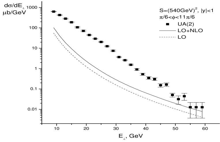
Figure 1: Transverse energy spectrum in $p{\bar{p}}$ collisions calculated within LO+NLO accuracy in perturbative QCD vs the experimental data by UA2 collaboration [68].

We see that the perturbative LO+NLO calculations start merging with the experimental data only around quite a large scale $E_{\perp}\sim 60$ GeV. It is interesting to note, that it is precisely around this energy, that the space of experimental events starts to be dominated by two-jet configurations [68]. This means that only starting from these transverse energies the assumptions behind the perturbative calculation (collinear factorization at leading twist, explicit account for all contributions of a given order in $\alpha_{s}$) are becoming adequate to the observed physical process of transverse energy production providing the required duality between the description of dominant configuration contributing to transverse energy production at this order in perturbation theory and the final state transverse energy carried by hadrons. At $E_{\perp}\leq 50$ GeV the calculated spectrum is in radical disagreement with the experimental one both in shape and magnitude calculated and observed spectrum is very large indicating the inadequacy of the considered $O(\alpha_{s}^{3})$ perturbative calculation in this domain. Let us mention here, that it is currently impossible to improve the results of the above calculation, because neither calculations of higher order nor infinite order resummation for this process are currently available.

In practical terms this means that additional model assumptions are needed to achieve agreement with experimental data strongly indicating that higher order corrections and higher twist effects have to be taken into account (in a necessarily model-dependent way) in order to describe them. In the popular Monte-Carlo generators such as PYTHIA [60] and HIJING [61] such effects as multiple binary parton-parton collisions, initial and final state radiation and transverse energy production during hadronization are included. In Fig. 2 we compare the same experimental data by UA(2) [68] with the spectrum calculated with HIJING event generator. To show the relative importance of different dynamical mechanisms, in Fig. 2 we plot the contributions from the hard parton scattering without initial and final state radiation, full partonic contribution and, finally, the transverse energy spectrum of final hadrons.

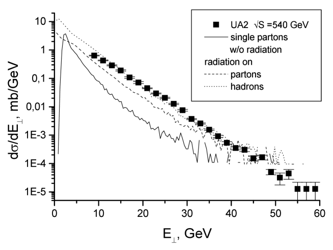
Figure 2: Transverse energy spectrum in $p{\bar{p}}$ collisions calculated in HIJING vs the experimental data by UA2 collaboration [68].

We see, that taking into account additional partonic sources such as, e.g., initial and final state radiation, allows to reproduce the (exponential) form of the spectrum, but still not the magnitude. The remaining gap is filled in by soft contributions due to transverse energy production from decaying stretched hadronic strings. Let us finally note, that the spectrum calculated in HIJING is somewhat steeper than the experimental one. Additional fine-tuning can be achieved by probing different structure functions.

The above results clearly demonstrate that in order to reproduce the experimentally observed transverse energy spectrum, one has to account for complicated mechanisms of parton production, such as initial and final state radiation accompanying hard parton-parton scattering, production of gluonic kinks by strings, as well as for nonperturbative transverse energy production at hadronization stage. This statement is a calorimetric analog of the well-known importance of the minijet component in describing the tails of the multiplicity distributions, [59] and [61].

Let us note that the result has straightforward implications for describing the early stages of heavy ion collisions. In most of the existing dynamical models of nucleus-nucleus collisions they are described as an incoherent superposition of nucleon-nucleon ones. As we have seen, to correctly describe the partonic configuration underlying the observed transverse energy flow in nucleon-nucleon collisions, mechanisms beyond conventional collinear factorization are necessary. This means that to estimate such quantities as, for example, parton multiplicity at some given timescale, a very careful analysis of various contributions is required.

4.1.2 Azimuthal pattern of transverse energy flow

Understanding the parton-related dynamical features of heavy ion collision calls for the analysis of experimentally observable quantities sensitive to particular features, distinguishing semihard parton dynamics from the soft hadronic one. One specific proposal in this direction was discussed in [69, 70]. The idea is that perturbative energy production generates asymmetric transverse energy flow due to its collimation along the directions fixed in the process of large momentum transfer.

To quantify the event-by-event asymmetry of transverse energy flow, let us consider the difference between the transverse energy deposited, in some rapidity window $y_{min}<y_{i}<y_{max}$, into two oppositely azimuthally oriented sectors with a specified angular opening $\delta\varphi$ each.

For convenience one can think of the directions of these cones as being ”up” and ”down” corresponding to some specific choice of the orientation of the system of coordinates in the transverse plane. All results are, of course, insensitive to the particular choice. Denoting now the transverse energy going into the ”upper” and ”lower” cones in a given event by $E_{\perp}^{\uparrow}(\delta\varphi)$ and $E_{\perp}^{\downarrow}(\delta\varphi)$ correspondingly, we can quantify the magnitude of the asymmetry in transverse energy production in a given event by

$$\delta E_{\perp}(\delta\varphi)\,=\,E_{\perp}^{\uparrow}(\delta\varphi)-E_{\perp}^{\downarrow}(\delta\varphi),$$ (99)

its statistical properties characterized by the corresponding probability distribution

$$P(\delta E_{\perp}|{\delta\varphi})\,=\,{d\,w(\delta E_{\perp}(\delta\varphi))\over d\,\delta E_{\perp}(\delta\varphi)}.$$ (100)

This distribution was calculated [70], in HIJING model, for central AuAu collisions at RHIC energy $\sqrt{s}=200\,{\rm GeV}$ and central PbPb collisions at LHC energy $\sqrt{s}=5.5\,{\rm TeV}$ for $\delta\varphi=\pi$. The distributions $P(\delta E_{\perp}|\pi)$ have been calculated both at partonic level and at the level of final hadrons with semihard interactions and quenching on and off. This allowed us to study the contribution of HIJING minijets and of the effects of their hadronization to the asymmetry in question. The resulting distributions are plotted in Figs. 3 and 4, for RHIC and LHC energies respectively with quenching turned on and the value of the minijet’s infrared cutoff $p_{0}=2\,{\rm GeV}$.

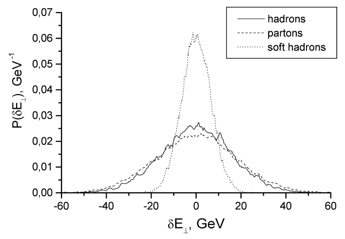
Figure 3: Probability distribution for azimuthal transverse energy disbalance in the unit rapidity window for AuAu collisions at RHIC energy $\sqrt{s}=200\,{\rm GeV}$, $p_{0}=2\,{\rm GeV}$, quenching on.

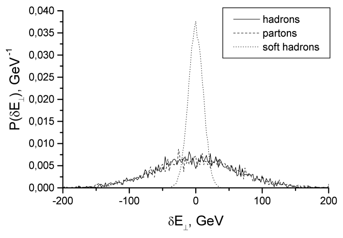
Figure 4: Probability distribution for azimuthal transverse energy disbalance in the unit rapidity window for PbPb collisions at LHC energy $\sqrt{s}=5.5\,{\rm TeV}$, $p_{0}=2\,{\rm GeV}$, quenching on.

The numerical values of the mean square deviation $\delta E_{\perp}$ characterizing the widths of the corresponding probability distributions in Figs. 3 and 4 are given in Table 1, where for completeness we also give the widths for the probability distributions with quenching turned off and with a larger value for the infrared cutoff $p_{0}=4\,{\rm GeV}$.

AA	$\sqrt{S}$, GeV	$p_{0}$, GeV	asymmetry	$\sqrt{\left<\delta E^{2}\right>}$
			hadrons (quenching on)	16
AuAu	200	2	hadrons (quenching off)	17
			partons	18
			soft hadrons	7
			hadrons (quenching on)	61
PbPb	5500	2	hadrons (quenching off)	71
			partons	65
			soft hadrons	15
			hadrons (quenching on)	69
PbPb	5500	4	partons	76
			soft hadrons	16

Table 1

The main conclusions that can be drawn from Figs. 3 and 4 and Table 1 are the following.

First, the magnitude of the azimuthal asymmetry as measured by the width of the probability distribution $P(\delta E_{\perp}|\delta\varphi)=dw(\delta E_{\perp}(\delta\varphi))/d\delta E_{\perp}(\delta\varphi)$ is essentially sensitive to semihard interactions (minijets). Switching off minijets, and thus restricting oneself to purely soft mechanisms, leads to a substantial narrowing of the asymmetry distribution; by the factor of 2.3 at RHIC and by the factor 4.1 at LHC energy respectively (these values correspond to the case of quenching being turned on).

Second, quite remarkably, the parton and final (hadronic) distributions of $\delta E_{\perp}$ in both cases practically coincide indicating that the contribution to transverse energy due to hadronization of the initial parton system is, with a high accuracy, additive and symmetric in between the oppositely oriented cones. Both conclusions show that the energy-energy correlation in Eq. (99) is a sensitive measure of the primordial parton dynamics that can be studied in calorimetric measurements in central detectors at RHIC and LHC.

Third, as expected, turning off quenching somewhat enhances the fluctuations. However, as seen from the table, numerically the effect is not important. This shows once again that the proposed asymmetry is really essentially determined by the earliest stage of the collision, when the primordial parton flux is formed.

Finally, from Table 1 we conclude that the studied asymmetry is not particularly sensitive to changing the value of the infrared cutoff $p_{0}$ and thus provides a robust signal for the presence of semihard dynamics deserving an experimental study.

4.1.3 Turbulent initial glue: impact parameter plane picture

In the previous paragraph we have discussed an event-by-event asymmetry of the transverse energy flow from the ”momentum” point of view. In a more detailed analysis a spatial pattern giving rise to this energy-momentum flux should be considered. Of particular interest is an event-by-event transverse energy generation pattern in the impact parameter plane. This question was first addressed in [86] - with strikingly interesting results.

The event-by-event transverse energy release pattern in the mixed-type models like HIJING is determined by two major factors. The first one is a distribution of the number of soft and (semi)hard inelastic collisions per unit transverse area. The second is the shape of the corresponding transverse momentum (energy) spectra. The convolution of the two distributions determines a shape of the transverse momentum and energy release. For broad resulting distributions one expects an intermittent turbulent-like spatial transverse energy distribution in the transverse plane. Most promising in this respect is of course the semihard partonic component. The distribution in the number of semihard inelastic interactions is quite broad, and the transverse energy spectra generated in these collisions are powerlike. It is precisely this combination that leads to the intermittent turbulent-like pattern of the primordial transverse energy release [86].

In [86] the transverse energy distribution for an ensemble of free-streaming gluons (taken from the HIJING parton event list) at zero rapidity $y=0$ (and thus at $z=0$) at proper time $\tau$ was taken to be

$${\cal E}(\tau,x_{\perp},z=0)\,=\,\sum_{k}{p_{\perp\,k}\over\tau}\,{(\tau p_{\perp\,k})^{2}\over 1+(\tau p_{\perp\,k})^{2}}\,\delta(x_{\perp}-x_{\perp\,k}(\tau))\,\delta(y_{k}),$$ (101)

where summation is over partons and the second factor in the right-hand side stands for the parton formation probability distribution.

To be meaningful, the transverse energy distribution should be considered in the coarse-grained coordinate space. More particularly, the size of the transverse cell is actually limited from below by the uncertainty principle $\delta r_{\perp}>1/\delta p_{\perp}$ and from above by causality (local horizon of the gluon in the comoving frame). At given $\tau$ this upper bound is simply given by $\delta r_{\perp}<\tau$, so that for large nuclei and small proper times the number of independent cells in the transverse plane can be quite large. The natural longitudinal size of the cell can be chosen as $|y|<1$.

The particular case considered in [86] was Au-Au collisions at RHIC energy $\sqrt{s}=200\,\,{\rm GeV}$. The snapshot of the transverse energy and transverse momentum distribution was taken at $\tau=0.5\,\,{\rm fm}$. The results turned out to be quite striking. On the background of the smooth uniformly distributed energy density ${\cal E}_{soft}\simeq 5\,\,{\rm GeV}$ one finds pronounced peaks (”hot spots”) with large energy densities ${\cal E}>20\,\,{\rm GeV}$ (corresponding to ${\cal E}_{hard}\succeq 15\,\,{\rm GeV}$) separated by distances of order $4-5\,\,{\rm fm}$, and the momentum field showed nontrivial vortex-like structure. A natural analogy suggested in [86] was that of the instabilities (turbulence) induced in the uniform ”soft” laminar flow by the minijet component.

The importance of the results of [86] go, in our opinion, far beyond the particular model (HIJING), collision energy, etc., considered in the paper. As we have mentioned on many occasions in the preceeding paragraphs, a consistent model of heavy ion collisions is necessarily a mix of soft and hard mechanisms. Any such mix will generate a turbulent-like intermittent picture analogous to the one discussed in [86].

4.2 Parton production and saturation in nuclear collisions

The cross-sections describing hard processes (e.g. high-$p_{\perp}$ jet production) are proportional to the product of incoming partonic flows. At high energies, when the saturation phenomenon becomes important, this customary picture has to be reconsidered. This analysis was first made in [87]. In particular it was shown, that because of saturation the multiplicity and transverse energy density of gluons produced at central rapidity scales as

$${dN\over dy} = 2\ AxG_{nucleon}(x,Q^{2}_{s}),$$

$${dE_{\perp}\over dy} = 2\ Q_{s}xG_{nucleon}(x,Q^{2}_{s}),$$ (102)

where $Q_{s}\sim\alpha A/R^{2}$ is a characteristic saturation scale at which gluon emission and recombination equilibrate. We see that the $A$ - counting in Eq. (4.2) is different from the naively expected perturbative factor $A^{2}$, and is more akin to the one in soft production models.

It is important to stress that the physical picture of gluon production, and thus that of the initially produced gluonic configuration, depends on the gauge used in the calculation. This was explicitly demonstrated in [73], where a calculation of the spectrum of gluons produced in p-A collisions was performed both in covariant and light-cone gauge. It turned out that the origin of A-dependent effects looks completely different in these two gauges: in the covariant gauge it is a rescattering of the produced gluon on the nucleons in the nucleus, and in the light-cone gauge it is a nonlinear interaction of gluons in the nuclear wavefunction. This explains a certain ambivalence with which an intuitive reasoning explaining the basic features of gluon production is formulated, see, e.g., [72]. Here it will be convenient to follow the ”light-cone gauge” way of reasoning, in which the number of produced gluons can be expected to be roughly proportional to the their ”pre-existing” number in the nuclear wavefunction [72].

4.2.1 Spectrum of produced gluons: analytical results

The qualitative ideas described in the previous subsection were further developed in [74], where the fully nonlinear analytical ansatz for the spectrum of gluons produced in the collision of two identical nuclei was suggested. The corresponding formula in [74] can be written as a two-dimensional integral integral in the transverse coordinate space. With logarithmic accuracy and for parametrically small transverse momenta $k^{2}_{\perp}<Q^{2}_{s}$ one can perform the two-dimensional integration over coordinates and obtain the following impressively simple expression for the gluon spectrum:

$${dN^{AA}\over d^{2}bdyd^{2}k_{\perp}}\,=\,{C_{F}\over\alpha\pi^{3}}\ {Q^{2}_{s}\over k^{2}_{\perp}}\left[{\rm e}^{-k^{2}_{\perp}/2Q^{2}_{s}}-{\rm e}^{-k^{2}_{\perp}/Q^{2}_{s}}\right].$$ (103)

From Eq. (103) there follows an important conclusion that (up to possible logarithmic factors neglected in the process of its derivation) the spectrum of gluons produced in nucleus-nucleus collision is finite in the limit $k^{2}_{\perp}/Q^{2}_{s}\to 0$:

$${dN^{AA}\over d^{2}bdyd^{2}k_{\perp}}\to{1\over\alpha}{C_{F}\over 2\pi^{3}},$$ (104)

thus ensuring an infrared-finite answer for quantities containing integration over transverse momenta such as, e.g., inelastic cross-section. This result is highly nontrivial. In the standard minijet scenarios based on collinear factorization such infrared finiteness can be ensured only by using brute force (an explicit infrared cutoff for a strongly divergent spectrum $\sim 1/k^{4}_{\perp}$). In p-A scattering, where nonlinear corrections related to the single participant nucleus are summed, the gluon spectrum still possesses a powerlike divergence at small momenta ($\sim 1/k^{2}_{\perp}$) [24, 74]. This shows that it is only a combination of all nonlinear effects in both colliding nuclei that ensures the infrared finiteness of the spectrum of produced gluons and the infrared finiteness of physical cross-sections computed from it.

The spectrum of Eq. (103) allows to make quantitative estimates relating the physical quantities to the saturation momentum more precise. In particular, the mean transverse momentum of produced gluons reads

$$\langle k^{2}_{\perp}\rangle\,=\,{1\over\ln 2}\ Q^{2}_{s}$$ (105)

We see, that the numerical value $\langle k^{2}_{\perp}\rangle$ is indeed very close to that of $Q^{2}_{s}$ supporting the intuitive picture advocated in [22] and [87, 72]. Performing in Eq. (103) integration over $k_{\perp}$, we obtain an expression for the gluon rapidity density in the transverse plane

$${dN^{AA}\over d^{2}bdy}\,=\,{1\over\alpha}{\ln 2\,C_{F}\over\pi^{2}}Q^{2}_{s}$$ (106)

It is illuminating to compare Eq. (106) with the expression for the density of gluons in the nuclear wavefunction computed in the same cylindrical geometry

$${dN^{MW}\over d^{2}bdy}\,=\,{1\over\alpha}{C_{F}\over 2\pi^{2}}Q^{2}_{s}$$ (107)

Comparing Eq. (106) with Eq. (107) we see that the density of produced gluons Eq. (106) is indeed proportional to the density of gluons in the nuclear wavefunction

$${dN^{AA}\over d^{2}bdy}\,=\,2\ln 2\,{dN^{MW}\over d^{2}bdy}$$ (108)

with the proportionality coefficient $2\ln 2\simeq 1.39$. From Eq. (106) one can also express the rapidity density of the produced gluons in terms of the nucleon structure function:

$${dN^{AA}\over dy}\,=\,\pi R_{A}^{2}{1\over\alpha}{\ln 2C_{F}\over\pi^{2}}Q^{2}_{s}\,=\,2\ln 2(V_{A}\rho)xG(x,Q^{2}_{s}),$$ (109)

where $V_{A}\sim A$ is a nuclear volume.

4.2.2 Parton production and saturation: numerical solution.

A natural extension of the philosophy of McLerran-Venugopalan approach to high energy heavy ion physics is to study, at the same quasiclassical level, the spectrum of gluons produced in collision of two nuclei, where the gluon spectrum is determined by the mode content of the gluon field created by two colliding nuclei [71]. In the pioneering paper [71] the spectrum of produced gluons was calculated to the leading order in perturbation theory. The answer contained a characteristic strong infrared divergence. Later these calculations were expanded in [75, 76, 77]. The problem at hand amounts to solving the Yang-Mills equations in the presence of external source current [71]:

$$J^{\mu}\,=\,\delta^{\mu+}\rho_{(1)}\delta(x^{-})+\delta^{\mu-}\rho_{(2)}\delta(x^{+})$$ (110)

corresponding to the two incident nuclei. Full analytical solution of the problem seems impossible, so a dedicated program of its numerical analysis was launched [78]-[85]. Assuming the boost invariance of the problem one deals with the problem of numerically solving the equations of motion in (2+1) classical hamiltonian chromodynamics on the lattice.

The result depends on three parameters,- charge $g$, color charge density $\mu$ and nuclear radius $R_{A}$, - through their dimensionless combination $\xi=g^{4}\pi R^{2}_{A}\mu^{2}$, so that for rapidity density of multiplicity and transverse energy of primordial glue one has

$${dE_{\perp}\over dy} = \mu\,\xi\,f_{E}(\xi)$$

$${dN\over dy} = \xi\,f_{N}(\xi).$$ (111)

In the weak field limit (more exactly, for $\xi<50$) all quantities are strongly dependent on $\xi$ and thus on the infrared cutoff. At $\xi\sim 100$ this dependence saturates.

One important issue to analyze is to check the (weak field) regime, in which the perturbative result of [71] should be valid. Most resent analysis shows, that the agreement can be reached only at very small values of scaling parameter $\xi<10$ [85]. As to the spectrum of produced gluons, it has an exponential ”thermal-looking” one at small energies [81, 85], but deviates from it at large energies [85].

The most important issue addressed by the numerical computation is, probably, that of a magnitude of occupation numbers of gluon modes $f_{g}$. The classical description that lies at the heart of the method is justified only at large $f_{g}\gg 1$. Although the situation here does not seem finally settled, for parameter values corresponding to RHIC energies, this condition is satisfied at best marginally.

4.2.3 Interpreting the RHIC data in Color Glass Condensate terms.

With a wealth of experimental data coming from RHIC it is tempting to test the ideas of Color Glass Condensate (saturation) physics in the simplest setting. Let us assume, that from the moment the Color Glass Condensate melts into physical glue, the produced gluons do not subsequently reinteract and convert into final hadrons without changing the kinematical characteristics of the energy-momentum flux (soft hadronization hypothesis). Then, by comparing with experimental data on charged multiplicity [98, 99, 100, 101] or multiplicity per participant [98] one can constrain parameters specifying the initially produced gluon configuration.

Consider for example the cylindrical nuclei model discussed in [74]. Then using, for example, the charged multiplicty density measured by PHOBOS in Au-Au collisions [98]

$${dN_{ch}^{AuAu}\over d\eta}\,=\,555\pm 12(stat)\pm 35(syst)$$ (112)

one obtains from Eq. (109), taking $\alpha_{s}=0.3$ and $\pi R_{A}^{2}=150$ fm, the estimate for the saturation momentum $Q_{s}$: $Q^{2}_{s}\approx 0.7\,\,{\rm GeV}^{2}$.

The relation of the results of numerical lattice computations described in paragraph 4.2.2 to the experimental data could be done analogously. For example, using the second of Eqn. (4.2.2), one can determine (for given $g$ and $R_{A}$) the value of $\mu$ and compute from the first of Eqn. (4.2.2) the transverse energy density. Using [85] $dN/dy\approx 1000$, one gets (for $g=2$ and $S_{A}=150$ fm²) $\mu=0.5$ GeV and $dE_{\perp}/dy=1.5\ {\rm GeV}\ dN/dy$.

A more elaborate way of estimating the characteristics of Color Glass Condensate from experimental data was suggested in [88, 89, 90]. The main novelty of this approach is to use a density of participating nucleons in the formula determining the saturation scale, so that

$$Q^{2}_{s}(s_{\perp},b_{\perp})\,=\,{4\pi^{2}N_{c}\over N^{2}_{c}-1}\ \alpha_{s}(Q^{2}_{s})\ xG(x,Q^{2}_{s})_{nucleon}\ {\rho_{part}(s_{\perp},b_{\perp})\over 2}$$ (113)

where $\rho_{part}(s_{\perp},b_{\perp})$ is a density of participant nucleons as a function of the collision impact parameter $b_{\perp}$ and the coordinate in the transverse plane $s_{\perp}$. The substitution of $\rho_{part}$ into equation determining a saturation scale presents a highly nontrivial hypothesis on, in fact, non-perturbative geometry present behind gluon production. The resulting relation between multiplicity per participant and saturation momentum reads [88, 89, 90, 95, 97]:

$$\left\langle{2\over N_{part}}\ {dN_{ch}\over dy}\right\rangle\simeq{2\over 3}\ c\ xG(x,\langle Q^{2}_{s}\rangle),$$ (114)

where $c$ is a proportionality coefficient between the gluon spectrum and nuclear wavefunction discussed in paragraph 4.2.1, averaging in the left-hand side is over events having different number of participants and $\langle Q^{2}_{s}\rangle$ denotes averaging over the impact parameter. Experimentally $2/N_{part}dN_{ch}/dy\simeq 3.8$, so that from Eq. (114) one can estimate the (average) saturation momentum $Q_{s}$. Without invoking additional assumptions the typical value for $Q^{2}_{s}$ on gets from Eq. (114) is also not too big: $Q^{2}_{s}\simeq 0.5-0.7$ GeV².

4.3 Interaction effects. On the way to thermalization?

Up to now we have discussed only the properties of the initially produced gluon system appearing immediately after the coherence of the wavefunctions of incident nuclei is broken by the collision and, as a consequence, entropy in the form of the physical (mainly gluonic) fields is produced. Before the energy-momentum flux of these fields converts into that of final hadrons hitting detectors it could, however, be essentially transformed by interaction effects. The question that has particularly shaped the high energy heavy ion physics is whether the reinteraction of produced parton matter could lead to its thermalization into quark-gluon plasma, thus allowing to reproduce, in the laboratory, conditions that existed in the Early Universe. In this paragraph we shall briefly review the recent progress in describing the real time evolution of an interacting (dense) gluon system.

Broadly speaking, one could classify reinteraction effects into two categories.

First, if a strong physical gluon field is produced, it can evolve (in real time) according to the nonlinear Yang-Mills equations of motion. This regime is possible up until the occupation numbers of the field modes become small. Schematically, the occupation numbers $f$ should satisfy $1<f<1/\alpha_{s}$. Such nonlinear evolution could, in principle, lead to all kind of exciting scenarios typical for the nonlinear field dynamics - from appearence of collective dynamical instabilities to chaotization and formation of solitons.

Second, one could describe the reinteraction of produced physical glue in terms borrowed from kinetic theory . This possibility has been discussed, in relation to saturation physics in nuclear collisions, in a number of recent publications [91]-[95].

The simplest way to analyze gluon reinteraction effects is to use a Boltzmann equation formalism at a binary scattering level [91, 92, 93]. Calculation of equilibration time in this approximation produce a parametrically big estimate $\tau_{eq}\sim{\rm exp}(1/\sqrt{\alpha_{s}})1/Q_{s}$. The equilibration rate is low because the momentum transfer in the system is not effective: the transverse momenta exchanged in gluon interactions are small - of order of the infrared cutoff (screening Debye mass).

The main motivation for developing a saturation physics approach is a very dense system of primordial gluons that is, presumably, formed at the initial stage of high energy heavy ion collision. To produce a more reliable description for gluon reinteraction and their possible equilibration a kinetic approach that that is more appropriate for (initially) dense systems is called for. Such approach was developed in [94, 95], where the kinetic equation formalism taking into account inelastic processes in the third order in gluon density was constructed and employed. The resulting reinteraction scenario described in [94, 95] is quite complex and involves several stages. The corresponding proper time scales are $\tau\sim(\tau_{0},\alpha_{s}^{-3/2}\tau_{0},\alpha_{s}^{-5/2}\tau_{0},\alpha_{s}^{-13/5}\tau_{0}))$, where $\tau_{0}=1/Q_{s}$.

First, at $\tau\sim\tau_{0}$, physical glue is freed from the nuclear wavefunctions. This is a dense system of (semi)hard gluons having transverse momenta of order of $Q_{s}$ and occupation number of order $1/\alpha_{s}$. The system expands, and at $\tau\sim\alpha_{s}^{-3/2}\tau_{0}$ the occupation numbers of semihard primordial gluons become small, so that a standard description in terms of Boltzmann equation can be applied.

In the time interval $\alpha_{s}^{-3/2}\tau_{0}<\tau<\alpha_{s}^{-5/2}\tau_{0}$ inelastic interactions of semihard gluons produce soft gluons with momenta $k_{\perp}\sim\alpha_{s}^{1/2}$. At the end of this interval the densities of hard and soft gluon components equalizes.

At $\tau>\alpha_{s}^{-5/2}\tau_{0}$ the soft gluon subsystem thermalizes. Its temperature subsequently undergoes a linear increase through the energy loss of the remaining semihard modes in the hot soft gluon medium until it reaches, at $\tau\sim\alpha_{s}^{-13/5}\tau_{0}$, its maximal value $T\sim\alpha_{s}^{2/5}Q_{s}$. At this timescale semihard glue disappears and the gluon system is fully equilibrated.

Detailed discussion of RHIC data in the context of the above-described scenario can be found in [95].

Let us note, that the validity of the scenario described in [94, 95] is based on some quite restrictive assumptions. For example, for equilibration time $\alpha_{s}^{-13/5}\tau_{0}$ to be less than the ”binary” one ${\rm exp}(1/\sqrt{\alpha_{s}})$, the coupling constant should be really small, $\alpha_{s}<0.004$. Also - especially at RHIC energies, when $Q_{s}\sim 1\,{\rm GeV}^{2}$ and realistic values of the coupling constant $\alpha_{s}\sim 0.3$, the transverse momenta of the soft gluons produced to the second stage $k_{\perp}\sim\alpha_{s}^{1/2}\tau_{0}$ are in fact of order $\Lambda_{QCD}$, so that to describe the evolution of the soft gluon subsystem perturbative methods could turn out to be insufficient.

5 Conclusion

In the present review we have discussed some aspects of an exciting and rapidly developing field of nonlinear QCD physics in ultrarelativistic heavy ion collisions. Research in this field deals both with fundamental theoretical issues, such as unitarity of strong interactions at high energies, and with the challenge of describing experimental data coming, at present, from RHIC and expected exciting physics of forthcoming experiments at LHC.

Acknowledgements

I am indebted to I.M. Dremin, E. Iancu, A. Kovner and L. McLerran for reading the manuscript and useful comments and suggestions.

References

- [1] X.-N. Wang, Phys. Repts 280 (1997), 287
- [2] E. Iancu, A. Leonidov, L. McLerran, The Colour Glass Condensate: An Introduction, [arXiv:hep-ph/0202270]
- [3] E. Iancu, R. Venugopalan, The Color Glass Condensate and HIgh Energy Scattering in QCD, [arXiv:hep-ph/0303204]
- [4] A.B. Kaidalov, Surveys High Energy Physics 13 (1999), 265; Nucl Phys. Proc. Suppl. A75 (1999),81
- [5] A.B. Kaidalov, K.A. Ter-Martirosyan, Sov. Journ. Nucl. Phys. 40 (1984), 211
- [6] V.A. Khoze, W. Ochs, Int. Journ. Mod. Phys. A12 (1997), 2949
- [7] I.M. Dremin, J.W. Gary, Phys. Repts. 349 (2001), 301
- [8] I.M. Dremin, Physics-Uspekhi 45 (2002), 507
- [9] A.B. Kaidalov, Physics-Uspekhi, to appear
- [10] V. Emelyanov et. al., Physics-Uspekhi, to appear
- [11] I.I. Royzen, E.L. Feinberg, O.D. Chernavskaya, Physics-Uspekhi, to appear
- [12] E.A. DeWolf, I.M. Dremin, W. Kittel, Phys. Rep. 270 (1996), 1
-
[13]
V.N. Gribov, L.N. Lipatov, Sov. Journ. Nucl. Phys. 15
(1972), 438;
G. Altarelli, G. Parisi, Nucl. Phys. B126 (1977), 298;
Yu.L. Dokshitzer, Sov. Phys. JETP 46 (1977), 641. -
[14]
L.N. Lipatov, Sov. Journ. Nucl. Phys. 23 (1976),
338;
E.A. Kuraev, L.N. Lipatov, V.S. Fadin, Sov. Phys. JETP 45 (1977), 199;
Ya.Ya. Balitsky, L.N. Lipatov, Sov. Journ. Nucl. Phys. 28 (1978), 822. - [15] L. V. Gribov, E. M. Levin, M. G. Ryskin, Phys. Rept. 100 (1983), 1.
- [16] A.H. Mueller, Jian-wei Qiu, Nucl. Phys. B268 (1986), 427.
- [17] L.L. Frankfurt, M. I. Strikman, Phys. Rept. 160 (1988), 235.
- [18] E.M. Levin, M.G. Ryskin, Phys. Repts. 189 (1990), 267.
- [19] A.P. Bukhvostov, G.V. Frolov, L.N. Lipatov, E.A. Kuraev, Nucl. Phys. B258 (1985), 610.
- [20] L. N. Lipatov, Phys. Rept. 286 (1997), 131.
- [21] L. N. Lipatov, Nucl. Phys B452 (1995), 369.
-
[22]
L. McLerran, R. Venugopalan, Phys. Rev. D49 (1994),
3352;
ibid. D50 (1994), 2225. - [23] J. Jalilian-Marian, A. Kovner, L. McLerran, H. Weigert, Phys.Rev. D55 (1997), 5414.
- [24] Yu.V. Kovchegov, A.H. Mueller, Nucl. Phys. B259 (1998), 451.
-
[25]
C.S. Lam, G. Mahlon, Phys. Rev. D52 (2000), 114023;
ibid. D64 (2001), 016004. -
[26]
A. Ayala, J. Jalilian-Marian, L. McLerran, R. Venugopalan, Phys. Rev. D52 (1995), 2935;
ibid. D53 (1996), 458. - [27] J. Jalilian-Marian, A. Kovner, A. Leonidov, H. Weigert, Nucl. Phys. B504 (1997), 415.
- [28] J. Jalilian-Marian, S. Jeon, R. Venugopalan, Phys. Rev. D63 (2001), 036004
- [29] A. Leonidov, Nonlinear Evolution Equations in QCD, Fradkin Conference.
- [30] J. Jalilian-Marian, A. Kovner, A. Leonidov, H. Weigert, Phys. Rev. D59 (1999), 014014.
- [31] E. Iancu, A. Leonidov, L. McLerran, Nucl. Phys. A692(2001), 583.
- [32] E. Iancu, A. Leonidov, L. McLerran, Phys. Lett. B510 (2001), 45.
- [33] E. Fereiro, E. Iancu, A. Leonidov, L. McLerran, Nucl. Phys. A703 (2002), 489.
- [34] J. Jalilian-Marian, A. Kovner, H. Weigert, Phys. Rev. D59 (1999), 014015.
- [35] A. Kovner, G. Milhano, Phys.Rev. D61 (2000), 014012.
- [36] E. Iancu, L. McLerran, Phys. Lett. B510 (2001), 145
- [37] A.H. Mueller, Phys. Lett. B523 (2001), 243.
-
[38]
J. Bartels, Nucl. Phys. B175 (1980),365;
J.Kwiecinski, M. Praszalowicz, Phys. Lett. B94 (1980), 413. - [39] I. Balitsky, Nucl. Phys. B463(1996), 99.
-
[40]
Yu. Kovchegov, Phys. Rev. D60(1999), 034008;
ibid. D61(2000), 074018. - [41] M. Braun, Eur. Phys. Journ. C16 (2000), 337.
- [42] H. Weigert, Nucl. Phys. A703 (2002), 823
- [43] A.H. Mueller, Phys. Lett. B523 (2001), 243
- [44] A.H. Mueller, Nucl. Phys. B558 (1999), 285
- [45] K. Golec-Biernart, M. Wustoff, Phys. Rev. D60 (1999), 114023
-
[46]
E. Levin, K. Tuchin, Nucl. Phys. B573 (2000), 833;
Nucl. Phys. bf A693 (2001), 787 - [47] E. Iancu, K. Itakura, L. McLerran, Nucl. Phys. A708 (2002), 327
- [48] E. Iancu, K. Itakura, L. McLerran, “ Gaussian effective theory for gluon saturation ” , [ hep-ph/0212123 ]
- [49] A. Kovner, J. G. Milhano, H. Weigert, Phys. Rev. D62, (2000), 114005.
- [50] J. Jalilian-Marian, A. Kovner, A. Leonidov, H. Weigert, Phys. Rev. D59 (1999) ,034007.
- [51] E. Ferreiro, E. Iancu, K. Itakura, L. McLerran, Nucl. Phys. A710 (2002), 373
- [52] A. Kovner, U. Wiedemann, Phys. Rev. D64 (2001), 114002
- [53] A. Kovner, U. Wiedemann, Phys. Rev. D66 (2002), 051502
- [54] A. Kovner, U. Wiedemann, Phys. Rev. D66 (2002), 034031
- [55] A. Kovner, U. Wiedemann, Phys. Lett. B551 (2003), 511
- [56] M. Jacob, P.V. Landshoff, Mod. Phys. Lett. A1 (1986), 657
- [57] K. Kajantie, P.V. Landshoff and J. Lindfors, Phys. Rev. Lett. 59 (1987), 2527
- [58] K.J. Eskola, K. Kajantie and J. Lindfors, Nucl. Phys. B323 (1989), 37
- [59] T. Sjostrand and M. van der Zijl, Phys. Rev. D36 (1987), 2019
- [60] T. Sjostrand, Comput. Phys. Commun. 82 (1994), 74;
-
[61]
X.-N. Wang and M. Guylassy, Phys. Rev. D44 (1991),
3501;
D45 (1992), 844;
Comput. Phys. Commun. 83 (1994), 307 - [62] X.-N. Wang, Phys. Rev. D46 (1992), R1900; D47 (1993), 2754
- [63] M. Guylassy, X.-N. Wang, Phys. Rev. Lett. 86 (2001), 3496
- [64] A. Leonidov, ”On transverse energy production in hadron collisions” , [ ArXiv:hep-ph/0005010 ]
- [65] D. Soper, ”Jet observables in theory and reality” [hep-ph/9706320]
- [66] Z. Kunszt and D.E. Soper, Phys. Rev. D46 (1992), 192
- [67] A. Leonidov, D. Ostrovsky, Eur. Phys. Journ. C11 (1999), 495
- [68] UA2 Collaboration, M. Banner et. al., Phys. Lett. B118 (1982), 203
- [69] A. Leonidov, D. Ostrovsky, Eur. Phys. Journ. C16 (2000), 683
- [70] A. Leonidov, D. Ostrovsky, Phys. Rev. C63 (2001), 037901
- [71] A. Kovner, L. McLerran and H. Weigert, Phys. Rev. D52 (1995), 3809; ibid. D52 (1995), 6231
- [72] A.H. Mueller, Nucl. Phys. B572 (2000), 227
- [73] A.H. Mueller, Yu. Kovchegov, Nucl. Phys. (1999),
-
[74]
Yu. Kovchegov, Nucl. Phys A692 (2001), 557;
ibid. A698 (2002), 619 - [75] Yu. V.Kovchegov and D.H. Rischke, Phys. Rev. C56 (1997), 1084
- [76] S.G. Matinyan, B. Mueller and D.H. Rischke, Phys. Rev. C56 (1997), 1927; ibid. C57 (1998), 2197
- [77] M. Gyulassy and L. McLerran, Phys. Rev. C56 (1997), 2219
- [78] A. Krasnitz, R. Venugopalan, Nucl. Phys. B557 (1999), 237
- [79] A. Krasnitz, R. Venugopalan, Phys. Rev. Lett. 84 (2000), 4309
- [80] A. Krasnitz, R. Venugopalan, Phys. Rev. Lett. 86 (2001), 1717
- [81] A. Krasnitz, Y. Nara, R. Venugopalan, Phys. Rev. Lett. 87 (2001), 192302
- [82] A. Krasnitz, R. Venugopalan, Nucl. Phys. A698 (2002), 209c
- [83] A. Krasnitz, Y. Nara, R. Venugopalan, Phys. Lett. B554 (2003), 21
- [84] A. Krasnitz, Y. Nara, R. Venugopalan, Nucl. Phys. A717 (2003), 268
- [85] T. Lappi, Phys. Rev. C67 (2003), 054903
- [86] M. Gyulassy, D.H. Rischke, B. Zhang, Nucl. Phys. A613 (1997), 397
- [87] J.P. Blaizot and A.H. Mueller, Nucl. Phys. B289 (1987), 847
- [88] D. Kharzeev, M. Nardi, Phys. Lett. B507 (2001), 121
- [89] D. Kharzeev, E. Levin, Phys. Lett. B523 (2001), 79
- [90] D. Kharzeev, E. Levin, M. Nardi, [ArXiv:hep-ph/0111315]
- [91] A.H. Mueller, Phys. Lett. B475 (2000), 220
- [92] J. Bjoraker, R. Venugopalan, Phys. Rev. C63 (2000), 024609
- [93] J. Serreau, D. Schiff, JHEP 0111 (2001), 039
- [94] R. Baier, A.H. Mueller, D. Schiff, D.T. Son, Phys. Lett. B502 (2001), 51
- [95] R. Baier, A.H. Mueller, D. Schiff, D.T. Son, Phys. Lett. B539 (2002), 46
- [96] A.H. Mueller, D.T. Son, ”On the equivalence between the Boltzmann equation and classical field theory at large occupation numbers” , [ ArXiv:hep-ph/0208278 ]
- [97] A. Mueller, ”QCD in nuclear collisions” , [ ArXiv:hep-ph/0208278 ]
-
[98]
B.B. Back et al. (PHOBOS Collaboration), Phys. Rev. Lett. 85 (2000), 3100;
Phys. Rev. Lett. 88 (2002), 022302 -
[99]
K. Adcox et al., (PHENIX Collaboration), Phys. Rev. Lett. 86 (2001), 51;
Phys. Rev. Lett. 87 (2001), 052301 - [100] I.G. Bearden et al., Phys. Lett. B523 (2001), 227
- [101] C. Adler et al., Phys. Rev. Lett. 87 (2001), 0112303