One-loop Radiative Corrections to the $\rho$ Parameter
in the Littlest Higgs Model

Abstract

We perform a one-loop analysis of the $\rho$ parameter in the Littlest Higgs model, including the logarithmically enhanced contributions from both fermion and scalar loops. We find the one-loop contributions are comparable to the tree level corrections in some regions of parameter space. The fermion loop contribution dominates in the low cutoff scale $f$ region. On the other hand, the scalar loop contribution dominates in the high cutoff scale $f$ region and it grows with the cutoff scale $f$. This in turn implies an upper bound on the cutoff scale. A low cutoff scale is allowed for a non-zero triplet VEV. Constraints on various other parameters in the model are also discussed. The role of triplet scalars in constructing a consistent renormalization scheme is emphasized.

I Introduction

The Standard Model(SM) requires a Higgs boson to explain the generation of fermion and gauge boson masses. Precision electroweak measurements suggest that the Higgs boson must be relatively light, $m_{H}<219~{}GeV$ lep (2003). Currently, experimental data overwhelmingly support the SM with a light Higgs boson. The simplest version of the Standard Model with a single Higgs boson, however, has the theoretical problem that the Higgs boson mass is quadratically sensitive to any new physics which may arise at high energy scales. Fine tuning and naturalness arguments suggest that the scale at which this new physics enters should be on the order of a TeV.

Supersymmetry addresses the quadratic sensitivity of the SM to high mass scales by introducing superpartners to the ordinary fields. The contributions of the superpartners to the Higgs mass explicitly cancel the quadratic dependence of the Higgs mass on the high mass scales. Little Higgs (LH) models Arkani-Hamed et al. (2001); Arkani-Hamed et al. (2002b, c, a); Low et al. (2002); Kaplan and Schmaltz (2003); Chang and Wacker (2003); Skiba and Terning (2003); Chang (2003) are a new approach to understanding the hierarchy between the $TeV$ scale of possible new physics and the electroweak scale, $v=246~{}GeV=(\sqrt{2}G_{F})^{-1/2}$. These models have an expanded gauge structure at the TeV scale which contains the Standard Model $SU(2)\times U(1)$ electroweak gauge groups. The LH models are constructed such that an approximate global symmetry prohibits the Higgs boson from obtaining a quadratically divergent mass until at least two loop order. The Higgs boson is a pseudo-Goldstone boson Dimopoulos and Preskill (1982); Kaplan and Georgi (1984); Kaplan et al. (1984); Georgi and Kaplan (1984); Georgi et al. (1984); Dugan et al. (1985); Banks (1984) resulting from the spontaneous breaking of the approximate global symmetry and so is naturally light. The Standard Model then emerges as an effective theory which is valid below the scale $f$ associated with the spontaneous breaking of the global symmetry.

Little Higgs models contain weakly coupled TeV scale gauge bosons from the expanded gauge structure, which couple to the Standard Model fermions. In addition, these new gauge bosons typically mix with the Standard Model $W$ and $Z$ gauge bosons. Modifications of the electroweak sector of the theory, however, are severely restricted by precision electroweak data and require the scale of the little Higgs physics, $f$, to be in the range $f>1-6~{}TeV$ Csaki et al. (2003a); Hewett et al. (2002); Csaki et al. (2003b); Kribs (2003); Gregoire et al. (2003); Perelstein et al (2003); Casalbuoni et al (2003); Kilian and Reuter (2003), depending on the specifics of the model. The LH models also contain expanded Higgs sectors with additional Higgs doublets and triplets, as well as a new charge $2/3$ quark, which have importance implications for precision electroweak measurements.

In this paper, we analyze the contributions of the heavy fermions and scalars to the isospin violating $\rho$ parameter. We include the logarithmically enhanced loop corrections due to the scalar triplet which is present in such models. In Section II, we review the LH models. Section III contains a description of our calculation, while numerical results are presented in Section IV. Details of the calculation are relegated to the appendices.

II Basics of Little Higgs Models

The Little Higgs model has been described in detail elsewhere, but we include a brief description of the model here in order to clarify our notation. [Our discussion follows Ref. Han et al. (2003).] The minimal version, the ”littlest Higgs model” (LLH) Arkani-Hamed et al. (2002a) is a non-linear sigma model based on an SU(5) global symmetry, which contains a gauged $[SU(2)\otimes U(1)]_{1}\otimes[SU(2)\otimes U(1)]_{2}$ symmetry as its subgroup. We concentrate on this model here, although many alternatives have been proposed Low et al. (2002); Kaplan and Schmaltz (2003); Chang and Wacker (2003); Skiba and Terning (2003); Chang (2003).

The global SU(5) symmetry of the LLH model is broken down to SO(5) by the vacuum expectation value (VEV) of a sigma field Arkani-Hamed et al. (2002a),

$$\Sigma_{0}=\left(\begin{array}[]{ccc}&&\mathbb{I}\\ &1&\\ \mathbb{I}&&\end{array}\right)\quad,$$ (1)

where $\mathbb{I}$ is a $2\times 2$ identity matrix and $\langle\Sigma_{0}\rangle\sim f$. In addition, the VEV of the sigma field breaks the gauged symmetry $[SU(2)\otimes U(1)]_{1}\otimes[SU(2)\otimes U(1)]_{2}$ to its diagonal subgroup, $SU(2)\times U(1)$, which is then identified as the SM gauge group. The breaking of the global symmetry, $SU(5)\rightarrow SO(5)$, leaves $14$ Goldstone bosons, $\Pi\equiv\pi^{a}X^{a}$, which can be written as

$$\Sigma=e^{i\Pi/f}\Sigma_{0}e^{i\Pi^{T}/f}=\Sigma_{0}+\frac{2i}{f}\Pi\Sigma_{0}+\mathcal{O}(1/f^{2}),$$ (2)

where $X^{a}$ correspond to the broken $SU(5)$ generators. Four of these Goldstone bosons become the longitudinal components of the broken gauge symmetry, while the remaining ten pseudo-Goldstone bosons can be parameterized as Arkani-Hamed et al. (2002a),

$$\Pi=\left(\begin{array}[]{ccc}&h^{\dagger}/\sqrt{2}&\Phi^{\dagger}\\ h/\sqrt{2}&&h^{\ast}/\sqrt{2}\\ \Phi&h^{T}/\sqrt{2}&\end{array}\right),$$ (3)

where $h$ is identified as the SM Higgs doublet, $h=(h^{+},\;h^{0})$, and $\Phi$ is a complex SU(2) triplet with hypercharge $Y=2$,

$$\Phi=\left(\begin{array}[]{cc}\Phi^{++}&\Phi^{+}/\sqrt{2}\\ \Phi^{+}/\sqrt{2}&\Phi^{0}\end{array}\right).$$ (4)

The existence of an $SU(2)$ triplet is a general feature of models of this type.

The Lagrangian is given by

$$\mathcal{L}=\mathcal{L}_{k}+\mathcal{L}_{Yuk}\quad,$$ (5)

where $\mathcal{L}_{k}$ contains the kinetic terms of all fields and $\mathcal{L}_{Yuk}$ describes the Yukawa interactions. The gauge bosons acquire their masses through the kinetic terms of the $\Sigma$ field

$$\mathcal{L}_{k}=\frac{f^{2}}{8}\mbox{Tr}\{(D_{\mu}\Sigma)\,(D^{\mu}\Sigma)^{\dagger}\}\quad,$$ (6)

where the covariant derivative of the $\Sigma$ field is defined as

$$D_{\mu}\Sigma=\partial_{\mu}\Sigma-i\sum_{j}[\,g_{j}W_{j}^{a}(Q_{j}^{a}\Sigma+\Sigma Q_{j}^{a}{}^{T})+g_{j}^{{}^{\prime}}B_{j}(Y_{j}\Sigma+\Sigma Y_{j}^{T})\,]\quad.$$ (7)

The SU(2) gauge fields are given by $W_{j}=\sum_{a=1}^{3}\;W_{j}^{\mu\,a}Q_{j}^{a}$, and the U(1) gauge fields are $B_{j}=B_{j}^{\mu}Y_{j}$, with gauge couplings $g_{1},g_{2}$ and $g_{1}^{\prime},g_{2}^{\prime}$. (The $SU(2)$ and hypercharge, $Y_{j}$ assignments can be found in Ref. Arkani-Hamed et al. (2002a)).

The $\Sigma_{0}$ VEV generates masses and mixing between the gauge bosons. The heavy gauge boson mass eigenstates are given by,

$$W_{H}^{a}=-cW_{1}^{a}+sW_{2}^{a},\quad B_{H}^{a}=-c^{\prime}B_{1}+s^{\prime}B_{2}\quad,$$ (8)

with masses Csaki et al. (2003a); Hewett et al. (2002); Han et al. (2003)

$$M_{\scriptstyle W_{H}}^{2}=\frac{f^{2}}{4}(g_{1}^{2}+g_{2}^{2}),\quad M_{\scriptstyle B_{H}}^{2}=\frac{f^{2}}{20}(g_{1}^{{}^{\prime}2}+g_{2}^{{}^{\prime}2})\quad.$$ (9)

The orthogonal combinations of gauge bosons are identified as the SM $W$ and $B$, with couplings Csaki et al. (2003a); Hewett et al. (2002); Han et al. (2003),

$$g=g_{1}s=g_{2}c,\quad g^{\prime}=g_{1}^{\prime}s^{\prime}=g_{2}^{\prime}c^{\prime}\quad.$$ (10)

The mixing between the two SU(2)’s (U(1)’s) is described by the parameters $s$ and $s^{\prime}$ Csaki et al. (2003a); Hewett et al. (2002); Han et al. (2003),

$$s=\frac{g_{2}}{\sqrt{g_{1}^{2}+g_{2}^{2}}},\quad s^{\prime}=\frac{g_{2}^{\prime}}{\sqrt{g_{1}^{\prime 2}+g_{2}^{\prime 2}}}\quad.$$ (11)

(and $c=\sqrt{1-s^{2}}$, $c^{\prime}=\sqrt{1-s^{\prime 2}}$.) The coupling of fermions to the photon is then given by Csaki et al. (2003a); Hewett et al. (2002); Han et al. (2003),

$$e = gs_{W}$$ (12)

$$s_{W} = \frac{g^{\prime}}{\sqrt{g^{2}+g^{\prime 2}}}$$ (13)

$$c_{W} = \frac{g}{\sqrt{g^{2}+g^{\prime 2}}}\quad.$$ (14)

In the Yukawa sector, a new vector-like charge $2/3$ fermion is introduced to cancel the quadratic sensitivity of the Higgs mass to the top quark loops. This cancellation fixes the Yukawa interactions Arkani-Hamed et al. (2002a); Han et al. (2003),

$$\mathcal{L}_{Yuk}={1\over 2}\lambda_{1}f\epsilon_{ijk}\epsilon_{xy}\chi_{i}\Sigma_{jx}\Sigma_{ky}u_{3}^{\prime}{}^{c}+\lambda_{2}f\tilde{t}\tilde{t}^{c}+h.c.\quad,$$ (15)

where $t_{3}$ is the SM top quark, $u_{3}^{\prime}$ is the SM right-handed top quark, $({\tilde{t}},\tilde{t}^{\prime c})$ is a new charge $2/3$ vector-like quark and ${\chi}=(b_{3},\;t_{3},\;\tilde{t})$. Expanding the $\Sigma$ field in terms of its component fields, the mass terms of the fermions are Arkani-Hamed et al. (2002a); Hewett et al. (2002); Han et al. (2003),

$$\mathcal{L}_{Yuk} = f\biggl{[}\sqrt{\lambda_{1}^{2}+\lambda_{2}^{2}}-\frac{\lambda_{1}^{2}}{2\sqrt{\lambda_{1}^{2}+\lambda_{2}^{2}}}\frac{v^{2}}{f^{2}}\biggr{]}\tilde{t}\tilde{t}^{c}-\frac{i\lambda_{1}^{2}v}{\sqrt{\lambda_{1}^{2}+\lambda_{2}^{2}}}t_{3}\tilde{t}^{c}$$

$$-\frac{i\lambda_{1}\lambda_{2}v}{\sqrt{\lambda_{1}^{2}+\lambda_{2}^{2}}}t_{3}u_{3}^{c}-\frac{\lambda_{1}\lambda_{2}}{2\sqrt{\lambda_{1}^{2}+\lambda_{2}^{2}}}\frac{v^{2}}{f^{2}}\tilde{t}u_{3}^{c}\quad.$$

The following mass eigenstates are obtained after diagonalizing the above mass terms Hewett et al. (2002); Han et al. (2003),

$$t_{L} = t_{3}+ix_{L}\frac{v}{f}\tilde{t}$$ (17)

$$T_{L} = \tilde{t}-ix_{L}\frac{v}{f}t_{3}$$ (18)

$$t_{R}^{c} = u_{3}^{c}=\frac{1}{\sqrt{\lambda_{1}^{2}+\lambda_{2}^{2}}}(-\lambda_{1}\tilde{t}^{\,{}^{\prime}c}+\lambda_{2}u_{3}^{{}^{\prime}c})$$ (19)

$$T_{R}^{c} = \tilde{t}^{c}=\frac{1}{\sqrt{\lambda_{1}^{2}+\lambda_{2}^{2}}}(\lambda_{2}\tilde{t}^{\,{}^{\prime}c}+\lambda_{1}u_{3}^{{}^{\prime}c})\quad.$$ (20)

We express our results in terms of $x_{L}$, which parameterizes the mixing between $t_{3}$ and $\tilde{t}$; it is given by Hewett et al. (2002); Han et al. (2003)

$$x_{L}=\frac{\lambda_{1}^{2}}{\lambda_{1}^{2}+\lambda_{2}^{2}}\quad.$$ (21)

The tree level $t\overline{t}h$ Yukawa coupling is now Hewett et al. (2002); Han et al. (2003),

$$y_{t}\,=\,{m_{t}\over v}\,=\,\frac{i\lambda_{1}\lambda_{2}}{\sqrt{\lambda_{1}^{2}+\lambda_{2}^{2}}}\,\biggl{[}\,1+\frac{v^{2}}{2f^{2}}\frac{\lambda_{1}^{2}}{\lambda_{1}^{2}+\lambda_{2}^{2}}(1+\frac{\lambda_{1}^{2}}{\lambda_{1}^{2}+\lambda_{2}^{2}})\,\biggr{]}.$$ (22)

In the limit that the cut-off scale $f$ goes to infinity, the coupling Hewett et al. (2002); Han et al. (2003)

$$y_{t}\,=\,\frac{i\lambda_{1}\lambda_{2}}{\sqrt{\lambda_{1}^{2}+\lambda_{2}^{2}}}$$ (23)

is identified as the top quark Yukawa coupling of the SM.

The one-loop quadratically divergent contributions to the Coleman-Weinberg potential due to the scalars and fermions are given by Arkani-Hamed et al. (2002a); Han et al. (2003)

$$\mathcal{L}_{s} = \frac{a}{2}f^{4}\{g_{j}^{2}\sum_{a}\;Tr[(Q_{j}^{a}\Sigma)+(Q_{j}^{a}\Sigma){}^{\ast}]+g_{j}^{\prime 2}Tr\;[(Y_{j}\Sigma)+(Y_{j}\Sigma){}^{\ast}]\}$$ (24)

$$\mathcal{L}_{f} = -\frac{a^{\prime}}{4}\lambda_{1}^{2}f^{4}\epsilon^{wx}\epsilon_{yz}\epsilon^{ijk}\epsilon_{kmn}\Sigma_{iw}\Sigma_{jx}\Sigma^{\ast my}\Sigma^{\ast nz}\quad.$$ (25)

where $a$ and $a^{\prime}$ are unknown coefficients parameterizing physics from the Ultra-Violet (UV) completion. These lead to the following Coleman-Weinberg potential Arkani-Hamed et al. (2002a); Han et al. (2003)

$$V_{CW}=\lambda_{\Phi^{2}}f^{2}\;Tr(\Phi^{\dagger}\Phi)+i\lambda_{h\Phi h}f(h\Phi^{\dagger}h^{T}-h^{\ast}\Phi h^{\dagger})-\mu^{2}hh^{\dagger}+\lambda_{h^{4}}(hh^{\dagger})^{2}\quad,$$ (26)

where Arkani-Hamed et al. (2002a); Han et al. (2003)

$$\mu^{2} \sim \frac{f^{2}}{16\pi^{2}}$$ (27)

$$4\lambda_{h^{4}} = \lambda_{\Phi^{2}}=\frac{a}{2}[\frac{g^{2}}{s^{2}c^{2}}+\frac{g^{\prime 2}}{s^{\prime 2}c^{\prime 2}}]+8a^{{}^{\prime}}\lambda_{1}^{2}$$ (28)

$$\lambda_{h\Phi h} = -\frac{a}{4}[\frac{g^{2}(c^{2}-s^{2})}{s^{2}c^{2}}+\frac{g^{\prime 2}(c^{\prime 2}-s^{\prime 2})}{s^{\prime 2}c^{\prime 2}}]+4a^{{}^{\prime}}\lambda_{1}^{2}\quad.$$ (29)

and $\mu^{2}$ is generated by one-loop logarithmically divergent and two-loop quadratic divergent contributions. The VEV’s of the SM Higgs doublet and the SU(2) triplet are $\left<h^{0}\right>=v/\sqrt{2}$ and $\left<\Phi^{0}\right>=-iv^{\prime}$, where Arkani-Hamed et al. (2002a); Han et al. (2003)

$$v^{2} = \frac{\mu^{2}}{\lambda_{h^{4}}-\frac{\lambda_{h\Phi h}^{2}}{\lambda_{\Phi^{2}}}}$$ (30)

$$v^{\prime} = \frac{\lambda_{h\Phi h}}{2\lambda_{\Phi^{2}}}\frac{v^{2}}{f}$$ (31)

To obtain the correct electroweak symmetry breaking vacuum with $m_{H}^{2}>0$ and $M_{\Phi}^{2}>0$, the following conditions must be satisfied Arkani-Hamed et al. (2002a); Han et al. (2003),

$$\lambda_{h^{4}}-\frac{\lambda_{h\Phi h}^{2}}{\lambda_{\Phi^{2}}}>0$$ (32)

$$\frac{v^{{}^{\prime}}}{v}<\frac{1}{4}\frac{v}{f}\quad.$$ (33)

We summarize in Table 1 the mass spectrum of the model Han et al. (2003) and in Tables II, III, and IV Han et al. (2003) the relevant couplings.

Table 1: Mass spectrum of the gauge bosons, scalar fields and the fermions. The parameters $m_{W}$ and $m_{Z}$ are given by the SM expressions, $m_{W}=gv/2$ and $m_{Z}=gv/2c_{W}$, respectively, where $c_{W}$ is defined in Eq.(12)-(14). The parameter $x_{H}$ is a mixing parameter in the neutral gauge boson sector, $x_{H}=[5gg^{{}^{\prime}}scs^{{}^{\prime}}c^{{}^{\prime}}(c^{2}s^{{}^{\prime}2}+s^{2}c^{{}^{\prime}2})]/[2(5g^{2}s^{{}^{\prime}2}c^{{}^{\prime}2}-g^{{}^{\prime}2}s^{2}c^{2})]$ Han et al. (2003).

gauge boson $x$		$M_{x}^{2}$
$W_{L}^{\pm}$		$m_{W}^{2}[1-\frac{v^{2}}{f^{2}}(\frac{1}{6}+\frac{1}{4}(c^{2}-s^{2})^{2})+4\frac{v^{{}^{\prime}2}}{v^{2}}]$
$W_{H}^{\pm}$		$m_{W}^{2}[\frac{f^{2}}{c^{2}s^{2}v^{2}}-1]$
$A_{L}$		$0$
$Z_{L}$		$m_{Z}^{2}[1-\frac{v^{2}}{f^{2}}(\frac{1}{6}+\frac{1}{4}(c^{2}-s^{2})^{2}+\frac{5}{4}(c^{{}^{\prime}2}-s^{{}^{\prime}2})^{2})+\frac{8v^{{}^{\prime}2}}{v^{2}}]$
$A_{H}$		$m_{Z}^{2}s_{W}^{2}[\frac{f^{2}}{5s^{{}^{\prime}2}c^{{}^{\prime}2}v^{2}}-1+\frac{x_{H}c_{W}^{2}}{4s^{2}c^{2}s_{W}^{2}}]$
$Z_{H}$		$m_{W}^{2}[\frac{f^{2}}{s^{2}c^{2}v^{2}}-1-\frac{x_{H}s_{W}^{2}}{s^{{}^{\prime}2}c^{{}^{\prime}2}c_{W}^{2}}]$
scalar field $s$		$M_{s}^{2}$
$h$		$2\mu^{2}=2(\lambda_{h^{4}}-\lambda_{h\Phi h}^{2}/\lambda_{\Phi^{2}})v^{2}\equiv m_{H}^{2}$
$\Phi$		$\lambda_{\Phi^{2}}f^{2}=2m_{H}^{2}\frac{f^{2}}{v^{2}}\frac{1}{1-(\frac{4v^{{}^{\prime}}f}{v^{2}})^{2}}$
fermion $f$		$m_{f}$
$t$		$\frac{\lambda_{1}\lambda_{2}}{\sqrt{\lambda_{1}^{2}+\lambda_{2}^{2}}}v[1+\frac{v^{2}}{2f^{2}}\frac{\lambda_{1}^{2}}{\lambda_{1}^{2}+\lambda_{2}^{2}}(1+\frac{\lambda_{1}^{2}}{\lambda_{1}^{2}+\lambda_{2}^{2}})]$
$T$		$\sqrt{\lambda_{1}^{2}+\lambda_{2}^{2}}f[1-\frac{v^{2}}{2f^{2}}\frac{\lambda_{1}^{2}}{\lambda_{1}^{2}+\lambda_{2}^{2}}(1+\frac{\lambda_{1}^{2}}{\lambda_{1}^{2}+\lambda_{2}^{2}})]$

III The Renormalization Procedure

Precision electroweak measurements give stringent bounds on the scale of little Higgs type models Csaki et al. (2003a); Hewett et al. (2002); Csaki et al. (2003b); Kribs (2003); Gregoire et al. (2003); Perelstein et al (2003); Casalbuoni et al (2003); Kilian and Reuter (2003). One of the strongest bounds comes from fits to the $\rho$ parameter, since in the LLH model the relation $\rho=1$ is modified at the tree level. While the Standard Model requires three input parameters in the weak sector (corresponding to the $SU(2)\times U(1)$ gauge coupling constants and the Higgs doublet VEV, $v$), a model with $\rho\neq 1$ at tree level, such as the LLH model or any model with a Higgs triplet, requires an additional input parameter in the gauge-fermion sector, which can be taken to be the VEV of the Higgs triplet, $v^{\prime}$. The need for this additional input parameter when $\rho\neq 1$ at the tree level was first noted in Refs.  Passarino (1990); Lynn (1990). This extra input parameter, beyond the three of the Standard Model, has important implications when models with Higgs triplets are studied beyond tree levelPassarino (1990); Lynn (1990); Blank and Hollik (1998); Czakon et al (1999, 1999). Many of the familiar predictions of the Standard Model are drastically changed by the need for an extra input parameter. For example, the dependence of the $\rho$ parameter on the top quark mass becomes logarithmic (instead of quadratic as it is in the Standard Model) in theories with a Higgs triplet, as emphasized in Refs. Blank and Hollik (1998); Czakon et al (1999, 1999)

We choose as our input parameters the muon decay constant $G_{\mu}$, the physical Z-boson mass $M_{Z}^{2}$, the effective lepton mixing angle $s_{\theta}^{2}$ and the fine-structure constant $\alpha(M_{Z}^{2})$ as the four independent input parameters in the renormalization procedure. The $\rho$ parameter, defined as,

$$\rho\equiv\frac{M_{W_{L}}^{2}}{M_{Z}^{2}c_{\theta}^{2}},$$ (34)

and the $W$-boson mass are then derived quantities (in contrast to the Standard Model). The effective leptonic mixing angle $s_{\theta}^{2}$ at the Z-resonance is defined as the ratio of the electron vector to axial vector coupling constants to the Z-boson,

$$\frac{Re(g_{V}^{e})}{Re(g_{A}^{e})}=4s_{\theta}^{2}-1.$$ (35)

where we have defined the coupling of a fermion $\psi_{i}$, with mass $m_{i}$, to gauge boson $X$ as,

$$\mathcal{L}=i\overline{\psi}_{i}\gamma_{\mu}(g_{V}+g_{A}\gamma_{5})\psi_{j}X^{\mu}\quad.$$ (36)

The effective Lagrangian of the charged current interaction in the LLH model is given by Csaki et al. (2003a); Hewett et al. (2002); Han et al. (2003),

$$\mathcal{L}_{cc} = gW_{L_{\mu}}^{a}J^{a\mu}(1+\frac{c^{2}(s^{2}-c^{2})v^{2}}{f^{2}})+g^{\prime}B_{L_{\mu}}J_{Y}^{\mu}(1-5\frac{c^{\prime 2}(s^{\prime 4}-c^{\prime 4})v^{2}}{f^{2}})$$

$$\quad+gW_{L_{\mu}}^{3}J^{\mu}_{Y}\frac{5(s^{\prime 4}-c^{\prime 4})v^{2}}{f^{2}}-g^{\prime}B_{L_{\mu}}J^{3\mu}\frac{c^{2}(s^{2}-c^{2})v^{2}}{f^{2}}$$

$$\quad-J_{\mu}^{a}J^{a\mu}\frac{2c^{4}}{f^{2}}-J_{\mu}^{Y}J^{Y\mu}\frac{10c^{\prime 4}}{f^{2}}\;.$$

After integrating out the W-boson, $W_{L}$, we obtain the muon decay constant, $G_{\mu}$, given by Hewett et al. (2002); Csaki et al. (2003b); Kribs (2003)

$$G_{\mu}=\frac{1}{\sqrt{2}}\{\frac{g^{2}}{4M_{W_{L}}^{2}}[1+\frac{c^{2}(s^{2}-c^{2})v^{2}}{f^{2}}]+\frac{c^{4}}{f^{2}}\}\quad.$$ (38)

Replacing the W-boson mass $M_{W_{L}}^{2}$ by

$$M_{W_{L}}^{2}=m_{W}^{2}\biggl{[}1-\frac{v^{2}}{f^{2}}\biggl{(}\frac{1}{6}+\frac{1}{4}(c^{2}-s^{2})^{2}\biggr{)}+4\frac{v^{{}^{\prime}2}}{v^{2}}\biggr{]}\quad,$$ (39)

where $m_{W}^{2}$ is given by the SM expression, $m_{W}=gv/2$, the muon decay constant $G_{\mu}$ can be written as

$$\frac{1}{\sqrt{2}G_{\mu}}=v^{2}\biggl{(}1+\frac{v^{2}}{4f^{2}}+4\frac{v^{\prime 2}}{f^{2}}\biggl{)}\quad,$$ (40)

which is then inverted to give $v^{2}$ in terms of $G_{\mu}$, $f$ and $v^{\prime}$,

$$v^{2}=\frac{1}{\sqrt{2}G_{\mu}}\biggl{[}1-\frac{1}{4\sqrt{2}G_{\mu}f^{2}}-4\frac{v^{\prime 2}}{f^{2}}\biggr{]}\;.$$ (41)

In the LLH model, the vector and the axial vector parts of the neutral current $Ze\bar{e}$ coupling constant are given by Han et al. (2003)

$$g_{V}^{e} = \frac{g}{2c_{W}}\{(-1/2+2s_{W}^{2})$$

$$\qquad+\frac{v^{2}}{f^{2}}[-c_{W}x_{Z}^{W\prime}\frac{c}{2s}+\frac{s_{W}x_{Z}^{B\prime}}{s^{\prime}c^{\prime}}(2y_{e}-\frac{9}{5}+\frac{3}{2}c^{\prime 2})]\}$$

$$g_{A}^{e} = \frac{g}{2c_{W}}\{\frac{1}{2}+\frac{v^{2}}{f^{2}}[c_{W}x_{Z}^{W\prime}\frac{c}{2s}+\frac{s_{W}x_{Z}^{B\prime}}{s^{\prime}c^{\prime}}(-\frac{1}{5}+\frac{1}{2}c^{\prime 2})]\}.$$ (43)

where $x_{Z}^{B\prime}$ and $x_{Z}^{W\prime}$ are given by,

$$x_{Z}^{B\prime} = -\frac{5}{2s_{W}}s^{\prime}c^{\prime}(c^{\prime 2}-s^{\prime 2})\;,$$ (44)

$$x_{Z}^{W\prime} = -\frac{1}{2c_{W}}sc(c^{2}-s^{2})\;.$$ (45)

The ratio $Re(g_{V}^{e})/Re(g_{A}^{e})$ is thus given by

$$\frac{Re(g_{V}^{e})}{Re(g_{A}^{e})} \equiv 4s_{\theta}^{2}-1$$

$$= (4s_{W}^{2}-1)+\frac{2v^{2}}{f^{2}}[s_{W}^{2}c^{2}(c^{2}-s^{2})-c_{W}^{2}(c^{\prime 2}-s^{\prime 2})(-2+5c^{\prime 2})].$$

The effective leptonic mixing angle $s_{\theta}^{2}$ and the mixing angle $s_{W}^{2}$ in the LLH model are then related via the following relation,

$$s_{\theta}^{2}=s_{W}^{2}+\frac{v^{2}}{2f^{2}}[s_{W}^{2}c^{2}(c^{2}-s^{2})-c_{W}^{2}(c^{\prime 2}-s^{\prime 2})(-2+5c^{\prime 2})].$$ (47)

This equation can then be inverted and gives

$$s_{W}^{2}=s_{\theta}^{2}+\Delta s_{\theta}^{2}$$ (48)

where

$$\Delta s_{\theta}^{2}=-\frac{1}{2\sqrt{2}G_{\mu}f^{2}}[s_{\theta}^{2}c^{2}(c^{2}-s^{2})-c_{\theta}^{2}(c^{\prime 2}-s^{\prime 2})(-2+5c^{\prime 2})]\quad.$$ (49)

The $SU(2)_{L}$ gauge coupling constant, $g$, can be re-written in terms of the effective leptonic mixing angle, $s_{\theta}^{2}$, and the fine-structure constant, $\alpha$, as

$$g^{2}=\frac{e^{2}}{s_{W}^{2}}=\frac{4\pi\alpha}{s_{\theta}^{2}}(1-\frac{\Delta s_{\theta}^{2}}{s_{\theta}^{2}})\quad.$$ (50)

We then arrive at

$$\sqrt{2}G_{\mu}=\frac{\pi\alpha}{M_{Z}^{2}s_{\theta}^{2}c_{\theta}^{2}\rho}\biggl{[}1-\frac{\Delta s_{\theta}^{2}}{s_{\theta}^{2}}+\frac{c^{2}(s^{2}-c^{2})}{\sqrt{2}G_{\mu}f^{2}}\biggr{]}+\frac{c^{4}}{f^{2}}\quad,$$ (51)

where $M_{Z}^{2}$ is the physical Z-boson mass,

$$M_{Z}^{2} = \frac{\pi\alpha}{\sqrt{2}G_{\mu}s_{\theta}^{2}c_{\theta}^{2}}\biggl{[}1-4\frac{v^{\prime 2}}{f^{2}}-\biggl{(}\frac{c_{\theta}^{4}-s_{\theta}^{4}}{s_{\theta}^{2}c_{\theta}^{2}}\biggr{)}\Delta s_{\theta}^{2}$$ (52)

$$\quad-\frac{1}{\sqrt{2}G_{\mu}f^{2}}\biggl{(}\frac{5}{12}+\frac{1}{4}(c^{2}-s^{2})^{2}+\frac{5}{4}(c^{\prime 2}-s^{\prime 2})^{2}\biggr{)}+8\sqrt{2}G_{\mu}v^{\prime 2}\biggr{]}\quad.$$

The left-hand side of Eq. 52 is the physical $Z$ boson mass, $91.1876~{}GeV$, while the leading contribution to the right-hand side is $\frac{\pi\alpha}{\sqrt{2}G_{\mu}s_{\theta}^{2}c_{\theta}^{2}}=91.475~{}GeV$. In order to obtain the correct $Z$ mass, the sub-leading terms on the right-hand side must be non-zero. As $f$ becomes larger, the tree- level corrections become smaller and insufficient to satisfy Eq. 52.

Using Eq. (34), (51) and (52), the parameters $M_{W_{L}}^{2}$, $\rho$ and $s$ can be derived, in terms of $G_{\mu}$, $M_{Z}^{2}$, $\alpha(M_{Z})$ and $s^{2}_{\theta}$, and the free parameters, $f$, $v^{\prime}$ and $s^{\prime}$. The $\rho$ parameter at tree level is

$$\rho^{\mbox{\tiny tree}}=\frac{\pi\alpha}{\sqrt{2}M_{Z}^{2}s_{\theta}^{2}c_{\theta}^{2}G_{\mu}}\biggl{[}1-\frac{\Delta s_{\theta}^{2}}{s_{\theta}^{2}}+\frac{c^{2}s^{2}}{\sqrt{2}G_{\mu}f^{2}}\biggr{]}\;,$$ (53)

where the parameter $s^{2}$ and $c^{2}=1-s^{2}$ are determined by Eq.(52). Note that $\rho^{\mbox{\tiny tree}}$ depends on $v^{\prime}$ implicitly through $s$. Given the value of $\rho^{\mbox{\tiny tree}}$ in Eq.(53), the W-boson mass $M_{W_{L}}$ at tree level is determined by Eq.(34).

Since the loop factor occurring in radiative corrections, $1/16\pi^{2}$, is similar in magnitude to the expansion parameter, $v^{2}/f^{2}$, of chiral perturbation theory, the one-loop radiative corrections can be comparable in size to the next-to-leading order contributions at tree level of Eq. 53. In this paper, we compute the loop corrections to the $\rho$ parameter which are enhanced by large logarithms; we focus on terms of ${\cal O}\biggl{(}{1\over 16\pi^{2}}\ln\biggl{(}{M^{2}\over Q^{2}}\biggr{)}\biggr{)}$, where $Q\sim M_{Z}$ and $M\sim f\sim{\cal O}(TeV)$. At the one-loop level, we have to take into account the radiative correction to the muon decay constant $G_{\mu}$, the counterterm for the electric charge $e$, the mass counterterm of the Z-boson, and the counterterm for the leptonic mixing angle $s_{\theta}^{2}$. These corrections are collected in the quantity $\Delta r_{Z}$, and Eq.(51) can then be rewritten in the following way,

$$s_{\theta}^{2}c_{\theta}^{2}=\frac{\pi\alpha(M_{Z}^{2})}{\sqrt{2}G_{\mu}M_{Z}^{2}\rho}\biggl{[}1-\frac{\Delta s_{\theta}^{2}}{s_{\theta}^{2}}+\frac{c^{2}s^{2}}{\sqrt{2}G_{\mu}f^{2}}+\Delta r_{Z}\biggr{]},$$ (54)

where

$$\Delta r_{Z}=-\frac{\delta G_{\mu}}{G_{\mu}}-\frac{\delta M_{Z}^{2}}{M_{Z}^{2}}+\frac{\delta\alpha}{\alpha}-\biggl{(}\frac{c_{\theta}^{2}-s_{\theta}^{2}}{c_{\theta}^{2}}\biggr{)}\frac{\delta s_{\theta}^{2}}{s_{\theta}^{2}}.$$ (55)

We note that $\Delta r_{Z}$ defined in Eq.(55) differs from the usual $\Delta\hat{r}_{Z}$ defined in the SM by an extra contribution due to the renormalization of $s_{\theta}^{2}$.

The counterterms for the Z-boson mass, $\delta M_{Z}^{2}$, and for the leptonic mixing angle, $\delta s_{\theta}^{2}$, are given by, respectively Blank and Hollik (1998),

$$\delta{M_{Z}^{2}} = Re\biggl{(}\Pi^{ZZ}(M_{Z}^{2})\biggr{)}$$ (56)

$$\frac{\delta s_{\theta}^{2}}{s_{\theta}^{2}} = Re\biggl{[}\;\biggl{(}\frac{c_{\theta}}{s_{\theta}}\biggr{)}\;\biggr{[}\frac{\Pi^{\gamma Z}(M_{Z}^{2})}{M_{Z}^{2}}+\frac{v_{e}^{2}-a_{e}^{2}}{a_{e}}\Sigma_{A}^{e}(m_{e}^{2})$$

$$\qquad\qquad-\frac{v_{e}}{2s_{\theta}c_{\theta}}\biggl{(}\frac{\Lambda_{V}^{Z\overline{e}{e}}(M_{Z}^{2})}{v_{e}}-\frac{\Lambda_{A}^{Z\overline{e}{e}}(M_{Z}^{2})}{a_{e}}\biggr{)}\;\biggr{]}\;\biggr{]}.$$

where $\Sigma_{A}^{e}$ is the axial part of the electron self-energy, $\Lambda_{V}^{Z\overline{e}{e}}$ and $\Lambda_{A}^{Z\overline{e}{e}}$ are the vector and axial-vector form factors of the vertex corrections to the $Z\overline{e}e$ coupling, $v_{e}$ is given by $v_{e}=1/2-2s_{\theta}^{2}$ and $a_{e}=1/2$. As the electron self-energy $\Sigma_{A}^{e}(m_{e}^{2})$ is suppressed by the small electron mass, it is negligible compared to other contributions. The vertex corrections $\Lambda_{V}^{Z\overline{e}{e}}(M_{Z}^{2})$ and $\Lambda_{A}^{Z\overline{e}{e}}(M_{Z}^{2})$ are both negligible as well, because both are proportional to the electron mass and thus are suppressed. In our analyses, we will therefore keep only contributions from $\Pi^{\gamma Z}(M_{Z}^{2})$ to $\delta s_{\theta}^{2}/s_{\theta}^{2}$.

The electroweak radiative correction to the muon decay constant, $\delta G_{\mu}$, is due to the W-boson vacuum polarization, $\Pi^{WW}(0)$, and the vertex and box corrections, $\delta_{V-B}$. It is given by

$$\frac{\delta G_{\mu}}{G_{\mu}}=-\frac{\Pi^{WW}(0)}{M_{W_{L}}^{2}}+\delta_{V-B}.$$ (58)

The vertex and box corrections, $\delta_{V-B}$, are small compared to the other correction Blank and Hollik (1998), and is thus neglected in our analyses. The contribution due to the vacuum polarization of the photon, $\delta\alpha$, is given by

$$\frac{\delta\alpha}{\alpha}=\Pi^{\gamma\gamma\prime}(0)+2(\frac{g_{V}^{e}-g_{A}^{e}}{Q_{e}})\frac{\Pi^{\gamma Z}(0)}{M_{Z}^{2}}.$$ (59)

Defining a short-hand notation $\Delta\hat{r}$,

$$\Delta\hat{r} = -\frac{\Delta s_{\theta}^{2}}{s_{\theta}^{2}}+\frac{c^{2}s^{2}}{\sqrt{2}G_{\mu}f^{2}}$$

$$-\frac{Re(\Pi^{ZZ}(M_{Z}^{2}))}{M_{Z}^{2}}+\Pi^{\gamma\gamma\prime}(0)+2(\frac{g_{V}-g_{A}}{Q_{e}})\frac{\Pi^{\gamma Z}(0)}{M_{Z}^{2}}$$

$$-\frac{c_{\theta}^{2}-s_{\theta}^{2}}{c_{\theta}s_{\theta}}\frac{Re(\Pi^{\gamma Z}(M_{Z}^{2}))}{M_{Z}^{2}},$$

we can then write

$$s_{\theta}^{2}c_{\theta}^{2}=\frac{\pi\alpha(M_{Z})}{\sqrt{2}G_{\mu}M_{Z}^{2}\rho}\biggl{[}1+\frac{\Pi^{WW}(0)}{M_{W_{L}}^{2}}+\Delta\hat{r}\biggr{]},$$ (61)

Solving for $M_{W_{L}}^{2}$ and $\rho$ in Eq.(34) and (61), we obtain a prediction for the physical W-boson mass

$$M_{W_{L}}^{2}=\frac{1}{2}\biggl{[}a(1+\Delta\hat{r})+\sqrt{a^{2}(1+\Delta\hat{r})^{2}+4a\Pi^{WW}(0)}\biggr{]}$$ (62)

where $a\equiv\pi\alpha(M_{Z}^{2})/\sqrt{2}G_{\mu}s_{\theta}^{2}$. The $\rho$ parameter is then predicted using Eq.(34) with the $M_{W_{L}}^{2}$ value predicted in Eq.(62). Explicit expressions for the two point functions are given in the appendices.

We find that the one-loop contribution to $\Delta r_{Z}$ due to the SU(2) triplet scalar field, $\Phi$, scales as

$$\Delta r_{Z}^{s}\sim\frac{1}{16\pi^{2}}\frac{1}{v^{2}}(\frac{v^{\prime}}{v})^{2}M_{\Phi}^{2}\quad.$$ (63)

In the limit $v^{{}^{\prime}}=0$ while keeping $f$ fixed, which is equivalent to turning off the coupling $\lambda_{h\Phi h}$ in the Coleman-Weinberg potential, the one loop contribution due to the SU(2) triplet, $\Delta r_{Z}^{s}$, vanishes. The large $f$ limit of the scalar one-loop contribution, $\Delta r_{Z}^{s}$, vanishes depending upon how the limit $f\rightarrow\infty$ is taken. As $f$ approaches infinity, the parameter $\mu^{2}$ (thus $v^{2}$) can be kept to be of the weak scale by fine-tuning the unknown coefficient in Eq. 27 while all dimensionless parameters remain of order one. The scalar one-loop contribution in this limit does not de-couple because $M_{\Phi}^{2}$ increases as $f^{2}$ which compensates the $1/f^{2}$ suppression from $v^{\prime 2}/v^{2}$. In this case, the SM Higgs mass $m_{H}$ is of the weak scale $v$. On the other hand, without the fine-tuning mentioned above, $v$ can be held constant while varying $f$, if the quartic coupling $\lambda_{h^{4}}$ (thus $\lambda_{\Phi^{2}}$) approaches infinity as $f^{2}/v^{2}$. This can be done by taking $a\sim f^{2}/v^{2}$ while keeping $a^{\prime}$ finite and $s$ and $s^{\prime}$ having specific values. The scalar one-loop contribution then scales as

$$\Delta r_{Z}^{s} \sim \frac{1}{v^{2}}(\frac{v^{\prime}}{v})^{2}M_{\Phi}^{2}$$

$$\sim (\frac{1}{v^{2}})(\frac{\lambda_{h\Phi h}}{\lambda_{\Phi^{2}}})^{2}\frac{v^{2}}{f^{2}}\lambda_{\Phi^{2}}f^{2}\rightarrow\frac{\lambda_{h\Phi h}^{2}}{\lambda_{\Phi^{2}}}\quad.$$

Since the coupling constant $\lambda_{\Phi^{2}}$ must approach infinity in order to keep $v$ constant as we argue above, the scalar one-loop contribution $\Delta r_{Z}^{s}$ thus vanishes in the limit $f\rightarrow\infty$ with $v$ held fixed and no fine tuning. In this case, $m_{H}\sim\mu$ scales with $f$. Of course, from the naturalness argument Arkani-Hamed et al. (2002a) and unitarity constraint Mahajan (2003), $f$ has an upper bound of a few TeV. The non-decoupling of heavy scalar fields has been noted before Toussaint (1978); Senjanovic and Sokorac (1978). A specific case of the de-coupling in the presence of the $SU(2)$ triplet Higgs in the LLH model is currently under investigation Chen and Dawson .

Blank and Hollik Blank and Hollik (1998) considered the complete one-loop radiative corrections to the electroweak observables in the Standard Model with an additional $SU(2)$ triplet with $Y=0$. They found large corrections to the $\rho$ parameter from one-loop corrections due to the triplet Higgs. Numerically, our results are consistent with theirs in appropriate limits.

IV Numerical Results

We use the following experimentally measured values for the four input parameters Book (2002); lep (2003),

$$G_{\mu} = 1.16639(1)\times 10^{-5}GeV^{-2}$$ (65)

$$M_{Z} = 91.1876(21)\;GeV$$ (66)

$$\alpha(M_{Z})^{-1} = 127.934\pm 0.027$$ (67)

$$s_{\theta}^{2} = 0.23150\pm 0.00016.$$ (68)

In addition, fermion masses and the Higgs boson mass are also unknown parameters. We use the following experimental values as inputs Book (2002); lep (2003)

$$m_{t}=175\,GeV$$ (69)

and $m_{b}$ in $\overline{\mbox{MS}}$ scheme,

$$m_{b}=3\,GeV\,.$$ (70)

And we choose

$$m_{H}=120\,GeV.$$ (71)

In the Yukawa sector, there are two unknown parameters, the mixing angle $x_{L}$ between $t_{3}$ and $\tilde{t}$, and $\lambda$, which is defined as,

$$\lambda\equiv\biggl{(}{\lambda_{2}\over\lambda_{1}}\biggr{)}\sqrt{\lambda_{1}^{2}+\lambda_{2}^{2}}\quad.$$ (72)

We trade the top quark mass $m_{t}$ for $\lambda$, through the relation

$$m_{t}=\frac{\lambda x_{L}}{2^{1/4}G_{\mu}^{1/2}}\biggl{[}1+\frac{x_{L}}{2\sqrt{2}G_{\mu}f^{2}}\biggl{(}1+x_{L}\biggr{)}\biggr{]}\;.$$ (73)

and choose $m_{t}$ and $x_{L}$ as the two independent parameters in the Yukawa sector. In terms of the mass $m_{t}$ and the mixing angle $x_{L}$, the heavy top mass $M_{T}$ can be written as

$$M_{T}=\frac{2^{1/4}G_{\mu}^{1/2}m_{t}}{\sqrt{x_{L}(1-x_{L})}}f\biggl{[}1-\frac{x_{L}}{\sqrt{2}G_{\mu}f^{2}}\biggl{(}1+x_{L}\biggr{)}\biggr{]}\quad.$$ (74)

We analyze the dependence of the W-boson mass, $M_{W_{L}}$, on the mixing between $SU(2)_{1}$ and $SU(2)_{2}$, described by $s^{\prime}$, the mixing between $U(1)_{1}$ and $U(1)_{2}$, described by $s$, the mixing parameter in $t-T$ sector, $x_{L}$, and the VEV of the $SU(2)$, $v^{\prime}$. The predictions for $M_{W_{L}}$ with and without the one-loop contributions for $f=2$, $3$ and $4$ TeV are given in Figs. 1, 2 and 3, respectively. These figures demonstrate that a low value of $f$ ($f\sim 2~{}TeV$) is allowed by the experimental restrictions from the $W$ and $Z$ boson masses. This is because of the large effects of the one-loop corrections, in particular the non-decoupling contributions of the scalar loops. Figs. 1, 2 and 3, clearly demonstrate, however, that in order to have experimentally acceptable gauge boson masses, the parameters of the model must be quite finely tuned, regardless of the value of the scale $f$.

The importance of having a non-vanishing VEV, $v^{\prime}$, of the $SU(2)$ triplet is shown in Fig. 4. The allowed parameter space on the $(x_{L},s)$-plane for various values of the cutoff scale is given in Fig. 5. The allowed region on the $(v^{\prime},s)$-plane is given in Fig. 6. In Fig. 7 the allowed region on the $(v^{\prime},s^{\prime})$-plane is shown. The non-decoupling of the $SU(2)$ triplet scalar field is shown in Fig. 8.

Our analyses have shown that the model with low cutoff scale $f$ can still be in agreement with the experimental data, provided the VEV of the $SU(2)$ triplet scalar field is non-zero. This shows the importance of the $SU(2)$ triplet in placing the electroweak precision constraints. Constraint on the mixing parameter, $x_{L}$, is rather loose, as shown in Fig. 5. The mixing parameter $s$ is bounded between $0.1$ and $0.3$; these bounds are insensitive to the cutoff scale, as shown in Fig. 5.

On the other hand, the prediction for $M_{W_{L}}$ is very sensitive to the values of $s^{\prime}$ as well as $v^{\prime}$. The non-decoupling of the SU(2) triplet scalar field shown in Fig. 8 implies the importance of the inclusion of the scalar one-loop contributions in the analyses. In the region below $f=4~{}TeV$, where the tree level corrections are large, the vector boson self-energy is about half of the size of the tree level contributions, but with an opposite sign. (Other one-loop contributions roughly cancel among themselves in this region). Due to this cancellation between the tree level correction and the one-loop correction, there is an allowed region of parameter space with low cutoff scale $f$. Fig. 8 also shows that the tree level contribution of the LH model get smaller as $f$ increases, as is expected. In order to be consistent with experimental data, the triplet VEV $v^{\prime}$ must approach zero as $f$ goes to infinity, as shown in Fig. 6 and 7. The dependence on $m_{t}$ and $M_{T}$ is logarithmic as shown in Fig. 8. This is consistent with the observation of Ref. Czakon et al (1999, 1999).

\psfrag{M(theory)-M(exp) (GeV)}{\small$M_{\mbox{\tiny theory}}-M_{\mbox{\tiny exp}}$ (GeV)}\psfrag{x_L}{\small$x_{L}$}\psfrag{Mw }{\small$\delta M_{W_{L}}$(total) $\qquad$}\psfrag{Mz }{\small$\delta M_{Z}$(total) $\qquad$}\psfrag{Mwtree }{\small$\delta M_{W_{L}}$(tree) $\quad$}\psfrag{deltaMw}{\small 1 $\sigma$ limit on $\delta M_{W_{L}}$ (exp) $\qquad\qquad\qquad$ }\psfrag{deltaMz}{\small\small 1 $\sigma$ limit on $\delta M_{Z}$ (exp) $\quad\qquad\qquad\qquad$}\includegraphics[scale={0.80},angle={270}]{2000.1.eps}

\psfrag{M(theory)-M(exp) (GeV)}{\small$M_{\mbox{\tiny theory}}-M_{\mbox{\tiny exp}}$ (GeV)}\psfrag{x_L}{\small$x_{L}$}\psfrag{Mw }{\small$\delta M_{W_{L}}$(total) $\qquad$}\psfrag{Mz }{\small$\delta M_{Z}$(total) $\qquad$}\psfrag{Mwtree }{\small$\delta M_{W_{L}}$(tree) $\quad$}\psfrag{deltaMw}{\small 1 $\sigma$ limit on $\delta M_{W_{L}}$ (exp) $\qquad\qquad\qquad$ }\psfrag{deltaMz}{\small\small 1 $\sigma$ limit on $\delta M_{Z}$ (exp) $\quad\qquad\qquad\qquad$}\includegraphics[scale={0.80},angle={270}]{2000.2.eps}

Figure 1: Prediction for $M_{W_{L}}$ as a function of the mixing angle $s^{\prime}$ at the tree level and the one-loop level. Also plotted is the correlation between $M_{Z}$ and $s^{\prime}$ for fixed $s$, $v^{\prime}$ and $f$. The cutoff scale $f$ in this plot is $2$ $TeV$, the $SU(2)$ triplet VEV $v^{\prime}=3.4\;GeV$, the mixing angle $s=0.22$, and $x_{L}=0.4$.

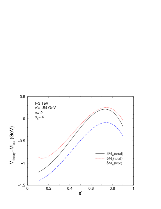
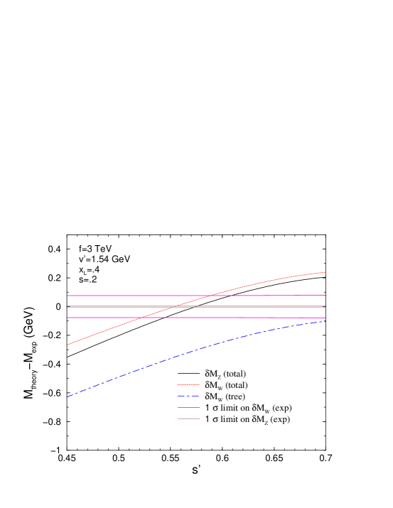
Figure 2: Prediction for $M_{W_{L}}$ as a function of the mixing angle $s^{\prime}$ at the tree level and the one-loop level. Also plotted is the correlation between $M_{Z}$ and $s^{\prime}$ for fixed $s$, $v^{\prime}$ and $f$. The cutoff scale $f$ in this plot is $3$ $TeV$, the $SU(2)$ triplet VEV $v^{\prime}=1.54\;GeV$, the mixing angle $s=0.2$, and $x_{L}=0.4$.

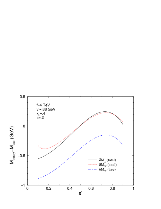
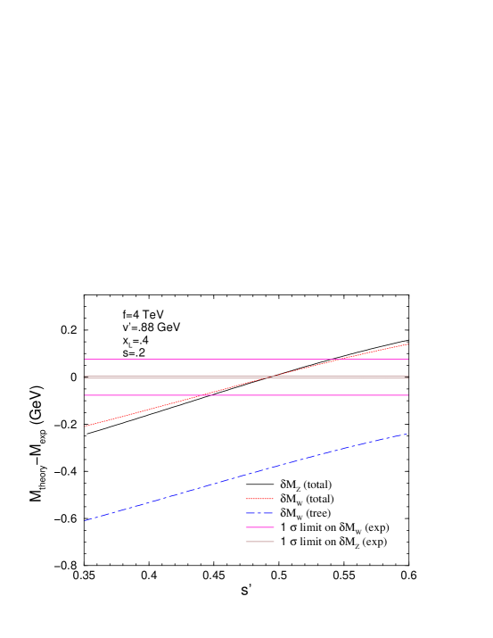
Figure 3: Prediction for $M_{W_{L}}$ as a function of the mixing angle $s^{\prime}$ at the tree level and the one-loop level. Also plotted is the correlation between $M_{Z}$ and $s^{\prime}$ for fixed $s$, $v^{\prime}$ and $f$. The cutoff scale $f$ in the plot is $4$ $TeV$, the $SU(2)$ triplet VEV $v^{\prime}=0.88\;GeV$, the mixing angle $s=0.2$, and $x_{L}=0.4$.

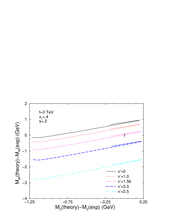
Figure 4: Parametric plot of $M_{W_{L}}-M_{Z}$ in terms of $s^{\prime}$ for different values of the $SU(2)$ triplet VEV, $v^{\prime}=0,\,1.0,\,1.56,\,2.0$ and $2.5$. The cutoff scale $f$ is $3$ $TeV$, the mixing angle $s=0.2$, and $x_{L}=0.4$. The data point with error bars on $M_{W_{L}}$ and $M_{Z}$ is also shown.

\psfrag{x_L}{\small$x_{L}$}\psfrag{s}{\small$s$}\psfrag{f=2TeV}{$\small f=2\,TeV$}\psfrag{f=3TeV}{$\small f=3\,TeV$}\psfrag{f=4TeV}{$\small f=4\,TeV$}\psfrag{f=5TeV}{$\small f=5\,TeV$}\psfrag{f=6TeV}{$\small f=6\,TeV$}\includegraphics[scale={0.32},angle={270}]{fig10.3.eps}

\psfrag{x_L}{\small$x_{L}$}\psfrag{s}{\small$s$}\psfrag{f=2TeV}{$\small f=2\,TeV$}\psfrag{f=3TeV}{$\small f=3\,TeV$}\psfrag{f=4TeV}{$\small f=4\,TeV$}\psfrag{f=5TeV}{$\small f=5\,TeV$}\psfrag{f=6TeV}{$\small f=6\,TeV$}\includegraphics[scale={0.32},angle={270}]{fig11.3.eps}

\psfrag{x_L}{\small$x_{L}$}\psfrag{s}{\small$s$}\psfrag{f=2TeV}{$\small f=2\,TeV$}\psfrag{f=3TeV}{$\small f=3\,TeV$}\psfrag{f=4TeV}{$\small f=4\,TeV$}\psfrag{f=5TeV}{$\small f=5\,TeV$}\psfrag{f=6TeV}{$\small f=6\,TeV$}\includegraphics[scale={0.32},angle={270}]{fig12.3.eps}

\psfrag{x_L}{\small$x_{L}$}\psfrag{s}{\small$s$}\psfrag{f=2TeV}{$\small f=2\,TeV$}\psfrag{f=3TeV}{$\small f=3\,TeV$}\psfrag{f=4TeV}{$\small f=4\,TeV$}\psfrag{f=5TeV}{$\small f=5\,TeV$}\psfrag{f=6TeV}{$\small f=6\,TeV$}\includegraphics[scale={0.32},angle={270}]{fig13.3.eps}

\psfrag{x_L}{\small$x_{L}$}\psfrag{s}{\small$s$}\psfrag{f=2TeV}{$\small f=2\,TeV$}\psfrag{f=3TeV}{$\small f=3\,TeV$}\psfrag{f=4TeV}{$\small f=4\,TeV$}\psfrag{f=5TeV}{$\small f=5\,TeV$}\psfrag{f=6TeV}{$\small f=6\,TeV$}\includegraphics[scale={0.32},angle={270}]{fig14.3.eps}

Figure 5: Allowed parameter space on the $(x_{L},s)$-plane, for $f=2,\;3,\;4,\;5,\;6$ TeV. The triplet VEV $v^{\prime}$ is allowed to vary between $0$ and the upper bound given by Eq. 33. For $f=(2,3,4,5,6)$ TeV, this bound is $v^{\prime}_{\mbox{\tiny max}}=(3.78,\,2.52,\,1.89,\,1.51,\,1.26)$ GeV.

\psfrag{v '}{\small$v^{\prime}$ (GeV)}\psfrag{s}{\small$s$}\psfrag{f=2TeV}{$\small f=2\,TeV$}\psfrag{f=3TeV}{$\small f=3\,TeV$}\psfrag{f=4TeV}{$\small f=4\,TeV$}\psfrag{f=5TeV}{$\small f=5\,TeV$}\psfrag{f=6TeV}{$\small f=6\,TeV$}\includegraphics[scale={0.32},angle={270}]{fig20.3.eps}

\psfrag{v '}{\small$v^{\prime}$ (GeV)}\psfrag{s}{\small$s$}\psfrag{f=2TeV}{$\small f=2\,TeV$}\psfrag{f=3TeV}{$\small f=3\,TeV$}\psfrag{f=4TeV}{$\small f=4\,TeV$}\psfrag{f=5TeV}{$\small f=5\,TeV$}\psfrag{f=6TeV}{$\small f=6\,TeV$}\includegraphics[scale={0.32},angle={270}]{fig21.3.eps}

\psfrag{v '}{\small$v^{\prime}$ (GeV)}\psfrag{s}{\small$s$}\psfrag{f=2TeV}{$\small f=2\,TeV$}\psfrag{f=3TeV}{$\small f=3\,TeV$}\psfrag{f=4TeV}{$\small f=4\,TeV$}\psfrag{f=5TeV}{$\small f=5\,TeV$}\psfrag{f=6TeV}{$\small f=6\,TeV$}\includegraphics[scale={0.32},angle={270}]{fig22.3.eps}

\psfrag{v '}{\small$v^{\prime}$ (GeV)}\psfrag{s}{\small$s$}\psfrag{f=2TeV}{$\small f=2\,TeV$}\psfrag{f=3TeV}{$\small f=3\,TeV$}\psfrag{f=4TeV}{$\small f=4\,TeV$}\psfrag{f=5TeV}{$\small f=5\,TeV$}\psfrag{f=6TeV}{$\small f=6\,TeV$}\includegraphics[scale={0.32},angle={270}]{fig23.3.eps}

\psfrag{v '}{\small$v^{\prime}$ (GeV)}\psfrag{s}{\small$s$}\psfrag{f=2TeV}{$\small f=2\,TeV$}\psfrag{f=3TeV}{$\small f=3\,TeV$}\psfrag{f=4TeV}{$\small f=4\,TeV$}\psfrag{f=5TeV}{$\small f=5\,TeV$}\psfrag{f=6TeV}{$\small f=6\,TeV$}\includegraphics[scale={0.32},angle={270}]{fig24.3.eps}

Figure 6: Allowed parameter space on the $(v^{\prime},s)$-plane for $f=2,\;3,\;4,\;5,\;6$ TeV. The mixing parameters $s^{\prime}$ and $x_{L}$ are allowed to vary between $0.01$ and $0.99$. For $f=(2,3,4,5,6)$ TeV, the upper bound given by Eq. 33 is $v^{\prime}_{\mbox{\tiny max}}=(3.78,\,2.52,\,1.89,\,1.51,\,1.26)$ GeV, respectively.

\psfrag{s '}{\small$s^{\prime}\;$}\psfrag{v '}{\small$v^{\prime}\qquad$}\includegraphics[scale={0.8},angle={270}]{fig3.3.eps}

Figure 7: Allowed parameter space on the $(v^{\prime},s^{\prime})$-plane for $f=2,\;3,\;4,\;5,\;6$ TeV. The mixing parameters $s$ and $x_{L}$ are allowed to vary between $0.01$ and $0.99$.

\psfrag{xL = 0.4}{\small$x_{L}=0.4$}\psfrag{s ' = 0.5}{\small$s^{\prime}=0.5$}\psfrag{s = 0.2}{\small$s=0.2$}\psfrag{v ' = 1 GeV}{\small$v^{\prime}=1GeV$}\psfrag{Dtree }{$\scriptstyle\Delta_{\mbox{\tiny tree}}\qquad\qquad$ }\psfrag{Df }{$\scriptstyle\Delta r_{Z}^{f}\qquad\qquad\qquad\;$}\psfrag{Ds }{$\scriptstyle\Delta r_{Z}^{S}\qquad\qquad\qquad\;$}\psfrag{D1loop }{$\scriptstyle\Delta\hat{r}_{Z}-\Delta_{\mbox{\tiny tree}}\qquad$}\psfrag{piww }{$\scriptstyle\Pi^{WW}(0)/M_{Z}^{2}\qquad$}\includegraphics[scale={0.8},angle={270}]{fig.nondecoupling.eps}

Figure 8: The tree level correction, $\Delta_{\mbox{\tiny tree}}$, the fermionic and scalar contributions to the one loop correction, $\Delta r_{Z}^{f}$ and $\Delta r_{Z}^{S}$, the total one loop correction, $\Delta\hat{r}-\Delta_{\mbox{\tiny tree}}$, and $\Pi^{WW}(0)/M_{Z}^{2}$ as functions of the cutoff scale $f$ at fixed $s$, $s^{\prime}$, $x_{L}$ and $v^{\prime}$.

V Conclusion

In this paper we considered the logarithmically enhanced one-loop radiative corrections to the $\rho$ parameter, due to the additional heavy fermions and SU(2) triplet Higgs, including the contributions from both fermion and scalar loops. We find the one-loop contributions, from both fermion and scalar sectors, can be comparable to the tree level correction to the $\rho$ parameter. In some cases, the one-loop contribution even dominates over the tree level correction due to the large logarithmic enhancement of the loop corrections arising from terms of ${\cal O}(\ln({f^{2}\over M_{Z}^{2}}))$.

The fermion loop contribution dominates in the low cutoff scale region. On the other hand, the scalar loop contribution dominates in the high cutoff scale $f$ region; it grows with the cutoff scale $f$. This in turn implies an upper bound on the cutoff scale. The non-decoupling of the $SU(2)$ triplet is due to the fact that $M_{\Phi}^{2}$ scales as $f^{2}$ when the parameters in the theory are fine-tuned to fix $v$ at the weak scale and the other parameters to be of order one. Without this fine-tuning, the triplet contributions do decouple for large $f$. This non-decoupling behavior of the scalar triplet will be further investigated in a future publication Chen and Dawson . Our results emphasize the need for a full one loop calculation.

Appendix A coupling constants in LLH Model

We summarize in this section the relevant coupling constants for our calculation Han et al. (2003). The gauge interaction of the fermions is given by

$$\mathcal{L} = i\overline{\psi}_{1}\gamma_{\mu}(g_{V}+g_{A}\gamma_{5})\psi_{2}X^{\mu}$$

$$= i\overline{\psi}_{1}\gamma_{\mu}(c_{L}P_{L}+c_{R}P_{R})\psi_{2}X^{\mu}\quad,$$

where $P_{L}=\frac{1}{2}(1-\gamma_{5})$ and $P_{R}=\frac{1}{2}(1+\gamma_{5})$ are the usual projection operators. The gauge coupling constants of the fermions are given in Table 2.

$X\overline{f}{f}$
$W_{L}\overline{t}b$:	$c_{L}=\frac{g}{\sqrt{2}}$	$c_{R}=0$
$W_{L}\overline{T}b$:	$c_{L}=-\frac{g}{\sqrt{2}}\frac{v}{f}x_{L}$	$c_{R}=0$
$Z_{L}\overline{t}t$:	$g_{V}=\frac{g}{2c_{W}}(\frac{1}{2}-\frac{4}{3}s_{W}^{2})$	$g_{A}=-\frac{g}{4c_{W}}$
$Z_{L}\overline{b}b$:	$g_{V}=\frac{g}{2c_{W}}(-1/2+\frac{2}{3}s_{W}^{2})$	$g_{A}=\frac{g}{4c_{W}}$
$Z_{L}\overline{T}T$:	$g_{V}=-\frac{2gs_{W}^{2}}{3c_{W}}$	$g_{A}=\mathcal{O}(v^{2}/f^{2})$
$Z_{L}\overline{T}t$:	$g_{V}=\frac{gx_{L}}{4c_{W}}\frac{v}{f}$	$g_{A}=-\frac{gx_{L}}{4c_{W}}\frac{v}{f}$
$A_{L}\overline{f}{f}$:	$g_{V}=eQ_{f}$	$g_{A}=0$

Table 2: Relevant coupling constants $X\overline{f}f$. As $M_{T}$ is of order $f$, gauge coupling constants for $T$ and $\overline{T}$ must be expanded to order $v/f$. For the coupling constants of the light fermions, we retain only the order $(v/f)^{0}$ terms. $Q_{f}$ is the electric charge of fermion $f$: $Q_{t}=Q_{T}=+2/3$, $Q_{b}=-1/3$. We make the approximation that $V_{tb}^{\mbox{\tiny SM}}=1$ Han et al. (2003).

The gauge coupling constants of the scalar fields are given in Table 3, 4 and 5. The parameters $s_{0}$, $s_{p}$ and $s_{+}$ describe the mixing in the neutral CP-even scalar, pseudoscalar and singly charged sectors, respectively. To leading order in $v^{\prime}\over v$ they are given by Han et al. (2003),

$$s_{0} \simeq 2\sqrt{2}\frac{v^{{}^{\prime}}}{v}$$ (76)

$$s_{p} = \frac{2\sqrt{2}v^{{}^{\prime}}}{\sqrt{v^{2}+8v^{{}^{\prime}2}}}\simeq 2\sqrt{2}\frac{v^{{}^{\prime}}}{v}$$ (77)

$$s_{+} = \frac{2v^{{}^{\prime}}}{\sqrt{v^{2}+4v^{{}^{\prime}2}}}\simeq 2\frac{v^{{}^{\prime}}}{v}\quad.$$ (78)

$XXSS$	$C_{\scriptstyle XXSS}$	$XXSS$	$C_{\scriptstyle XXSS}$
$W_{L}^{+}W_{L}^{-}HH$	$\frac{g^{2}}{2}$	$Z_{L}Z_{L}HH$	$\frac{g^{2}}{2c_{W}^{2}}$
$W_{L}^{+}W_{L}^{-}\Phi^{0}\Phi^{0}$	$g^{2}$	$Z_{L}Z_{L}\Phi^{0}\Phi^{0}$	$2\frac{g^{2}}{c_{W}^{2}}$
$W_{L}^{+}W_{L}^{-}\Phi^{P}\Phi^{P}$	$g^{2}$	$Z_{L}Z_{L}\Phi^{P}\Phi^{P}$	$2\frac{g^{2}}{c_{W}^{2}}$
$W_{L}^{+}W_{L}^{-}\Phi^{+}\Phi^{-}$	$2g^{2}$	$Z_{L}Z_{L}\Phi^{+}\Phi^{-}$	$2\frac{g^{2}}{c_{W}^{2}}s_{W}^{4}$
$W_{L}^{+}W_{L}^{-}\Phi^{++}\Phi^{--}$	$g^{2}$	$Z_{L}Z_{L}\Phi^{++}\Phi^{--}$	$2\frac{g^{2}}{c_{W}^{2}}(1-2s_{W}^{2})^{2}$
$A_{L}A_{L}\Phi^{+}\Phi^{-}$	$2e^{2}$	$A_{L}A_{L}\Phi^{++}\Phi^{--}$	$8e^{2}$
$A_{L}Z_{L}\Phi^{+}\Phi^{-}$	$-2e\frac{g}{c_{W}}s_{W}^{2}$	$A_{L}Z_{L}\Phi^{++}\Phi^{--}$	$4e\frac{g}{c_{W}}(1-2s_{W}^{2})$

Table 3: Relevant gauge coupling constants of the scalar fields, $C_{\scriptstyle XXSS}$ Han et al. (2003).

$XSS$	$C_{\scriptstyle XSS}$	$XSS$	$C_{\scriptstyle XSS}$	$XSS$	$C_{\scriptstyle XSS}$
$W_{L}^{+}H\Phi^{-}$	$-\frac{g}{2}(\sqrt{2}s_{0}-s_{+})$	$Z_{L}H\Phi^{P}$	$\frac{g}{2c_{W}}(s_{p}-2s_{0})$	$A_{L}\Phi^{+}\Phi^{-}$	$-e$
$W_{L}^{+}\Phi^{0}\Phi^{-}$	$-\frac{g}{\sqrt{2}}$	$Z_{L}\Phi^{0}\Phi^{P}$	$-\frac{g}{c_{W}}$	$A_{L}\Phi^{++}\Phi^{--}$	$-2e$
$W_{L}^{+}\Phi^{P}\Phi^{-}$	$\frac{g}{\sqrt{2}}$	$Z_{L}\Phi^{+}\Phi^{-}$	$\frac{g}{c_{W}}s_{W}^{2}$
$W_{L}^{+}\Phi^{+}\Phi^{--}$	$-g$	$Z_{L}\Phi^{++}\Phi^{--}$	$-\frac{g}{c_{W}}(1-2s_{W}^{2})$

Table 4: Relevant gauge coupling constants of the scalar fields, $C_{\scriptstyle XSS}$ Han et al. (2003).

$X_{1}X_{2}S$	$C_{X_{1}}C_{X_{2}}S$	$X_{1}X_{2}S$	$C_{X_{1}}C_{X_{2}}S$
$W_{L}^{+}W_{L}^{-}H$	$\frac{1}{2}g^{2}v$	$Z_{L}Z_{L}H$	$\frac{1}{2}\frac{g^{2}}{c_{W}^{2}}v$
$W_{L}^{+}W_{H}^{-}H$	$-\frac{1}{2}g^{2}\frac{c^{2}-s^{2}}{2sc}v$	$Z_{L}A_{H}H$	$-\frac{1}{2}\frac{gg^{{}^{\prime}}}{c_{W}}\frac{c^{{}^{\prime}2}-s^{{}^{\prime}2}}{2s^{{}^{\prime}}c^{{}^{\prime}}}v$
$W_{L}^{+}W_{L}^{-}\Phi^{0}$	$-\frac{1}{2}g^{2}(s_{0}v-2\sqrt{2}v^{{}^{\prime}})$	$Z_{L}Z_{L}\Phi^{0}$	$-\frac{1}{2}\frac{g^{2}}{c_{W}^{2}}(s_{0}v-4\sqrt{2}v^{{}^{\prime}})$
$W_{L}^{+}W_{H}^{-}\Phi^{0}$	$\frac{g^{2}}{4}\frac{c^{2}-s^{2}}{sc}(s_{0}v-2\sqrt{2}v^{\prime})$	$Z_{L}Z_{H}\Phi^{0}$	$\frac{1}{2}\frac{g^{2}}{c_{W}}\frac{c^{2}-s^{2}}{2sc}(s_{0}v-4\sqrt{2}v^{{}^{\prime}})$
$W_{L}^{+}A_{L}\Phi^{-}$	0	$Z_{L}Z_{H}H$	$-\frac{1}{2}\frac{g^{2}}{c_{W}}\frac{c^{2}-s^{2}}{2sc}v$
$W_{L}^{+}A_{H}\Phi^{-}$	$-\frac{1}{2}gg^{{}^{\prime}}\frac{c^{{}^{\prime}2}-s^{{}^{\prime}2}}{2s^{{}^{\prime}}c^{{}^{\prime}}}(s_{+}v-4v^{{}^{\prime}})$	$Z_{L}A_{H}\Phi^{0}$	$\frac{1}{2}\frac{gg^{{}^{\prime}}}{c_{W}}\frac{c^{{}^{\prime}2}-s^{{}^{\prime}2}}{2s^{{}^{\prime}}c^{{}^{\prime}}}(s_{0}v-4\sqrt{2}v^{{}^{\prime}})$
$W_{L}^{+}W_{L}^{+}\Phi^{--}$	$2g^{2}v^{{}^{\prime}}$	$W_{L}^{+}Z_{L}\Phi^{-}$	$-\frac{g^{2}}{c_{W}}v^{{}^{\prime}}$
$W_{L}^{+}W_{H}^{+}\Phi^{--}$	$-2g^{2}\frac{c^{2}-s^{2}}{2sc}v^{{}^{\prime}}$	$W_{L}^{+}Z_{H}\Phi^{-}$	$g^{2}\frac{c^{2}-s^{2}}{2sc}v^{{}^{\prime}}$
$W_{H}^{+}Z_{L}^{+}\Phi^{-}$	$\frac{g^{2}}{c_{w}}\frac{c^{2}-s^{2}}{2sc}v^{{}^{\prime}}$

Table 5: Relevant gauge coupling constants of the scalar fields, $C_{\scriptstyle XXS}$ Han et al. (2003).

Appendix B One-Loop Integrals

The one-loop integrals are decomposed in terms of Passarino-Veltman Passarino and Veltman (1979) functions which are defined in $n=4-2\epsilon$ dimensions,

$$Q^{4-n}\int\frac{d^{n}k}{(2\pi)^{n}}\frac{1}{k^{2}-m^{2}+i\epsilon} \equiv \frac{i}{16\pi^{2}}A_{0}(m^{2})$$ (79)

$$Q^{4-n}\int\frac{d^{n}k}{(2\pi)^{n}}\frac{1}{(k^{2}-m_{1}^{2}+i\epsilon)((k-p)^{2}-m_{2}^{2}+i\epsilon)} \equiv \frac{i}{16\pi^{2}}B_{0}(p^{2},m_{1}^{2},m_{2}^{2})$$ (80)

$$Q^{4-n}\int\frac{d^{n}k}{(2\pi)^{n}}\frac{k_{\mu}}{(k^{2}-m_{1}^{2}+i\epsilon)((k-p)^{2}-m_{2}^{2}+i\epsilon)} \equiv \frac{i}{16\pi^{2}}p_{\mu}B_{1}(p^{2},m_{1}^{2},m_{2}^{2})$$ (81)

$$Q^{4-n}\int\frac{d^{n}k}{(2\pi)^{n}}\frac{k_{\mu}k_{\nu}}{(k^{2}-m_{1}^{2}+i\epsilon)((k-p)^{2}-m_{2}^{2}+i\epsilon)} \equiv$$ (82)

$$\qquad\frac{i}{16\pi^{2}}[g_{\mu\nu}B_{22}(p^{2},m_{1}^{2},m_{2}^{2}) + p_{\mu}p_{\nu}B_{11}(p^{2},m_{1}^{2},m_{2}^{2})],$$

where ${1\over{\hat{\epsilon}}}\equiv{1\over\epsilon}(4\pi)^{\epsilon}\Gamma(1+\epsilon)$. We also define the following integrals,

$$I_{1}(a) = \int_{0}^{1}dx\;\ln[1-ax(1-x)]$$ (83)

$$I_{3}(a) = \int_{0}^{1}dx\;x(1-x)\ln[1-ax(1-x)]$$ (84)

$$I_{4}(a,b) = \int_{0}^{1}dx\;\ln[1-x+ax-bx(1-x)]$$ (85)

Appendix C One-Loop Contributions to Gauge Boson Self-Energies

The self-energies of the gauge bosons have the following structure

$$\Pi_{ij}(p^{2})=g_{\mu\nu}\;\Pi_{ij}^{T}(p^{2})+p_{\mu}p_{\nu}\;\Pi_{ij}^{L}(p^{2})\quad.$$ (86)

Only the coefficient of the $g_{\mu\nu}$ term, the transverse part of the self-energy, contributes to the mass renormalization of the gauge boson. We calculate the one-loop contributions to the gauge boson self-energies in unitary gauge, in which the contributions from the non-physical particles vanish. The fermion contribution to the gauge boson self-energy is gauge invariant and finite. Our calculation manifests these properties; this serves as a cross-check of our result. In the bosonic sector, the total contribution is gauge dependent and is Ultra-Violet-divergent Degrassi and Sirlin (1992). Nevertheless, one can show that the contribution which is logarithmically enhanced by $\ln(M_{\Phi}/m_{Z})$ is gauge independent, using Eq.(7)-(9) of Degrassi and Sirlin (1992).

C.1 Contributions of a fermion loop

The contribution due to the fermion loops to $\Pi^{XY}$, where $(XY)=\;(WW),\;(ZZ),\;(\gamma\gamma),\;(\gamma Z)$, is given by

$$\Pi^{XY}(p^{2}) = -\frac{1}{16\pi^{2}}\biggl{[}(c_{L}^{2}+c_{R}^{2})\biggl{(}2A_{0}(m_{2}^{2})+2m_{1}^{2}B_{0}(p^{2},m_{1}^{2},m_{2}^{2})$$

$$\quad-2p^{2}B_{1}(p^{2},m_{1}^{2},m_{2}^{2})-4B_{22}(p^{2},m_{1}^{2},m_{2}^{2})\biggr{)}$$

$$\quad-4c_{L}c_{R}m_{1}m_{2}B_{0}(p^{2},m_{1}^{2},m_{2}^{2})\biggr{]}\quad.$$

where $m_{1}$ and $m_{2}$ are the masses of the loop fermion doublets. At zero momentum transfer, this becomes,

$$\Pi^{XY}(0) = -\frac{1}{16\pi^{2}}\biggl{[}2(g_{V}^{2}+g_{A}^{2})\biggl{(}\frac{1}{2}(m_{1}^{2}+m_{2}^{2})+\frac{m_{1}^{4}}{m_{1}^{2}-m_{2}^{2}}\ln({Q^{2}\over m_{1}^{2}})-\frac{m_{2}^{4}}{m_{1}^{2}-m_{2}^{2}}\ln({Q^{2}\over m_{2}^{2}})\biggr{)}$$

$$\quad-4(g_{V}^{2}-g_{A}^{2})m_{1}m_{2}\biggl{(}1+\ln({Q^{2}\over m_{2}^{2}})+\frac{m_{1}^{2}}{m_{1}^{2}-m_{2}^{2}}\ln({m_{2}^{2}\over m_{1}^{2}})\biggr{)}\biggr{]}\quad.$$

Note that in the above expression the contribution proportional to $1/\hat{\epsilon}$ has been subtracted. We define the following shorthand notations

$$f_{1}(m_{1}^{2},m_{2}^{2}) = \frac{1}{2}(m_{1}^{2}+m_{2}^{2})+\frac{m_{1}^{4}}{m_{1}^{2}-m_{2}^{2}}\ln({Q^{2}\over m_{1}^{2}})-\frac{m_{2}^{4}}{m_{1}^{2}-m_{2}^{2}}\ln({Q^{2}\over m_{2}^{2}})$$ (89)

$$f_{2}(m_{1}^{2},m_{2}^{2}) = 1+\ln({Q^{2}\over m_{2}^{2}})+\frac{m_{1}^{2}}{m_{1}^{2}-m_{2}^{2}}\ln({m_{2}^{2}\over m_{1}^{2}})\quad.$$ (90)

C.2 Contributions of a pure scalar loop

The contribution of scalar loops with two vectors and two scalars ($VVSS$) has no momentum dependence, and is given by

$$\Pi^{XY}(p^{2})=\Pi^{XY}(0) = \frac{1}{16\pi^{2}}C_{\scriptstyle XYS_{1}S_{2}}A_{0}(m^{2})$$

$$= \frac{1}{16\pi^{2}}C_{\scriptstyle XYS_{1}S_{2}}m^{2}\biggl{[}1+\ln({Q^{2}\over m^{2}})+\frac{1}{\hat{\epsilon}}\biggr{]}\quad.$$

where $(XY)=(WW),\;(ZZ),\;(\gamma\gamma),\;(\gamma Z)$, and $m$ is the mass of the loop scalar fields. Note there is an extra symmetry factor $1/2$ if the particle in the loop is neutral. The contribution of the scalar loops with one vector and two scalars ($VSS$) is given by

$$\Pi^{XY}(p^{2})=-\frac{4}{16\pi^{2}}C_{\scriptstyle XS_{1}S_{2}}C_{\scriptstyle YS_{1}S_{2}}\;B_{22}(p^{2},m_{1}^{2},m_{2}^{2})$$ (92)

where $(XY)=(WW),\;(ZZ),\;(\gamma\gamma),\;(\gamma Z)$, and $m_{1}$ and $m_{2}$ are the masses of the loop scalar fields. For $p^{2}=0$,

$$\Pi^{XY}(0) = -\frac{4}{16\pi^{2}}C_{\scriptstyle XS_{1}S_{2}}C_{\scriptstyle YS_{1}S_{2}}\;\biggl{[}\,\frac{3}{8}(m_{1}^{2}+m_{2}^{2})+\frac{1}{4(m_{1}^{2}-m_{2}^{2})}\biggl{(}m_{1}^{4}\ln({Q^{2}\over m_{1}^{2}})-m_{2}^{4}\ln({Q^{2}\over m_{2}^{2}})\biggr{)}$$

$$\quad+\,\biggl{(}\frac{m_{1}^{2}+m_{2}^{2}}{4}\biggr{)}\frac{1}{\hat{\epsilon}}\,\biggr{]}\;.$$

We define the shorthand notation

$$g_{1}(m_{1}^{2},m_{2}^{2})=\frac{3}{8}(m_{1}^{2}+m_{2}^{2})+\frac{1}{4(m_{1}^{2}-m_{2}^{2})}\biggl{[}m_{1}^{4}\ln({Q^{2}\over m_{1}^{2}})-m_{2}^{4}\ln({Q^{2}\over m_{2}^{2}})\biggr{]}\quad.$$ (94)

In the limit $m_{1}^{2}=m_{2}^{2}=m^{2}$, this becomes

$$\Pi^{XY}(0)=-\frac{2}{16\pi^{2}}C_{\scriptstyle XS_{1}S_{2}}C_{\scriptstyle YS_{1}S_{2}}m^{2}\biggl{[}1+\ln({Q^{2}\over m^{2}})+\frac{1}{\hat{\epsilon}}\biggr{]}\quad.$$ (95)

C.3 Contributions of a gauge boson-scalar loop

The contribution of the gauge boson-scalar loops is given by

$$\Pi^{XX}(p^{2})=\frac{1}{16\pi^{2}}C_{\scriptstyle XX^{\prime}S}^{2}\biggl{[}B_{0}(p^{2},M_{X^{\prime}}^{2},m_{s}^{2})-\frac{1}{M_{X^{\prime}}^{2}}B_{22}(p^{2},M_{X^{\prime}}^{2},m_{s}^{2})\biggr{]}$$ (96)

where $(XY)=(WW),\;(ZZ)$, $M_{X^{\prime}}$ is the mass of the loop gauge boson $X^{\prime}$, and $m_{s}$ is the mass of the loop scalar field. For $p^{2}=0$,

$$\Pi^{XY}(0) = \frac{1}{16\pi^{2}}C_{\scriptstyle XX^{\prime}S}^{2}\biggl{[}\frac{5}{8}-\frac{3}{8}\frac{m_{s}^{2}}{M_{X^{\prime}}^{2}}+\frac{3}{4}(\frac{M_{X^{\prime}}^{2}}{M_{X^{\prime}}^{2}-m_{s}^{2}})\ln({Q^{2}\over M_{X^{\prime}}^{2}})$$

$$\quad+(\frac{m_{s}^{2}}{M_{X^{\prime}}^{2}-m_{s}^{2}})(-1+\frac{m_{s}^{2}}{4M_{X^{\prime}}^{2}})\ln({Q^{2}\over m_{s}^{2}})+(1-\frac{M_{X^{\prime}}^{2}+m_{s}^{2}}{4M_{X^{\prime}}^{2}})\frac{1}{\hat{\epsilon}}\,\biggr{]}$$

The contribution proportional to ${1\over 16\pi^{2}}\ln(m_{s}^{2})$ is gauge invariant,

$$g_{2}(m_{s}^{2},M_{X^{\prime}}^{2})\equiv\biggl{(}\frac{m_{s}^{2}}{M_{X^{\prime}}^{2}-m_{s}^{2}}\biggr{)}\biggl{[}(-1+\frac{m_{s}^{2}}{4M_{X^{\prime}}^{2}})\ln({Q^{2}\over m_{s}^{2}})\biggr{]}.$$ (98)

Appendix D Gauge boson self-energies in the LLH model

In our renormalization procedure, we need to calculate the following gauge boson self-energies, $\Pi^{\gamma\gamma\prime}(0)$, $\Pi^{\gamma Z}(0)$, $\Pi^{\gamma Z}(M_{Z}^{2})$, $\Pi^{WW}(0)$ and $\Pi^{ZZ}(M_{Z}^{2})$. Below we summarize the full results for diagrams due to fermion and scalar loops. In our numerical results, we keep only the contributions which are enhanced by large logarithms, $\ln(M^{2}/Q^{2})$, where $M$ is a heavy mass scale and $Q$ is typically the weak scale. The gauge independence in the bosonic sector can be retained by using the pinch technique or by using the background field formalism. This will be discussed in Chen and Dawson .

D.1 Contributions to $\Pi^{\gamma\gamma\prime}(0)$

There are five diagrams that contribute to $\Pi^{\gamma\gamma}(0)$ in the LLH model. These are loops having $(\overline{t}t)$, $(\overline{b}b)$, $(\overline{T}T)$, $(\Phi^{+}\Phi^{-})$, and $(\Phi^{++}\Phi^{--})$. The total contribution to $\Pi^{\gamma\gamma\prime}(0)$ in the LLH model is

$$\Pi^{\gamma\gamma\prime}(0)=\frac{\alpha}{4\pi}\biggl{[}\frac{5}{3}\ln\frac{Q^{2}}{M_{\Phi}^{2}}+\frac{16}{9}\ln\frac{Q^{2}}{m_{t}^{2}}+\frac{4}{9}\ln\frac{Q^{2}}{m_{b}^{2}}+\frac{16}{9}\ln\frac{Q^{2}}{m_{T}^{2}}+\frac{17}{3\hat{\epsilon}}\biggr{]}$$ (99)

D.2 Contributions to $\Pi^{\gamma Z}(p^{2})$

In the LLH model, there are six diagrams that contribute to $\Pi^{\gamma Z}(M_{Z}^{2})$. These are fermionic loops having $(\overline{t}t)$, $(\overline{T}T)$, the scalar loops due to $SSV$ couplings, $(\Phi^{+},\Phi^{-})$, $(\Phi^{++},\Phi^{--})$, and the $\Phi^{+}$ and $\Phi^{++}$ scalar loops due to $SSVV$ quartic couplings. The contributions to $\Pi^{\gamma Z}(M_{Z}^{2})$ due to the fermions are

$$\Pi^{\gamma Z}_{\scriptscriptstyle(\overline{t}t)}(M_{Z}^{2}) = \frac{2\alpha}{\pi s_{W}c_{W}}(\frac{1}{2}-\frac{4}{3}s_{W}^{2})M_{Z}^{2}\biggl{[}\frac{1}{3}\biggl{(}\ln\frac{Q^{2}}{m_{t}^{2}}+\frac{1}{\hat{\epsilon}})-2I_{3}(\frac{M_{Z}^{2}}{m_{t}^{2}}\biggr{)}\biggr{]}$$ (100)

$$\Pi^{\gamma Z}_{\scriptscriptstyle(\overline{T}T)}(M_{Z}^{2}) = -\frac{2\alpha}{\pi s_{W}c_{W}}(\frac{4s_{W}^{2}}{3})(\frac{1}{2}-\frac{4}{3}s_{W}^{2})M_{Z}^{2}$$

$$\qquad\cdot\biggl{[}\frac{1}{3}\biggl{(}\ln\frac{Q^{2}}{m_{T}^{2}}+\frac{1}{\hat{\epsilon}}\biggr{)}-2I_{3}(\frac{M_{Z}^{2}}{m_{T}^{2}})\biggr{]}$$

The sum of the contributions due to $SSV$ couplings is

$$\Pi^{\gamma Z}(M_{Z}^{2}) = \frac{\alpha}{2\pi}(\frac{s_{W}}{c_{W}})(5-\frac{2}{s_{W}^{2}})\biggl{[}\biggl{(}M_{\Phi}^{2}-\frac{1}{6}M_{Z}^{2}\biggr{)}\biggl{(}\ln\frac{Q^{2}}{M_{\Phi}^{2}}+\frac{1}{\hat{\epsilon}}\biggr{)}$$

$$\quad+\biggl{(}\frac{1}{6}M_{Z}^{2}-\frac{2}{3}M_{\Phi}^{2}\biggr{)}I_{1}\biggl{(}\frac{M_{Z}^{2}}{M_{\Phi}^{2}}\biggr{)}+M_{\Phi}^{2}-\frac{1}{9}M_{Z}^{2}\biggr{]}\;.$$

The sum of the contributions due to $SSVV$ couplings is

$$\Pi^{\gamma Z}(M_{Z}^{2})=-\frac{\alpha}{2\pi}\biggl{(}\frac{s_{W}}{c_{W}}\biggr{)}\biggl{(}5-\frac{2}{s_{W}^{2}}\biggr{)}\biggl{[}1+\ln\frac{Q^{2}}{M_{\Phi}^{2}}+\frac{1}{\hat{\epsilon}}\biggr{]}M_{\Phi}^{2}$$ (103)

The terms proportional to $M_{\Phi}^{2}$ and $M_{\Phi}^{2}\ln(Q^{2}/M_{\Phi}^{2})$ in Eq.(D.2) and (103) cancel among them-selves. The total contribution to $\Pi^{\gamma Z}(M_{Z}^{2})$ is thus given by, to order $\mathcal{O}(1/16\pi^{2})$,

$$\Pi^{\gamma Z}(M_{Z}^{2}) = \frac{2\alpha}{\pi s_{\theta}c_{\theta}}\biggl{(}\frac{1}{2}-\frac{4}{3}s_{\theta}^{2}\biggr{)}M_{Z}^{2}$$

$$\quad\cdot\biggl{[}\frac{1}{3}\ln(\frac{Q^{2}}{m_{t}^{2}})-2I_{3}(\frac{M_{Z}^{2}}{m_{t}^{2}})-\frac{4s_{\theta}^{2}}{3}\biggl{(}\frac{1}{3}\ln(\frac{Q^{2}}{M_{T}^{2}})-2I_{3}(\frac{M_{Z}^{2}}{M_{T}^{2}}\biggr{)}\biggl{]}$$

$$+\frac{\alpha s_{\theta}}{2\pi c_{\theta}}(5-\frac{2}{s_{\theta}^{2}})\biggl{[}-\frac{2}{3}M_{\Phi}^{2}I_{1}(\frac{M_{Z}^{2}}{M_{\Phi}^{2}})-\frac{1}{6}M_{Z}^{2}\biggl{(}\ln(\frac{Q^{2}}{M_{\Phi}^{2}})-I_{1}(\frac{M_{Z}^{2}}{M_{\Phi}^{2}})+\frac{2}{3}\biggr{)}\biggr{]}\;.$$

For $p^{2}=0$, it can be easily checked that the total fermionic contribution and the total scalar contribution to $\Pi^{\gamma Z}(0)$ vanish individually. Thus

$$\Pi^{\gamma Z}(0)=0,$$ (105)

as expected in the unitary gauge.

D.3 Contributions to $\Pi^{WW}(0)$

The full list of contributions of fermion loops to $\Pi^{WW}(0)$ is given as follows,

$$\Pi^{WW}_{(\overline{t}b)}(0) = -\frac{1}{16\pi^{2}}\frac{g^{2}}{2}f_{1}(m_{t}^{2},m_{b}^{2})$$

$$\Pi^{WW}_{(\overline{T}b)}(0) = -\frac{1}{16\pi^{2}}\frac{g^{2}}{2}(\frac{v}{f})^{2}x_{L}^{2}\,f_{1}(m_{T}^{2},m_{b}^{2})\quad.$$ (106)

The sum of the fermionic contributions to $\Pi^{WW}(0)$ is thus given by, to order $\mathcal{O}(1/16\pi^{2})$,

$$\Pi^{WW}_{f}(0) = -\frac{\alpha}{8\pi s_{\theta}^{2}}\biggl{[}f_{1}(m_{t}^{2},m_{b}^{2})+x_{L}^{2}(\frac{1}{\sqrt{2}G_{\mu}f^{2}})M_{T}^{2}\biggl{(}\frac{1}{2}+\frac{M_{T}^{2}}{M_{T}^{2}-m_{b}^{2}}\ln(\frac{Q^{2}}{M_{T}^{2}})\biggr{)}\;\biggr{]}.$$ (107)

where $M_{T}$ in the above equation is replaced by its leading order term, $M_{T}^{2}\rightarrow\frac{\sqrt{2}G_{\mu}m_{t}^{2}}{x_{L}(1-x_{L})}f^{2}$. The full list of contributions of scalar loops to $\Pi^{WW}(0)$ is given as follows,

$$\Pi^{WW}_{(s)}(0) = \frac{1}{16\pi^{2}}g^{2}\biggl{[}\frac{1}{4}m_{H}^{2}\biggl{(}1+ln(\frac{Q^{2}}{m_{H}^{2}})\biggr{)}+4M_{\Phi}^{2}\biggl{(}1+ln(\frac{Q^{2}}{M_{\Phi}^{2}})\biggr{)}\biggr{]}$$

$$\biggl{[}\mbox{\small s = sum of}\;{\scriptstyle h,\,\Phi^{0},\,\Phi^{P},\,\Phi^{+},\,\Phi^{++}}\biggr{]}$$

$$\Pi^{WW}_{(s_{1}s_{2})}(0) = -\frac{4}{16\pi^{2}}g^{2}\biggl{[}\frac{(\sqrt{2}s_{0}-s_{+})^{2}}{4}g_{1}(m_{H}^{2},M_{\Phi}^{2})+2g_{1}(M_{\Phi}^{2},M_{\Phi}^{2})\biggr{]}$$

$$= \frac{4}{16\pi^{2}}g^{2}\biggl{[}\frac{(\sqrt{2}s_{0}-s_{+})^{2}}{4}g_{1}(m_{H}^{2},M_{\Phi}^{2})+M_{\Phi}^{2}\biggl{(}1+ln(\frac{Q^{2}}{M_{\Phi}^{2}})\biggr{)}\biggr{]}$$

$$\qquad\biggl{[}{\scriptstyle(s_{1},s_{2})=\;\mbox{\small sum of}(H,\Phi^{-}),\,(\Phi^{0},\Phi^{-}),\,(\Phi^{P},\Phi^{-}),\,(\Phi^{+},\Phi^{--})\biggr{]}}\quad.$$

Note that the contribution of the triplet components $(\Phi^{0},\Phi^{P},\Phi^{+},\Phi^{++})$ to $\Pi^{WW}_{(s)}(0)$ cancels exactly the contribution of $(\Phi^{0},\Phi^{-}),\,(\Phi^{P},\Phi^{-}),\,(\Phi^{+},\Phi^{--})$ to $\Pi^{WW}_{(s_{1}s_{2})}(0)$. This prevents the appearance of contributions proportional to $M_{\Phi}^{2}$ and $M_{\Phi}^{2}ln(\frac{Q^{2}}{M_{\Phi}^{2}}).$ To order $\mathcal{O}(1/16\pi^{2})$, the sum of the contributions due to pure scalar loops is

$$\Pi^{WW}_{s}(0) = \frac{\alpha}{4\pi s_{\theta}^{2}}\biggl{[}\frac{1}{4}m_{H}^{2}\biggl{(}1+\ln(\frac{Q^{2}}{m_{H}^{2}})\biggr{)}$$ (111)

$$\quad-4\sqrt{2}G_{\mu}v^{\prime 2}M_{\Phi}^{2}\biggl{(}\frac{3}{8}+\frac{M_{\Phi}^{2}}{4(M_{\Phi}^{2}-m_{H}^{2})}\ln(\frac{Q^{2}}{M_{\Phi}^{2}})\biggr{)}\;\biggr{]}.$$

The complete list of contributions proportional to $\ln(m_{s}^{2})$ to $\Pi^{WW}(0)$ from scalar-gauge boson loops is,

$$\Pi^{WW}(0) = \frac{1}{16\pi^{2}}\;\{C_{{\scriptscriptstyle W_{L}W_{L}h}}^{2}g_{2}(m_{H}^{2},M_{W_{L}}^{2})+C_{\scriptscriptstyle W_{L}W_{H}h}^{2}g_{2}(m_{H}^{2},M_{W_{H}}^{2})$$ (112)

$$+C_{\scriptscriptstyle W_{L}W_{L}\Phi^{0}}^{2}g_{2}(M_{\Phi}^{2},M_{W_{L}}^{2})+C_{\scriptscriptstyle W_{L}W_{H}\Phi^{0}}^{2}g_{2}(M_{\Phi}^{2},M_{W_{H}}^{2})$$

$$+C_{\scriptscriptstyle W_{L}Z_{L}\Phi^{-}}^{2}g_{2}(M_{\Phi}^{2},M_{Z}^{2})+C_{\scriptscriptstyle W_{L}Z_{H}\Phi^{-}}^{2}g_{2}(M_{\Phi}^{2},M_{Z_{H}}^{2})$$

$$+C_{\scriptscriptstyle W_{L}A_{H}\Phi^{-}}^{2}g_{2}(M_{\Phi}^{2},M_{A_{H}}^{2})+C_{\scriptscriptstyle W_{L}W_{L}\Phi^{--}}^{2}g_{2}(M_{\Phi}^{2},M_{W_{L}}^{2})$$

$$+C_{\scriptscriptstyle W_{L}W_{H}\Phi^{--}}^{2}g_{2}(M_{\Phi}^{2},M_{W_{H}}^{2})\}$$

where the gauge coupling constants of the scalar fields are summarized in Table 5. To order $\mathcal{O}(1/16\pi^{2})$, the sum of the contributions due to scalar-gauge-boson loops is,

$$\Pi^{WW}_{sv}(0) = \frac{\alpha^{2}}{\sqrt{2}G_{\mu}s_{\theta}^{4}}\biggl{[}\frac{1}{4}\biggl{(}\frac{m_{H}^{2}}{M_{W_{L}}^{2}-m_{H}^{2}}\biggr{)}\biggl{(}-1+\frac{m_{H}^{2}}{M_{W_{L}}^{2}}\biggr{)}\ln(\frac{Q^{2}}{m_{H}^{2}})$$ (113)

$$\quad+\frac{\sqrt{2}G_{\mu}}{c_{\theta}^{2}}v^{\prime 2}\biggl{(}\frac{M_{\Phi}^{2}}{M_{Z}^{2}-M_{\Phi}^{2}}\biggr{)}\biggl{(}\frac{M_{\Phi}^{2}}{M_{Z}^{2}}\biggr{)}\ln(\frac{Q^{2}}{M_{\Phi}^{2}})$$

$$\quad+4\sqrt{2}G_{\mu}v^{\prime 2}\biggl{(}\frac{M_{\Phi}^{2}}{M_{W_{L}}^{2}-M_{\Phi}^{2}}\biggr{)}\biggl{(}\frac{M_{\Phi}^{2}}{M_{W_{L}}^{2}}\biggr{)}\ln(\frac{Q^{2}}{M_{\Phi}^{2}})\biggr{]}.$$

D.4 Contributions to $\Pi^{ZZ}(M_{Z}^{2})$

The complete list of fermionic contributions to the self-energy function $\Pi^{ZZ}(p^{2})$ are summarized below.

$$\Pi^{ZZ}_{\scriptscriptstyle(\overline{T}t)}(M_{Z}^{2}) = -\frac{1}{16\pi^{2}}(\frac{gx_{L}}{2c_{W}})^{2}\frac{v^{2}}{f^{2}}\biggl{[}-\frac{1}{3M_{Z}^{2}}(M_{T}^{2}-m_{t}^{2})^{2}+\frac{2}{9}M_{Z}^{2}$$

$$\quad+\frac{1}{6M_{Z}^{2}}\biggl{[}-M_{T}^{4}+m_{t}^{4}-2M_{Z}^{4}+M_{Z}^{2}\biggl{(}5M_{T}^{2}+m_{t}^{2}\biggr{)}\biggr{]}\ln\frac{Q^{2}}{M_{T}^{2}}$$

$$\quad+\frac{1}{6M_{Z}^{2}}\biggl{[}-m_{t}^{4}+M_{T}^{4}-2M_{Z}^{4}+M_{Z}^{2}\biggl{(}5m_{t}^{2}+M_{T}^{2}\biggr{)}\biggr{]}\ln\frac{Q^{2}}{m_{t}^{2}}$$

$$\quad-\frac{1}{6}\biggl{[}m_{t}^{2}+M_{T}^{2}-2M_{Z}^{2}+\frac{(m_{t}^{2}-M_{T}^{2})^{2}}{M_{Z}^{2}}\biggr{]}\biggl{(}I_{4}(\frac{M_{T}^{2}}{m_{t}^{2}},\frac{M_{Z}^{2}}{m_{t}^{2}})+I_{4}(\frac{M_{t}^{2}}{M_{T}^{2}},\frac{M_{Z}^{2}}{M_{T}^{2}})\biggr{)}$$

$$\quad+\frac{1}{\hat{\epsilon}}\biggl{[}M_{T}^{2}+m_{t}^{2}-\frac{2}{3}M_{Z}^{2}\biggr{]}\;\biggr{]}$$

$$\Pi^{ZZ}_{\scriptscriptstyle(\overline{t}T)}(M_{Z}^{2}) = \Pi^{ZZ}_{\scriptscriptstyle(\overline{T}t)}(M_{Z}^{2})$$ (115)

$$\Pi^{ZZ}_{\scriptscriptstyle(\overline{t}t)}(M_{Z}^{2}) = -\frac{1}{16\pi^{2}}(\frac{g}{2c_{W}})^{2}\biggl{[}2\biggl{(}(\frac{1}{2}-\frac{4}{3}s_{W}^{2})^{2}+\frac{1}{4}\biggr{)}h_{1}(m_{t}^{2})$$

$$\quad-\frac{16}{3}s_{W}^{2}(1-\frac{4}{3}s_{W}^{2})h_{2}(m_{t}^{2})$$

$$\quad+\frac{1}{\hat{\epsilon}}\biggl{[}2\biggl{(}\frac{1}{2}-\frac{4}{3}s_{W}^{2})^{2}+\frac{1}{4}\biggr{)}(2m_{t}^{2}-\frac{2}{3}M_{Z}^{2})+\frac{16}{3}s_{W}^{2}(1-\frac{4}{3}s_{W}^{2})m_{t}^{2}\biggr{]}\;\biggr{]}$$

$$\Pi^{ZZ}_{\scriptscriptstyle(\overline{b}b)}(M_{Z}^{2}) = -\frac{1}{16\pi^{2}}(\frac{g}{2c_{W}})^{2}\biggl{[}2\biggl{(}(\frac{1}{2}-\frac{2}{3}s_{W}^{2})^{2}+\frac{1}{4}\biggr{)}h_{1}(m_{b}^{2})$$

$$\quad-\frac{8}{3}s_{W}^{2}(1-\frac{2}{3}s_{W}^{2})h_{2}(m_{b}^{2})$$

$$\quad+\frac{1}{\hat{\epsilon}}\biggl{[}2\biggl{(}(\frac{1}{2}-\frac{2}{3}s_{W}^{2})^{2}+\frac{1}{4}\biggr{)}(2m_{b}^{2}-\frac{2}{3}M_{Z}^{2})+\frac{8}{3}s_{W}^{2}(1-\frac{2}{3}s_{W}^{2})m_{b}^{2}\biggr{]}\;\biggr{]}$$

$$\Pi^{ZZ}_{\scriptscriptstyle(\overline{T}T)}(M_{Z}^{2}) = -\frac{1}{16\pi^{2}}(\frac{2s_{W}^{2}g}{3c_{W}})^{2}\biggl{[}-\frac{4}{3}M_{Z}^{2}\biggl{(}\ln\frac{Q^{2}}{M_{T}^{2}}+\frac{1}{\hat{\epsilon}}\biggr{)}+\frac{4}{9}M_{Z}^{2}$$

$$\quad+\biggl{(}\frac{4}{3}M_{Z}^{2}+\frac{8}{3}M_{T}^{2}\biggr{)}I_{1}(\frac{M_{Z}^{2}}{M_{T}^{2}})\biggr{]}\;,$$

where $h_{1}(m^{2})$ and $h_{2}(m^{2})$ are defined as

$$h_{1}(m^{2}) = (2m^{2}-\frac{2}{3}M_{Z}^{2})\ln\frac{Q^{2}}{m^{2}}+\frac{2}{9}M_{Z}^{2}+\frac{2}{3}(M_{Z}^{2}-m^{2})I_{1}(\frac{M_{Z}^{2}}{m^{2}})$$ (119)

$$h_{2}(m^{2}) = m^{2}I_{1}(\frac{M_{Z}^{2}}{m^{2}})-m^{2}\ln\frac{Q^{2}}{m^{2}}\;.$$ (120)

To order $\mathcal{O}(1/16\pi^{2})$, the sum of the fermionic contributions to $\Pi^{ZZ}(M_{Z}^{2})$ is,

$$\Pi^{ZZ}_{f}(M_{Z}^{2}) = -\frac{\alpha}{8\pi s_{\theta}^{2}c_{\theta}^{2}}$$ (121)

$$\cdot\biggl{[}\quad(\frac{x_{L}^{2}}{\sqrt{2}G_{\mu}f^{2}})M_{T}^{2}\biggl{[}\frac{2m_{t}^{2}}{3M_{Z}^{2}}+\frac{5}{6}\ln(\frac{Q^{2}}{M_{T}^{2}})+\frac{1}{6}\ln(\frac{Q^{2}}{m_{t}^{2}})$$

$$\qquad\qquad-\frac{1}{6}\biggl{(}1-\frac{2m_{t}^{2}}{M_{Z}^{2}}\biggr{)}\biggl{(}I_{4}(\frac{M_{T}^{2}}{m_{t}^{2}},\frac{M_{Z}^{2}}{m_{t}^{2}})+I_{4}(\frac{m_{t}^{2}}{M_{T}^{2}},\frac{M_{Z}^{2}}{M_{T}^{2}})\biggr{)}\;\biggr{]}$$

$$\qquad-(\frac{x_{L}^{2}}{3\sqrt{2}G_{\mu}f^{2}})\biggl{(}1+\frac{\Delta s_{\theta}^{2}}{c_{\theta}^{2}}-\frac{\Delta s_{\theta}^{2}}{s_{\theta}^{2}}-\frac{1}{4\sqrt{2}G_{\mu}f^{2}}-4\frac{v^{\prime 2}}{f^{2}}\biggr{)}\frac{M_{T}^{4}}{M_{Z}^{2}}\biggl{[}1$$

$$\qquad\qquad+\frac{1}{2}\biggl{(}\ln(\frac{m_{t}^{2}}{M_{T}^{2}})+I_{4}(\frac{M_{T}^{2}}{m_{t}^{2}},\frac{M_{Z}^{2}}{m_{t}^{2}})+I_{4}(\frac{m_{t}^{2}}{M_{T}^{2}},\frac{M_{Z}^{2}}{M_{T}^{2}})\biggr{)}\biggr{]}$$

$$\qquad+\biggl{(}(\frac{1}{2}-\frac{4}{3}s_{\theta}^{2})^{2}+\frac{1}{4}\biggr{)}h_{1}(m_{t}^{2})-\frac{8}{3}s_{\theta}^{2}(1-\frac{4}{3}s_{\theta}^{2})h_{2}(m_{t}^{2})$$

$$\qquad+\biggl{(}(\frac{1}{2}-\frac{2}{3}s_{\theta}^{2})^{2}+\frac{1}{4}\biggr{)}h_{1}(m_{b}^{2})-\frac{4}{3}s_{\theta}^{2}(1-\frac{2}{3}s_{\theta}^{2})h_{2}(m_{b}^{2})$$

$$\qquad+\frac{8}{9}s_{\theta}^{4}M_{Z}^{2}\biggl{[}-\frac{4}{3}\ln(\frac{Q^{2}}{M_{T}^{2}})+\frac{4}{9}+\frac{4}{3}I_{1}(\frac{M_{Z}^{2}}{M_{T}^{2}})\biggr{]}\quad\biggr{]}$$

The sum of the scalar contributions due to VVSS quartic couplings is

$$\Pi^{ZZ}_{(s)}(M_{Z}^{2}) = \frac{1}{16\pi^{2}}\frac{g^{2}}{c_{W}^{2}}\biggl{[}\frac{1}{4}m_{H}^{2}\biggl{(}1+\ln(\frac{Q^{2}}{m_{H}^{2}})\biggr{)}$$

$$+2\biggl{(}1+s_{W}^{4}+(1-2s_{W}^{2})^{2}\biggr{)}M_{\Phi}^{2}\biggl{(}1+\ln(\frac{Q^{2}}{M_{\Phi}^{2}})\biggr{)}\;\biggr{]}$$

$$\biggl{[}\mbox{\small s = sum of}\;{\scriptstyle h,\,\Phi^{0},\,\Phi^{P},\,\Phi^{+},\,\Phi^{++}}\biggr{]}\;.$$

The sum of scalar contributions due to $(\Phi^{0}\Phi^{P})$, $(\Phi^{+}\Phi^{-})$ and $(\Phi^{++}\Phi^{--})$ loops, is given by,

$$\Pi^{ZZ}_{(s_{1}s_{2})}(M_{Z}^{2}) = -\frac{1}{16\pi^{2}}(\frac{2g^{2}}{3c_{W}^{2}})\biggl{(}1+s_{W}^{4}+(1-2s_{W}^{2})^{2}\biggr{)}\biggl{[}3M_{\Phi}^{2}-\frac{1}{3}M_{Z}^{2}$$

$$\qquad+\biggl{(}3M_{\Phi}^{2}-\frac{1}{2}M_{Z}^{2}\biggr{)}\biggl{(}\ln\frac{Q^{2}}{M_{\Phi}^{2}}+\frac{1}{\hat{\epsilon}}\biggr{)}+\biggl{(}\frac{1}{2}M_{Z}^{2}-2M_{\Phi}^{2}\biggr{)}I_{1}(\frac{M_{Z}^{2}}{M_{\Phi}^{2}})\;\biggr{]}.$$

The contributions proportional to $M_{\Phi}^{2}$ and $M_{\Phi}^{2}\ln\frac{Q^{2}}{M_{\Phi}^{2}}$ due to VVSS quartic couplings cancel exactly those due to VSS couplings. Thus there is no contribution proportional to $M_{\Phi}^{2}$ and $M_{\Phi}^{2}\ln(\frac{Q^{2}}{M_{\Phi}^{2}})$ due to pure scalar loops. For the contribution due to $(H\Phi^{P})$ loop, we have

$$\Pi^{ZZ}_{(H\Phi^{P})}(M_{Z}^{2}) = -\frac{1}{16\pi^{2}}(\frac{g}{c_{W}})^{2}(s_{p}-2s_{0})^{2}\frac{1}{12}$$ (124)

$$\quad\cdot\biggl{[}\frac{1}{2}\biggl{(}3M_{\Phi}^{2}+3m_{H}^{2}-M_{Z}^{2}\biggr{)}\biggl{(}\frac{1}{\hat{\epsilon}}+\ln(\frac{Q^{4}}{M_{\Phi}^{2}m_{H}^{2}})\biggr{)}$$

$$\qquad+\frac{1}{2M_{Z}^{2}}\biggl{(}M_{\Phi}^{4}-m_{H}^{4}+M_{Z}^{2}(M_{\Phi}^{2}-m_{H}^{2})\biggr{)}\ln(\frac{M_{\Phi}^{2}}{m_{H}^{2}})$$

$$\qquad+\frac{1}{2M_{Z}^{2}}\biggl{(}M_{\Phi}^{4}+(m_{H}^{2}-M_{Z}^{2})^{2}-2M_{\Phi}^{2}(m_{H}^{2}+M_{Z}^{2})\;\biggr{)}$$

$$\qquad\qquad\qquad\cdot\biggl{(}I_{4}(\frac{m_{H}^{2}}{M_{\Phi}^{2}},\frac{M_{Z}^{2}}{M_{\Phi}^{2}})+I_{4}(\frac{M_{\Phi}^{2}}{m_{H}^{2}},\frac{M_{\Phi}^{2}}{m_{H}^{2}})\biggr{)}$$

$$\qquad+\frac{1}{3M_{Z}^{2}}\biggl{(}3M_{\Phi}^{4}+M_{\Phi}^{2}(9M_{Z}^{2}-6m_{H}^{2})+3m_{H}^{4}$$

$$\qquad\qquad\qquad\qquad-2M_{Z}^{4}+9m_{H}^{2}M_{Z}^{2}\biggr{)}\;\biggr{]}\;.\quad$$

In terms of the input parameters, the sum of the contributions to $\Pi^{ZZ}(M_{Z}^{2})$ due to pure scalar loop to $\mathcal{O}(1/16\pi^{2})$ is,

$$\Pi^{ZZ}_{s}(M_{Z}^{2}) = \frac{\alpha}{4\pi s_{\theta}^{2}c_{\theta}^{2}}\biggl{[}\frac{1}{4}m_{H}^{2}\biggl{(}1+\ln(\frac{Q^{2}}{m_{H}^{2}})\biggr{)}$$ (125)

$$\qquad+\biggl{(}1+s_{\theta}^{4}+(1-2s_{\theta}^{2})^{2}\biggr{)}\biggl{[}\frac{2}{3}M_{Z}^{2}\biggl{(}\frac{1}{3}+\frac{1}{2}\ln(\frac{Q^{2}}{M_{\Phi}^{2}})-\frac{1}{2}I_{1}\biggl{(}\frac{M_{Z}^{2}}{M_{\Phi}^{2}}\biggr{)}\,\biggl{)}+\frac{4}{3}M_{\Phi}^{2}I_{1}(\frac{M_{Z}^{2}}{M_{\Phi}^{2}})\biggr{]}$$

$$\qquad-\frac{\sqrt{2}G_{\mu}v^{\prime 2}}{12}M_{\Phi}^{2}\biggl{[}\frac{3}{2}\ln(\frac{Q^{4}}{m_{H}^{2}M_{\Phi}^{2}})+\frac{1}{2}\ln(\frac{M_{\Phi}^{2}}{m_{H}^{2}})+\biggl{(}3-\frac{2m_{H}^{2}}{M_{Z}^{2}}\biggr{)}$$

$$\qquad\qquad\qquad-\frac{m_{H}^{2}}{M_{Z}^{2}}\biggl{(}I_{4}(\frac{m_{H}^{2}}{M_{\Phi}^{2}},\frac{M_{Z}^{2}}{M_{\Phi}^{2}})+I_{4}(\frac{M_{\Phi}^{2}}{m_{H}^{2}},\frac{M_{Z}^{2}}{m_{H}^{2}})\biggr{)}\biggr{]}$$

$$\qquad-\frac{\sqrt{2}G_{\mu}v^{\prime 2}}{24}\biggl{(}1-\frac{\Delta s_{\theta}^{2}}{s_{\theta}^{2}}+\frac{\Delta s_{\theta}^{2}}{c_{\theta}^{2}}-\frac{1}{4\sqrt{2}G_{\mu}f^{2}}-\frac{4v^{\prime 2}}{f^{2}}\biggr{)}\frac{M_{\Phi}^{4}}{M_{Z}^{2}}$$

$$\qquad\qquad\qquad\cdot\biggl{[}2+\ln(\frac{M_{\Phi}^{2}}{m_{H}^{2}})+I_{4}(\frac{m_{H}^{2}}{M_{\Phi}^{2}},\frac{M_{Z}^{2}}{M_{\Phi}^{2}})+I_{4}(\frac{M_{\Phi}^{2}}{m_{H}^{2}},\frac{M_{Z}^{2}}{m_{H}^{2}})\biggr{]}\;\biggr{]}.$$

The contributions to $\Pi^{ZZ}(M_{Z}^{2})$ due to scalar-gauge-boson loops have the following form

$$\Pi^{ZZ}_{\scriptscriptstyle(VS)}(M_{Z}^{2}) = \frac{1}{16\pi^{2}}C_{XX^{\prime}S}^{2}$$

$$\quad\cdot\biggl{[}\;\biggl{(}1-\frac{1}{12M_{X^{\prime}}^{2}}\biggl{(}3M_{X^{\prime}}^{2}+3m_{S}^{2}-M_{Z}^{2}\biggr{)}\,\biggr{)}\biggl{(}\frac{1}{2}\ln\biggl{(}\frac{Q^{4}}{M_{X^{\prime}}^{2}m_{S}^{2}}\biggr{)}+\frac{1}{\hat{\epsilon}}\biggr{)}$$

$$\qquad-\biggl{(}\frac{1}{2}+\frac{1}{24M_{Z}^{2}M_{X^{\prime}}^{2}}\biggl{(}M_{X^{\prime}}^{4}+(m_{S}^{2}-M_{Z}^{2})^{2}-2M_{X^{\prime}}^{2}\biggl{(}m_{S}^{2}+M_{Z}^{2}\biggr{)}\;\biggr{)}\;\biggr{)}$$

$$\qquad\qquad\cdot\biggl{(}I_{4}\biggl{(}\frac{m_{S}^{2}}{M_{X^{\prime}}^{2}},\frac{M_{Z}^{2}}{M_{X^{\prime}}^{2}}\biggr{)}+I_{4}\biggl{(}\frac{M_{X^{\prime}}^{2}}{m_{S}^{2}},\frac{M_{Z}^{2}}{m_{s}^{2}}\biggr{)}\,\biggr{)}$$

$$\qquad-\frac{1}{24M_{Z}^{2}M_{X^{\prime}}^{2}}\biggl{(}M_{X^{\prime}}^{4}-m_{S}^{4}+M_{Z}^{2}(M_{X^{\prime}}^{2}-m_{S}^{2})\biggr{)}\ln\biggl{(}\frac{M_{X^{\prime}}^{2}}{m_{S}^{2}}\biggr{)}$$

$$\qquad-\frac{1}{36M_{Z}^{2}M_{X^{\prime}}^{2}}\biggl{(}3M_{X^{\prime}}^{4}+M_{X^{\prime}}^{2}(9M_{Z}^{2}-6m_{S}^{2})+3m_{S}^{4}-2M_{Z}^{4}+9m_{S}^{2}M_{Z}^{2}\biggr{)}\;\biggr{]}\;.$$

where $M_{X^{\prime}}$ is the mass of the loop gauge boson and $m_{S}$ is the mass of the loop scalar field. The contribution proportional to $\ln(m_{s}^{2})/16\pi^{2}$ is

$$g_{3}(m_{s}^{2},M_{X^{\prime}}^{2}) \equiv \frac{1}{2}\biggl{[}1-\frac{1}{12M_{X^{\prime}}^{2}}\biggl{(}3m_{s}^{4}+3M_{X^{\prime}}^{2}-M_{Z}^{2}\biggr{)}\;\biggr{]}\ln(\frac{Q^{2}}{m_{s}^{2}})\;.$$ (127)

Using this notation, the total contribution to $\Pi^{ZZ}(M_{Z}^{2})$ proportional to $\ln(m_{s}^{2})$ from scalar-gauge boson loops, is

$$\Pi^{ZZ}_{\scriptscriptstyle(VS)}(M_{Z}^{2}) = \frac{1}{16\pi^{2}}\;\biggl{[}C_{{\scriptscriptstyle Z_{L}Z_{L}h}}^{2}g_{3}(m_{H}^{2},M_{Z}^{2})+C_{\scriptscriptstyle Z_{L}A_{H}h}^{2}g_{3}(m_{H}^{2},M_{A_{H}}^{2})$$

$$+C_{\scriptscriptstyle Z_{L}Z_{L}\Phi^{0}}^{2}g_{3}(M_{\Phi}^{2},M_{Z}^{2})+C_{\scriptscriptstyle Z_{L}Z_{H}\Phi^{0}}^{2}g_{3}(M_{\Phi}^{2},M_{Z_{H}}^{2})$$

$$+C_{\scriptscriptstyle Z_{L}Z_{H}H}^{2}g_{3}(m_{H}^{2},M_{Z_{H}}^{2})+C_{\scriptscriptstyle Z_{L}A_{H}\Phi^{0}}^{2}g_{3}(M_{\Phi}^{2},M_{A_{H}}^{2})$$

$$+C_{\scriptscriptstyle Z_{L}W_{L}\Phi^{-}}^{2}g_{3}(M_{\Phi}^{2},M_{W_{L}}^{2})+C_{\scriptscriptstyle Z_{L}W_{H}\Phi^{-}}^{2}g_{3}(M_{\Phi}^{2},M_{W_{H}}^{2})\biggr{]}$$

where the gauge coupling constants of the scalar fields are summarized in Table 5. Expanding the coupling constants and masses in terms of the input parameters, to $\mathcal{O}(1/16\pi^{2})$, $\Pi^{ZZ}_{\scriptscriptstyle(VS)}(M_{Z}^{2})$ is given by

$$\Pi^{ZZ}_{\scriptscriptstyle(VS)}(M_{Z}^{2}) = \frac{\alpha^{2}}{8\sqrt{2}G_{\mu}s_{\theta}^{4}c_{\theta}^{4}}$$

$$\cdot\biggl{[}\quad\biggl{(}\frac{5}{6}-\frac{m_{H}^{2}}{4M_{Z}^{2}}+\frac{3(c^{\prime 2}-s^{\prime 2})^{2}}{16s^{\prime 2}c^{\prime 2}}+\frac{3(c^{2}-s^{2})^{2}}{16s^{2}c^{2}}\;\biggr{)}\ln\biggl{(}\frac{Q^{2}}{m_{H}^{2}}\biggr{)}$$

$$\qquad+\biggl{[}\;8\sqrt{2}G_{\mu}v^{\prime 2}\biggl{(}\frac{5}{6}-\frac{M_{\Phi}^{2}}{4M_{Z}^{2}}\biggr{)}$$

$$\qquad\qquad+\frac{(c^{2}-s^{2})^{2}}{4s^{2}c^{2}}\biggl{(}\frac{3}{4}-\frac{M_{\Phi}^{2}}{4M_{Z_{H}}^{2}}\biggr{)}$$

$$\qquad\qquad+\frac{\sqrt{2}G_{\mu}(c^{\prime 2}-s^{\prime 2})^{2}v^{\prime 2}}{4s^{\prime 2}c^{\prime 2}}\biggl{(}\frac{3}{4}-\frac{M_{\Phi}^{2}}{4M_{A_{H}}^{2}}\biggr{)}\;\biggr{]}\ln\biggl{(}\frac{Q^{2}}{M_{\Phi}^{2}}\biggr{)}\;\biggr{]}$$

Figure 9: Complete list of diagrams due to fermions and scalar fields to the self-energy of the photon, $A_{L}$.

Figure 10: Complete list of diagrams due to fermions and scalar fields to the self-energy $\Pi^{\gamma Z}$.

Figure 11: Complete list of diagrams due to fermions and scalar fields to the self-energy of the Standard Model W gauge boson.

Figure 12: Complete list of diagrams due to fermions and scalar fields to the self-energy of the Standard Model Z gauge boson.

References

- lep (2003) LEP Electroweak Working Group, http://lepewwg.web.cern.ch/LEPEWWG.
- Arkani-Hamed et al. (2002a) N. Arkani-Hamed, A. G. Cohen, E. Katz, and A. E. Nelson, JHEP 07, 034 (2002a), eprint hep-ph/0206021.
- Arkani-Hamed et al. (2001) N. Arkani-Hamed, A. G. Cohen, and H. Georgi, Phys. Lett. B513, 232 (2001), eprint hep-ph/0105239.
- Arkani-Hamed et al. (2002b) N. Arkani-Hamed, A. G. Cohen, T. Gregoire, and J. G. Wacker, JHEP 08, 020 (2002b), eprint hep-ph/0202089.
- Arkani-Hamed et al. (2002c) N. Arkani-Hamed et al., JHEP 08, 021 (2002c), eprint hep-ph/0206020.
- Low et al. (2002) I. Low, W. Skiba, and D. Smith, Phys. Rev. D66, 072001 (2002), eprint hep-ph/0207243.
- Kaplan and Schmaltz (2003) D. E. Kaplan and M. Schmaltz, eprint hep-ph/0302049.
- Chang and Wacker (2003) S. Chang and J. G. Wacker, eprint hep-ph/0303001.
- Skiba and Terning (2003) W. Skiba and J. Terning, eprint hep-ph/0305302.
- Chang (2003) S. Chang, eprint hep-ph/0306034.
- Dimopoulos and Preskill (1982) S. Dimopoulos and J. Preskill, Nucl. Phys. B199, 206 (1982).
- Kaplan and Georgi (1984) D. B. Kaplan and H. Georgi, Phys. Lett. B136, 183 (1984).
- Kaplan et al. (1984) D. B. Kaplan, H. Georgi, and S. Dimopoulos, Phys. Lett. B136, 187 (1984).
- Georgi and Kaplan (1984) H. Georgi and D. B. Kaplan, Phys. Lett. B145, 216 (1984).
- Georgi et al. (1984) H. Georgi, D. B. Kaplan, and P. Galison, Phys. Lett. B143, 152 (1984).
- Dugan et al. (1985) M. J. Dugan, H. Georgi, and D. B. Kaplan, Nucl. Phys. B254, 299 (1985).
- Banks (1984) T. Banks, Nucl. Phys. B243, 125 (1984).
- Csaki et al. (2003a) C. Csaki, J. Hubisz, G. D. Kribs, P. Meade, and J. Terning, Phys. Rev. D67, 115002 (2003a), eprint hep-ph/0211124.
- Hewett et al. (2002) J. L. Hewett, F. J. Petriello, and T. G. Rizzo, JHEP 10, 062 (2003b), eprint hep-ph/0211218.
- Csaki et al. (2003b) C. Csaki, J. Hubisz, G. D. Kribs, P. Meade, and J. Terning, Phys. Rev. D68, 035009 (2003b), eprint hep-ph/0303236.
- Kribs (2003) G. Kribs, eprint hep-ph/0305157.
- Gregoire et al. (2003) T. Gregoire, D. R. Smith, and J. G. Wacker, eprint hep-ph/0305275.
- Perelstein et al (2003) M. Perelstein, M. E. Peskin, and A. Pierce, eprint hep-ph/0310039.
- Casalbuoni et al (2003) R. Casalbuoni, A. Deandrea and M. Oertel, eprint hep-ph/0311038.
- Kilian and Reuter (2003) W. Kilian and J. Reuter, eprint hep-ph/0311095.
- Han et al. (2003) T. Han, H. E. Logan, B. McElrath, and L.-T. Wang, Phys. Rev. D67, 095004 (2003), eprint hep-ph/0301040.
- Passarino (1990) G. Passarino, Nucl. Phys. B361, 351 (1991).
- Lynn (1990) B. W. Lynn, Nucl. Phys. B381, 467 (1992).
- Blank and Hollik (1998) T. Blank and W. Hollik, Nucl. Phys. B514, 113 (1998), eprint hep-ph/9703392.
- Czakon et al (1999) M. Czakon, M. Zralek and J. Gluza, Nucl. Phys. B573, 57 (2000).
- Czakon et al (1999) M. Czakon, J. Gluza, F. Jegerlehner and M. Zralek, Eur. Phys. J. C13, 275 (2000).
- Book (2002) Particle Data Book, K. Hagiwara et al, Phys. Rev. D66, 010001 (2002), URL http://pdg.lbl.gov.
- Chanowitz et al. (1978) M. S. Chanowitz, M. A. Furman, and I. Hinchliffe, Phys. Lett. B78, 285 (1978).
- Mahajan (2003) N. Mahajan, eprint hep-ph/0310098.
- Toussaint (1978) D. Toussain, Phys. Rev. D18, 1626 (1978).
- Senjanovic and Sokorac (1978) G. Senjanovic and A. Sokorac, Phys. Rev. D18, 2708 (1978).
- (37) M.-C. Chen and S. Dawson, under preparation.
- Passarino and Veltman (1979) G. Passarino and M. J. G. Veltman, Nucl. Phys. B160, 151 (1979).
- Degrassi and Sirlin (1992) G. Degrassi and A. Sirlin, Nucl. Phys. B383, 73 (1992).