Light pseudoscalar mesons in a nonlocal SU(3) chiral quark model

Abstract

We study the properties of the light pseudoscalar mesons in a three flavor chiral quark model with nonlocal separable interactions. We concentrate on the evaluation of meson masses and decay constants, considering both the cases of Gaussian and Lorentzian nonlocal regulators. The results are found to be in quite good agreement with the empirical values, in particular in the case of the ratio $f_{K}/f_{\pi}$ and the anomalous decay $\pi^{0}\to\gamma\gamma$. In addition, the model leads to a reasonable description of the observed phenomenology in the $\eta-\eta^{\prime}$ sector, even though it implies the existence of two significantly different state mixing angles.

I Introduction

The properties of the light pseudoscalar mesons (i.e. the pions, kaons and etas) provide a suitable ground for the study of the basic nonperturbative features of Quantum Chromodynamics (QCD). As well known, the QCD Lagrangian shows an approximate $U(3)_{L}\otimes U(3)_{R}$ chiral symmetry, which is spontaneously broken down to $U(3)_{V}$ in the low momentum, nonperturbative regime. The fact that, instead of nine, only eight pseudoscalar quasi-Goldstone bosons are observed in Nature is usually explained in terms of the so-called $U(1)_{A}$ anomaly. This anomaly is again related to nonperturbative aspects of QCD, and it is believed to be mainly responsible for the rather large $\eta^{\prime}$ mass. Unfortunately, so far it has not been possible to obtain detailed information about the properties of the light pseudoscalar mesons directly from QCD, and most of the present theoretical work on the subject relies in low energy effective theories. Among them the Nambu-Jona-Lasinio (NJL) model NJL61 and its three flavor extensions KH88 ; BJM87 ; TTKK90 ; KLVW90 are some of the most popular ones. In the NJL model the quark fields interact via local effective vertices which are subject to chiral symmetry. If such interaction is strong enough chiral symmetry is spontaneously broken and pseudoscalar Goldstone bosons appear reports . As an improvement of the local NJL scheme, some covariant nonlocal extensions have been studied in the last few years Rip97 . Nonlocality arises naturally in the context of several quite successful approaches to low-energy quark dynamics as, for example, the instanton liquid model SS98 and the Schwinger-Dyson resummation techniques RW94 . It has been also argued that nonlocal covariant extensions of the NJL model have several advantages over the local scheme. Indeed, nonlocal interactions regularize the model in such a way that anomalies are preserved AS99 and charges properly quantized, the effective interaction is finite to all orders in the loop expansion and there is not need to introduce extra cut-offs, soft regulators such as Gaussian functions lead to small next-to-leading order corrections Rip00 , etc. In addition, it has been shown BB95 ; PB98 that a proper choice of the nonlocal regulator and the model parameters can lead to some form of quark confinement, in the sense that the effective quark propagator has no poles at real energies.

Until now, most of the research work on nonlocal chiral models has been restricted to the flavor $SU(2)$ sector including applications to the baryonic sector BGR02 ; RWB03 and to the study of the phase transitions at finite temperature and densities GDS01 . The aim of the present paper is to extend this type of models so as to include strange degrees of freedom, and to analyze the predictions for the masses and decay constants for the pions, kaons and the $\eta-\eta^{\prime}$ system.

This article is organized as follows. In Sec. II we present the general formalism and derive the expressions needed to evaluate the different meson properties. The numerical results for some specific nonlocal regulators together with the corresponding discussions are given in Sec. III, while in Sec. IV we present our conclusions. Finally, we include an Appendix with some details concerning the evaluation of quark loop integrals.

II The formalism

II.1 Effective action

We start by the Euclidean quark effective action

$$S_{E} = \int d^{4}x\ \left\{\bar{\psi}(x)\left[-i\gamma_{\mu}\partial_{\mu}+\hat{m}_{c}\right]\psi(x)-\frac{G}{2}\left[j_{a}^{S}(x)\ j_{a}^{S}(x)+j_{a}^{P}(x)\ j_{a}^{P}(x)\right]\right.$$ (1)

$$\qquad\qquad\left.-\frac{H}{4}A_{abc}\left[j_{a}^{S}(x)j_{b}^{S}(x)j_{c}^{S}(x)-3\ j_{a}^{S}(x)j_{b}^{P}(x)j_{c}^{P}(x)\right]\right\}\;,$$

where $\psi$ is a chiral $U(3)$ vector that includes the light quark fields, $\psi\equiv(u\;d\;s)^{T}$, while $\hat{m}_{c}={\rm diag}(m_{u},m_{d},m_{s})$ is the current quark mass matrix. We will work from now on in the isospin symmetry limit, in which $m_{u}=m_{d}$. The currents $j_{a}^{S,P}(x)$ are given by

$$j_{a}^{S}(x) = \int d^{4}y\ d^{4}z\ r(y-x)\ r(x-z)\ \bar{\psi}(y)\ \lambda_{a}\ \psi(z)\,,$$ (2)

$$j_{a}^{P}(x) = \int d^{4}y\ d^{4}z\ r(y-x)\ r(x-z)\ \bar{\psi}(y)\ i\gamma_{5}\ \lambda_{a}\ \psi(z)\,,$$ (3)

where the regulator $r(x-y)$ is local in momentum space, namely

$$r(x-y)=\int\frac{d^{4}p}{(2\pi)^{4}}\ e^{-i(x-y)p}\ r(p)\;,$$ (4)

and the matrices $\lambda_{a}$, with $a=0,..,8$, are the usual eight Gell-Mann $3\times 3$ matrices —generators of $SU(3)$— plus $\lambda_{0}=\sqrt{2/3}\;\openone_{3\times 3}$. Finally, the constants $A_{abc}$ are defined by

$$A_{abc}=\frac{1}{3!}\ \epsilon_{ijk}\ \epsilon_{mnl}\ \left(\lambda_{a}\right)_{im}\left(\lambda_{b}\right)_{jn}\left(\lambda_{c}\right)_{kl}\;.$$ (5)

The corresponding partition function $Z=\int{\cal D}\bar{\psi}\,{\cal D}\psi\,\exp[-S_{E}]$ can be bosonized in the usual way introducing the scalar and pseudoscalar meson fields $\sigma_{a}(x)$ and $\pi_{a}(x)$ respectively, together with auxiliary fields $S_{a}(x)$ and $P_{a}(x)$. Integrating out the quark fields we get

$$Z = \int{\cal D}\sigma_{a}\,{\cal D}\pi_{a}\ \det A\int{\cal D}S_{a}\,{\cal D}P_{a}\ \exp\left[\int d^{4}x\;(\sigma_{a}S_{a}+\pi_{a}P_{a})\right]\times$$ (6)

$$\exp\left\{\int d^{4}x\left[\frac{G}{2}\left(S_{a}S_{a}+P_{a}P_{a}\right)+\frac{H}{4}A_{abc}\left(S_{a}S_{b}S_{c}-3S_{a}P_{b}P_{c}\right)\right]\right\}\;,$$

where the operator $A$ reads, in momentum space,

$$A(p,p^{\prime})=(\,-\hbox to0.0pt{/\hss}p+\hat{m}_{c})\,(2\pi)^{4}\,\delta^{(4)}(p-p^{\prime})+r(p)\,\left[\sigma_{a}(p-p^{\prime})+i\gamma_{5}\ \pi_{a}(p-p^{\prime})\right]\lambda_{a}\ r(p^{\prime})\;.$$ (7)

To perform the integration over the fields $S_{a}$ and $P_{a}$ we use the Stationary Phase Approximation (SPA). This means to replace the integral over $S_{a}$ and $P_{a}$ by the integrand evaluated at its minimizing values $\tilde{S}_{a}(\sigma_{b}(x),\pi_{c}(x))$ and $\tilde{P}_{a}(\sigma_{b}(x),\pi_{c}(x))$. The latter are required to satisfy

$$\sigma_{a}+G\tilde{S}_{a}+\frac{3H}{4}\ A_{abc}\left[\tilde{S}_{b}\ \tilde{S}_{c}-\tilde{P}_{b}\ \tilde{P}_{c}\right]=0\;,$$

$$\pi_{a}+G\tilde{P}_{a}-\frac{3H}{2}\ A_{abc}\ \tilde{S}_{b}\ \tilde{P}_{c}=0\;.$$ (8)

Thus, within the SPA the bosonized effective action reads

$$S_{E}=-\,\ln\,{\rm det}\,A-\int d^{4}x\ \bigg{[}\sigma_{a}\tilde{S}_{a}+\pi_{a}\tilde{P}_{a}+\frac{G}{2}\left(\tilde{S}_{a}\tilde{S}_{a}+\tilde{P}_{a}\tilde{P}_{a}\right)+\frac{H}{4}A_{abc}\left(\tilde{S}_{a}\tilde{S}_{b}\tilde{S}_{c}-3\,\tilde{S}_{a}\tilde{P}_{b}\tilde{P}_{c}\right)\bigg{]}\;.$$ (9)

At this stage we assume that the $\sigma_{a}$ fields can have nontrivial translational invariant mean field values $\bar{\sigma}_{a}$ while the pseudoscalar field cannot. Thus, we write

$$\sigma_{a}(x) = \bar{\sigma}_{a}+\delta\sigma_{a}(x)\;,$$

$$\pi_{a}(x) = \delta\pi_{a}(x)\;.$$ (10)

Note that due to charge conservation only $\bar{\sigma}_{a=0,3,8}$ can be different from zero. Moreover, $\sigma_{3}$ also vanishes in the isospin limit. After replacing Eqs. (10) in the bosonized effective action (9) and expanding up to second order in the fluctuations $\delta\sigma_{a}(x)$ and $\delta\pi_{a}(x)$ we get

$$S_{E}=S_{E}^{MFA}+S_{E}^{quad}+\ \dots$$ (11)

Here the mean field action reads

$$\frac{S_{E}^{MFA}}{V^{(4)}}=-\,2\,N_{c}\int\frac{d^{4}p}{(2\pi)^{4}}\ {\rm Tr}\,\ln\left[p^{2}\,\openone_{3\times 3}+\Sigma^{2}(p)\right]-\frac{1}{2}\left[\sum_{i}\left(\bar{\sigma}_{i}\bar{S}_{i}+\frac{G}{2}\bar{S}_{i}\bar{S}_{i}\right)+\frac{H}{2}\bar{S}_{u}\bar{S}_{d}\bar{S}_{s}\right]\;,$$ (12)

where for convenience we have changed to a new basis in which $S_{i}$, with $i=u,d,s$ (or equivalently $i=1,2,3$) are given by

$$S_{u} = \sqrt{\frac{2}{3}}\,S_{0}+S_{3}+\frac{1}{\sqrt{3}}\,S_{8}\;,\quad S_{d}=\sqrt{\frac{2}{3}}\,S_{0}-S_{3}+\frac{1}{\sqrt{3}}\,S_{8}\;,\quad S_{s}=\sqrt{\frac{2}{3}}\,S_{0}+\frac{2}{\sqrt{3}}\,S_{8}\;,$$

and similar definitions hold for $\bar{\sigma}_{i}$ in terms of $\bar{\sigma}_{0}$, $\bar{\sigma}_{3}$ and $\bar{\sigma}_{8}$. In Eq. (12) we have also defined $\Sigma(p)={\rm diag}(\Sigma_{u}(p),\Sigma_{d}(p),\Sigma_{s}(p))$, with $\Sigma_{i}(p)=m_{i}+\bar{\sigma}_{i}\,r^{2}(p)$, whereas the mean field values $\bar{S}_{i}$ are given by $\bar{S}_{i}=\tilde{S}_{i}(\bar{\sigma}_{j},0)$. Note that in the isospin limit $\bar{\sigma}_{u}=\bar{\sigma}_{d}$, thus we have $\Sigma_{u}(p)=\Sigma_{d}(p)$.

In order to deal with the mesonic degrees of freedom, we also introduce a more convenient basis defined by

$$\phi_{ij}=\frac{1}{\sqrt{2}}\,\left(\lambda_{a}\phi_{a}\right)_{ij}\;,$$ (13)

where $\phi=\sigma,\pi$, and the indices $i,j$ run from 1 to 3. For the pseudoscalar fields one has in this way

$$\delta\pi_{ij}=\left(\begin{array}[]{ccc}\displaystyle\frac{\pi^{0}}{\sqrt{2}}+\frac{\eta_{8}}{\sqrt{6}}+\frac{\eta_{0}}{\sqrt{3}}&\pi^{+}&K^{+}\\ \pi^{-}&\displaystyle-\frac{\pi^{0}}{\sqrt{2}}+\frac{\eta_{8}}{\sqrt{6}}+\frac{\eta_{0}}{\sqrt{3}}&K^{0}\\ K^{-}&\bar{K}^{0}&\displaystyle-\frac{2\,\eta_{8}}{\sqrt{6}}+\frac{\eta_{0}}{\sqrt{3}}\end{array}\right)_{ij}.$$ (14)

The second piece of the effective action in Eq. (11) —quadratic in the meson fluctuations— can be written now as

$$S_{E}^{quad}=\frac{1}{2}\int\frac{d^{4}p}{(2\pi)^{4}}\left[G^{+}_{ij,kl}(p)\ \delta\sigma_{ij}(p)\ \delta\sigma_{kl}(-p)+G^{-}_{ij,kl}(p)\ \delta\pi_{ij}(p)\;\delta\pi_{kl}(-p)\right]\;,$$ (15)

where we have defined

$$G^{\pm}_{ij,kl}(p)=C^{\pm}_{ij}(p)\ \delta_{il}\,\delta_{jk}+\left((r^{\pm})^{-1}\right)_{ij,kl}\;,$$ (16)

with

$$C^{\pm}_{ij}(p^{2}) = -\,8\,N_{c}\int\frac{d^{4}q}{(2\pi)^{4}}\ \frac{r^{2}(q^{+})r^{2}(q^{-})\left[(q^{+}\cdot q^{-})\mp\Sigma_{i}(q^{+})\Sigma_{j}(q^{-})\right]}{\left[(q^{+})^{2}+\Sigma_{i}^{2}(q^{+})\right]\left[(q^{-})^{2}+\Sigma_{j}^{2}(q^{-})\right]}\;,\qquad q^{\pm}=q\pm p/2\;,$$ (17)

$$r^{\pm}_{ij,kl} = G\ \delta_{il}\,\delta_{jk}\pm\frac{H}{2}\ \epsilon_{ikn}\,\epsilon_{jln}\ \bar{S}_{n}\;.$$ (18)

II.2 Mean field approximation and chiral condensates

The mean field values $\bar{\sigma}_{u}$ and $\bar{\sigma}_{s}$ can be found by minimizing the action $S_{E}^{MFA}$. Taking into account Eqs. (8), a straightforward exercise leads to the following set of coupled “gap equations”:

$$\left\{\begin{array}[]{rcl}\displaystyle\bar{\sigma}_{u}+G\,\bar{S}_{u}+\frac{H}{2}\,\bar{S}_{u}\bar{S}_{s}&=&0\\ \displaystyle\bar{\sigma}_{s}+G\,\bar{S}_{s}+\frac{H}{2}\,\bar{S}_{u}^{2}&=&0\ \ ,\end{array}\right.$$ (19)

where

$$\bar{S}_{i}=-\,8\,N_{c}\int\frac{d^{4}p}{(2\pi)^{4}}\ \frac{\Sigma_{i}(p)\ r^{2}(p)}{p^{2}+\Sigma_{i}^{2}(p)}\;.$$ (20)

The chiral condensates are given by the vacuum expectation values $\langle\,\bar{u}u\,\rangle=\langle\,\bar{d}d\,\rangle$ and $\langle\,\bar{s}s\,\rangle$. They can be easily obtained by performing the variation of $Z^{MFA}=\exp[-S_{E}^{MFA}]$ with respect to the corresponding current quark masses. For $q=u,s$ one obtains

$$\langle\,\bar{q}q\,\rangle=-\,4\,N_{c}\int\frac{d^{4}p}{(2\pi)^{4}}\ \frac{\Sigma_{q}(p)}{p^{2}+\Sigma_{q}^{2}(p)}\;.$$ (21)

II.3 Meson masses and quark-meson coupling constants

From the quadratic effective action $S_{E}^{quad}$ it is possible to derive the scalar and pseudoscalar meson masses as well as the quark-meson couplings. In what follows we will consider explicitly only the case of pseudoscalar mesons. The corresponding expressions for the scalar sector are completely equivalent, just replacing the upper indices “$-$” by “$+$”. In terms of physical fields, the contribution of the pseudoscalar mesons to $S_{E}^{quad}$ can be written as

$$\left.S_{E}^{quad}\right|_{P} = \frac{1}{2}\int\frac{d^{4}p}{(2\pi)^{4}}\,\bigg{\{}G_{\pi}(p^{2})\left[\pi^{0}(p)\ \pi^{0}(-p)+2\,\pi^{+}(p)\ \pi^{-}(-p)\right]$$ (22)

$$\qquad\qquad+G_{K}(p^{2})\left[2\,K^{0}(p)\ \bar{K}^{0}(-p)+2\,K^{+}(p)\ K^{-}(-p)\right]$$

$$\qquad\qquad+G_{\eta}(p^{2})\ \eta(p)\ \eta(-p)+G_{\eta^{\prime}}(p^{2})\ \eta^{\prime}(p)\ \eta^{\prime}(-p)\bigg{\}}\;.$$

Here, the fields $\eta$ and $\eta^{\prime}$ are related to the $U(3)_{V}$ states $\eta_{0}$ and $\eta_{8}$ according to

$$\eta = \cos\theta_{\eta}\ \eta_{8}-\sin\theta_{\eta}\ \eta_{0}$$ (23)

$$\eta^{\prime} = \sin\theta_{\eta^{\prime}}\ \eta_{8}+\cos\theta_{\eta^{\prime}}\ \eta_{0}\ ,$$ (24)

where the mixing angles $\theta_{\eta,\eta^{\prime}}$ are defined in such a way that there is no $\eta-\eta^{\prime}$ mixing at the level of the quadratic action. The functions $G_{P}(p^{2})$ introduced in Eq. (22) are given by

$$G_{\pi}(p^{2}) = \left[(G+\frac{H}{2}\bar{S}_{s})^{-1}+C^{-}_{uu}(p^{2})\right]$$ (25)

$$G_{K}(p^{2}) = \left[(G+\frac{H}{2}\bar{S}_{u})^{-1}+C^{-}_{us}(p^{2})\right]$$ (26)

$$G_{\eta}(p^{2}) = \frac{G^{-}_{88}(p^{2})+G^{-}_{00}(p^{2})}{2}-\sqrt{\left[G^{-}_{08}(p^{2})\right]^{2}\!+\!\left[\frac{G^{-}_{88}(p^{2})-G^{-}_{00}(p^{2})}{2}\right]^{2}}$$ (27)

$$G_{\eta^{\prime}}(p^{2}) = \frac{G^{-}_{88}(p^{2})+G^{-}_{00}(p^{2})}{2}+\sqrt{\left[G^{-}_{08}(p^{2})\right]^{2}\!+\!\left[\frac{G^{-}_{88}(p^{2})-G^{-}_{00}(p^{2})}{2}\right]^{2}}\;,$$ (28)

where

$$G^{-}_{88}(p^{2}) = \frac{1}{3}\left[\frac{6G-4H\bar{S}_{u}-2H\bar{S}_{s}}{2G^{2}-GH\bar{S}_{s}-H^{2}\bar{S}_{u}^{2}}+C^{-}_{uu}(p^{2})+2\,C^{-}_{ss}(p^{2})\right]$$

$$G^{-}_{08}(p^{2}) = \frac{\sqrt{2}}{3}\left[\frac{H(\bar{S}_{s}-\bar{S}_{u})}{2G^{2}-GH\bar{S}_{s}-H^{2}\bar{S}_{u}^{2}}+C^{-}_{uu}(p^{2})-C^{-}_{ss}(p^{2})\right]$$

$$G^{-}_{00}(p^{2}) = \frac{1}{3}\left[\frac{6G+4H\bar{S}_{u}-H\bar{S}_{s}}{2G^{2}-GH\bar{S}_{s}-H^{2}\bar{S}_{u}^{2}}+2\,C^{-}_{uu}(p^{2})+C^{-}_{ss}(p^{2})\right]\,.$$ (29)

The meson masses are obtained by solving the equations

$$G_{P}(-m_{P}^{2})=0\;,$$ (30)

with $P=\pi$, $K$, $\eta$ and $\eta^{\prime}$, while the $\eta$ and $\eta^{\prime}$ mixing angles, which are in general different from each other, are given by

$$\mbox{tan}\ 2\,\theta_{\eta,\eta^{\prime}} = \frac{2\,G^{-}_{08}(p^{2})}{G^{-}_{00}(p^{2})-G^{-}_{88}(p^{2})}\Big{|}_{p^{2}=-m^{2}_{\eta,\eta^{\prime}}}\;.$$ (31)

Now the meson fields have to be renormalized, so that the residues of the corresponding propagators at the meson poles are set equal to one. This means that one should define renormalized fields $\tilde{\phi}(p)=Z^{-1/2}_{\phi}\ \phi(p)$ such that, close to the poles, the quadratic effective lagrangian reads

$$\left.{\cal L}_{E}^{quad}\right|_{\phi}=\frac{1}{2}\left(p^{2}+m^{2}_{\phi}\right)\ \tilde{\phi}(p)\ \tilde{\phi}(-p)\;.$$ (32)

In this way, the wave function renormalization constants $Z_{P}$ are given by

$$Z_{P}^{-1}=\frac{dG_{P}(p^{2})}{dp^{2}}\bigg{|}_{p^{2}=-m_{P}^{2}}\;,$$ (33)

with $P=\pi$, $K$, $\eta$ and $\eta^{\prime}$. Finally, the meson-quark coupling constants $G_{Pq}$ are given by the original residues of the meson propagators at the corresponding poles,

$$G_{Pq}=Z^{1/2}_{P}\;.$$ (34)

II.4 Weak decay constants of pseudoscalar mesons

By definition, the pseudoscalar meson weak decay constants are given by the matrix elements of the axial currents $A^{a}_{\mu}(x)$ between the vacuum and the renormalized one-meson states at the meson pole:

$$\langle\,0|A^{a}_{\mu}(0)|\tilde{\phi}_{b}(p)\,\rangle=i\;f_{ab}\;p_{\mu}\;.$$ (35)

For $a,b=1\dots 7$, the constants $f_{ab}$ can be written as $\delta_{ab}\,f_{\phi}$, with $\phi=\pi$ for $a=1,2,3$ and $\phi=K$ for $a=4$ to 7. In contrast, as occurs with the mass matrix, the decay constants become mixed in the $a=0,8$ sector.

In order to obtain the expression for the axial current, one has to gauge the effective action $S_{E}$ by introducing a set of axial gauge fields ${\cal A}^{a}_{\mu}$. For a local theory, this gauging procedure can be done simply by performing the replacement

$$\partial_{\mu}\rightarrow\partial_{\mu}+\frac{i}{2}\;\gamma_{5}\;\lambda_{a}\;{\cal A}^{a}_{\mu}(x)\;.$$ (36)

However, since in the present case we are dealing with nonlocal fields, an extra replacement has to be performed in the regulator $r(x-y)$ BB95 ; PB98 ; BKB91 . One has

$$r(x-y)\rightarrow\mbox{P}\exp\left[\frac{i}{2}\int_{x}^{y}ds_{\mu}\ \gamma_{5}\ \lambda_{a}\ {\cal A}^{a}_{\mu}(s)\right]r(x-y)\;,$$ (37)

where $s$ represents an arbitrary path that connects $x$ with $y$. In the present work we will use the so-called “straight line path”, which means

$$s_{\mu}=x_{\mu}+\alpha\left(y_{\mu}-x_{\mu}\right)\;,$$ (38)

with $0\leq\alpha\leq 1$. Once the gauged effective action is obtained, it is straightforward to get the axial current as the derivative of such action with respect to ${\cal A}^{a}_{\mu}(x)$ evaluated at ${\cal A}^{a}_{\mu}(x)=0$. Then, performing the derivative of the resulting expressions with respect to the renormalized meson fields, one can finally identify the corresponding meson weak decay constants. After a rather lengthy calculation, we find that the pion and kaon decay constants are given by

$$f_{\pi} = 4\,f_{uu}(-m_{\pi}^{2})\ Z_{\pi}^{1/2}\;,$$ (39)

$$f_{K} = 2\left[f_{us}(-m_{K}^{2})+f_{su}(-m_{K}^{2})\right]Z_{K}^{1/2}\;,$$ (40)

where

$$f_{ij}(p^{2}) = 2\,N_{c}\int\frac{d^{4}q}{(2\pi)^{4}}\left.\ \frac{(p\cdot q_{\alpha}^{+})}{p^{2}}\ \frac{r(q_{\alpha}^{+})r(q_{\alpha}^{-})\Sigma_{j}(q_{\alpha}^{-})}{\left[(q_{\alpha}^{+})^{2}+\Sigma_{i}^{2}(q_{\alpha}^{+})\right]\left[(q_{\alpha}^{-})^{2}+\Sigma_{j}^{2}(q_{\alpha}^{-})\right]}\;\right|_{\alpha=1/2}$$ (41)

$$+\;4\,N_{c}\int\frac{d^{4}q}{(2\pi)^{4}}\ \frac{(p\cdot q)}{p^{2}}\ \frac{dr(q)}{dq^{2}}\,\int_{0}^{1}d\alpha\ \frac{1}{(q^{+}_{\alpha})^{2}+\Sigma_{i}^{2}(q^{+}_{\alpha})}$$

$$\times\ \bigg{\{}r(q^{-}_{\alpha})\;[\Sigma_{i}(q^{+}_{\alpha})-m_{i}]\ \frac{\left[(q^{+}_{\alpha}\cdot q^{-}_{\alpha})+\Sigma_{i}(q^{+}_{\alpha})\Sigma_{j}(q^{-}_{\alpha})\right]}{(q^{-}_{\alpha})^{2}+\Sigma_{j}^{2}(q^{-}_{\alpha})}+\;r(q^{+}_{\alpha})\;\Sigma_{i}(q^{+}_{\alpha})\bigg{\}}\;,$$

with

$$q^{+}_{\alpha} = q+(1-\alpha)\ p\;,$$

$$q^{-}_{\alpha} = q-\alpha\ p\ .$$ (42)

In the case of the $\eta-\eta^{\prime}$ system, two decays constants can be defined for each component $a=0,8$ of the axial current PDG02 . They can be written in terms of the $f_{ab}$ decay constants and the previously defined mixing angles $\theta_{\eta,\eta^{\prime}}$ as

$$f^{a}_{\eta} = \left[f_{a8}(-m_{\eta}^{2})\cos\theta_{\eta}-f_{a0}(-m_{\eta}^{2})\sin\theta_{\eta}\right]\ Z_{\eta}^{1/2}$$ (43)

$$f^{a}_{\eta^{\prime}} = \left[f_{a8}(-m_{\eta^{\prime}}^{2})\sin\theta_{\eta^{\prime}}+f_{a0}(-m_{\eta^{\prime}}^{2})\cos\theta_{\eta^{\prime}}\right]\ Z_{\eta^{\prime}}^{1/2}\;.$$ (44)

Within our model, the decay constants $f_{ab}$ for $a,b=0,8$ are related to the $f_{ij}$ defined in Eq. (41) by

$$f_{88}(p^{2}) = \frac{4}{3}\left[2f_{ss}(p^{2})+f_{uu}(p^{2})\right]$$ (45)

$$f_{00}(p^{2}) = \frac{4}{3}\left[2f_{uu}(p^{2})+f_{ss}(p^{2})\right]$$ (46)

$$f_{08}(p^{2})=f_{80}(p^{2}) = \frac{4\sqrt{2}}{3}\left[f_{uu}(p^{2})-f_{ss}(p^{2})\right]\;.$$ (47)

It is clear that both the nondiagonal decay constants $f_{08}$, $f_{80}$ as well as the mixing angles $\theta_{\eta}$ and $\theta_{\eta^{\prime}}$ vanish in the $SU(3)$ symmetry limit.

II.5 Anomalous $P\to\gamma\gamma$ decays

To go further with the analysis of light pseudoscalar meson decays, let us evaluate the anomalous decays of $\pi^{0}$, $\eta$ and $\eta^{\prime}$ into two photons. In general, the corresponding amplitudes can be written as

$$A(P\to\gamma\gamma)\ =\ e^{2}\;g_{P\gamma\gamma}\ \epsilon_{\mu\nu\alpha\beta}\ \varepsilon_{1}^{\ast\mu}\;\varepsilon_{2}^{\ast\nu}\;k_{1}^{\alpha}\;k_{2}^{\beta}\ ,$$ (48)

where $P=\pi^{0},\eta,\eta^{\prime}$, and $k_{i}$, $\varepsilon_{i}$ stand for the momenta and polarizations of the outgoing photons respectively.

In the nonlocal model under consideration the coefficients $g_{P\gamma\gamma}$ are given by quark loop integrals. Besides the usual “triangle” diagram, given by a closed quark loop with one meson and two photon vertices, in the present nonlocal scheme one has a second diagram PB98 in which one of the quark-photon vertices arises from the gauge contribution to the regulator, see Eq. (37). The sums of both diagrams for $\pi^{0}$, $\eta$ and $\eta^{\prime}$ decays yield

$$g_{\pi\gamma\gamma} = I_{u}(m_{\pi}^{2})\ Z_{\pi}^{1/2}$$

$$g_{\eta\gamma\gamma} = \frac{1}{3\sqrt{3}}\;\bigg{[}\left[\,5\,I_{u}(m_{\eta}^{2})-2\,I_{s}(m_{\eta}^{2})\right]\cos\theta_{\eta}-\sqrt{2}\,\left[\,5\,I_{u}(m_{\eta}^{2})+I_{s}(m_{\eta}^{2})\right]\sin\theta_{\eta}\bigg{]}\ Z_{\eta}^{1/2}$$

$$g_{\eta^{\prime}\gamma\gamma} = \frac{1}{3\sqrt{3}}\;\bigg{[}\left[\,5\,I_{u}(m_{\eta^{\prime}}^{2})-2\,I_{s}(m_{\eta^{\prime}}^{2})\right]\sin\theta_{\eta^{\prime}}+\sqrt{2}\,\left[\,5\,I_{u}(m_{\eta^{\prime}}^{2})+I_{s}(m_{\eta^{\prime}}^{2})\right]\cos\theta_{\eta^{\prime}}\bigg{]}\ Z_{\eta^{\prime}}^{1/2}\ ,$$ (49)

where the loop integrals $I_{f}(m_{P}^{2})$ are given by

$$I_{f}(m_{P}^{2}) = \frac{8}{3}\;N_{c}\;\int\ \frac{d^{4}q}{(2\pi)^{4}}\ \ \frac{r(q-k_{2})\;r(q+k_{1})}{[q^{2}+\Sigma_{f}^{2}(q)]\;[(q+k_{1})^{2}+\Sigma_{f}^{2}(q+k_{1})]\;[(q-k_{2})^{2}+\Sigma_{f}^{2}(q-k_{2})]}$$ (50)

$$\times\left\{\Sigma_{f}(q)\ +\ \frac{q^{2}}{2}\;\left[\frac{[\Sigma_{f}(q-k_{2})-\Sigma_{f}(q)]}{(k_{2}\cdot q)}\ -\ \frac{[\Sigma_{f}(q+k_{1})-\Sigma_{f}(q)]}{(k_{1}\cdot q)}\right]\right\}$$

(notice that for on-shell photons these integrals are only functions of the scalar product $(k_{1}\cdot k_{2})$, which in Euclidean space is equal to $-m_{P}^{2}/2$). In terms of the parameters $g_{P\gamma\gamma}$, the corresponding decay widths are simply given by

$$\Gamma(P\to\gamma\gamma)=\frac{\pi}{4}\;m_{P}^{3}\;\alpha^{2}\;g_{P\gamma\gamma}^{2}\ ,$$ (51)

where $\alpha$ is the fine structure constant.

II.6 Low energy theorems

Chiral models are expected to satisfy some basic low energy theorems. In this subsection we consider some important relations such as the Goldberger-Treiman (GT) and Gell-Mann-Oakes-Renner (GOR), showing explicitly that they are indeed verified by the present model.

We start by the GT relation. Taking the chiral limit $m_{\pi}^{2}\rightarrow 0$ in $f_{uu}(-m_{\pi}^{2})$ and $dG_{\pi}/dp^{2}|_{p^{2}=-m_{\pi}^{2}}$ appearing in Eqs.(39) and (33) we get

$$\lim_{m_{\pi}^{2}\rightarrow 0}\ {f_{uu}(-m_{\pi}^{2})}=\frac{1}{4}\ \bar{\sigma}_{u,0}\ Z_{\pi,0}^{-1}\ ,$$ (52)

where here, as in the rest of this subsection, the subindex 0 indicates that the corresponding quantity is evaluated in the chiral limit (notice that $\bar{\sigma}_{u,0}=\Sigma_{u,0}(0)$). Replacing this expression in Eq. (39) and taking into account Eq. (34) we get

$$f_{\pi,0}\ G_{\pi q,0}=\bar{\sigma}_{u,0}\ ,$$ (53)

which is equivalent to the GT relation at the quark level in our model.

Let us turn to the GOR relation. Expanding $C^{-}_{uu}(p^{2})$ in Eq. (17) to leading order in $m_{u}$ and $p^{2}$ we get

$$C^{-}_{uu}(p^{2})\;\simeq\;\frac{\bar{S}_{u,0}}{\bar{\sigma}_{u,0}}\;-\;m_{u}\;\frac{{\langle\;\bar{u}u+\bar{d}d\;\rangle_{0}}}{\bar{\sigma}^{2}_{u,0}}\;+\;p^{2}\;Z_{\pi,0}^{-1}\ .$$ (54)

To obtain this result we have used the gap equations (19) and the expression for the chiral condensate given in Eq. (21). Now using Eq. (54) together with the equation for the pion mass,

$$G_{\pi}(-m_{\pi}^{2})=0\ ,$$ (55)

and taking into account the GT relation (53), one gets

$$m_{u}\ \langle\;\bar{u}u+\bar{d}d\;\rangle_{0}\ =-\ f_{\pi,0}^{2}\ m_{\pi}^{2}\ ,$$ (56)

which is the form taken by the well-known GOR relation in the isospin limit.

Next we discuss the validity of the Feynman-Hellman theorem for the case of the so-called pion sigma term. This theorem implies the relation GAS81

$$\frac{dm_{\pi}^{2}}{dm_{u}}\ =\ \langle\;\pi\,|\;\bar{u}u+\bar{d}d\;|\,\pi\;\rangle\ ,$$ (57)

where covariant normalization, $\langle p^{\prime}|p\rangle=2E_{p}\ (2\pi)^{3}\ \delta^{3}(\vec{p}^{\prime}-\vec{p})$, has been used for the pion field. An expression for the left hand side of Eq. (57) can be easily obtained by deriving Eq. (55) with respect to the u quark mass. In fact,

$$0=\frac{dG_{\pi}(-m_{\pi}^{2})}{dm_{u}}=\left.\frac{\partial G_{\pi}(p^{2})}{\partial m_{u}}\right|_{p^{2}=-m_{\pi}^{2}}+\left.\frac{\partial G_{\pi}(p^{2})}{\partial p^{2}}\right|_{p^{2}=-m_{\pi}^{2}}\ \left(-\frac{dm_{\pi}^{2}}{dm_{u}}\right)\ ,$$ (58)

thus

$$\frac{dm_{\pi}^{2}}{dm_{u}}=\left.\frac{\displaystyle\ \ \ \frac{\partial G_{\pi}(p^{2})}{\partial m_{u}}\ \ \ }{\displaystyle\frac{\partial G_{\pi}(p^{2})}{\partial p^{2}}}\ \right|_{p^{2}=-m_{\pi}^{2}}\ .$$ (59)

On the other hand, within the path integral formalism, one has

$$\langle\;\pi^{a}\;|\;\bar{u}u+\bar{d}d\;|\;\pi^{b}\;\rangle=\left.\frac{\delta^{3}S^{j}_{E}[j]}{\delta j(0)\ \delta\pi^{a}(p)\ \delta\pi^{b}(-p)}\right|_{{\footnotesize\begin{array}[]{l}\pi=j=0\\ p^{2}=-m_{\pi}^{2}\\ \end{array}}}\times\ Z_{\pi}\ ,$$ (60)

where

$$S^{j}_{E}[j]=S_{E}+\int d^{4}x\ \left[\ \bar{u}(x)u(x)+\bar{d}(x)d(x)\ \right]\ j(x)\ ,$$ (61)

$S_{E}$ being the effective action of the model, given by Eq. (1). From the explicit form of $S_{E}$ it is easy to see that

$$S^{j}_{E}[j]=S_{E}(m_{u}\rightarrow m_{u}+j(x))\ ,$$ (62)

therefore, using the bosonized form of the effective action in Eq. (11), with $S_{E}^{quad}$ given by Eq. (22), we get

$$\langle\;\pi\;|\;\bar{u}u+\bar{d}d\;|\;\pi\rangle\;=\;Z_{\pi}\left.\frac{\partial G^{j}_{\pi}[j]}{\partial j(0)}\right|_{{\footnotesize\begin{array}[]{l}j=0\\ p^{2}=-m_{\pi}^{2}\\ \end{array}}}=\;\frac{1}{Z_{\pi}^{-1}}\ \left.\frac{\partial G_{\pi}(p^{2})}{\partial m_{u}}\right|_{p^{2}=-m_{\pi}^{2}}\;=\;\left.\frac{\displaystyle\frac{\ \partial G_{\pi}(p^{2})\ }{\partial m_{u}}}{\displaystyle\frac{\partial G_{\pi}(p^{2})}{\partial p^{2}}}\right|_{p^{2}=-m_{\pi}^{2}}\ .$$ (63)

Comparing Eq. (63) with Eq. (59) we see that the FH theorem, as it should, holds in the present model. Moreover, using the GOR relation Eq. (56), we obtain up to leading order in $m_{u}$

$$\langle\;\pi\;|\;\bar{u}u+\bar{d}d\;|\;\pi\;\rangle_{0}=-\frac{\langle\;\bar{u}u+\bar{d}d\;\rangle_{0}}{f_{\pi,0}^{2}}=\frac{m_{\pi}^{2}}{m_{u}}$$ (64)

To conclude, let us analyze in the chiral limit the coupling $g_{\pi\gamma\gamma}$. Expanding the integrand of $I_{u}(m_{\pi}^{2})$ in powers of $k_{1},k_{2}$ and taking the limit $m_{\pi}^{2}\to 0$ one obtains foot1

$$g_{\pi\gamma\gamma,0}\ =\ \frac{Z_{\pi,0}^{1/2}}{4\pi^{2}\sigma_{u,0}}\ .$$ (65)

Now, taking into account the GT relation, one finally has

$$g_{\pi\gamma\gamma,0}\ =\ \frac{1}{4\pi^{2}f_{\pi,0}}\ ,$$ (66)

which is the expected result according to low energy theorems and Chiral Perturbation Theory.

III Numerical results

In this section we discuss the numerical results obtained within the above described nonlocal model. Our results include the values of meson masses, decay constants and mixing angles, as well as the corresponding quark constituent masses, quark condensates and quark-meson couplings. The numerical calculations have been carried out for two different regulators often used in the literature: the Gaussian regulator

$$r(p^{2})=\exp{\left(-p^{2}/2\Lambda^{2}\right)}$$ (67)

and a Lorentzian regulator

$$r(p^{2})=\left(1+p^{2}/\Lambda^{2}\right)^{-1}\ ,$$ (68)

where $\Lambda$ is a free parameter of the model, playing the rôle of an ultraviolet cut-off momentum scale. Let us recall that these regulators are defined in Euclidean momentum space.

III.1 Fits to physical observables

The nonlocal model under consideration includes five free parameters. These are the current quark masses $\bar{m}$ and $m_{s}$ ($\bar{m}=m_{u}=m_{d}$), the coupling constants $G$ and $H$ and the cut-off scale $\Lambda$. In our numerical calculations we have chosen to fix the value of $\bar{m}$, whereas the remaining four parameters have been determined by requiring that the model reproduces correctly the measured values of four physical quantities. The observables we have used here are the pion and kaon masses, the pion decay constant $f_{\pi}$, and a fourth quantity, chosen to be alternatively the $\eta^{\prime}$ mass or the squared $\eta^{\prime}\to\gamma\gamma$ decay constant, $g_{\eta^{\prime}\gamma\gamma}^{2}$. In the case of the Gaussian (Lorentzian) regulator, we find that for $\bar{m}$ above a critical value $m_{crit}\simeq 8.3$ MeV (3.9 MeV) the quark propagators have only complex poles in Minkowski space. This can be understood as a sort of quark confinement BB95 ; PB98 . In contrast, for $m\lesssim m_{crit}$ one finds that $u$ and $d$ quark Euclidean propagators do have at least two doublets of purely imaginary poles (i.e. real poles in Minkowski space).

In Table I we quote our numerical results for several quantities of interest. Besides the obtained values of meson masses and decay constants, we include in this table the corresponding results for quark condensates, constituent quark masses and quark-meson coupling constants. We have taken into account both Gaussian and Lorentzian regulators, considering in each case values for the light quark mass $\bar{m}$ above and below $m_{crit}$. Sets GI, GIV, LI and LIV have been determined by fitting the free parameters so as to reproduce the empirical value of $m_{\eta^{\prime}}$, while for sets GII, GIII, LII and LIII the $\eta^{\prime}$ mass is obtained as a theoretical prediction and the parameters have been determined by adjusting $g_{\eta^{\prime}\gamma\gamma}^{2}$ to its present central experimental value. The last column of Table I shows the empirical values of masses and decay constants to be compared with our predictions.

As stated in Sect. II.C, the meson masses are obtained by solving the equations $G_{P}(-m_{P}^{2})=0$ for $P=\pi$, $K$, $\eta$ and $\eta^{\prime}$. Now, to perform the corresponding numerical calculations, one has to deal with the functions $C_{ij}(p^{2})$ evaluated at Euclidean momentum $p^{2}=-m_{P}^{2}$. These functions, defined by Eq. (17), include quark loop integrals that need to be treated with special care when the meson mass exceeds a given value $m_{P}>2\,S_{i}$, where $S_{i}$ is the imaginary part (in Euclidean space) of the first pole of the quark propagator. In practice this may happen in the case of the $\eta^{\prime}$ state, and physically it corresponds to a situation in which the meson mass is beyond a pseudothreshold of decay into a quark-antiquark state. A detailed discussion on this subject is given in the Appendix. In particular, it is seen that for $\bar{m}>m_{crit}$ (i.e. if the propagator has no purely imaginary poles) the quark loop integrals can be regularized in such a way that their imaginary parts vanish identically, and consequently the $\eta^{\prime}$ width corresponding to this unphysical decay is zero. In contrast, for $\bar{m}<m_{crit}$ the width is in general nonzero, and the presence of an imaginary part implies that the condition $G_{\eta^{\prime}}(-m_{\eta^{\prime}}^{2})=0$ cannot be satisfied. In any case, it is still possible to define the $\eta^{\prime}$ mass by looking at the minimum of $|G_{\eta^{\prime}}(-p_{0}^{2})|$. The situation is illustrated in Fig. 1, where we plot the absolute values of the functions $G_{P}(-p_{0}^{2})$ for Sets GI and GIV (upper and lower panel, respectively). For Set GI ($\bar{m}>m_{crit}$) the $\bar{u}u$ pseudothreshold is reached at about 1 GeV, above the $\eta^{\prime}$ mass, thus the quark loop integrals are well defined and $G_{\eta^{\prime}}(-m^{2}_{\eta^{\prime}})=0$. It can be seen that this is also the situation for the parameter Sets GII, GIII, LII and LIII. On the other hand, for Set GIV ($\bar{m}<m_{crit}$, lower panel in Fig. 1) the $\bar{u}u$ pseudothreshold is reached at $\sim 750$ MeV, well below the $\eta^{\prime}$ mass. As stated, in this case one can define $m_{\eta^{\prime}}$ by looking at the minimum of the function $|G_{\eta^{\prime}}(-p_{0}^{2})|$, which is represented by the dashed-dotted curve. Though different from zero, the (unphysical) $\eta^{\prime}$ width is relatively small, and the minimum (which, as required, lies at $p_{0}=958$ MeV) is close to the horizontal axis in the chosen GeV² scale. Therefore we do not expect our results to be spoiled by confinement effects not included in the model. In any case, we believe that for $\bar{m}<m_{crit}$ the values of physical parameters related to $\eta^{\prime}$ decay may not be reliable, and they have not been included in Table I. A similar situation occurs for Set LIV. Finally, in the case of Set LI it turns out that while $\bar{m}>m_{crit}$ (no purely imaginary poles), the $\bar{u}u$ pseudothreshold occurs below the $\eta^{\prime}$ mass. In this case, in order to evaluate the loop integrals we have followed the regularization procedure described in the Appendix, in which the imaginary parts of quark loop integrals vanish, leading to a real $\eta^{\prime}$ pole.

By examining Table I it can be seen that, for the chosen values of $\bar{m}$, the results for the quark condensate $\langle\bar{u}u\rangle$, the ratio $\langle\bar{s}s\rangle/\langle\bar{u}u\rangle$ and the constituent quark masses $\Sigma_{q}(0)$ are similar to the values obtained within most theoretical studies reports ; RW94 . The most remarkable differences between the results corresponding to both regulators are found in the values of the current quark masses and the quark condensates. For the Gaussian regulator the parameters $\bar{m}$ and $m_{s}$ are found to be about 8 MeV and 200 MeV respectively, while for the Lorentzian regulator the corresponding values are approximately 4 MeV and 100 MeV. Note, however, that the obtained values of the ratio $m_{s}/\bar{m}$ are very similar and somewhat above the present phenomenological range $(m_{s}/m_{u})^{emp}=17-22$ PDG02 . On the contrary, as expected from the GT relation and its generalizations, quark condensates are found to be higher for the Lorentzian regulator parameter sets. In any case, the results for both regulators are in reasonable agreement with standard phenomenological values pheno and the most recent lattice QCD estimates latQCD .

The predicted values for the kaon decay constant are also phenomenologically acceptable. Indeed, the prediction for the ratio $f_{K}/f_{\pi}$ turns out to be significantly better than that obtained in the standard NJL, where the kaon and pion decay constants are found to be approximately equal to each other reports in contrast with experimental evidence. It is also worth to notice that we obtain a very good prediction for the $\pi^{0}\to\gamma\gamma$ decay rate. In this sense the nonlocal model shows a further degree of consistency in comparison with the standard local NJL model, where the quark momenta in the anomalous diagrams should go beyond the cutoff limit in order to get a good agreement with the experimental value Rip97 .

Our results for $\eta$ and $\eta^{\prime}$ masses and $\eta,\eta^{\prime}\to\gamma\gamma$ anomalous decays require a more detailed discussion. In the Gaussian regulator case, it is seen that Set GI, while fitting $m_{\eta^{\prime}}$, leads to a rather large value for $g_{\eta^{\prime}\gamma\gamma}^{2}$. On the contrary, for set GII, which fits the value of $g_{\eta^{\prime}\gamma\gamma}^{2}$, the $\eta^{\prime}$ mass decreases up to a value of about 880 MeV (of course, one can also choose intermediate sets between this two). In addition, it is found that the fit to $g_{\eta^{\prime}\gamma\gamma}^{2}$ has a second solution, namely the parameter Set GIII, which leads to a $\eta^{\prime}$ mass of about 1 GeV. However, in this case $m_{\eta^{\prime}}$ is found to be very close to the pseudothreshold point, and as a consequence both the values of the $\eta^{\prime}$-quark coupling $G_{\eta^{\prime}q}$ and the decay constant $g_{\eta^{\prime}\gamma\gamma}$ are quite sensible to small changes in the parameters. On the other hand, for all four Gaussian regulator sets the results for $m_{\eta}$ and $g_{\eta\gamma\gamma}$ do not change significantly. The values for the $\eta$ mass are found to be in relatively good agreement with experiment, while $g_{\eta\gamma\gamma}^{2}$ turns out to be somewhat large. In the case of the Lorentzian regulator, the above described situation becomes strengthened: set LI leads to an unacceptably large value for $g_{\eta^{\prime}\gamma\gamma}$ (notice that, as stated, here $m_{\eta^{\prime}}$ is above the pseudothreshold), while set LII leads to a too low $\eta^{\prime}$ mass. Set LIII seems to reproduce reasonably all measurable quantities, but as in the Gaussian regulator case, the result for $g_{\eta^{\prime}\gamma\gamma}$ is highly unstable. In general, as a conclusion, one could say that the Gaussian regulator is preferred, leading to a reasonable global fit of all quantities considered here.

It is worth to mention that the chosen value of $\bar{m}$ cannot be very far from the values considered in Table I. For higher $\bar{m}$ one would obtain too low values for the quark condensates. On the other hand, if $\bar{m}\gg m_{crit}$ the $\eta^{\prime}$ mass turns out to be very far above the $\bar{u}u$ pseudothreshold implying the existence of a large unphysical $\eta^{\prime}$ width.

III.2 $\eta$ and $\eta^{\prime}$ mixing angles and decay constants

The problem of defining and (indirectly) fitting mixing angles and decay constants for the $\eta-\eta^{\prime}$ system has been revisited several times in the literature (see Ref. F00 , and references therein). On general grounds one has to deal with two different state mixing angles $\theta_{P}$ and four decay constants $f_{P}^{a}$, where $P=\eta,\eta^{\prime}$ and $a=0,8$. Standard analyses, however, used to parameterize the mixing between both meson states and decay constants using a single parameter (a mixing angle usually called $\theta$), and introducing two decay constants, $f_{8}$ and $f_{0}$, related to $g_{\eta\gamma\gamma}$ and $g_{\eta^{\prime}\gamma\gamma}$ through low energy equations analogous to Eq. (66). In the last few years, the analysis has been improved (mainly in the framework of next-to-leading order Chiral Perturbation Theory), and several authors have considered the possible non-orthogonality of $(f_{\eta}^{8},f_{\eta^{\prime}}^{8})$ and $(f_{\eta}^{0},f_{\eta^{\prime}}^{0})$ L97 ; FK02 , as well as that of the states $\eta$ and $\eta^{\prime}$ EF99 . For the sake of comparison, we follow here Ref. L97 and express the four decays constants $f_{P}^{a}$ in terms of two decay constants $f_{a}$ and two mixing angles $\theta_{a}$, where $a=0,8$. Namely,

$$\left(\begin{array}[]{cc}f_{\eta}^{8}&f_{\eta}^{0}\\ f_{\eta^{\prime}}^{8}&f_{\eta^{\prime}}^{0}\end{array}\right)=\left(\begin{array}[]{cc}f_{8}\,\cos\theta_{8}&-f_{0}\,\sin\theta_{0}\\ f_{8}\,\sin\theta_{8}&\ \ f_{0}\,\cos\theta_{0}\end{array}\right)\ .$$ (69)

In our model, the decay constants $f_{P}^{a}$ can be calculated from Eqs. (43-47). As shown below, it turns out that the angles $\theta_{8}$ and $\theta_{0}$ are in general different. This also happens with the mixing angles $\theta_{\eta}$ and $\theta_{\eta^{\prime}}$, whose expressions are given in Eq. (31). Notice that these are consequences of the (rather strong) $p^{2}$ dependence of the functions $C_{ij}(p^{2})$ and $f_{ij}(p^{2})$ defined in Eqs. (17) and (41), respectively.

Our numerical results for the the parameters $f_{a}$, $\theta_{a}$ introduced in Eq. (69) and the mixing angles $\theta_{\eta,\eta^{\prime}}$ are collected in Table II. In the last column of the Table we quote the ranges in which the parameters $f_{a}$, $\theta_{a}$ fall within most popular theoretical approaches. We have taken these values from the analysis in Ref. F00 , in which the results from different parameterizations have been translated to the four-parameter decay constant scheme given by Eq. (69). By looking at Table II it is seen that the results corresponding to Gaussian regulator sets lie within the range of values quoted in the literature, while in the case of the Lorentzian regulator the most remarkable difference corresponds to Set LI, which leads to a large value of $f_{0}$ (this can be related with the unacceptably large value of $g_{\eta^{\prime}\gamma\gamma}$ discussed above). The mixing angles $\theta_{a}$ can be compared to those obtained in a recent Bethe-Salpeter approach calculation NNTYO00 , which leads to a somewhat larger (absolute) value of $\theta_{0}$. As stated, for Sets GIV and LIV the values for the $\eta^{\prime}$ decay constants have not been computed in view of the unphysical finite width acquired by the $\eta^{\prime}$ meson.

Finally, notice that for most parameter sets (both Gaussian and Lorentzian) the mixing angle $\theta_{\eta}$ gets a small positive value, whereas the angle $\theta_{\eta^{\prime}}$ lies around $-45^{\circ}$. That is to say, we find our mixing scheme to be very far from the approximation of a single mixing angle $\theta$. For this reason we believe there is no reason to expect $\theta_{\eta}$ to be within the usually quoted range $\theta=-(10^{\circ}-20^{\circ})$.

IV Conclusions

In this work we have studied the properties of light pseudoscalar mesons in a three flavor chiral quark model with nonlocal separable interactions, in which the $U(1)_{A}$ breaking is incorporated through a nonlocal dimension nine operator of the type suggested by ’t Hooft. We consider the situation in which the Minkowski quark propagator has poles at real energies as well as the case where only complex poles appear, which has been proposed in the literature as a realization of confinement. We concentrate on the evaluation of the masses and decay constants of the pseudoscalar mesons for two different nonlocal regulators, namely Gaussian and Lorentzian.

As general conclusions, it is found that in this model the prediction for the ratio $f_{K}/f_{\pi}$ turns out to be significantly better than that obtained in the standard NJL, where the kaon and pion decay constants are found to be approximately equal to each other in contrast with the experimental evidence. In addition, the model overcomes the standard local NJL problem of treating the anomalous quark loop integrals in a consistent way. With respect to the $\eta-\eta^{\prime}$ system, according to our analysis the Gaussian regulator seems to be more adequate than the Lorentzian one to reproduce the observed phenomenology. In general, our results are in reasonable agreement with experimentally measured values, and the global fits can be still improved by considering regulators of more sophisticated shapes. Alternatively, one might consider adding degrees of freedom not explicitly included in the present calculations such as explicit vector and axial-vector interactions, two-gluon components for the $\eta$ and $\eta^{\prime}$ mesons, etc. Finally, it is worth to remark that our fits lead to an $\eta-\eta^{\prime}$ system in which the $U(3)$ states $\eta_{8}$ and $\eta_{0}$ are mixed by two angles $\theta_{\eta}$ and $\theta_{\eta^{\prime}}$ that appear to be significantly different from each other.

V Acknowledgements

We thank M. Birse and R. Plant for useful correspondence. NNS also would like to acknowledge discussions with P. Faccioli and G. Ripka. This work was partially supported by ANPCYT (Argentina) grant PICT00-03-0858003(NNS). The authors also acknowledge support from Fundación Antorchas (Argentina).

Appendix: Evaluation of quark loop integrals

In this Appendix we describe some details concerning the evaluation of the quark loop integrals $C_{ij}(p^{2})$ defined in Eq. (17). Notice that in the nonlocal chiral model analyzed in this work all four-momenta are defined in Euclidean space. However, in order to determine the meson masses, the external momenta $p$ in the loop integrals have to be extended to the space-like region. Hence, without loss of generality, we choose $p=(\vec{0},ip_{0})$, and use three-momentum rotational invariance to write the quark loop integrals as

$$C_{ij}(-p_{0}^{2})=\int dq_{3}\ dq_{4}\ q_{3}^{2}\frac{F_{ij}(q_{3},q_{4},p_{0})}{\left[(q^{+})^{2}+\Sigma_{i}^{2}(q^{+})\right]\left[(q^{-})^{2}+\Sigma_{j}^{2}(q^{-})\right]}\ ,$$ (A.1)

where $q_{3}=|\vec{q}|$. The explicit form of $F_{ij}(q_{3},q_{4},p_{0})$, which depends on the meson under consideration, can be easily obtained by comparing Eqs. (A.1) and (17). In principle, the integration in Eq. (A.1) has to be performed over the half-plane $q_{3}\,\epsilon\,[\,0,\infty)$, $q_{4}\,\epsilon\,(-\infty,\infty)$. For sufficiently small values of $p_{0}$ the denominator does not vanish at any point of this integration region. However, when $p_{0}$ increases it might happen that some of the poles of the integrand pinch the integration region, making the loop integral divergent. In such cases one has to find a way to redefine the integral in order to obtain a finite result. In practice, we need to extend the calculation of the loop integrals $C_{ij}(-p_{0}^{2})$ to relatively large values of $p_{0}$ only when trying to determine the $\eta^{\prime}$ mass. For this particle, one only has to deal with integrals in which $i=j$, therefore we will restrict here to this case and the indices $i,j$ will be dropped from now on.

Let us start by analyzing the zeros of the denominator in the integrand in Eq. (A.1). This denominator can be written as $D=D^{+}D^{-}$, where

$$D^{\pm}=(q^{\pm})^{2}+\Sigma^{2}(q^{\pm})\;.$$ (A.2)

It is clear that the zeros of $D$ are closely related to the poles of the quark propagator $S(q)=[-\hbox to0.0pt{/\hss}q+\Sigma(q)]^{-1}$. In what follows we will assume that the regulator is such that the propagator has a numerable set of poles in the complex $q$ plane, and that there are no cuts. It is not hard to see that these poles appear in multiplets that can be characterized by two real numbers $(S_{r}^{\nu},S_{i}^{\nu})$, with $S_{r}^{\nu}\geq 0$, $S_{i}^{\nu}>0$. The index $\nu\,\epsilon\,\mathbb{N}$ has been introduced to label the multiplets, with the convention that $\nu$ increases for increasing $S_{i}^{\nu}$. It is convenient to distinguish between two different situations: (a) there are some purely imaginary poles, i.e. there are one or more $\nu$ for which $S_{r}^{\nu}=0$; (b) no purely imaginary pole exists, i.e. $S_{r}^{\nu}>0$ for all $\nu$. It can be shown that purely imaginary poles show up as doublets located at Euclidean momentum $(\sqrt{q^{2}})^{\nu}=\pm\,i\,S^{\nu}_{i}$, while complex poles foot2 appear as quartets located at $(\sqrt{q^{2}})^{\nu}=S^{\nu}_{r}\pm i\ S^{\nu}_{i}$ and $(\sqrt{q^{2}})^{\nu}=-S^{\nu}_{r}\pm i\ S^{\nu}_{i}$. Clearly, the number and position of the poles depend on the specific shape of the regulator. For the Gaussian interaction, three different situations might occur. For values of $\bar{\sigma}$ below a certain critical value $\bar{\sigma}_{c}$, two pairs of purely imaginary simple poles and an infinite set of quartets of complex simple poles appear. It is possible to check that in this case one of the purely imaginary doublets is the multiplet which has the smallest imaginary part ($\nu=1$, according to our convention). At $\bar{\sigma}=\bar{\sigma}_{c}$, the two pairs of purely imaginary simple poles turn into a doublet of double poles with $S_{r}=0$, while for $\bar{\sigma}>\bar{\sigma}_{c}$ only an infinite set of quartets of complex simple poles is obtained. In the case of the Lorentzian interactions, there is also a critical value above which purely imaginary poles at low momenta cease to exist. However, for this family of regulators the total number of poles is always finite.

As stated, for low enough external momentum $p_{0}$ the integrand in Eq. (A.1) does not diverge along the integration region. As $p_{0}$ increases, the first set of poles to be met is that with the lowest value of $S_{i}$, namely $(\sqrt{q^{2}})^{\nu=1}$. In the calculation of the meson properties mentioned in the main text, we deal with relatively low external momenta, so that the effect of higher poles is never observed. Thus, in order to simplify the discussion we will only consider in what follows the first pole multiplet, dropping the upper index $\nu$. The extension to the case in which other sets of poles become relevant will be briefly commented at the end of this Appendix.

The denominator $D$ vanishes when $D^{+}=0$ and/or $D^{-}=0$, i.e. when

$$(q^{+})^{2}=q^{2}_{3}+q^{2}_{4}-\frac{p_{0}^{2}}{4}+iq_{4}p_{0}=S_{r}^{2}-S_{i}^{2}\pm 2iS_{r}S_{i}$$ (A.3)

and/or

$$(q^{-})^{2}=q^{2}_{3}+q^{2}_{4}-\frac{p_{0}^{2}}{4}-iq_{4}p_{0}=S_{r}^{2}-S_{i}^{2}\pm 2iS_{r}S_{i}\ .$$ (A.4)

Solving these equations for $q_{4}$ we get in general eight different solutions. Four of them are given by

$$q_{4}^{(3,1)} = -\frac{S_{i}S_{r}}{\gamma(q_{3},S_{i},S_{r})}+i\left(\pm\gamma(q_{3},S_{i},S_{r})-\frac{p_{0}}{2}\right)$$ (A.5)

$$q_{4}^{(4,2)} = -\frac{S_{i}S_{r}}{\gamma(q_{3},S_{i},S_{r})}+i\left(\pm\gamma(q_{3},S_{i},S_{r})+\frac{p_{0}}{2}\right)\;,$$ (A.6)

where

$$\gamma(q_{3},S_{i},S_{r})=\sqrt{\frac{q_{3}^{2}+(S_{i}^{2}-S_{r}^{2})+\sqrt{q_{3}^{4}+2q_{3}^{2}(S_{i}^{2}-S_{r}^{2})+(S_{i}^{2}+S_{r}^{2})^{2}}}{2}}\;,$$ (A.7)

and the other four solutions are ${q_{4}^{(i)}}^{\prime}=-\,{\rm Re}(q_{4}^{(i)})+i\,{\rm Im}(q_{4}^{(i)})$, with $i=1\dots 4$. In Eqs. (A.5) and (A.6) $q_{4}^{(3,1)}$ correspond to the zeros of $D^{+}$ and $q_{4}^{(4,2)}$ to those of $D^{-}$, while a similar correspondence holds for ${q_{4}^{(i)}}^{\prime}$. For purely imaginary poles one has $S_{r}=0$, hence only four independent solutions exist.

If $p_{0}$ is relatively small, the distribution of the poles in the complex $q_{4}$ plane is that represented in Fig. 2. Fig. 2a holds for situation (a), in which the poles in the first multiplet are purely imaginary, while Fig. 2b corresponds to case (b), in which these poles are complex. In both figures the dots indicate the zeros of $D^{+}$ and the squares those of $D^{-}$. As we see, for small values of $p_{0}$ half of the poles of $D^{+}$ (namely, $q_{4}^{(1)}$ for case (a) and $q_{4}^{(1)}$ and ${q_{4}^{(1)}}^{\prime}$ for case (b)) are placed below the real axis, whereas the other half ($q_{4}^{(3)}$ for case (a) and $q_{4}^{(3)}$ and ${q_{4}^{(3)}}^{\prime}$ for case (b)) lie above it. Something similar happens for the poles of $D^{-}$. Now, as $p_{0}$ increases, the poles move in the direction indicated by the arrows. For a certain value of $p_{0}$, the poles $q_{4}^{(2)}$ and $q_{4}^{(3)}$ meet on the real $p_{4}$ axis (the same obviously happens with ${q_{4}^{(2)}}^{\prime}$ and ${q_{4}^{(3)}}^{\prime}$ in case (b)), thus pinching the integration region of the $(q_{3},q_{4})$ integral in Eq. (A.1). The location of this so-called “pinch point” in the $(q_{3},q_{4})$ plane, which we denote by $(q^{p}_{3},q^{p}_{4})$, is given by the solution of ${\rm Im}\,q_{4}^{(2)}={\rm Im}\,q_{4}^{(3)}=0$:

$$(q^{p}_{3},q^{p}_{4})=\left(\frac{\sqrt{\left(p_{0}^{2}-4S_{i}^{2}\right)\left(p_{0}^{2}+4S_{r}^{2}\right)}}{2p_{0}},\pm\frac{2S_{i}S_{r}}{p_{0}}\right)\;.$$ (A.8)

As we see, for $p_{0}<2S_{i}$ there is no pinch point (actually, it occurs for a complex value of $q_{3}$, outside the integration region in Eq. (A.1)), while for $p_{0}\geq 2S_{i}$ one or two pinch points exist depending on whether $S_{r}=0$ (case (a)) or $S_{r}\neq 0$ (case (b)). In this way, for $p_{0}>2\,S_{i}$ the integral in Eq. (A.1) turns out to be ill-defined.

In order to find a proper regularization procedure, let us analyze a simpler situation in which the problem might be solved in Minkowski space through the usual “$i\,\epsilon$” prescription. We consider the loop integral that appears in the usual Nambu-Jona-Lasinio model with three-momentum cut-off,

$$I_{2}(-p_{0}^{2})=2\,i\lim_{\epsilon\rightarrow 0^{+}}\int^{\Lambda_{3}}\frac{d^{4}q_{M}}{(2\pi)^{4}}\frac{1}{\left[(q_{M}^{+})^{2}-m^{2}+i\epsilon\right]\left[(q_{M}^{-})^{2}-m^{2}+i\epsilon\right]}\;,$$ (A.9)

where we have added the subscript $M$ to stress the fact that here the momenta are defined in Minkowski space. For sufficiently small values of $p_{0}$, even in the limit $\epsilon\rightarrow 0^{+}$, the integral is convergent and no regularization is needed. Thus one can simply perform the Wick rotation $p_{4}=i\,p_{0}$ and take the limit $\epsilon\rightarrow 0^{+}$ even before performing the integration. One gets in this way

$$I_{2}(p_{4}^{2})=-2\int^{\Lambda_{3}}\frac{d^{4}q_{E}}{(2\pi)^{4}}\frac{1}{\left[(q_{E}^{+})^{2}+m^{2}\right]\left[(q_{E}^{-})^{2}+m^{2}\right]}\;,$$ (A.10)

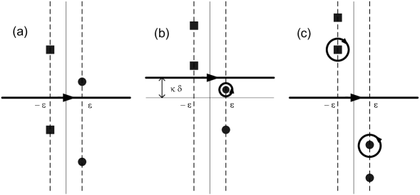
Figure 3: Integration paths in the complex $q_{4}$ plane for: a) $q_{3}>\sqrt{\frac{p_{0}^{2}}{4}-m^{2}}+\delta$; b) $\sqrt{\frac{p_{0}^{2}}{4}-m^{2}}-\delta<q_{3}<\sqrt{\frac{p_{0}^{2}}{4}-m^{2}}+\delta$ ; c) $q_{3}<\sqrt{\frac{p_{0}^{2}}{4}-m^{2}}-\delta$. The constant $\kappa$ is an arbitrary real number satisfying $\kappa>1$.

which is an integral of the type given in Eq. (A.1). Note that the poles of the propagators are such that this situation belongs to case (a), with $S_{i}=m$. For $p_{0}>2\,m$ the straightforward transformation from Minkowski to Euclidean space mentioned above cannot be done, since some poles go through the integration contours. The question is whether the result of the well-defined Miskowskian integral (A.9) can be still recovered if one starts with the Euclidean integral (A.10), which is ill-defined for $p_{0}>2\,m$ due to the presence of a pinch point at $(q_{3}^{p},q_{4}^{p})=(\sqrt{p_{0}^{2}/4-m^{2}},0)$. It is not hard to prove that the answer is yes, once the $q_{4}$ integration contours and the pole positions are conveniently modified. The procedure requires to introduce two small parameters, $\epsilon$ and $\delta$, and take the limit $\delta\to 0^{+}$, $\epsilon\to 0^{+}$ at the end of the calculation. The parameter $\epsilon$ is used to shift the poles of $D^{+}$ and $D^{-}$ (see Fig. 3), whereas $\delta$ is used to split the $q_{3}$ integration interval in three subintervals: the first region corresponds to $q_{3}>q_{3}^{p}+\delta$, the second to $q_{3}^{p}-\delta<q_{3}<q_{3}^{p}+\delta$ and the third to $q_{3}<q_{3}^{p}-\delta$. For each $q_{3}$ region we define a different $q_{4}$ integration contour, as represented in Fig. 3 (in the second region, Fig. 3b, also an arbitrary constant $\kappa>1$ is introduced). In fact, in the first and third regions the limit $\epsilon\rightarrow 0^{+}$ can be taken even before performing the integrations. These two $q_{3}$ regions give the full contribution to the real part of the result. However, more care has to be taken with the intermediate region, which is responsible for the full contribution to the imaginary part. For example —as it is well known from the “$i\,\epsilon$” Minkowskian formulation—, changing the sign of $\epsilon$ does not affect the real part of the result but does change the sign of the imaginary part.

The prescription just described can be now applied to regularize any loop integral of the form given in Eq. (A.1) in which $p_{0}>2S_{i}$. Let us consider first the case (a), for which the lowest set of poles has $S_{r}=0$ and the pinch point is located at $(q_{3}^{p},q_{4}^{p})=(\sqrt{p_{0}^{2}/4-S_{i}^{2}},0)$. Defining $C^{(a)}(-p_{0}^{2})$ as an integral of the form given by Eq. (A.1) for which only one set of purely imaginary poles contributes, we get

$${\rm Re}\left[C^{(a)}(-p_{0}^{2})\right] = \lim_{\delta\rightarrow 0^{+}}\left\{\;R^{(a)}(-p_{0}^{2},\delta)+\int_{0}^{q_{3}^{p}-\delta}dq_{3}\int_{-\infty}^{\infty}dq_{4}\frac{q_{3}^{2}\ F(q_{3},q_{4},p_{0})}{\left[(q^{+})^{2}+\Sigma^{2}(q^{+})\right]\left[(q^{-})^{2}+\Sigma^{2}(q^{-})\right]}\right.$$ (A.11)

$$\ \ +\left.\int_{q_{3}^{p}+\delta}^{\infty}\ dq_{3}\int_{-\infty}^{\infty}dq_{4}\frac{q_{3}^{2}\ F(q_{3},q_{4},p_{0})}{\left[(q^{+})^{2}+\Sigma^{2}(q^{+})\right]\left[(q^{-})^{2}+\Sigma^{2}(q^{-})\right]}\;\right\}$$

$${\rm Im}\left[C^{(a)}(-p_{0}^{2})\right] = -\frac{\pi^{2}}{2p_{0}}\;\ \frac{q_{3}^{p}\ F(q_{3}^{p},0,p_{0})}{\left[1+\left.\frac{\partial\Sigma^{2}(q)}{\partial q^{2}}\right|_{q^{2}=-S^{2}_{i}}\right]^{2}}\ \ .$$ (A.12)

Here $R^{(a)}(-p_{0}^{2},\delta)$ is the so-called “residue contribution”, responsible for the cancellation of the divergence appearing in the integrals in (A.11) in the limit $\delta\to 0^{+}$. Its explicit expression reads

$$R^{(a)}(-p_{0}^{2},\delta)\ =\ 2\pi\int_{0}^{q_{3}^{p}-\delta}\frac{dq_{3}}{\sqrt{q_{3}^{2}+S_{i}^{2}}}\ \ {\rm Re}\!\left[\frac{q_{3}^{2}\;F(q_{3},q_{4},p_{0})}{\left[1+\frac{\partial\Sigma^{2}(q^{-})}{\partial(q^{-})^{2}}\right]\left[(q^{+})^{2}+\Sigma^{2}(q^{+})\right]}\right]_{q_{4}=q_{4}^{(2)}=i(\frac{p_{0}}{2}-\sqrt{q_{3}^{2}+S_{i}^{2}})}\ .$$ (A.13)

For case (b) we have to extend the previous analysis to the situation in which the poles are complex even in the limit $\epsilon\to 0^{+}$. In this case there is an ambiguity on how to extend the “$i\,\epsilon$” prescription already in Minkowski space. Here we will follow the suggestion made in Ref. CLOP69 , in which opposite signs of $\epsilon$ are used for each pole and its hermitian conjugate (both defined in Minkowski space). In our Euclidean framework, this corresponds to choose different signs of $\epsilon$ for sets $p_{4}^{(i)}$ and ${p_{4}^{(i)}}^{\prime}$. It is not hard to see that with this prescription the contributions to the imaginary part of the quark loop integral coming from both sets of poles cancel each other. In this way, defining $C^{(b)}(-p_{0}^{2})$ as an integral of the type given in Eq. (A.1) for which only one set of complex poles contributes, we get

$${\rm Im}\left[C^{(b)}(-p_{0}^{2})\right]=0\ .$$ (A.14)

For the real part one obtains an expression similar to Eq. (A.11), just replacing $R^{(a)}(-p_{0}^{2},\delta)$ by $R^{(b)}(-p_{0}^{2},\delta)$, with

$$R^{(b)}(-p_{0}^{2},\delta)\ =\ 4\pi\int_{0}^{q_{3}^{p}-\delta}\!\!dq_{3}\ \ {\rm Re}\!\left[\frac{q_{3}^{2}\ F(q_{3},q_{4},p_{0})}{\left[1+\frac{\partial\Sigma^{2}(q^{-})}{\partial(q^{-})^{2}}\right]\left[(q^{+})^{2}+\Sigma^{2}(q^{+})\right](iq_{4}+\frac{p_{0}}{2})}\right]_{q_{4}=q_{4}^{(2)}}\ .$$ (A.15)

In principle, the extension of the present analysis to the situation in which further sets of poles are relevant is rather straightforward. However, some care has to be taken if one has more than one set of purely imaginary poles, since in that case double poles might show up for $p_{0}>S_{i}^{1}+S_{i}^{2}$.

One is faced with a similar problem in the calculation of the $\eta^{\prime}\to\gamma\gamma$ decay constant $g_{\eta^{\prime}\gamma\gamma}$, where the loop integral $I_{u}(m_{\eta^{\prime}}^{2})$ defined by Eq. (50) is divergent for $m_{\eta^{\prime}}>2\,S_{i}$. Though the situation is slightly more involved (one finds two pinch points instead of one), our regularization prescriptions can be trivially extended to include this case. In the same way, the method could be extended to more complicated situations, as e.g. those found in Schwinger-Dyson type of calculations RW94 ; BPT03 . Finally, we note that although our prescription has some similarities with that used in Ref. PB98 , the regularization procedure is not exactly the same. In the $(q_{3},q_{4})$ integral which appears in Eq. (A.11) the excluded region around the pinch point is a slide of infinite size in the $q_{4}$ direction and size $2\delta$ in the $q_{3}$ direction, as opposed to the circular region of radius $\delta$ used in Ref. PB98 . This leads to some minor differences in the numerical values of the regulated integrals.

		Gaussian					Lorentzian
Set		GI	GII	GIII	GIV		LI	LII	LIII	LIV	Empirical
$\bar{m}$	[ MeV ]	8.5	8.5	8.5	7.5		4.0	4.0	4.0	3.5	(3.4 - 7.4)
$m_{s}$	[ MeV ]	223	223	223	199		112	110	112	100	(108 - 209)
$\Lambda$	[ MeV ]	709	709	709	768		1013	1013	1013	1110
$G\,\Lambda^{2}$		10.99	11.44	10.80	10.43		14.68	16.76	14.96	14.05
$-H\,\Lambda^{5}$		295.3	275.4	303.7	305.1		743.4	573.8	720.4	821.0
-$<\bar{u}u>^{1/3}$	[ MeV ]	211	211	211	220		275	275	275	288
-$<\bar{s}s>^{1/3}$	[ MeV ]	186	187	185	204		297	307	299	314
$\Sigma_{u}(0)$	[ MeV ]	313	313	313	295		299	299	300	281
$\Sigma_{s}(0)$	[ MeV ]	650	662	645	607		562	615	569	518
$m_{\pi}$	[ MeV ]	$139^{*}$	$139^{*}$	$139^{*}$	$139^{*}$		$139^{*}$	$139^{*}$	$139^{*}$	$139^{*}$	139
$m_{K}$	[ MeV ]	$495^{*}$	$495^{*}$	$495^{*}$	$495^{*}$		$495^{*}$	$495^{*}$	$495^{*}$	$495^{*}$	495
$m_{\eta}$	[ MeV ]	517	505	521	522		543	513	540	545	547
$m_{\eta^{\prime}}$	[ MeV ]	$958^{*}$	879	1007	$958^{*}$		$958^{*}$	778	908	$958^{*}$	958
$G_{\pi q}$		3.28	3.28	3.28	3.09		3.13	3.13	3.13	2.94
$G_{Kq}$		3.47	3.52	3.45	3.21		3.05	3.24	3.08	2.80
$G_{\eta q}$		3.07	3.03	3.08	2.83		2.74	2.69	2.74	2.49
$G_{\eta^{\prime}q}$		1.62	2.01	1.21			1.36	2.21	1.13
$f_{\pi}$	[ MeV ]	$93.3^{*}$	$93.3^{*}$	$93.3^{*}$	$93.3^{*}$		$93.3^{*}$	$93.3^{*}$	$93.3^{*}$	$93.3^{*}$	93.3
$f_{K}/f_{\pi}$		1.29	1.29	1.29	1.29		1.25	1.28	1.26	1.25	1.22
$g_{\pi\gamma\gamma}^{2}$	[ GeV-2 ]	0.073	0.073	0.073	0.074		0.074	0.074	0.074	0.074	$0.075\pm 0.005$
$g_{\eta\gamma\gamma}^{2}$	[ GeV-2 ]	0.095	0.106	0.091	0.094		0.072	0.108	0.075	0.075	$0.067\pm 0.006$
$g_{\eta^{\prime}\gamma\gamma}^{2}$	[ GeV-2 ]	0.141	$0.116^{*}$	$0.116^{*}$			0.278	$0.116^{*}$	$0.116^{*}$		$0.116\pm 0.005$

Table 1: Numerical results for quark effective masses and condensates, and pseudoscalar meson masses and decay parameters. The light quark mass $\bar{m}$ has been taken as input, and the parameters $m_{s}$, $\Lambda$, $G$ and $H$ have been chosen so as to reproduce the empirical values of pion and kaon masses, the pion decay constant $f_{\pi}$ and, alternatively, the $\eta^{\prime}$ mass or the measured value of $g_{\eta^{\prime}\gamma\gamma}^{2}$ (marked with ^∗).

Set	GI	GII	GIII	GIV		LI	LII	LIII	LIV	$\begin{array}[]{c}{\rm Theory\ \ \&}\\ {\rm Phenomenology}\end{array}$
$f_{8}/f_{\pi}$	1.33	1.34	1.32			1.32	1.36	1.31		(1.2 - 1.4)
$f_{0}/f_{\pi}$	1.28	1.18	1.18			1.64	1.18	1.05		(1.0 - 1.3)
$\theta_{8}$	$-14.2^{\circ}$	$-19.7^{\circ}$	$-10.0^{\circ}$			$-11.7^{\circ}$	$-25.4^{\circ}$	$-10.6^{\circ}$		$-$($22^{\circ}$ - $19^{\circ}$)
$\theta_{0}$	$-2.14^{\circ}$	$-5.25^{\circ}$	$-1.17^{\circ}$			$1.66^{\circ}$	$-6.52^{\circ}$	1.60∘		$-$($10^{\circ}$ - $0^{\circ}$)
$\theta_{\eta}$	4.65	1.81	5.69	5.32		7.69	$-0.72$	6.90	8.00
$\theta_{\eta^{\prime}}$	$-50.0$	$-47.1$	$-52.4$			$-48.4$	$-44.6$	$-50.6$

Table 2: Numerical results for $\eta$ and $\eta^{\prime}$ weak decay parameters and state mixing angles, according to the definitions given by Eqs. (31) and (69).

Figure 1: Absolute values of the inverse meson propagators as functions of the momentum. The full line corresponds to $G_{\pi}$, the dashed line to $G_{K}$, the dotted line to $G_{\eta}$ and the dashed-dotted line to $G_{\eta^{\prime}}$. The upper panel corresponds to Set GI and the lower one to Set GIV. In both cases the insertions show a detail of the low momentum region where the zeros corresponding to the ground state pion, kaon and eta mesons occur.

Figure 2: Schematic distribution in the complex $q_{4}$-plane of the poles corresponding to the lowest $S_{i}$ set for: a) $\bar{\sigma}<\bar{\sigma}_{c}$ ; b) $\bar{\sigma}>\bar{\sigma}_{c}$. In both cases the dots indicate the poles of $D^{+}$ and the squares those of $D^{-}$. These distributions correspond to a value of $p_{0}<2S_{i}$. The arrows indicate the movement of the poles as $p_{0}$ increases.

References

- (1) Y. Nambu and G. Jona-Lasinio, Phys. Rev. 122, 345 (1961); Phys. Rev. 124, 246 (1961).
- (2) V. Bernard, R.L. Jaffe and U.G. Meissner, Phys. Lett. B 198, 92 (1987); Nucl. Phys. B 308, 753 (1988).
- (3) T. Kunihiro and T. Hatsuda, Phys. Lett. B 206, 385 (1988) [Erratum-ibid. 210, 278 (1988)]; T. Hatsuda and T. Kunihiro, Z. Phys. C 51, 49 (1991).
- (4) S. Klimt, M. Lutz, U. Vogl and W.Weise, Nucl. Phys. A 516, 429 (1990).
- (5) M. Takizawa, K. Tsushima, Y. Kohyama and K. Kubodera, Nucl. Phys. A 507, 611 (1990).
- (6) U. Vogl and W. Weise, Prog. Part. Nucl. Phys. 27, 195 (1991); S. Klevansky, Rev. Mod. Phys. 64, 649 (1992); T. Hatsuda and T. Kunihiro, Phys. Rep. 247, 221 (1994).
- (7) G. Ripka, Quarks bound by chiral fields (Oxford University Press, Oxford, 1997).
- (8) T. Schafer and E.V. Schuryak, Rev. Mod. Phys. 70, 323 (1998).
- (9) C.D. Roberts and A.G. Williams, Prog. Part. Nucl. Phys. 33, 477 (1994); C.D. Roberts and S.M. Schmidt, Prog. Part. Nucl. Phys. 45, S1 (2000).
- (10) E. Ruiz Arriola and L.L. Salcedo, Phys. Lett. B 450, 225 (1999).
- (11) G. Ripka, Nucl. Phys. A 683, 463 (2001); R.S. Plant and M.C. Birse, Nucl. Phys. A 703, 717 (2002).
- (12) R.D. Bowler and M.C. Birse, Nucl. Phys. A 582, 655 (1995)
- (13) R.S.Plant and M.C. Birse, Nucl. Phys. A 628, 607 (1998).
- (14) W. Broniowski, B. Golli and G. Ripka, Nucl. Phys. A703, 667 (2002).
- (15) A.H. Rezaeian, N.R. Walet and M.C. Birse, arXiv:hep-ph/0310013.
- (16) I. General, D. Gomez Dumm and N.N. Scoccola, Phys. Lett. B 506, 267 (2001); D. Gomez Dumm and N.N. Scoccola, Phys. Rev. D 65, 074021 (2002).
- (17) J.W. Bos, J.H. Koch and H.W.L. Naus, Phys. Rev. C 44, 485 (1991).
- (18) Particle Data Group, K. Hagiwara et al., Phys. Rev. D 66, 010001 (2002).
- (19) J. Gasser, Ann. of Phys. 136, 62 (1981); T. Hatsuda and T. Kunihiro, Nucl. Phys. B 387, 715 (1992).
- (20) It can be seen that our expressions for reduce to the result quoted in Appendix A of Ref. PB98 , where the steps leading to Eq. (65) are given in detail.
- (21) J. Gasser and H. Leutwyler, Phys. Rept. 87, 77 (1982); L. J. Reinders, H. Rubinstein and S. Yazaki, Phys. Rept. 127, 1 (1985).
- (22) L. Giusti, C. Hoelbling and C. Rebbi, Phys. Rev. D 64, 054501 (2001); P. Hasenfratz, S. Hauswirth, T. Jorg, F. Niedermayer and K. Holland, Nucl. Phys. B 643, 280 (2002); P. Hernandez, K. Jansen, L. Lellouch and H. Wittig, Nucl. Phys. Proc. Suppl. 106, 766 (2002); T-W. Chui and T-H. Hsieh, Nucl. Phys. B 673, 217 (2003)
- (23) T. Feldmann, Int. J. Mod. Phys. A 15, 159 (2000).
- (24) H. Leutwyler, Nucl. Phys. Proc. Suppl. 64, 223 (1998); R. Kaiser and H. Leutwyler, in Non-perturbative Methods in Quantum Field Theory, edited by A.W. Schreiber, A.G. Williams and A.W. Thomas (World Scientific, Singapore, 1998), arXiv:hep-ph/9806336.
- (25) T. Feldmann, P. Kroll and B. Stech, Phys. Rev. D 58, 114006 (1998); Phys. Lett. B 449, 339 (1999).
- (26) R. Escribano and J.-M. Frère, Phys. Lett. B 459, 288 (1999).
- (27) K. Naito, Y. Nemoto, M. Takizawa, K. Yoshida and M. Oka, Phys. Rev. C 61 065201 (2000).
- (28) Here and in what follows we use the term “complex pole” to indicate a pole for which both real and imaginary parts are different from zero.
- (29) R.E. Cutkosky, P.V. Landschoff, D.I. Olive and J.C. Polkinghorne, Nucl. Phys. B 12, 281 (1969).
- (30) M.S. Bhagwat, M.A. Pichowsky and P.C. Tandy, Phys. Rev. D 67, 054019 (2003).