Estimates of Light Quark Masses from Lattice QCD and QCD Sum rules

Abstract

This talk reviews the progress made in the determination of the light quark masses using lattice QCD and QCD sum rules. Based on preliminary calculations with three flavors of dynamical quarks, the lattice estimate is $m_{s}=75(15)$ MeV, a tantalizingly low value. On the other hand the leading estimates from scalar and pseudo-scalar sum rules are $99(16)$ and $100(12)$ MeV respectively. The $\tau$-decay sum rule estimates depend very sensitively on the value of $|V_{us}|$. The central values from different analyses lie in the range $115-120$ MeV if unitarity of CKM matrix is imposed, and in the range $100-105$ MeV if the Particle Data Group values for $|V_{us}|$ are used. I also give my reasons for why the lattice result is not yet in conflict with rigorous lower bounds from sum rule analyses.

1 Introduction

Quark masses are important fundamental parameters of the standard model. Our ability to extract them from first principle calculations of QCD will signal the onset of quantitative control over the non-perturbative aspects of QCD. In this talk I will summarize the current status of the extraction of light quark masses. All results for quark masses will be in the $\overline{\rm MS}$ scheme at scale 2 GeV. Most of the time will be devoted to a review of the lattice results. A brief summary of sum-rule calculations will also be presented. A more detailed version of this review is being prepared in collaboration with Tanmoy Bhattacharya and Kim Maltman [1].

Of the light quark masses, I will concentrate entirely on the strange quark mass. The reason is that, at present, estimates of the ratios from chiral perturbation theory

$$\frac{2m_{s}}{m_{u}+m_{d}} = 24.4(1.5)$$

$$\frac{m_{u}}{m_{d}} = 0.553(43)$$ (1)

are more accurate than the lattice results. Using them to extract $m_{u}$ and $m_{d}$, once $m_{s}$ is known, avoids some of the uncertainties due to chiral extrapolations in lattice calculations, and of ignoring electromagnetic effects in the simulations.

There is a recent result on the charm quark mass that deserves mention. I mention this to also highlight the fact that current lattice calculations indicate that the the whole interval $m_{u,d}-m_{c}$ can be handled by the techniques used for light quarks. Consequently, charm quark can be simulated on the lattice with small discretization errors. Following this approach, the ALPHA collaboration has presented, in the quenched approximation, the ratio [2]

$$\frac{m_{c}}{m_{s}}=12.0(5)\,.$$ (2)

The advantage of their calculation, based on the Schrödinger functional approach and using the fully $O(a)$ improved theory, is that they convert lattice masses to renormalization group invariant masses using a non-perturbative method, thus avoiding the problem of the perturbative determination of the scale dependent renormalization constant $Z_{m}^{0}$ at scales $1/a=2-4$ GeV and the subsequent matching of the lattice to a continuum regularization scheme at these scales. They find $m_{c}^{\overline{\rm MS}}(2{\rm GeV})=1.301(34)$ GeV, which compares well with the recent estimate $m_{c}^{\overline{\rm MS}}(2{\rm GeV})=1.26(4)(12)$ GeV by the SPQcdR collaboration [3].

2 Lattice QCD

A self-consistent determination of quark masses using lattice QCD will be equivalent to the validation of QCD as the correct theory of strong interactions. In ideal lattice QCD simulations we need to dial six input parameters in the generation of background gauge configurations and then calculate quark propagators on them. These are the gauge coupling $g$, and the masses for up, down, strange, charm, and bottom quarks. The top quark is neglected because it is too heavy and too short lived. If we had petaflop scale computers we could carry out simuations with three light and two heavy flavors of dynamical quarks with masses tuned to roughly their physical values $m_{u}$, $m_{d}$, $m_{s}$, $m_{c}$, and $m_{b}$. The inclusion of heavier quarks, charm and bottom, in the generation of background gauge configurations, however, are unlikely to significantly affect the vacuum structure and can therefore be safely neglected in the update for $Q^{2}$ much less than $9$ (or $100$) GeV². To study their interactions, charm and bottom quarks are incorporated at the stage of calculating quark propagators on these background gauge configurations. Thus simulations with three light dynamical flavors are the goal of lattice calculations.

Correlation functions in Euclidean space-time, from which various properties of hadrons are extracted, are constructed by tying together these quark propagators and gauge link variables in appropriate combinations. For example the hadronic spectrum and associated decay constants are extracted from two-point correlation functions with the appropriate quantum numbers. The masses of hadrons, at least of the stable ones and of those with very narrow widths, are determined from the rate of fall-off of these correlation functions at large Euclidean time. If QCD is the correct theory, these should agree with experiments up to electromagnetic corrections which are neglected in current simulations.

Unfortunately, today’s computers are not powerful enough to carry out calculations with physical values of up and down quark masses. Instead, quarks heavier than their physical values, $i.e.$ in the range $m_{s}/8-m_{s}$, have been studied. Also, isospin breaking and electromagnetic effects have been neglected, $i.e.$, simulations have been done with $m_{u}=m_{d}$ and electric charge turned off. From these simulations one extracts physical results by extrapolation in the up and down quark masses. The calculated hadron masses or decay constants are expressed as an expansion in quark masses using expressions derived from chiral perturbation theory. Once the coefficients of these chiral expansions, which are related to the low energy constants in the chiral Lagrangian, are determined then one has an overcomplete set of relations (because the number of hadronic observables are much larger than the input parameters) between experimentally measurable quantities and quark masses. Using these relations, extrapolations to the physical values of hadron masses or decay constants specify the physical quark masses. A self-consistent determination of the quark masses in terms of hadron masses or vice versa would validate QCD.

The success of this program requires that three conditions be met. First, the simulations should be done with three flavors of dynamical quarks and the input masses for all three quarks (both in the update and in the construction of external quark propagators, $i.e.$, sea and valence quarks) should be light enough to lie within the range of validity of the $O(p^{4})$ chiral Lagrangian [4, 5, 6]. This condition guarantees that the extracted chiral coefficients are the same as in QCD and reliable. Second, the simulations should be done at lattice scales small enough that discretization errors can be neglected or can be removed by a reliable extrapolation of the data to $a=0$. Third, simulations should be done on large enough lattices so that finite volume effects are negligible.

There are two ways in which the renormalized quark mass at scale $\mu$ is defined using lattice simulations done at scale $1/a$:

$$m_{R}(\mu) = Z_{m}(\mu,a)\ m(a)$$

$$(m_{1}+m_{2})_{R}(\mu) = \frac{Z_{A}}{Z_{P}(\mu,a)}\frac{\langle 0\mid\partial_{4}A_{4}(t)J(0)\mid 0\rangle}{\langle 0\mid P_{a}(t)J(0)\mid 0\rangle}\,.$$

The first method is based on the vector Ward identity and $m(a)$ is the bare lattice mass. The second method exploits the axial Ward identity and uses two-point correlation functions with source $J$ having pseudoscalar quantum numbers. For lattice formulations with an exact chiral symmetry, $e.g.$ staggered fermions, the two methods are identical. The connection between results obtained in the lattice regularization scheme and some continuum scheme like $\overline{\rm MS}$ used by phenomenologists is contained in the $Z^{\prime}s$. Their calculation introduces an additional source of systematic error in all quantities whose renormalization constants are different in the two schemes; spectral quantities (hadron masses) which do not get renormalized are an exception. I later discuss the quantitative effect on quark masses of the renormalization factors needed to connect lattice results to those in the $\overline{\rm MS}$ scheme.

In this talk I will analyze the state-of-the-art lattice data and discuss their reliability with respect to the following sources of systematic errors.

• The number and masses of dynamical quarks used in the update of gauge configurations.

• Chiral extrapolations to physical quark masses.

• Continuum extrapolations to $a=0$.

• The uncertainty in the calculation of the renormalization constant. In particular I will discuss the difference in estimates of masses between using 1-loop perturbative estimate, the one obtained in the RI/MOM scheme, and the fully non-perturbative one using the Schrödinger functional method.

3 State-of-the-art quenched results

The state-of-the-art quenched results are summarized in Table 1. Two recent results deserve some elaboration (I have not included results from domain wall [7] or overlap [8] fermions as they are still preliminary and do not include a continuum extrapolation).

(i) Results from the SPQcdR collaboration [9] supercede all previous estimates from the ROME group [10, 11], which is why the latter are not included in Table 1. The new calculations improve on previous results in the following ways. (i) The SPQcdR calculations have been done using the non-perturbative $O(a)$ improved Sheikholeslami-Wohlert action at four values of the coupling, $\beta=6.0$, $6.2$, $6.4$ and $6.45$. Over this range the lattice scale changes roughly by a factor of two ($0.1\to 0.051$ fermi), so a reliable extrapolation to the continuum limit has been carried out. (ii) The N³LO (4-loop) relation is used to connect the RI/MOM scheme to the $\overline{\rm MS}$ scheme for the renormalization constants, as well as in the running of the masses to the final scale $2$ GeV. (iii) Results using both the vector and axial Ward identity method have been computed and compared.

	Action	$\bar{m}$	$m_{s}(M_{K})$	$m_{s}(M_{\phi})$	scale $1/a$
	Renorm.	$=(m_{u}+m_{d})/2$
JLQCD	Staggered	$4.23(29)$	$106(7)$	$129(12)$	$M_{\rho}$
(1999)[12]	RI/MOM
CPPACS	Wilson	$4.57(18)$	$116(3)$	$144(6)$	$M_{\rho}$
(1999)[13]	1-loop TI
CP-PACS	Iwasaki+SW	$4.37^{+13}_{-16}$	$111^{+3}_{-4}$	$132^{+4}_{-5}$	$M_{\rho}$
(2000)[14]	1-loop TI
ALPHA-UKQCD	O(a) SW		$97(4)$		$f_{K}$
(1999) [15]	SF
QCDSF	O(a) SW	$4.4(2)$	$105(4)$		$r_{0}$
(1999)[16]	SF
QCDSF	Wilson	$3.8(6)$	$87(15)$		$r_{0}$
(1999)[16]	RI/MOM
SPQcdR	O(a) SW	$4.4(1)(4)$	$106(2)(8)$		$r_{0}$
(2002)[9]	RI/MOM

Table 1: State-of-the-art quenched results for quark masses. The labels for the action used are: $O(a)$ SW for non-perturbative $O(a)$ improved Sheikhholeslami-Wohlert (SW) fermion action, and Iwasaki for an improved gauge action. The renormalization factors are calculated using the 1-loop perturbation theory with Tadpole Improvement (TI) or the non-perturbative RI/MOM and Schrodinger functional (SF) schemes. The quantity used to set the lattice spacing $a$ is listed in the last column with $r_{0}=0.5$ fermi obtained from the static force relation $r\partial V(r)/\partial r|_{r=r_{0}}=1.65$ [17]. All estimates are based on extrapolation to the continuum limit. $m_{s}(M_{K})$ and $m_{s}(M_{\phi})$ refer to the strange quark mass extracted using $M_{K}$ or $M_{\phi}$ to fix it.

(ii) The QCDSF collaboration is in the process of updating their 1999 estimates of the strange quark mass [16]. They use the same methodology and the same values of coupling, $\beta=6.0$, $6.2$, and $6.4$, as the SPQcdR collaboration [9], so their results will provide a detailed consistency check. Their latest unpublished quenched estimate is $r_{0}m_{s}^{RGI}=0.341(2)$ which translates to $m_{s}^{\overline{\rm MS}}\approx 100$ MeV.

Discussion: The estimates in Table 1 show a wide range of values that seem to depend on the lattice action, the quantity used to set the scale and the quark masses, and the renormalization constant. What I would like to emphasize is that this spread does not imply that the lattice calculations are in conflict, simply that in the quenched approximation one does not expect consistent results and the spread is a manifestation of that.

Within the lattice community it has been known for some time that, in the quenched approximation, there is a roughly $10\%$ variation in estimates of the quark masses depending on the quantity used to set the lattice scale $a$ ($r_{0}$ or $M_{\rho}$ or $f_{K}$ or $M_{N}$ etc.). This was quantitatively demonstrated by Wittig at LATTICE 2002 [18] who converted the results from the four best simulations by SPQcdR, JLQCD, CP-PACS, and ALPHA-UKQCD collaborations to a common scale set by $r_{0}$. The result, shown in Table 2, is that these four estimates of $m_{s}$, when extracted using a common scale setting quantity, i.e., evaluating $m_{s}/r_{0}$ in the continuum limit, show a much smaller variation and agree within errors. This indicates that the dependence on the fermion action, fitting procedures, statistics, and renormalization constants (perturbative versus non-perturbative) used in the calculations are much smaller effects.

The other lessons we have learned from quenched simulations are:

• Quenched simulations do not give consistent estimates of quark masses. Estimates depend on the hadronic states used to set the quark masses. For example $m_{s}$ set using $M_{K}$ differs by $15-20\%$ from that set using $M_{K^{*}}$ or $M_{\phi}$ when the scale is set by $M_{\rho}$. Thus, quark masses are sensitive probes of the effects of dynamical quarks.

• With non-perturbative results for $Z^{\prime}s$ in hand we can evaluate how well 1-loop tadpole improved perturbation theory works to convert lattice results to $\overline{\rm MS}$ scheme. We find that 1-loop estimates work to within $5\%$ for VWI method, $i.e.$ $Z_{m}$ for Wilson like fermions, and at about $10\%$ for the AWI method . Given that the rest of the errors, once a common scale setting quantity is used, are of this order, the collapse of results in Table 2 to a roughly common value is not surprising.

The bottom line is that quenched simulations have allowed us to refine the numerical methods, and to understand and quantify all other sources of errors to within $5\%$. So removing this approximation becomes the next step in obtaining precise estimates.

Ref.	$m_{s}(Q^{\prime})$	$Q^{\prime}$	$F$	$m_{s}(r_{0})$
JLQCD	$106(7)$	$M_{\rho}$	$0.90(1)$	$95(6)$
CP-PACS	$114(2)(^{+6}_{-3})$	$M_{\rho}$	$0.86(2)$	$98(2)(^{+6}_{-3})$
SPQcdR	$106(2)(8)$	$M_{K^{*}}$	$0.87(3)$	$92(2)(7)$
ALPHA-UKQCD	$\phantom{1}97(4)$	$f_{K}$	$1.02(2)$	$99(4)$

Table 2: Comparison by Wittig of $m_{s}(\overline{\rm MS},{\rm 2\ GeV},M_{K})$ from quenched simulations by the JLQCD, CP-PACS, SPQcdR, and ALPHA-UKQCD collaborations. Given are the original estimates and the scale setting quantity $Q^{\prime}$, conversion factor $F$ from $Q^{\prime}$ to $r_{0}$, and the converted mass.

	Action	$\bar{m}$	$m_{s}(M_{K})$	$m_{s}(M_{\phi})$	scale $1/a$
	Renorm				(GeV)
JLQCD	Wilson+SW	$3.22(4)$	$84.5(1.1)$	$96.4(2.2)$	$M_{\rho}$
(2002)[19]	1-loop TI				(2.22)
CP-PACS	Iwasaki+SW	$3.45^{+0.14}_{-0.20}$	$89^{+3}_{-6}$	$90^{+5}_{-11}$	$M_{\rho}$
(2000)[20]	1-loop TI				($a\to 0$)
QCDSF-UKQCD	O(a) SW	$3.5(2)$	$90^{+5}_{-10}$		$r_{0}$
(2003)[21]	1-loop TI				$[1.9-2.2]$
QCDSF-UKQCD	O(a) SW		$85(1)$		$r_{0}$
(2003)[22]	RI-MOM				$[1.9-2.2]$

Table 3: Recent $N_{f}=2$ results for quark masses.

4 Discussion of $N_{f}=2$ results

The CP-PACS collaboration [20, 23] set the stage for large scale simulations with dynamical fermions by providing results that are of comparable quality to quenched simulations with respect to statistics, number of quark masses used in the simulations, and in the number of values of lattice spacings used in the continuum extrapolations. Their estimates displayed a number of desired features. The most striking was that estimates of the strange quark mass from four different methods $--$ using the axial and vector Ward identity definition of the quark mass and using either $M_{K}$ or $M_{\phi}$ to fix $m_{s}$ $--$ were in agreement. The numbers ranged from $86.9(2.3)$ to $90.3(4.9)$.

The JLQCD collaboration [19] has provided another measurement of quark masses with two dynamical flavors that complements results by the CP-PACS collaboration [20]. There are, however, a number of technical differences in the two sets of calculations. The CP-PACS calculation used the 1-loop mean field improved value of $c_{SW}$ in the fermion action, whereas the JLQCD uses the non-perturbative value. CP-PACS used the Iwasaki improved gauge action whereas JLQCD uses the unimproved Wilson (plaquette) action. CP-PACS had results at three values of the lattice scale ($a\approx 0.22$, $0.16$, and $0.11$ fermi) while JLQCD provide data at a single point at $a=0.0887(11)$ fermi. (The fourth point in the CP-PACS calculation at $a=0.0865$ fermi was used only as a consistency check because it has small statistics.)

The JLQCD estimates spoil some of the nice consistency shown by the CPPACS analysis. In particular if one combines data from the two calculations, the extrapolations of AWI($M_{K}$) and AWI($M_{\phi}$) estimates give $\approx 88$ MeV, whereas those from VWI($M_{K}$) and VWI($M_{\phi}$) extrapolate to $\approx 93$ MeV as shown in Fig. 1. JLQCD quotes their AWI($M_{K}$) value, $84.5{}^{+12.0}_{-1.7}$, as their best estimate assuming this method has the smallest $a$ dependence. The difference between the AWI($M_{K}$) and VWI($M_{K}$) values is taken as an estimate of the systematic uncertainty. I discuss these data further below.

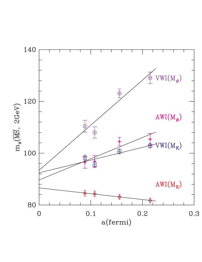
Figure 1: Estimates of $m_{s}$ from the $N_{f}=2$ simulations by the CP-PACS and JLQCD (points on the finest lattice with $a\approx 0.09$ fermi) collaborations. Linear extrapolation to the continuum limit are shown for all four definitions of the quark mass.

The QCDSF collaboration [24] is in the process of updating their $N_{f}=2$ estimate given in [21]. The piece of the calculation still missing is a non-perturbative evaluation of the renormalization constants. They should be finishing this calculation soon, meanwhile their unpublished estimate, using perturbative estimates of renormalization constants, is $m_{s}^{\overline{\rm MS}}(2\ {\rm GeV})=85(11)$ MeV.

5 Continuum extrapolation

I will use the data and fits in Figure 1 to illustrate the systematic uncertainty associated with the continuum extrapolation and the associated issues of renormalization constants and the partially quenched approximation. Even though, as mentioned above, the point at $a\approx 0.09$ fermi is obtained with a different gauge and fermion action and therefore expected to have a different coefficient for the $O(a)$ errors, nevertheless, I have taken the liberty of making a common fit to qualitatively illustrate how [in]sensitive the conclusions are to current errors in individual points and to a linear fit that extends all the way to $a=0.22$ fermi.

The extrapolated values are based on a linear fit to four points. Keeping a linear term is appropriate since $O(a)$ errors have not been fully removed from the action or the currents, however this does not mean that higher order corrections are unimportant. Looking at the fits it clear that more high precision data at smaller values of $a$ are required to include/exclude higher order terms with a reasonable degree of confidence. Given the spread, JLQCD choose $84.5{}^{+12.0}_{-1.7}$ as their best estimate of $m_{s}$ since $AWI(M_{K})$ values show very little $a$ dependence. The different extrapolations are accommodated by associating a large positive systematic uncertainty to the central value.

It is interesting to note that the two estimates using $AWI$ extrapolate to $\approx 88$ MeV, whereas those using the $VWI$ to $\approx 93$ MeV. This suggests that the difference is not due to using $M_{K}$ versus $M_{\phi}$ but due to $AWI$ versus $VWI$ methods. There are two differences between these methods that could account for this discrepancy. First, the renormalization constants are different for lattice actions that do not preserve chiral symmetry (one needs $Z_{A}/Z_{P}$ in the $AWI$ and $Z_{m}=1/Z_{s}$ for the $VWI$); and second, there is an extra complication, in the case of the $VWI$ method, coming from having to determine $\kappa_{c}$, the critical value of the hopping parameter corresponding to zero quark mass. The problem of the determination of $\kappa_{c}$ using VWI from partially quenched simulations leads to an additive shift in estimates of quark masses. A comparative analysis of $m_{u,d}$ suggests that this issue leads to no more than $1$ MeV uncertainty in estimate of quark masses, so I concentrate on the $Z^{\prime}s$ for the explanation.

Repeating the CP-PACS and JLQCD analysis shows that most of the difference comes from the renormalization factor that connects lattice results to those in the $\overline{\rm MS}$ scheme at 2 GeV, i.e. $Z_{VWI}\approx 1.1Z_{AWI}$. Another way of stating this is that the lattice values of $m_{s}$ are roughly the same for the two methods; it is the connection between the two schemes which leads to majority of the difference. What we know from non-perturbative calculations of renormalization constants in the quenched approximation is that $Z_{P}$ is significantly (by about $10\%$) overestimated by tadpole-improved 1-loop perturbation theory, whereas $Z_{S}$ and $Z_{A}$ are much better approximated. If we assume that the same is true in the $N_{f}=2$ case, then correcting for this in the CP-PACS/JLQCD data would boost the $AWI$ results by about $10\%$ since $m_{R}=(Z_{A}/Z_{P})m$, and explain the difference between $AWI$ and $VWI$ results. In that case all four fits would extrapolate to $m_{s}(\overline{\rm MS},{\rm 2\ GeV})\approx 93$ MeV. In the absence of non-perturbative estimates for the renormalization constants, my conclusion, based on the CP-PACS and JLQCD results, is to take a flat distribution between $84-93$ MeV as the best estimate for $m_{s}$. This range also incorporates the QCDSF-UKQCD estimates.

Note that my reservation of $\sim 10\%$ uncertainty due to the 1-loop $Z$’s does not apply to the four sets of quenched data analyzed by Wittig because none of those calculations use, simultaneously, the AWI method and 1-loop estimates for $Z$’s.

6 $N_{f}=3$ results

Simulations with three flavors of dynamical quarks, all with masses $\leq m_{s}$, represent a qualitatively big step forward. The reason for this favorable situation is that the coefficients of the chiral Lagrangian determined by fitting data for observables obtained at different masses to the corresponding chiral expansions are the same as QCD [4, 5, 6]. Thus, as long as the simulations are done within the region of validity of $O(p^{4})$ $\chi$PT, we can extract physical results even from simulations done at $3-18$ times $m_{d}$.

Very recently preliminary results from simulations with three flavors were reported by the MILC [25] and CP-PACS/JLQCD [26] collaborations at LATTICE 2003. These are summarized in Table 4.

	Action	$\bar{m}$	$m_{s}(M_{K})$	scale $1/a$
	Renorm		AWI	(GeV)
JLQCD	Iwasaki+SW	$2.89(6)$	$75.6(3.4)$	$M_{\rho}$
(2003)[26]	1-loop TI			($2.05(5)$)
MILC	AsqTad	$2.5(1)$	$66(1)$	$M_{\rho}$
(2003)[27]	1-loop TI			($1.6$)
MILC	AsqTad	$2.6(1)$	$68(1)$	$M_{\rho}$
(2003)[27]	1-loop TI			($2.2$)

Table 4: Recent $N_{f}=3$ results for quark masses. AsqTad is a perturbatively improved version of Staggered fermions which reduces “taste” symmetry breaking. The quoted errors in the MILC results include both statistical and those due to varying $q^{*}$ in the 1-loop matching between $(1/a\to 2/a)$. The entries in the last column give the quantity used to set the scale and its value in GeV.

The CP-PACS/JLQCD collaboration [26] employ the same analysis as in their $N_{f}=2$ study [20] and use an improved gauge action as well as an $O(a)$ improved Wilson quark action. Analysis of the AWI data give $m_{s}=75.6(3.4)$, and the analysis of the VWI data is not complete as the determination of $\kappa_{c}$ is not yet under control. Their most accurate number is from the AWI($M_{K}$) method and AWI($M_{\phi}$) gives a consistent value but with much larger errors. The difference between the two estimates is folded into the error estimate.

Two major issues remain with the CP-PACS/JLQCD results. These are (i) residual discretization errors as the calculation has been done at only one lattice scale and (ii) the use of 1-loop tadpole improved $Z$’s. To address the first requires more data which is a matter of time. On the second issue my reservation, that the 1-loop perturbation theory overestimates $Z_{P}$ by $\sim 10\%$, resurfaces. If this reservation holds up then their estimate could be as high as $85$ MeV. Based on these reservations, their numbers suggest the rather large range $m_{s}=70-90$ MeV.

The MILC Collaboration results [25] are obtained using improved staggered fermions. (An older estimate, based on an independent analysis of a sub-set of this MILC data, was reported by Hein [28] at LATTICE 2002.) I have listed the results under AWI even though for staggered like fermions (lattice fermions with a chiral symmetry) the AWI and VWI methods are identical. A major step forward in the MILC analysis is they perform a combined fit to data for $M_{K}^{2}$ at two sets of lattices (coarse and fine) using a staggered $\chi$PT expression that includes discretization and taste symmetry violating corrections

$$\frac{(M_{K^{+}_{5}}^{1-loop})^{2}}{\mu\,(m_{x}+m_{y})}$$

$$= 1+\frac{1}{16\pi^{2}f^{2}}\Big{(}[-\frac{2a^{2}\delta_{V}^{\prime}}{M^{2}_{\eta_{V}^{\prime}}-M^{2}_{\eta_{V}}}(l(M^{2}_{\eta_{V}})-l(M^{2}_{\eta_{V}^{\prime}}))]$$

$$\hphantom{+++++1}+[V\to A]+\frac{2}{3}l(M^{2}_{\eta_{I}})\Big{)}$$

$$\hphantom{1}+\frac{16\mu}{f^{2}}(2L_{8}-L_{5})(m_{x}+m_{y})$$

$$\hphantom{1}+\frac{32\mu}{f^{2}}(2L_{6}-L_{4})(2m_{q}+m_{s})\ +\ a^{2}C\,,$$

where $m_{x}+m_{y}$ is the sum of the masses of the two valence quarks. Even though fit to a complicated S$\chi$PT expression with 44-46 parameter, having very precise data allows them to extract the central values and the associated errors estimates reliably. Their best estimates are $m_{u,d}=2.7(6)$ and $m_{s}=70(15)$ MeV. A very large part of the error comes from the fact that to the 1-loop estimate for $Z_{m}$ they assign an overall $\sim 20\%$ uncertainty due to the neglected $O(\alpha^{2})$ terms. In my opinion this is a conservative estimate of the $O(\alpha_{s}^{2})$ uncertainty, especially since the 1-loop coefficient for the improved (AsqTad) staggered fermions is small, (${\mathrel{\raise 2.0pt\hbox to8.0pt{\raise-5.0pt\hbox{$\sim$}\hss{$<$}}}}0.12\alpha_{s}$) [28]. The authors are clearly keeping in mind the lesson learned from quenched unimproved staggered fermions where that 1-loop perturbation theory underestimated $Z_{m}$ (and thus $m_{s}$) by almost $30\%$.

A concern with the MILC simulation is the lack of a “proof” that the staggered fermion action describes four degenerate flavors in the continuum limit. Furthermore, there is the potential problem of loss of locality of the action when taking the square root and the fourth root of the staggered determinant to simulate two plus one dynamical flavors. These issues are being investigated [29] now that all other sources of errors are understood, and the community is moving towards providing precision results. Unfortunately, as of now there is no airtight argument that settles these issues.

Based on these two preliminary calculations, and if forced to quote a single number, my choice is $m_{s}=75(15)$ MeV. This estimate is certainly very exciting and provocative. Furthermore, with simulations at more values of the lattice spacing and with different fermion formulations coming on line, this exciting result will soon be refined.

As mentioned before, the power of $N_{f}=3$ analysis, provided all quark masses are small such that 1-loop $\chi$PT applies, is that the chiral parameters are those of physical QCD. Thus, in addition to estimates for quark masses the MILC collaboration [25] extract the Gasser-Leutwyler constants from their fit. In particular they find that

$$2L_{8}-L_{5}=-0.1(1)({}^{+1}_{-3})\times 10^{-3}\,.$$ (3)

This is significantly outside the range

$$-3.4\times 10^{-3}\ {\mathrel{\raise 2.0pt\hbox to8.0pt{\raise-5.0pt\hbox{$\sim$}\hss{$<$}}}}\ 2L_{8}-L_{5}\ {\mathrel{\raise 2.0pt\hbox to8.0pt{\raise-5.0pt\hbox{$\sim$}\hss{$<$}}}}\ -1.8\times 10^{-3}$$ (4)

acceptable for $m_{u}=0$. The same conclusion has been reached by the OSU group [30]. In short, lattice results do not favor the possibility that $m_{u}=0$ is the solution of the strong CP problem.

7 $m_{s}$ from QCD Sum Rules

Three types of sum-rules have commonly been employed to determine light quark masses. They are (i) Borel (Laplace) transformed sum rules (BSR’s); (ii) finite energy sum rules (FESR’s); and (iii) Hadronic $\tau$ decay sum rules (these $\tau$-decay SR are a special case of FESR) .

The starting point for the pseudoscalar and scalar QCD sum rules are the axial and vector Ward identities

$$\partial^{\mu}A^{us}_{\mu} = (m_{s}+m_{u})\ i:\bar{s}\gamma_{5}u:$$

$$\partial^{\mu}V^{us}_{\mu} = (m_{s}-m_{u})\ i:\bar{s}u:$$

and the corresponding integrated 2-point correlation functions, $e.g.$

$$\Psi_{5}(q^{2})$$

$$\equiv \hphantom{(m_{d})^{2}}i\int\,d^{4}xe^{iq\cdot x}\langle 0|T\{\partial^{\mu}A_{\mu}^{{\dagger}}(x),\partial^{\nu}A_{\nu}(0)\}|0\rangle,$$

$$= (m_{d}+m_{u})^{2}i\int\,d^{4}xe^{iq\cdot x}\langle 0|T\{P^{{\dagger}}(x),P(0)\}|0\rangle\,.$$

$\Psi(q^{2})$ and $\Psi_{5}(q^{2})$ are analytic on the complex $q^{2}$ plane with poles and cuts along the positive real axis. They can be calculated using OPE and perturbation theory for large $|q^{2}|$ (say $q^{2}>s_{0}$) and away from the cut. They are related, through dispersion relations, to spectral functions, for example, $\rho_{5}(s)={\rm Im}\Psi_{5}(s)/\pi$.

Finite energy sum rules are based on the observation that the spectral function has singularities (poles and cuts) only along the real axis as shown in Fig. 2. The contour integral shown in Fig. 2 is zero so

$$\int_{0}^{s_{0}}w(s)\rho_{hadronic}\ ds=\frac{-1}{2\pi i}\oint_{|s|=s_{0}}w(s)\Pi_{PQCD}\ ds$$

The left hand side (discontinuity along the real axis) is evaluated using a combination of experimental input and modeling for the spectral function. The right hand side is evaluated using the OPE and perturbation theory for the dominant mass-dimension $D=0$ term. The scheme and scale ($s_{0}$) used for the perturbation defines the scheme and scale in which the quark mass is defined. $w(s)$ are conveniently chosen weights designed to improve convergence. Since the OPE is expected to break down near the real axis at $s_{0}$, recent analyses have employed “pinched” weights like $w(s)=(1-s/s_{0})^{n}$ that have a zero at $s=s_{0}$. The resulting sum rules are called pinched FESR.

Figure 2: The contour integral used in finite energy sum rules. The poles and cuts are along the real axis. Duality refers to the matching, on average, between the perturbative and hadronic ansätze.

In the Borel transformed sum rule one integrates the spectral function of the vector current along the real axis

$${\cal B}[\Pi]_{OPE} = \hphantom{+}\int_{0}^{s_{0}}e^{-s/M^{2}}\rho_{hadronic}ds$$

$$+\int_{s_{0}}^{\infty}e^{-s/M^{2}}\rho_{OPE}ds\,.$$

For the strange scalar channel the $l.h.s.$ is proportional to $(m_{s}-m_{u})^{2}$. In the OPE, the dominant $D=0$ term is evaluated using perturbation theory and defines the scheme and scale at which the mass is evaluated. The breakup of the integral on the $r.h.s$ depends on a suitable choice of $s_{0}$. It has to be large enough that the integral of the perturbative estimate of the OPE (second term) is reliable and yet small enough that there is experimental data on the spectral function up to that point. Otherwise there is a large gap in which $\rho$ can, at best, be modeled. Second, the answer should be independent of the Borel Mass $M$. One cannot choose M too small as the transform gives more weight to the low $s/M^{2}$ region. This is good on the $r.h.s.$ but unfortunately on the $l.h.s.$ it enhances the uncertainty of the higher dimensional operators. At the same time we want $s_{0}/M^{2}>1$ so that the unknown contribution of the “continuum” to $\rho_{hadronic}$ is suppressed.

There are three important questions central to the reliability of all sum rules analyses.

• How well does the operator product expansion converge? Furthermore, are the non-perturbative corrections, like quark and gluon condensates, instanton effects, and neglected higher order terms in the OPE small?

• How well is the perturbative expansion for the leading terms in the OPE known and how well does it converge at the scale $s_{0}$?

• How well is the hadronic spectral function determined through a combination of experimental data and modeling?

With respect to these points two major improvements have occurred over the last five years. These include

• The perturbative series for the scalar and the pseudo-scalar sum-rules are now known up to $\alpha_{s}^{3}$ (four loops) [31].

• Better models of the hadronic spectral function have been developed that satisfy a number of consistency checks.

A number of hurdles, mainly in our ability to determine the phenomenological spectral function, remain.

• In the pseudoscalar sum rule for $m_{u}+m_{d}$, the hadronic spectral function includes the masses and widths of the kaon, $K(1460)$, and $K(1830)$ resonances (to extract $m_{u}+m_{d}$ from the pion channel the corresponding states are $\pi,\pi(1300),\pi(1770)$). What are not known are the decay constants of the $K(1460)$, and $K(1830)$ and their relative phase. Also, the $K\pi\pi$ continuum is modeled using resonant forms with or without chiral perturbation theory modifications. The prospects of new data to improve the spectral function are small.

• In the scalar sum rule for $m_{s}$, the spectral function starts at the $K\pi$ threshold. Also known are the masses and widths of the $K_{0}^{\ast}(1430)$ and $K_{0}^{\ast}(1950)$ resonances. Below the $K_{0}^{\ast}(1430)$ threshold, the spectral function is fairly well determined using the $K_{e3}$ data and the $K\pi$ scattering phases. What is not known is whether there is significant phase variation near and above the $K_{0}^{\ast}(1950)$ resonance. Prospects of improving $\rho(s)$ from B-factories are marginal.

Without going into details which will be presented in [1], my conclusion, based on the Borel and finite energy sum rules, is that the most complete analysis for $m_{s}$ from the scalar channel gives $m_{s}=99(16)$ MeV [32]. For the pseudo-scalar channel it is $m_{s}=100(12)$ [33].

The $\tau$-decay sum rules utilizes data for the ratio of semi-hadronic to leptonic decay rate

$$R_{\tau}^{V/A,ij}=\frac{\Gamma[\tau^{-}\to\nu_{\tau}{\rm hadrons}_{V/A,ij}(\gamma)]}{\Gamma[\tau^{-}\to\nu_{\tau}e^{-}\bar{\nu}_{e}(\gamma)]}$$

where $V/A,ij$ denotes the flavor ($ud$ or $us$) of the Vector $(V)$ or Axial $(A)$ current. Experimental data gives access to the $u,d$ and $u,s$ spectral functions. The perturbative series for the $1+0$ part of the $D=2$ $\tau$-decay sum rule are known only up to $\alpha_{s}^{2}$ (three loops). The $0$ part of the $\tau$-decay series is known to $\alpha_{s}^{3}$. Here $0$ and $1$ refer to the angular momentum of the hadronic part. A summary of current estimates of $m_{s}$ from hadronic $\tau$-decay sum rules is given in Table 5 [34].

	$m_{s}(2\ {\rm GeV})$ (MeV)
Reference	Original	CKMU input	CKMN input
CKP98 [35]	$145\pm 36$ ($|V_{us}|=.2213$)	$116\pm 31$	$99\pm 34$
KKP00 [36]	$125\pm 28$ ($|V_{us}|=.2218$)	$120\pm 28$	$106\pm 32$
KM00 [37]	$115\pm 17$ ($|V_{us}|=.2196$)	$110\pm 16$	$100\pm 18$
CDGHPP01 [38]	$116^{+20}_{-25}\ \$ ($|V_{us}|=.2215$)
GPJSP03 [39]		$117\pm 17$	$103\pm 17$

Table 5: Evolution of results for $m_{s}(2\ {\rm GeV})$ obtained using hadronic $\tau$ decay data. The “original” values are those obtained by the authors along with $|V_{us}|$ used. The updates of these values use the CKMU ($|V_{us}|=0.2225\pm 0.0021$) and CKMN ($|V_{us}|=0.2196\pm 0.0026$). All CKM[U,N] input sets correspond to $R^{V+A}_{\tau;us}=.163$ and branching fractions $B_{e}=.1783$, $B_{\mu}=.1737$. From this one gets $R^{V+A}_{\tau;ud}=3.471$. All use $\alpha_{s}(m_{\tau}^{2})=.334$ and, with the exception of KKP00 [36], the CDGHPP01 [38] truncation prescription. Experimental and theoretical errors have been combined in quadrature.

The interesting feature to note, notwithstanding the many improvements, are that the results in Table 5 have been fairly constant over the last three years. The central value of $m_{s}$ has stayed in the range $115-120$ MeV if unitarity of CKM matrix is imposed, and $m_{s}=100-105$ MeV if the Particle Data Group values for $|V_{us}|$ are used. Both estimates have errors of about $20$ MeV. In short, the results are very sensitive to the value of $|V_{us}|$, and the difference between the two estimates is of the same size as all the other uncertainties combined.

Drawbacks of the $\tau$-decay sum rule are: (i) The Cabibbo suppressed hadronic $\tau$-decay data has not been separately resolved into $J=0$ and $J=1$ contributions and (ii) there is large uncertainty in the perturbative behavior of the scalar component. Some progress in reducing a sub-set of these uncertainties was recently reported by the GPJSP collaboration [39] where they used a phenomenological parameterization for the scalar and pseudoscalar spectral function in the OPE. These new results, shown in Table 5, are, nevertheless, consistent with previous estimates.

In terms of future prospects, we expect significant improvement in the measured $\tau$-decay spectral function, especially above the $K^{\ast}$. Meanwhile, it is clear that, at least as far as the central value of $m_{s}$ is concerned, pushing it significantly below $100$ MeV is disfavored by the sum-rules analyses.

8 Lower bounds on quark masses

Even though the sum rule and Lattice QCD estimates overlap within combined uncertainties, the current best estimate of the lattice result ($75\pm 15$) MeV is tantalizingly small. The following question is often raised. Does this lattice number violate rigorous lower bounds predicted from a sum-rule analysis? My answer is NO and I give a brief justification for this [1].

The most stringent bound predicted is the “quadratic” bound obtained by Lellouch, de Rafael and Taron [40]. It predicts, assuming perturbation theory becomes reliable by $Q=2$ GeV, that $m_{s}({\overline{\rm MS}},2\ {\rm GeV})>100$ MeV. The Achilles’ heel of this analysis is that the perturbative expression that enters into the quadratic bound has very large coefficients [33]:

$$3{\cal F}_{0}{\cal F}_{2}-2({\cal F}_{1})^{2} = 1+\frac{25}{3}a(Q^{2})+61.79a^{2}(Q^{2})$$ (5)

$$\hphantom{0}+\ 517.15a^{3}(Q^{2})+\ldots$$

$$= 1+0.83+0.61+0.51+\ldots\,.$$

where the second expression has been evaluated at $Q=2$ GeV with $a\equiv\alpha_{s}/\pi\approx 0.1$. Pushing $Q\geq 2.5$ GeV already lowers the bound to $m_{s}({\overline{\rm MS}},2\ {\rm GeV})>80$ MeV and going to a still safer value of $Q=3$ GeV where $\alpha_{s}/\pi=0.086$ gives $m_{s}({\overline{\rm MS}},2\ {\rm GeV})>60$ MeV. With such a poorly behaved series it becomes an article of faith as to what $Q$ is considered safe, and therefore what value to take as the lower bound.

There are two other bounds for which the perturbation theory is reasonable even for $Q\geq 1.4$ GeV. These are the $\Sigma_{0}\geq 0$ given in [40], and the “ratio” bound given in [41]. Assuming that perturbation theory is reliable at $Q=1.4$, both these bounds provide a much lower value, $i.e.$, $m_{s}({\overline{\rm MS}},2\ {\rm GeV})>80$ MeV.

My bottom line on these bounds is that we should be concerned only if lattice results go significantly below $m_{s}=70MeV$. So, the interesting question is which estimate will change over time? Will the sum rule estimate come down to match the lattice value of $\approx 75$ MeV, or will the lattice result rise to match the sum-rule value $m_{s}{\mathrel{\raise 2.0pt\hbox to8.0pt{\raise-5.0pt\hbox{$\sim$}\hss{$>$}}}}100$ MeV? Or will both change within their errors and come together in the middle? And finally, it will be interesting to understand which, if any, systematic error is being underestimated in the two methods.

References

- [1] T. Bhattacharya, R. Gupta and K. Maltman. In preparation.
- [2] ALPHA Collaboration, J. Rolf and S. Sint, JHEP 12 (2002) 007, hep-ph/0209255.
- [3] D. Becirevic, V. Lubicz and G. Martinelli, Phys. Lett. B524 (2002) 115, hep-ph/0107124.
- [4] S.R. Sharpe and N. Shoresh, Phys. Rev. D62 (2000) 094503, hep-lat/0006017.
- [5] S.R. Sharpe and N. Shoresh, Phys. Rev. D64 (2001) 114510, hep-lat/0108003.
- [6] S.R. Sharpe and R.S. Van de Water (2003), hep-lat/0308010.
- [7] RBC Collaboration, C. Dawson, Nucl. Phys. Proc. Suppl. 119 (2003) 314, hep-lat/0210005.
- [8] P. Hernandez, K. Jansen, L. Lellouch and H. Wittig, Nucl. Phys. Proc. Suppl. 106 (2002) 766, hep-lat/0110199.
- [9] D. Becirevic, V. Lubicz and C. Tarantino, Phys. Lett. B558 (2003) 69, hep-lat/0208003.
- [10] D. Becirevic et al., Phys. Lett. B444 (1998) 401, hep-lat/9807046.
- [11] D. Becirevic, G. Gimenez, V. Lubicz and G. Martinelli, Phys. Rev. D61 (2000) 114507, hep-lat/9909082.
- [12] JLQCD Collaboration, S. Aoki et al., Phys. Rev. Lett. 82 (1999) 4392, hep-lat/9901019.
- [13] CP-PACS Collaboration, S. Aoki et al., Phys. Rev. Lett. 84 (2000) 238, hep-lat/9904012.
- [14] CP-PACS Collaboration, A. Ali Khan et al., Phys. Rev. Lett. 90 (2003) 029902.
- [15] ALPHA Collaboration, J. Garden, J. Heitger, R. Sommer and H. Wittig, Nucl. Phys. B571 (2000) 237, hep-lat/9906013.
- [16] QCDSF Collaboration, M. Gockeler et al., Nucl. Phys. (Proc. Suppl.) 83-84 (2000) 173, hep-lat/9908005.
- [17] R. Sommer, Nucl. Phys. B411 (1994) 839, hep-lat/9310022.
- [18] H. Wittig, Nucl. Phys. Proc. Suppl. 94 (2002), hep-lat/0210025.
- [19] JLQCD Collaboration, S. Aoki et al. (2002), hep-lat/0212039.
- [20] CP-PACS Collaboration, A. Ali Khan et al., Phys. Rev. D65 (2002) 054505, hep-lat/0105015.
- [21] QCDSF Collaboration, D. Pleiter, Nucl. Phys. Proc. Suppl. 94 (2001) 265, hep-lat/0010063.
- [22] QCDSF Collaboration, G. Schierholz (2003). Presented at Lattice 2003.
- [23] CP-PACS Collaboration, A. Ali Khan et al., Phys. Rev. D67 (2003) 059901(E).
- [24] QCDSF Collaboration, M. Gockeler et al. (2003). Presented at Lattice 2003.
- [25] MILC Collaboration, C. Aubin et al. (2003), hep-lat/0309088.
- [26] CP-PACS and JLQCD Collaboration, T. Kaneko et al. (2003), hep-lat/0309137.
- [27] C. Aubin. Poster at Lattice 2003. See http://www.physics.wustl.edu/~cb/fpi_poster2003.pdf.
- [28] HPQCD Collaboration, J. Hein et al., Nucl. Phys. Proc. Suppl. 119 (2003) 317, hep-lat/0209077.
- [29] K. Jansen, H. Wittig and F. Knechtli, Work in progress.
- [30] D.R. Nelson, G.T. Fleming and G.W. Kilcup, Phys. Rev. Lett. 90 (2003) 021601, hep-lat/0112029.
- [31] K.G. Chetyrkin, Phys. Lett. B390 (1997) 309, hep-ph/9608318.
- [32] M. Jamin, J.A. Oller and A. Pich, Eur. Phys. J. C24 (2002) 237, hep-ph/0110194.
- [33] K. Maltman and J. Kambor, Phys. Rev. D65 (2002) 074013, hep-ph/0108227.
- [34] R. Gupta and K. Maltman, Int. J. Mod. Phys. A16S1B (2001) 591, hep-ph/0101132.
- [35] K.G. Chetyrkin, J.H. Kuhn and A.A. Pivovarov, Nucl. Phys. B533 (1998) 473, hep-ph/9805335.
- [36] J.G. Korner, F. Krajewski and A.A. Pivovarov, Eur. Phys. J. C20 (2001) 259, hep-ph/0003165.
- [37] J. Kambor and K. Maltman, Phys. Rev. D62 (2000) 093023, hep-ph/0005156.
- [38] S. Chen et al., Eur. Phys. J. C22 (2001) 31, hep-ph/0105253.
- [39] E. Gamiz et al., JHEP 01 (2003) 060, hep-ph/0212230.
- [40] L. Lellouch, E. de Rafael and J. Taron, Phys. Lett. B414 (1997) 195, hep-ph/9707523.
- [41] T. Bhattacharya, R. Gupta and K. Maltman, Phys. Rev. D57 (1998) 5455, hep-ph/9703455.