Loops and Power Counting in the High Density Effective Field Theory

Abstract

We discuss the high density effective theory of QCD. We concentrate on the problem of developing a consistent power counting scheme.

1 Introduction

The study of hadronic matter in the regime of high baryon density has led to the theoretical prediction of several new phases of strongly interacting matter, such as color superconducting quark matter and color-flavor locked matter [1, 2, 3, 4, 5, 6, 7, 8, 9]. These phases may be realized in nature in the cores of neutron stars. In order to study this possibility quantitatively we would like to develop a systematic framework that will allow us to determine the exact nature of the phase diagram as a function of the density, temperature, the quark masses, and the lepton chemical potentials, and to compute the low energy properties of these phases.

If the density is large then the Fermi momentum is much bigger than the QCD scale, $p_{F}=\mu\gg\Lambda_{QCD}$, and asymptotic freedom implies that the effective coupling is weak. It would then seem that such a framework is provided by weak perturbative QCD. It is well known, however, that a naive expansion in powers of $\alpha_{s}$ is not sufficient. Long range gauge boson exchanges lead to infrared divergencies that require resummation. In a degenerate Fermi system the effect of the BCS or other pairing instabilities have to be taken into account. And finally, in systems with broken global symmetries, the low energy properties of the system are governed by collective modes that carry the quantum numbers of the broken generators.

In order to address these problems it is natural to exploit the separation of scales provided by $\mu\gg g\mu\gg\Lambda_{QCD}$ in the normal phase, or $\mu\gg g\mu\gg\Delta\gg\Lambda_{QCD}$ in the superfluid phase. An effective field theory approach to phenomena near the Fermi surface was suggested by Hong [10, 11]. This approach was applied to a number of problems [12, 13, 14, 15], see [16] for a review. Even though a number of interesting results have been obtained there are a number of important conceptual issues that are not very well understood. These issues concern power counting, renormalization and matching. In this contribution we would like to study some of these issues in more detail.

2 High Density Effective Theory (HDET)

At high baryon density the relevant degrees of freedom are particle and hole excitations which move with the Fermi velocity $v$. Since the momentum $p\sim v\mu$ is large, typical soft scatterings cannot change the momentum by very much. An effective field theory of particles and holes in QCD is given by [10, 11, 13]

$${\cal L}=\sum_{v}\psi_{v}^{\dagger}(iv\cdot D)\psi_{v}-\frac{1}{4}G^{a}_{\mu\nu}G^{a}_{\mu\nu}+\ldots,$$ (1)

where $v_{\mu}=(1,\vec{v})$. The field describes particles and holes with momenta $p=\mu\vec{v}+l$, where $l\ll\mu$. We will write $l=l_{0}+l_{\|}+l_{\perp}$ with $\vec{l}_{\|}=\vec{v}(\vec{l}\cdot\vec{v})$ and $\vec{l}_{\perp}=\vec{l}-\vec{l}_{\|}$. In order to take into account the entire Fermi surface we have to cover the Fermi surface with patches labeled by the local Fermi velocity, see Fig. 1. The number of such patches is $n_{v}\sim(\mu^{2}/\Lambda_{\perp}^{2})$ where $\Lambda_{\perp}\ll\mu$ is the cutoff on the transverse momenta $l_{\perp}$.

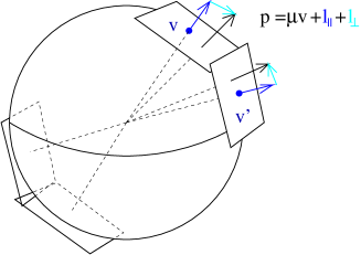
Figure 1: High density effective field theory description of excitations near the Fermi surface. The effective theory is defined on patches labeled by the local Fermi velocity $v$. Momenta are decomposed with respect to $v$, $\vec{p}=\mu\vec{v}+l_{\perp}+l_{||}$.

Higher order terms are suppressed by powers of $1/\mu$. As usual we have to consider all possible terms allowed by the symmetries of the underlying theory. At $O(1/\mu)$ we have

$${\cal L}=\sum_{v}\left\{-\frac{1}{2\mu}\psi_{v}^{\dagger}D_{\perp}^{2}\psi_{v}-ag\psi_{v}^{\dagger}\frac{\sigma^{\mu\nu}G_{\mu\nu}^{\perp}}{4\mu}\psi_{v}\right\}.$$ (2)

The coefficient of the first term is fixed by the dispersion relation of a fermion near the Fermi surface, $l_{0}=l_{\|}+l_{\perp}^{2}/(2\mu)+\ldots$. The coefficient of the second term is most easily determined by integrating out anti-particles at tree level. We find $a=1+O(g^{2})$, where the $O(g^{2})$ terms arise from higher order perturbative corrections. At higher order in $1/\mu$ there is an infinite tower of operators of the form $\mu^{-n}\psi^{\dagger}_{v}D_{\perp}^{2n_{1}}(\bar{v}\cdot D)^{n_{2}}\psi_{v}$ with $\bar{v}=(1,-\vec{v})$ and $n=2n_{1}+n_{2}-1$.

At $O(1/\mu^{2})$ the effective theory contains four-fermion operators

$${\cal L} = \frac{1}{\mu^{2}}\sum_{v_{i}}\sum_{\Gamma,\Gamma^{\prime}}c^{\Gamma\Gamma^{\prime}}(\vec{v}_{1}\cdot\vec{v}_{2},\vec{v}_{1}\cdot\vec{v}_{3},\vec{v}_{2}\cdot\vec{v}_{3})$$ (3)

$$\mbox{}\hskip 14.22636pt\cdot\Big{(}\psi_{v_{1}}\Gamma\psi_{v_{2}}\Big{)}\Big{(}\psi^{\dagger}_{v_{3}}\Gamma^{\prime}\psi^{\dagger}_{v_{4}}\Big{)}\delta(v_{1}+v_{2}-v_{3}-v_{4}).$$

The restriction $v_{1}+v_{2}=v_{3}+v_{4}$ allows two types of four-fermion operators, see Fig. 2. The first possibility is that both the incoming and outgoing fermion momenta are back-to-back. This corresponds to the BCS interaction

$${\cal L}=\frac{1}{\mu^{2}}\sum_{v,v^{\prime}}\sum_{\Gamma,\Gamma^{\prime}}V_{l}^{\Gamma\Gamma^{\prime}}R_{l}^{\Gamma\Gamma^{\prime}}(\vec{v}\cdot\vec{v}^{\prime})\Big{(}\psi_{v}\Gamma\psi_{-v}\Big{)}\Big{(}\psi^{\dagger}_{v^{\prime}}\Gamma^{\prime}\psi^{\dagger}_{-v^{\prime}}\Big{)},$$ (4)

where $\vec{v}\cdot\vec{v}^{\prime}=\cos\theta$ is the scattering angle and $R_{l}^{\Gamma\Gamma^{\prime}}(\vec{v}\cdot\vec{v}^{\prime})$ is a set of orthogonal polynomials that we will specify below. The second possibility is that the final momenta are equal to the initial momenta up to a rotation around the axis defined by the sum of the incoming momenta. The relevant four-fermion operator is

$${\cal L}=\frac{1}{\mu^{2}}\sum_{v,v^{\prime},\phi}\sum_{\Gamma,\Gamma^{\prime}}F_{l}^{\Gamma\Gamma^{\prime}}(\phi)R_{l}^{\Gamma\Gamma^{\prime}}(\vec{v}\cdot\vec{v}^{\prime})\Big{(}\psi_{v}\Gamma\psi_{v^{\prime}}\Big{)}\Big{(}\psi^{\dagger}_{\tilde{v}}\Gamma^{\prime}\psi^{\dagger}_{\tilde{v}^{\prime}}\Big{)},$$ (5)

where $\tilde{v},\tilde{v}^{\prime}$ are the vectors obtained from $v,v^{\prime}$ by a rotation around $v_{tot}=v+v^{\prime}$ by the angle $\phi$. In a system with short range interactions only the quantities $F_{l}(0)$ are known as Fermi liquid parameters. In QCD forward scattering is correctly reproduced by the leading order HDET lagrangian, but exchange terms have to be absorbed into four fermion operators [17].

The matrices $\Gamma,\Gamma^{\prime}$ describe the spin, color and flavor structure of the interaction. The spin structure is most easily discussed in terms of helicity amplitudes. As an example, we consider the BCS operators $(v,-v)\to(v^{\prime},-v^{\prime})$. The spins of the two quarks can be coupled to total spin zero or one. In the spin zero sector there are two possible helicity channels, $(++)\to(++)$ and $(++)\to(--)$ together with their parity partners $(+\leftrightarrow-)$. In the limit $m\to 0$ perturbative interactions only contribute to the helicity non-flip amplitude

$${\cal L} = \frac{1}{\mu^{2}}\sum_{v,v^{\prime}}V_{l}^{++}P_{l}(\vec{v}\cdot\vec{v}^{\prime})\Big{(}\psi_{v}\sigma_{2}H_{+}\psi_{-v}\Big{)}\Big{(}\psi^{\dagger}_{v^{\prime}}\sigma_{2}H_{+}\psi^{\dagger}_{-v^{\prime}}\Big{)}$$ (6)

$$\mbox{}\hskip 85.35826pt+(+\leftrightarrow-),$$

where $P_{l}(\cos\theta)$ are Legendre polynomials and $H_{\pm}$ are helicity projectors. Quark mass terms as well as non-perturbative effects associated with instantons induce helicity flip operators [14, 18]. These operators are suppressed by additional powers of $1/\mu$, but they have important physical effects. For example, helicity flip amplitudes determine the masses of Goldstone bosons in the CFL and 2SC phases.

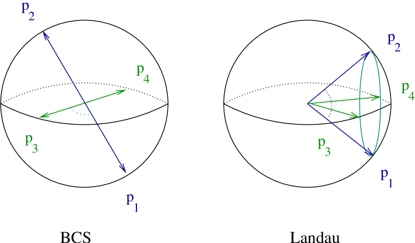
Figure 2: Kinematics of four-fermion operators in the effective theory.

In the spin one sector there is only one helicity channel $(+-)\to(+-)$. The corresponding BCS interaction is

$${\cal L} = \frac{1}{\mu^{2}}\sum_{v,v^{\prime}}V_{l}^{+-}d^{(l)}_{11}(\vec{v}\cdot\vec{v}^{\prime})\Big{(}\psi_{v}\sigma_{2}H_{-}\vec{\sigma}H_{+}\psi_{-v}\Big{)}$$ (7)

$$\mbox{}\hskip 28.45274pt\cdot\Big{(}\psi^{\dagger}_{v^{\prime}}\sigma_{2}H_{-}\vec{\sigma}H_{+}\psi^{\dagger}_{-v^{\prime}}\Big{)}+(+\leftrightarrow-),$$

where $d^{(l)}_{11}(\cos\theta)$ is the reduced Wigner D-function. In addition to the operators considered here there is, of course, an infinite tower of operators with more fermion fields or extra covariant derivatives.

3 Matching

The four-fermion operators in the effective theory can be determined by matching the quark-quark scattering amplitudes in the BCS and forward scattering kinematics. As an illustration we consider the leading order $O(g^{2})$ BCS amplitude in the spin zero color anti-triplet channel. The matching condition is

$$\int d\theta f^{++}_{HDET}(\theta)P_{l}(\theta)=\int d\theta f^{++}_{QCD}(\theta)P_{l}(\theta),$$ (8)

where $f^{++}(\theta)$ is the on-shell $(v,-v)\to(v^{\prime},-v^{\prime})$ scattering amplitude in the helicity $(++)\to(++)$ channel as a function of the scattering angle $cos\theta=v\cdot v^{\prime}$, see Fig. 3. The scattering amplitude in the effective theory contains almost collinear gluon exchanges which do not change the velocity label of the quarks as well as four-fermion operators which correspond to scattering involving different patches on the Fermi surface. The collinear contribution to the moments of the scattering amplitude depends on the cutoff $\Lambda_{\perp}$ which we impose on the transverse momenta inside a given velocity patch. Since the moments in the microscopic theory are independent of $\Lambda_{\perp}$ this dependence has to cancel against the cutoff dependence of the coefficients of the four-fermion operators.

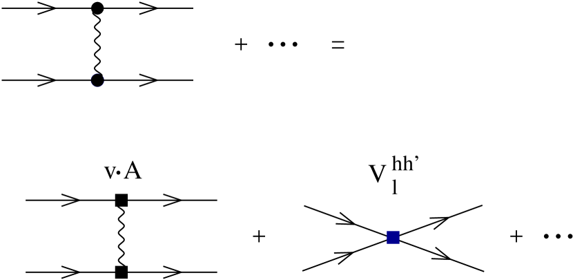
Figure 3: Matching condition for the four-fermion operators in the high density effective theory.

The matching condition is simplest for $\Lambda_{\perp}^{2}=2\mu^{2}$. The s-wave term is given by $V^{++}_{0}(\Lambda_{\perp}^{2}=2\mu^{2})=0$ up to corrections of $O(g^{4})$ [19]. The cutoff dependence of $V_{0}^{++}$ is controlled by the renormalization group equation

$$\Lambda_{\perp}^{2}\frac{d}{d\Lambda_{\perp}^{2}}V_{0}^{++}(\Lambda_{\perp}^{2})=\frac{g^{2}}{3}.$$ (9)

We can also compute the coefficients of four-fermion operators corresponding to higher partial wave and operators with non-zero spin. For example, the angular momentum $l=1$ terms in the helicity zero and one channels are given by

$$V^{++}_{1}(\Lambda_{\perp}^{2}=2\mu^{2}) = -6\frac{g^{2}}{3},$$ (10)

$$V^{+-}_{1}(\Lambda_{\perp}^{2}=2\mu^{2}) = -\frac{9}{2}\frac{2g^{2}}{3}.$$ (11)

We will see below that these results determine the relative magnitude of the BCS gap in channels with different spin and angular momentum [20, 21, 22].

4 Symmetries and Power Counting

In this section we shall discuss the symmetries of the high density effective theory and try to develop a systematic power counting. The high density effective theory has a number of similarities with the heavy quark (HQET) and soft collinear (SCET) effective field theories. As in both of these theories, the fermion field is characterized by a velocity label, and the kinetic term is of the form $v\cdot D$. Like SCET, HDET is a theory of ultra-relativistic particles and $v^{2}=0$. On the other hand, HDET has a number of symmetries that are more akin to non-relativistic field theories. For example, the leading order HDET effective lagrangian, equ. (1), has a SU(2) spin symmetry

$$\psi_{v}\to\exp(i\vec{\theta}\cdot\vec{\sigma})\psi_{v}.$$ (12)

Superficially, terms that break this symmetry are suppressed by powers of $1/\mu$. We shall see that this is not true, however. Hard dense loops modify the power counting in HDET, and SU(2) violating terms are not suppressed by powers of $\mu$, but only by powers of the coupling constant, $g$. The approximate spin symmetry of the HDET lagrangian has nevertheless important physical consequences. For example, to leading logarithmic accuracy the BCS gap in the spin zero and spin one channel are the same.

The HDET lagrangian also possesses a reparametrization invariance

$$\vec{v} \to \vec{v}+\vec{\epsilon}/\mu,$$ (13)

$$\vec{l} \to \vec{l}-\vec{\epsilon},$$ (14)

$$\psi_{v} \to \psi_{v}+\delta\psi_{v},$$ (15)

which reflects our freedom in choosing the local Fermi velocity. Note that in order to keep $v^{2}=0$ we have to choose $\vec{v}\cdot\vec{\epsilon}=0$. As usual, reparametrization invariance fixes the coefficients of certain higher order terms in the effective lagrangian.

We now come to the issue of power counting. The power counting in HDET has a number of similarities with the power counting in NRQCD and SCET, see [23, 24] for a discussion of these effective theories. We first discuss a “naive” attempt to count powers of the small scale $l$. In the naive power counting we assume that $v\cdot D$ scales as $l$, $\psi_{v}$ scales as $l^{3/2}$, $A_{\mu}$ scales as $l$, and every loop integral scales as $l^{4}$. We also assume that $\vec{D}_{\perp},\bar{v}\cdot D\sim l$. In this case it is easy to see that a general diagram with $V_{k}$ vertices of scaling dimension $k$ scales as $l^{\delta}$ with

$$\delta=4+\sum_{k}V_{k}(k-4).$$ (16)

A general vertex is of the form

$$\psi^{a}(v\cdot D)^{b}(\bar{v}\cdot D)^{c}(D_{\perp})^{d}(1/\mu)^{e},$$ (17)

and has mass dimension $3a/2+b+c+d-e=4$. Since $k=3a/2+b+c+d$ and $e\geq 0$ we have $k-4\geq 0$. This implies that the power counting is trivial: All diagrams constructed from the leading order lagrangian have the same scaling, all diagrams with higher order vertices are suppressed, and the degree of suppression is simply determined by the number and the scaling dimension of the vertices.

Figure 4: Counting hard loops in the effective field theory. If all (soft) gluon lines are removed the remaining fermionic loops contain sums over the velocity index.

Complication arise because not all loop diagrams scale as $l^{4}$. In fermion loops sums over patches and integrals over transverse momenta can combine to give integrals that are proportional to the surface area of the Fermi sphere,

$$\frac{1}{2\pi}\sum_{\vec{v}}\int\frac{d^{2}l_{\perp}}{(2\pi)^{2}}=\frac{\mu^{2}}{2\pi^{2}}\int\frac{d\Omega}{4\pi}.$$ (18)

These loop integrals scale as $l^{2}$, not $l^{4}$. In the following we will refer to loops that scale as $l^{2}$ as “hard loops” and loops that scale as $l^{4}$ as “soft loops”. In order to take this distinction into account we define $V_{k}^{S}$ and $V_{k}^{H}$ to be the number of soft and hard vertices of scaling dimension $k$. A vertex is called soft if it contains no fermion lines. In order to determine the $l$ counting of a general diagram in the effective theory we remove all gluon lines from the graph, see Fig. 4. We denote the number of connected pieces of the remaining graph by $N_{C}$. Using Euler identities for both the initial and the reduced graph we find that the diagram scales as $l^{\delta}$ with

$$\delta=\sum_{i}\left[(k-4)V_{k}^{S}+(k-2-f_{k})V_{k}^{H}\right]+E_{Q}+4-2N_{C}.$$ (19)

Here, $f_{k}$ denotes the number of fermion fields in a hard vertex, and $E_{Q}$ is the number of external quark lines. We observe that in general the scaling dimension $\delta$ still increases with the number of higher order vertices, but now there are two important exceptions.

First we observe that the number of disconnected fermion loops, $N_{C}$, reduces the power $\delta$. Each disconnected loop contains at least one power of the coupling constant, $g$, for every soft vertex. As a result, fermion loop insertions in gluon $n$-point functions spoil the power counting if the gluon momenta satisfy $l\sim g\mu$. This implies that for $l<g\mu$ the high density effective theory becomes non-perturbative and fermion loops in gluon $n$-point functions have to be resummed. We will see in the next section that this resummation leads to the familiar hard dense loop (HDL) effective action [25, 26].

Figure 5: Hard loop contribution to the gluon polarization function.

The second observation is that the power counting for hard vertices is modified by a factor that counts the number of fermion lines in the vertex. Using equ. (17) it is easy to see that four-fermion operators without extra derivatives are leading order ($k-2-f_{k}=0$), but terms with more than four fermion fields, or extra derivatives, are suppressed. This result is familiar from the effective field theory analysis of theories with short range interactions [27, 28].

5 Hard Loops

As an example of a hard dense loop diagram we consider the gluon two point function. At leading order in $g$ and $1/\mu$ we have

$$\Pi^{ab}_{\mu\nu}(p) = 2g^{2}N_{f}\frac{\delta^{ab}}{2}\sum_{\vec{v}}v_{\mu}v_{\nu}$$ (20)

$$\mbox{}\hskip 8.5359pt\cdot\int\frac{d^{4}k}{(2\pi)^{4}}\frac{1}{(k_{0}-l_{k})(k_{0}+p_{0}-l_{k+p})},$$

where $l_{k}=\vec{v}\cdot\vec{k}$. We note that taking the momentum of the external gluon to be small automatically selects almost forward scattering. We also observe that the gluon can interact with fermions of any Fermi velocity so that the polarization function involves a sum over all patches. After performing the $k_{0}$ integration we get

$$\Pi^{ab}_{\mu\nu}(p)=g^{2}N_{f}\delta^{ab}\sum_{\vec{v}}v_{\mu}v_{\nu}\int\frac{d^{2}l_{\perp}}{(2\pi)^{2}}\int\frac{dl_{k}}{2\pi}\frac{l_{p}}{p_{0}-l_{p}}\frac{\partial n_{k}}{\partial l_{k}},$$ (21)

where $n_{k}$ is the Fermi distribution function. We note that the $l_{k}$ integration is automatically dominated by small momenta. The integral over the transverse momenta combines with the sum over $\vec{v}$ as shown in equ. (18). We find

$$\Pi^{ab}_{\mu\nu}(p)=2m^{2}\delta^{ab}\int\frac{d\Omega}{4\pi}v_{\mu}v_{\nu}\left\{1-\frac{p_{0}}{p_{0}-l_{p}}\right\},$$ (22)

with $m^{2}=N_{f}g^{2}\mu^{2}/(4\pi^{2})$. This result has the correct dependence on $p_{0},l_{p}$, but it is not transverse. In the effective theory, this can be corrected by adding a counterterm [10]

$${\cal L}=\frac{1}{2}m^{2}\int\frac{d\Omega}{4\pi}(\vec{A}_{\perp})^{2}.$$ (23)

The appearance of this term is related to the fact that the $\mu^{-1}\psi^{\dagger}_{v}D_{\perp}^{2}\psi_{v}$ vertex gives a tadpole contribution which is not only enhanced because of the sum over $\vec{v}$, but also by a linear divergence in $l_{\|}$. Using similar arguments one can see that no additional counterterms are needed for $n\geq 3$ point functions. Putting everything together we find

$$\Pi_{\mu\nu}(p)=2m^{2}\int\frac{d\Omega}{4\pi}\left\{\delta_{\mu 0}\delta_{\nu 0}-\frac{v_{\mu}v_{\nu}p_{0}}{p_{0}-l_{p}}\right\}$$ (24)

which agrees with the standard HDL result. The gluonic three-point function can be computed in the same fashion. We get

$$\Gamma^{abc}_{\mu\nu\alpha}(p,q,r) = igf^{abc}2m^{2}\int\frac{d\Omega}{4\pi}v_{\mu}v_{\alpha}v_{\beta}$$ (25)

$$\hskip 8.5359pt\mbox{}\cdot\left\{\frac{q_{0}}{(q\cdot v)(p\cdot v)}-\frac{r_{0}}{(r\cdot v)(p\cdot v)}\right\}.$$

Higher order $n$-point functions can be computed in the same way, or by exploiting Ward identities. There is a simple generating functional for hard dense loops in gluon $n$-point functions which is given by [25, 26]

$${\cal L}_{HDL}=-m^{2}\int\frac{d\Omega}{4\pi}{\rm Tr}\,G_{\mu\alpha}\frac{\hat{P}^{\alpha}\hat{P}^{\beta}}{(\hat{P}\cdot D)^{2}}G^{\mu}_{\,\beta},$$ (26)

where the angular integral corresponds to an average over the direction of $\hat{P}_{\alpha}=(1,\hat{p})$. For momenta $l<g\mu$ we have to add ${\cal L}_{HDL}$ to ${\cal L}_{HDET}$. In order not to overcount diagrams we have to remove at the same time all diagrams that become disconnected if all soft gluon lines are deleted.

6 Soft Loops

As an example of a soft loop contribution in the high density effective theory we study the fermion self energy. At leading order, we have

$$\Sigma(p)=g^{2}C_{F}\int\frac{d^{4}k}{(2\pi)^{4}}\frac{1}{p_{0}+k_{0}-l_{p+k}}v_{\mu}v_{\nu}D_{\mu\nu}(k),$$ (27)

where $D_{\mu\nu}(k)$ is the gluon propagator. Soft contributions to the quark self energy are dominated by nearly forward scattering. Note that this loop integral does not involve a sum over patches. The contributions to the fermion self energy that arises from hard loop momenta is represented by the four-fermion operators given in equ. (5).

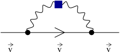
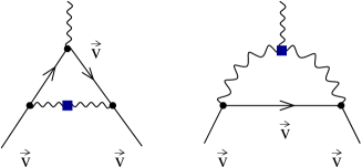
Figure 6: Leading order high density effective theory diagrams for the quark self energy and quark-gluon vertex function. The solid squares indicate HDL self energy and vertex corrections.

In the previous section we showed that for momenta $l<g\mu$ hard dense loop contributions to gluon $n$-point functions have to be resummed. The corresponding gluon propagator is given by

$$D_{\mu\nu}(k)=\frac{P_{\mu\nu}^{T}}{k^{2}-\Pi_{M}}+\frac{P_{\mu\nu}^{L}}{k^{2}-\Pi_{E}}$$ (28)

where $\Pi_{M}$ and $\Pi_{E}$ are the transverse and longitudinal self energies in the HDL limit. In the regime $|k_{0}|<|\vec{k}|<g\mu$ the self energies can be approximated by $\Pi_{E}=2m^{2}$ and $\Pi_{M}=i\frac{\pi}{2}m^{2}k_{0}/|\vec{k}|$. We note that in this regime the transverse self energy is much smaller than the longitudinal one, $\Pi_{M}<\Pi_{E}$. As a consequence the dominant part of the fermion self energy arises from transverse gluons. We have

$$\Sigma(p) = g^{2}C_{F}\int\frac{dl_{0}}{2\pi}\int\frac{l^{2}dl}{(2\pi)^{2}}$$ (29)

$$\mbox{}\cdot\int_{-1}^{1}dx\frac{1-x^{2}}{p_{0}+l_{0}-l_{p}-lx}\frac{1}{l_{0}^{2}-l^{2}+i\frac{\pi}{2}m^{2}\frac{l_{0}}{l}},$$

where $l_{p}=\vec{v}\cdot\vec{p}-\mu$ and $l_{k}=\vec{v}\cdot\vec{k}\equiv lx$ and $C_{F}=(N_{c}^{2}-1)/(2N_{c})$. To leading logarithmic accuracy we can ignore the difference between transverse and longitudinal cutoffs and set $\Lambda_{\perp}=\Lambda_{\|}=\Lambda$. We compute the integral by analytic continuation to euclidean space. In the limit $p_{4}\to 0$ the integral is independent of $l_{p}$ and given by [20, 29, 30, 31, 32, 33]

$$\Sigma(p_{4})\simeq\frac{g^{2}C_{F}p_{4}}{4\pi^{2}}\int\frac{l\,dl}{l^{2}+\frac{\pi}{2}m^{2}\frac{p_{4}}{l}}\simeq\frac{g^{2}C_{F}}{12\pi^{2}}p_{4}\log\left(\frac{\Lambda}{p_{4}}\right).$$ (30)

The calculation of the numerical constant inside the logarithm requires the determination of the coefficient of the four-fermion operator in equ. (5). We observe that the result $\Sigma\sim g^{2}l$ agrees with the naive power counting. However, we also note that the quark self energy has a logarithmic divergence which spoils the perturbative expansion for $l<\exp(-\bar{c}/g^{2})$.

A similar logarithmic divergence appears in the quark gluon vertex function. In order to compute this logarithm it is essential to take into account the HDL resummed gluon propagator and gluon three-point function, see Fig. 6. The logarithmic enhancement only appears in a specific kinematic configuration. We find [30]

$$\lim_{(p_{1})_{4}\to(p_{2})_{4}}\lim_{l_{p_{1}}\to l_{p_{2}}}\Gamma_{\alpha}(p_{1},p_{2})=\frac{g^{3}C_{F}v_{\alpha}}{12\pi^{2}}\log\left(\frac{\Lambda}{p_{4}}\right),$$ (31)

where $p_{1},p_{2}$ are the momenta of the fermions. In all other kinematic limits the vertex correction is of order $g^{3}$, not $g^{3}\log(l)$.

7 Color Superconductivity

Soft dense loop corrections to the fermion self energy and the quark-gluon vertex function become comparable to the free propagator and the free vertex at the scale $E\sim\mu\exp(-\bar{c}/g^{2})$. This implies that at this scale soft dense loops have to be resummed. Physically, this resummation corresponds to the study of non-Fermi liquid effects in dense quark matter [33, 34, 35, 36]. However, before non-Fermi liquid effects become important the quark-quark interaction in the BCS channel becomes singular. The scale of superfluidity is $E\sim\mu\exp(-c/g)$ [37].

The resummation of the quark-quark scattering amplitude in the BCS channel leads to the formation of a non-zero gap in the single particle spectrum. We can take this effect into account in the high density effective theory by including a tree level gap term

$${\cal L}=\Delta\,R_{l}^{\Gamma}(\vec{v}\cdot\hat{\Delta})\psi_{-v}\sigma_{2}\Gamma\psi_{v}+h.c..$$ (32)

Here, $\Gamma$ is any of the helicity structures introduced in Sect. 2, $R_{l}^{\Gamma}(x)$ is the corresponding angular factor and $\hat{\Delta}$ is a unit vector. The magnitude of the gap is determined variationally, by requiring the free energy to be stationary order by order in perturbation theory.

At leading order in the high density effective theory the variational principle for the gap $\Delta$ gives the Dyson-Schwinger equation

$$\Delta(p_{4})=\frac{2g^{2}}{3}\int\frac{d^{4}q}{(2\pi)^{4}}\frac{\Delta(q_{4})}{q_{4}^{2}+l_{q}^{2}+\Delta(q_{4})^{2}}v_{\mu}v_{\nu}D_{\mu\nu}(p-q),$$ (33)

where we have restricted ourselves to angular momentum zero and the color anti-symmetric $[\bar{3}]$ channel. $D_{\mu\nu}$ is the hard dense loop resummed gluon propagator given in equ. (28). Since the scale where soft loops become non-perturbative is much smaller than the scale of superfluidity, quark self energy and vertex corrections can be treated perturbatively. Finally, we note that equ. (33) only contains collinear exchanges. According to the arguments give in Sect. 4 four-fermion operators are of leading order in the HDET power counting. However, even though collinear exchanges and four-fermion operators have the same power of $l$, collinear exchanges are enhanced by a logarithm of the small scale. As a consequence, we can treat four-fermion operators as a perturbation.

We also find that to leading logarithmic accuracy the gap equation is dominated by the IR divergence in the magnetic gluon propagator. This IR divergence is independent of the helicity and angular momentum channel. We have

$$\Delta(p_{4})=\frac{g^{2}}{18\pi^{2}}\int_{0}^{\Lambda_{\|}}\frac{\Delta(q_{4})dq_{4}}{\sqrt{q_{4}^{2}+\Delta(q_{4})^{2}}}\log\left(\frac{\Lambda_{\perp}}{|p_{4}^{2}-q_{4}^{2}|^{1/2}}\right).$$ (34)

The leading logarithmic behavior is independent of the ratio of the cutoffs and we can set $\Lambda_{\|}=\Lambda_{\perp}=\Lambda$. We introduce the dimensionless variables variables $x=\log(2\Lambda/(q_{4}+\epsilon_{q}))$ and $y=\log(2\Lambda/(p_{4}+\epsilon_{p})$ where $\epsilon_{q}=(q_{4}^{2}+\Delta(q_{4}))^{1/2}$. In terms of dimensionless variables the gap equation is given by

$$\Delta(y)=\frac{g^{2}}{18\pi^{2}}\int_{0}^{x_{0}}dx\,\Delta(x)K(x,y),$$ (35)

where $x_{0}=\log(2\Lambda/\Delta_{0})$ and $K(x,y)$ is the kernel of the integral equation. At leading order we can use the approximation $K(x,y)=\min(x,y)$ [37]. We can perform an additional rescaling $x=x_{0}\bar{x}$, $y=x_{0}\bar{y}$. Since the leading order kernel is homogeneous in $x,y$ we can write the gap equation as an eigenvalue equation

$$\Delta(\bar{y})=x_{0}^{2}\frac{g^{2}}{18\pi^{2}}\int_{0}^{1}d\bar{x}\,\Delta(\bar{x})K(\bar{x},\bar{y}),$$ (36)

where the gap function is subject to the boundary conditions $\Delta(0)=0$ and $\Delta^{\prime}(1)=0$. This integral equation has the solutions [37, 38, 39, 40, 41]

$$\Delta_{n}(\bar{x})=\Delta_{n,0}\sin\left(\frac{g}{3\sqrt{2}\pi}x_{0,n}\bar{x}\right),\hskip 5.69046ptx_{0,n}=(2n+1)\frac{3\pi^{2}}{\sqrt{2}g}.$$ (37)

The physical solution corresponds to $n=0$ which gives the largest gap, $\Delta_{0}=2\Lambda\exp(-3\pi^{2}/(\sqrt{2}g))$. Solutions with $n\neq 0$ have smaller gaps and are not global minima of the free energy.

8 Higher Order Corrections to the Gap

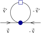
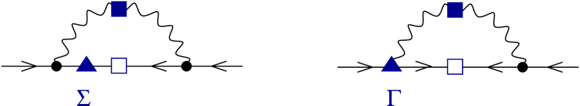
Figure 7: Higher order corrections to the gap equation in the high density effective theory.

The high density effective field theory enables us to perform a systematic expansion of the kernel of the gap equation in powers of the small scale and the coupling constant. It is not so obvious, however, how to solve the gap equation for more complicated kernels, and how the perturbative expansion of the kernel is related to the expansion of the solution of the gap equation.

For this purpose it is useful to develop a perturbative method for solving the gap equation [40, 19]. We can write the kernel of the gap equation as $K(x,y)=K_{0}(x,y)+\delta K(x,y)$, where $K_{0}(x,y)$ contains the leading IR divergence and $\delta K(x,y)$ is a perturbation. We expand both the gap function $\Delta(x)$ and the eigenvalue $x_{0}$ order by order $\delta K$,

$$\Delta(\bar{x}) = \Delta^{(0)}(\bar{x})+\Delta^{(1)}(\bar{x})+\Delta^{(2)}(\bar{x})+\ldots,$$ (38)

$$\bar{x}_{0} = \bar{x}_{0}^{(0)}+\bar{x}_{0}^{(1)}+\bar{x}_{0}^{(2)}+\ldots,$$ (39)

where we have defined $\bar{x}_{0}^{2}=g^{2}x_{0}^{2}/(18\pi^{2})$. The expansion coefficients can be found using the fact that the unperturbed solutions given in equ. (37) form an orthogonal set of eigenfunctions of $K_{0}$. The resulting expressions for $\bar{x}_{0}^{(i)}$ and $\Delta^{(i)}(\bar{x})$ are very similar to Rayleigh-Schroedinger perturbation theory. At first order we have

$$\bar{x}_{0}^{(1)} = -\frac{1}{2}\left(\bar{x}_{0}^{(0)}\right)^{2}\int_{0}^{1}d\bar{x}\int_{0}^{1}d\bar{y}\,$$ (40)

$$\hskip 42.67912pt\cdot\Delta_{0}^{(0)}(\bar{x})\delta\bar{K}(x_{0}\bar{x},x_{0}\bar{y})\Delta_{0}^{(0)}(\bar{y}),$$

$$c^{(1)}_{k} = \frac{\bar{x}_{0}^{(0)}}{1-\left(\frac{1}{2k+1}\right)^{2}}\int_{0}^{1}d\bar{x}\int_{0}^{1}d\bar{y}\,$$ (41)

$$\hskip 42.67912pt\cdot\Delta^{(0)}_{0}(\bar{x})\delta\bar{K}(x_{0}\bar{x},x_{0}\bar{y})\Delta^{(0)}_{k}(\bar{y}),$$

with $\Delta^{(1)}(x)=\sum c_{k}^{(1)}\Delta^{(0)}_{k}(x)$ and $\delta\bar{K}=g/(3\sqrt{2}\pi)\delta K$.

We can now study the role of various corrections to the kernel. The simplest contribution comes from collinear electric gluon exchanges and four-fermion operators. These terms do not change the shape of the gap function but give an $O(g)$ correction to the eigenvalue $\bar{x}_{0}$. This corresponds to a constant pre-exponential factor in the expression for the gap on the Fermi surface. An important advantage of the effective field theory method is that this factor is manifestly independent of the choice of gauge. The gauge independence of the pre-exponential factor is related to the fact that this coefficient is determined by four-fermion operators in the effective theory, and that these operators are matched on-shell.

The effect of the fermion wave function renormalization is slightly more complicated [40, 42]. Using equ. (30) we can write

$$\delta\bar{K}(x_{0}\bar{x},x_{0}\bar{y})=-\frac{g^{2}}{9\pi^{2}}\left(\bar{x}_{0}\bar{x}\right)K_{0}(x_{0}\bar{x},x_{0}\bar{y}).$$ (42)

The corresponding correction to the eigenvalue is

$$\bar{x}^{(1)}_{0}=-\frac{1}{2}\left(\bar{x}_{0}^{(0)}\right)^{2}\langle 0|\delta\bar{K}|0\rangle=\frac{4+\pi^{2}}{8}\frac{g}{3\sqrt{2}\pi},$$ (43)

where $\langle 0|\delta\bar{K}|0\rangle$ denotes the matrix element of the kernel between unperturbed gap functions, see equ. (40). At this order in $g$, there is no contribution from the quark-gluon vertex correction.

Note that the quark self energy correction makes an $O(g)$ correction to the kernel, even though it is an $O(g^{2})$ correction to the kernel. This is related to the logarithmic divergence in the self energy. The perturbative expansion of $\bar{x}_{0}$ is of the form

$$\bar{x}_{0}\sim g\log(\Delta)=O(g^{0})+O(g\log(g))+O(g)+\ldots.$$ (44)

Brown et al. argued that equ. (43) completes the $O(g)$ term. The result for the spin zero gap in the 2SC phase at this order is [20, 42, 19]

$$\Delta=512\pi^{4}\mu g^{-5}e^{-\frac{4+\pi^{2}}{8}}e^{-\frac{3\pi^{2}}{\sqrt{2}g}}.$$ (45)

In other spin or flavor channels the relevant four fermion operators are different and the pre-exponential factor is modified [20, 21, 22].

9 Very Low Energies

For momenta below the gap the dynamics is determined by Goldstone modes. In the CFL phase the effective lagrangian of the form [43]

$${\cal L}_{eff} = \frac{f_{\pi}^{2}}{4}{\rm Tr}\left[\partial_{0}\Sigma\partial_{0}\Sigma^{\dagger}-v_{\pi}^{2}\partial_{i}\Sigma\partial_{i}\Sigma^{\dagger}\right]+\Big{\{}B{\rm Tr}(M\Sigma^{\dagger})$$ (46)

$$\mbox{}+A_{1}\left[{\rm Tr}(M\Sigma^{\dagger})\right]^{2}+A_{2}{\rm Tr}\left[(M\Sigma^{\dagger})^{2}\right]$$

$$\mbox{}+A_{3}{\rm Tr}(M\Sigma^{\dagger}){\rm Tr}(M^{\dagger}\Sigma)+h.c.\Big{\}}+\ldots.$$

Here $\Sigma=\exp(i\phi^{a}\lambda^{a}/f_{\pi})$ is the chiral field, $f_{\pi}$ is the pion decay constant and $M$ is a complex mass matrix. The chiral field and the mass matrix transform as $\Sigma\to L\Sigma R^{\dagger}$ and $M\to LMR^{\dagger}$ under chiral transformations $(L,R)\in SU(3)_{L}\times SU(3)_{R}$. We have suppressed the singlet fields associated with the breaking of the exact $U(1)_{V}$ and approximate $U(1)_{A}$ symmetries. The coefficients $f_{\pi},B,A_{i}$ can be determined by matching the effective chiral lagrangian to the high density effective theory [44, 18, 14]

The chiral expansion has the structure

$${\cal L}\sim f_{\pi}^{2}\Delta^{2}\left(\frac{\vec{\partial}}{\Delta}\right)^{k}\left(\frac{\partial_{0}+MM^{\dagger}/p_{F}}{\Delta}\right)^{l}\left(\frac{MM}{p_{F}^{2}}\right)^{m}(\Sigma)^{n}(\Sigma^{\dagger})^{o}$$ (47)

Loop graphs are suppressed by powers of $p/(4\pi f_{\pi})$. Since the pion decay constant scale as $f_{\pi}\sim p_{F}$ loops are parametrically small as compared to higher order contact terms. The quark mass expansion is somewhat subtle because of the appearance of two scales, $m^{2}/p_{F}^{2}$ and $m^{2}/(p_{F}\Delta)$. This problem is discussed in more detail in [45].

10 Conclusions

In this contribution we discussed effective field theories in QCD at high baryon density. We focused, in particular, on the problem of power counting in the high density effective theory. We showed that the power counting is complicated by “hard dense loops”, i.e. loop diagrams that involve the large scale $\mu^{2}$. We proposed a modified power counting that takes these effects into account. The modified $l$ counting implies that hard dense loops in gluon $n$-point functions have to be resummed below the scale $g\mu$, and that four fermion operators are leading order in the HDET power counting. There are a number of important questions that remain to be addressed. An example is the renormalization of operators in the high density effective field theory.

Acknowledgments: We would like to thank I. Stewart for useful discussions. This work was supported in part by US DOE grant DE-FG-88ER40388.

References

- [1] D. Bailin and A. Love, Phys. Rept. 107, 325 (1984).
- [2] M. Alford, K. Rajagopal and F. Wilczek, Phys. Lett. B422, 247 (1998).
- [3] R. Rapp, T. Schäfer, E. V. Shuryak and M. Velkovsky, Phys. Rev. Lett. 81, 53 (1998).
- [4] M. Alford, K. Rajagopal and F. Wilczek, Nucl. Phys. B537, 443 (1999).
- [5] T. Schäfer, Nucl. Phys. B 575, 269 (2000).
- [6] K. Rajagopal and F. Wilczek, hep-ph/0011333.
- [7] M. Alford, Ann. Rev. Nucl. Part. Sci. 51, 131 (2001).
- [8] T. Schäfer, hep-ph/0304281.
- [9] D. H. Rischke, nucl-th/0305030.
- [10] D. K. Hong, Phys. Lett. B 473, 118 (2000).
- [11] D. K. Hong, Nucl. Phys. B 582, 451 (2000).
- [12] S. R. Beane and P. F. Bedaque, Phys. Rev. D 62, 117502 (2000).
- [13] S. R. Beane, P. F. Bedaque and M. J. Savage, Phys. Lett. B 483, 131 (2000).
- [14] T. Schäfer, Phys. Rev. D 65, 074006 (2002).
- [15] R. Casalbuoni, R. Gatto, M. Mannarelli and G. Nardulli, Phys. Lett. B 524, 144 (2002).
- [16] G. Nardulli, Riv. Nuovo Cim. 25N3, 1 (2002).
- [17] S. Hands, hep-ph/0310080.
- [18] T. Schäfer, Phys. Rev. D 65, 094033 (2002).
- [19] T. Schäfer, Nucl. Phys. A, in press (2003), [hep-ph/0307074].
- [20] W. E. Brown, J. T. Liu and H. c. Ren, Phys. Rev. D 62, 054016 (2000).
- [21] T. Schäfer, Phys. Rev. D 62, 094007 (2000).
- [22] A. Schmitt, Q. Wang and D. H. Rischke, Phys. Rev. D 66, 114010 (2002).
- [23] M. E. Luke, A. V. Manohar and I. Z. Rothstein, Phys. Rev. D 61, 074025 (2000).
- [24] C. W. Bauer, D. Pirjol and I. W. Stewart, Phys. Rev. D 66, 054005 (2002).
- [25] E. Braaten and R. D. Pisarski, Phys. Rev. D 45, 1827 (1992).
- [26] E. Braaten, Can. J. Phys. 71, 215 (1993).
- [27] R. Shankar, Rev. Mod. Phys. 66, 129 (1994).
- [28] J. Polchinski, hep-th/9210046.
- [29] B. Vanderheyden and J. Y. Ollitrault, Phys. Rev. D 56, 5108 (1997).
- [30] W. E. Brown, J. T. Liu and H. c. Ren, Phys. Rev. D 62, 054013 (2000).
- [31] C. Manuel, Phys. Rev. D 62, 076009 (2000).
- [32] C. Manuel, Phys. Rev. D 62, 114008 (2000).
- [33] D. Boyanovsky and H. J. de Vega, Phys. Rev. D 63, 034016 (2001).
- [34] T. Holstein, A. E. Norton, P. Pincus, Phys. Rev. B8, 2649 (1973).
- [35] M. Yu. Reizer, Phys. Rev. B 40, 11571 (1989).
- [36] A. Ipp, A. Gerhold and A. Rebhan, hep-ph/0309019.
- [37] D. T. Son, Phys. Rev. D 59, 094019 (1999).
- [38] T. Schäfer and F. Wilczek, Phys. Rev. D60, 114033 (1999).
- [39] D. K. Hong, V. A. Miransky, I. A. Shovkovy and L. C. Wijewardhana, Phys. Rev. D61, 056001 (2000).
- [40] W. E. Brown, J. T. Liu and H. Ren, Phys. Rev. D61, 114012 (2000).
- [41] R. D. Pisarski and D. H. Rischke, Phys. Rev. D61, 074017 (2000).
- [42] Q. Wang and D. H. Rischke, Phys. Rev. D 65, 054005 (2002).
- [43] R. Casalbuoni and D. Gatto, Phys. Lett. B464, 111 (1999).
- [44] D. T. Son and M. Stephanov, Phys. Rev. D61, 074012 (2000).
- [45] P. F. Bedaque and T. Schäfer, Nucl. Phys. A697, 802 (2002).