Flipping $SU(5)$ Towards Five Dimensional Unification

Abstract

It is shown that embedding of flipped $SU(5)$ in a five-dimensional $SO(10)$ enables exact unification of the gauge coupling constants. The demand for the unification uniquely determines both the compactification scale and the cutoff scale. These are found to be $M_{C}\approx 5.5\times 10^{14}\,{\rm GeV}$ and $M_{*}\approx 1.0\times 10^{17}\,{\rm GeV}$ respectively. The theory explains the absence of $d=5$ proton-decay operators through the implementation of the missing partner mechanism. On the other hand, the presence of $d=6$ proton-decay operators points towards the bulk localization of the first and the second family of matter fields.

I Introduction

The main motivation for supersymmetry (SUSY), besides its ability to stabilize the Higgs mass against the radiative corrections, is the way it steers the gauge couplings, within the Minimal Supersymmetric Standard Model (MSSM), towards the unification at a very high energy scale ($M_{\rm GUT}$). Assuming this is not an accident but a signal for a new physics we are prompted not only to embrace the MSSM but to incorporate it into the grand unified theory (GUT) where the gauge unification represents a genuine prediction of the framework. Another genuine prediction of the true GUT is, of course, a proton decay. It turns out, however, that it is very problematic to build both realistic and simple SUSY GUT scheme and still preserve the exact gauge coupling unification. For example, the parameter space of the simplest of all such schemes, the minimal $SU(5)$ SUSY GUT, has been severely constrained by the experimental limits on proton lifetime Goto:1998qg ; Babu:1998ep ; Murayama:2001ur ; Bajc:2002bv ; Bajc:2002pg .

The crux of the problem is that the exact gauge unification requires threshold corrections. But to create these corrections one needs certain fields, responsible for the proton decay, to be too light compared to the existing experimental constraints unless an ad hoc tuning of parameters takes place Bajc:2002bv ; Bajc:2002pg . This problem was not so serious in the past since the low-energy values of the gauge couplings were not known well enough, leaving a lot of room for maneuvering. The situation has changed after the electroweak precision measurements and the improvements in measurements of the strong coupling constant. The error bars have simply become sufficiently small to prevent the exact unification without the help of the troublesome threshold corrections. So, the question of whether we can achieve the exact gauge unification in accord with the low-energy measurements in a natural manner within SUSY GUTs is something we have to address.

Among the fields that can improve on the gauge unification, via threshold corrections, are the familiar colored Higgsinos. These are the fields that are responsible for $d=5$ proton-decay operator. Therefore, one wants them light enough to generate the appropriate corrections but heavy enough to avoid violation of the experimental limits on proton lifetime. This, again, is an extremely difficult task. One can entirely avoid the need of satisfying these conflicting requirements by using a flipped $SU(5)$ group DeRujula:1980qc ; Georgi:1980pw ; Barr:1981qv which automatically explains the absence of $d=5$ operators through the implementation of the simplest possible form of the missing partner mechanism Derendinger:1983aj ; Antoniadis:1987dx . However, flipped $SU(5)$ gives up one of the most attractive features of grand unification, namely unification of gauge couplings, because it is based on the group $SU(5)\times U(1)$. [This is not to say that the exact unification is impossible within the four-dimensional flipped $SU(5)$. For the most recent considerations in this direction see Refs. Ellis:2002vk ; Nanopoulos:2002qk .] Embedding the flipped $SU(5)$ within an $SO(10)$ gauge group retrieves the gauge unification but spoils the missing partner mechanism.

The way out, as has been recently shown Barr:2002fb , is to embed the flipped $SU(5)$ within an $SO(10)$ group in five dimensions using the extra-dimensional framework à la Kawamura Kawamura:1999nj ; Kawamura:2000ev ; Kawamura:2000ir . In this way, at the four-dimensional level, the famous missing partners can still be missing and the doublet-triplet splitting can be achieved without the dangerous Higgsino-mediated proton decay. But, one might expect naively that the exact gauge unification is impossible due to the threshold corrections that originate from the towers of Kaluza-Klein (KK) modes that are inherent to the theories with the compactified extra-dimensions. This naive expectation turns out to be wrong. The five-dimensional theory, being non-renormalizable, must have a cutoff ($M_{*}$). Therefore, the number of KK modes that contribute is finite. This also makes the threshold corrections finite and calculable so that the exact unification cannot be excluded a priori.

This paper is devoted to the issues pertaining to the gauge coupling unification in the five-dimensional setting. We show, following the footsteps of Kim and Raby Kim:2002im , that it is possible to achieve the exact unification using an $\mathcal{N}=1$ supersymmetric $SO(10)$ model on an $S^{1}/(Z_{2}\times Z_{2}^{\prime})$ orbifold. The orbifold has two inequivalent fixed points, $O$ and $O^{\prime}$, identified by the action of $(Z_{2}\times Z_{2}^{\prime})$ twisting. On the point (brane) $O$ there will be an $SO(10)$ gauge symmetry while on the point (brane) $O^{\prime}$ there will be a flipped $SU(5)$ gauge symmetries. Both symmetries will be the leftovers of a bigger, $SO(10)$, bulk symmetry. The bulk contains, besides the vector supermultiplet, a pair of chiral hypermutiplets: ${\bf 10}_{1H}$ and ${\bf 10}_{2H}$. They give the Higgs fields of the MSSM: $\overline{{\bf 2}}$ and ${\bf 2}$. The orbifolding procedure also reduces the amount of the supersymmetry from $\mathcal{N}=1$ in five dimensions to $\mathcal{N}=1$ in four dimensions. To obtain the low-energy phenomenology of the Standard Model (SM) group $\mathcal{H}$ we break flipped $SU(5)$ on the $O^{\prime}$ brane by implementing the missing partner mechanism. This time, in contrast to the model presented in Ref. Barr:2002fb , we do the breaking with the chiral superfields that reside on the $O^{\prime}$ brane.

There are two models in the literature we are going to compare our results with that provide the exact gauge coupling unification in the five-dimensional $S^{1}/(Z_{2}\times Z_{2}^{\prime})$ setting. The common feature for both models is the placement of the multiplets that contain the Higgs fields and the gauge sector of the MSSM in the bulk. We briefly review these models in what follows.

• The first one is an $SU(5)$ model of Hall and Nomura Hall:2001pg ; Hall:2001xb ; Hall:2002ci . In their model Hall:2002ci the orbifolding yields an $SU(5)$ gauge symmetry on one brane and the SM gauge symmetry on the other. In addition, the orbifolding accomplishes the doublet-triplet splitting by assigning the odd parity to the triplet fields. There is no need for any extra Higgs breaking except for the usual electroweak one. For gauge coupling unification not to be spoiled by arbitrary non-universal contributions coming from the brane with the SM gauge symmetry Hall and Nomura have to invoke two requirements: (i) the couplings at the cutoff scale $M_{*}$ must enter a strong coupling regime; (ii) the dimension(s) of the bulk must be large enough (when expressed in terms of the fundamental scale, i.e. cutoff scale, of the theory). We adopt their requirements in our model, too.

• The second model is a variant of an $SO(10)$ model of Dermíšek and Mafi Dermisek:2001hp . Here, we just outline the features that are relevant for comparison with our work. Since the breaking of $SO(10)$ down to $\mathcal{H}$ demands the reduction of the group rank Hebecker:2001jb , the authors use an extra Higgs breaking. In the original version of Dermíšek and Mafi Dermisek:2001hp the breaking of $SO(10)$ down to $SU(5)$ takes place on the $SO(10)$ brane. The low-energy signature of the SM gauge group is then due to the intersection of the Pati-Salam and $SU(5)$. The subsequent analysis of the variant of their model proposed by Kim and Raby Kim:2002im demonstrated the feasibility of the gauge unification. The breaking, in Kim and Raby case, takes place on a Pati-Salam brane affecting only the gauge sector of the theory. [The orbifolding has already projected out the triplet partners by assigning them odd parity.] We adopt and extend their method of analysis to demonstrate the successful unification in our case. The reason behind the extension is that, in our case, the extra Higgs breaking affects not only the gauge sector but also the Higgs sector. Namely, the breaking is what makes the triplets heavy via missing partner mechanism. This, as it turns out, has significant consequences on the renormalization group equation (RGE) running of the gauge couplings as we demonstrate later.

In Section II we introduce our model and specify the mass spectrum of all the fields. We then proceed with the discussion on the gauge coupling RGE running in five-dimensional orbifold setting in Section III. This is where our two main results, the relevant beta coefficients and their RGE numerical analysis, are presented. Finally, we briefly conclude in Section IV.

II An SO(10) model

We present an $SO(10)$ supersymmetric model in five dimensions compactified on an $S^{1}/(Z_{2}\times Z^{\prime}_{2})$ orbifold. The orbifold is created after the fifth dimension, being the circle $S^{1}$ of radius $R$, gets compactified through the reflection $y\rightarrow-y$ under $Z_{2}$ and $y^{\prime}\rightarrow-y^{\prime}$ under $Z^{\prime}_{2}$, where $y^{\prime}=y+\pi R/2$. There are two fixed points, $O$ and $O^{\prime}$, that bound the physical space $y\in[0,\pi R/2]$ of the bulk. The point $O$ is referred to as the “visible brane” while point $O^{\prime}$ at $y^{\prime}=0$ is referred to as the “hidden brane”.

We assume that the bulk contains an $\mathcal{N}=1$ vector supermultiplet, a ${\bf 45}_{g}$ of $SO(10)$, and two chiral hypermultiplets, ${\bf 10}_{1H}+{\bf 10}_{2H}$. The vector supermultiplet decomposes into a vector multiplet $V$, which contains the gauge bosons $A_{\mu}$ and corresponding gauginos, and a chiral multiplet $\Sigma$ of $\mathcal{N}=1$ supersymmetry in four dimensions. Each hypermultiplet splits into two left-handed chiral multiplets $\Phi$ and $\Phi^{c}$, having opposite gauge quantum numbers. To reduce $\mathcal{N}=1$ supersymmetry in five dimensions to $\mathcal{N}=1$ supersymmetry in four dimensions we use the parity assignment under $Z_{2}$. To reduce the gauge symmetry from $SO(10)$ down to flipped $SU(5)\otimes U(1)$ on the hidden brane we use the parity assignment under $Z_{2}^{\prime}$. The bulk content of the model is

$${\bf 45}_{g} = V^{++}_{{\bf 24}^{0}}+V^{++}_{{\bf 1}^{0}}+V^{+-}_{{\bf 10}^{-4}}+V^{+-}_{\overline{{\bf 10}}^{4}}+\Sigma^{--}_{{\bf 24}^{0}}+\Sigma^{--}_{{\bf 1}^{0}}+\Sigma^{-+}_{{\bf 10}^{-4}}+\Sigma^{-+}_{\overline{{\bf 10}}^{4}},$$ (1a)

$${\bf 10}_{1H} = \Phi^{++}_{{\bf 5}_{1}^{-2}}+\Phi^{+-}_{\overline{{\bf 5}}_{1}^{2}}+\Phi^{c--}_{\overline{{\bf 5}}_{1}^{2}}+\Phi^{c-+}_{{\bf 5}_{1}^{-2}},$$ (1b)

$${\bf 10}_{2H} = \Phi^{+-}_{{\bf 5}_{2}^{-2}}+\Phi^{++}_{\overline{{\bf 5}}_{2}^{2}}+\Phi^{c-+}_{\overline{{\bf 5}}_{2}^{2}}+\Phi^{c--}_{{\bf 5}_{2}^{-2}},$$ (1c)

where the first (second) superscript denotes the parity assignment under $Z_{2}$ ($Z_{2}^{\prime}$) transformation. Only the fields with the $++$ parity contain Kaluza-Klein zero mode fields ($n=0$) that have no effective four-dimensional mass. The masses of all other modes become quantized in units of $1/R\equiv M_{C}$, where $M_{C}$ is the compactification scale. For example, all $+-$ and $-+$ parity states are actually the KK towers of states with masses $M_{C},3M_{C},\ldots,(2n+1)M_{C},\ldots$, where $n$ is the mode number.

We want to have the low-energy phenomenology that is described by the SM group $\mathcal{H}$. But, at this point, the brane $O$ feels the $SO(10)$ gauge symmetry while the brane $O^{\prime}$ feels the flipped $SU(5)$ gauge symmetry. One could introduce a pair of Higgses in the bulk, the ${\bf 16}_{H}$ and the $\overline{\bf 16}_{H}$, and use the parity assignment to project out all the states except a pair ${\bf 10}^{1}_{H}+\overline{{\bf 10}}^{-1}_{H}$ that is needed for the missing partner mechanism on the visible brane Barr:2002fb . Here, however, we pursue slightly different direction. Namely, noting that the minimal set of Higgses that breaks flipped $SU(5)$ down to $\mathcal{H}$ is a pair of Higgs fields, ${\bf 10}^{1}_{H}+\overline{{\bf 10}}^{-1}_{H}$, we posit their existence on the hidden brane. [Similar idea on using the minimal Higgs content within an $SU(5)$ model has been exploited in Ref. Hebecker:2001wq .] With these fields in place we specify the following brane localized entry of the superpotential:

$$\kappa\Big{[}\delta\big{(}y-\frac{\pi R}{2}\big{)}+\delta\big{(}y-\frac{3\pi R}{2}\big{)}\Big{]}\Big{[}\Phi^{++}_{{\bf 5}_{1}^{-2}}\,{\bf 10}^{1}_{H}\,{\bf 10}^{1}_{H}+\Phi^{++}_{\overline{{\bf 5}}_{2}^{2}}\,\overline{{\bf 10}}^{-1}_{H}\,\overline{{\bf 10}}^{-1}_{H}\Big{]},$$ (2)

where $\kappa$ represents the Yukawa coupling with the mass dimension -1/2. Clearly, by giving very large VEVs to the $({\bf 1},{\bf 1},0)$ components of ${\bf 10}^{1}_{H}$ and $\overline{{\bf 10}}^{-1}_{H}$, we allow the triplet partners of the doublets in $\Phi^{++}_{{\bf 5}_{1}^{-2}}$ and $\Phi^{++}_{\overline{{\bf 5}}_{2}^{2}}$ to get large masses through the mating with the triplets of ${\bf 10}^{1}_{H}$ and $\overline{{\bf 10}}^{-1}_{H}$ without disturbing the lightness of the doublets. This can be schematically depicted as Babu:1993we

$$\begin{array}[]{c@{\!\!\!\!\!}c@{\!\!\!\!\!}c|c@{\!\!\!\!\!}c@{\!\!\!\!\!}c}\left(\begin{array}[]{c}{\bf 3}\\ \overline{{\bf 2}}\end{array}\right)&\rule[13.51505pt]{45.5244pt}{1.42262pt}&\left(\begin{array}[]{c}\overline{{\bf 3}}\\ {\rm{\bf other}}\end{array}\right)&\left(\begin{array}[]{c}{\bf 3}\\ \overline{{\rm{\bf other}}}\end{array}\right)&\rule[13.51505pt]{45.5244pt}{1.42262pt}&\left(\begin{array}[]{c}\overline{{\bf 3}}\\ {\bf 2}\end{array}\right)\\ \parallel&&\parallel&\parallel&&\parallel\\ \Phi^{++}_{{\bf 5}_{1}^{-2}}&&{\bf 10}^{1}_{H}&\overline{{\bf 10}}^{-1}_{H}&&\Phi^{++}_{\overline{{\bf 5}}_{2}^{2}}\end{array}$$ (3)

where, for simplicity, $({\bf 3},{\bf 2},1/3)+({\bf 1},{\bf 1},0)\equiv{\rm{\bf other}}$, and $\overline{{\bf 3}}=(\overline{{\bf 3}},{\bf 1},2/3)$. Moreover, the symmetry breaking makes the states $({\bf 1},{\bf 1},0)$, $({\bf 3},{\bf 2},1/3)$, and $(\overline{{\bf 3}},{\bf 2},-1/3)$ from $V^{++}_{{\bf 24}^{0}}$ and $V^{++}_{{\bf 1}^{0}}$ of ${\bf 45}_{g}$ absorb the corresponding components of the brane Higgses to become massive, leaving unbroken $\mathcal{H}$ gauge symmetry behind. [See Table 1 for the decomposition of $SO(10)$ down to $\mathcal{H}$ via flipped $SU(5)$.]

Table 1: The decomposition of the three lowest lying representations of $SO(10)$ under the flipped $SU(5)$ group and the Standard Model gauge group.

$SO(10)$	$SU(5)\otimes U(1)$	$SU(3)_{c}\otimes SU(2)_{L}\otimes U(1)_{Y}$
	${\bf 24}^{0}$	$({\bf 1},{\bf 1},0)\oplus({\bf 1},{\bf 3},0)\oplus({\bf 3},{\bf 2},1/3)\oplus(\overline{{\bf 3}},\overline{{\bf 2}},-1/3)\oplus({\bf 8},{\bf 1},0)$
	${\bf 10}^{-4}$	$({\bf 1},{\bf 1},-2)\oplus(\overline{{\bf 3}},{\bf 1},-4/3)\oplus({\bf 3},\overline{{\bf 2}},-5/3)$
${\bf 45}$	$\overline{{\bf 10}}^{4}$	$({\bf 1},{\bf 1},2)\oplus({\bf 3},{\bf 1},4/3)\oplus(\overline{{\bf 3}},{\bf 2},5/3)$
	${\bf 1}^{0}$	$({\bf 1},{\bf 1},0)$
	${\bf 1}^{5}$	$({\bf 1},{\bf 1},2)$
${\bf 16}$	$\overline{{\bf 5}}^{-3}$	$({\bf 1},\overline{{\bf 2}},-1)\oplus(\overline{{\bf 3}},{\bf 1},-4/3)$
	${\bf 10}^{1}$	$({\bf 1},{\bf 1},0)\oplus(\overline{{\bf 3}},{\bf 1},2/3)\oplus({\bf 3},{\bf 2},1/3)$
	${\bf 5}^{-2}$	$({\bf 1},\overline{{\bf 2}},-1)\oplus({\bf 3},{\bf 1},-2/3)$
${\bf 10}$	$\overline{{\bf 5}}^{2}$	$({\bf 1},{\bf 2},1)\oplus(\overline{{\bf 3}},{\bf 1},2/3)$

In the discussion from the previous paragraph, we have glossed over a fact that the bulk fields are KK towers of states. The explicit brane localized breaking terms will disturb every state of that tower due to the change of the boundary conditions. Since we want to do an RGE analysis we need to determine the KK tower position, i.e. the mass, of every state after the disturbance has taken place. This is what we do next.

II.1 Mass Spectrum of the Gauge Fields

The five-dimensional theory is non-renormalizable. Therefore, we expect the theory to have a cutoff scale $M_{*}$ where some new physics comes into play (e.g. other dimensions beyond five, strings). We take the VEVs of the symmetry breaking Higgs fields to be of the order of this cutoff: $\langle({\bf 1},{\bf 1},0)\rangle\equiv M\sim M_{*}$. Then the Lagrangian involving the gauge fields gets additional contribution Nomura:2001mf ; Kim:2002im

$$\mathcal{L}\subset\frac{1}{2}\Big{[}\delta\big{(}y-\frac{\pi R}{2}\big{)}+\delta\big{(}y-\frac{3\pi R}{2}\big{)}\Big{]}g_{5}^{2}M^{2}A^{\hat{a}}_{\mu}A^{\hat{a}\mu},$$ (4)

where $g_{5}^{2}$ represents the gauge coupling of the five-dimensional theory and $\hat{a}$ is an $SO(10)$ group index that goes through all the gauge fields associated with the broken $++$ parity generators we mentioned at the end of Section II. [The five-dimensional gauge coupling $g_{5}^{2}$ has mass dimension $-1$.] The equations of motion for the “broken” gauge bosons are Nomura:2001mf ; Kim:2002im

$$-\partial_{y}^{2}A^{\hat{a}}_{\mu}(x,y)+\Big{[}\delta\big{(}y-\frac{\pi R}{2}\big{)}+\delta\big{(}y-\frac{3\pi R}{2}\big{)}\Big{]}g_{5}^{2}M^{2}A^{\hat{a}}_{\mu}(x,y)=(M^{A}_{n})^{2}A^{\hat{a}}_{\mu}(x,y),$$ (5)

where $M^{A}_{n}$ represents the effective Kaluza-Klein mass in four dimensions of the $n$th mode. It is defined via Klein-Gordon equation $\big{[}\partial_{\nu}\partial^{\nu}+(M^{A}_{n})^{2}\big{]}A^{\hat{a}}_{\mu}(x,y)=0$. The second term on the left-hand side of Eq. (5) is responsible for the deviation from the usual mass spectrum of the $++$ parity fields ($M^{A}_{n}=0,2M_{C},\ldots,2nM_{C},\ldots$). It reminds us of the delta function-type potential in ordinary Schrödinger’s equation. The role of this term is thus to repel the bulk field wave function away from the brane. In the language of the effective four-dimensional theory this means that even the zero mode ($n=0$) of the gauge bosons becomes massive. Taking the following ansatz for the five-dimensional gauge field on the segment $y\in[0,\pi R/2]$:

$$A^{\hat{a}}_{\mu}(x,y)=\frac{1}{\sqrt{\pi R}}\sum^{\infty}_{n=0}N_{n}A^{\hat{a}(n)}_{\mu}(x)\cos M_{n}^{A}y,$$ (6)

the eigenvalue equation for the effective mass, due to the nontrivial boundary condition at the hidden brane, takes the form Nomura:2001mf

$$\tan\frac{M_{n}^{A}\pi R}{2}=\frac{g_{5}^{2}M^{2}}{2M_{n}^{A}}.$$ (7)

The normalization constant for the $++$ parity bulk fields also changes from $1/\sqrt{2^{\delta_{n0}}}$ to $N_{n}=\big{[}1+M_{C}g_{5}^{2}M^{2}\cos^{2}\frac{M_{n}^{A}\pi R}{2}/(\pi(M_{n}^{A})^{2})\big{]}^{-1/2}$ Choi:2003bh . The plot of the modified wave function profile for $n=1$ is given in Fig. 1. [We excluded the normalization constants for simplicity.]

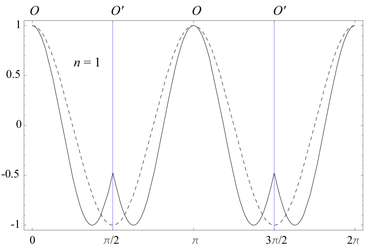
Figure 1: A plot of an $n=1$ mode of the bulk field wave function profile in the fifth dimension. The dashed line represents undisturbed profile given by $\cos 2ny$. The solid line represents the profile after the perturbation due to the boundary condition is accounted for. The radius $R$ is taken to be 1.

There are two interesting approximations that we can consider: $g_{5}^{2}M^{2}\gg M_{n}^{A}$ and $g_{5}^{2}M^{2}\ll M_{n}^{A}$. The former one generates the following approximate solution of the eigenvalue equation for the mass spectrum

$$M_{n}^{A}\simeq(2n+1)M_{C}\big{[}1-\varepsilon+\varepsilon^{2}\big{]},$$ (8)

while the latter one yields

$$M_{0}^{A}\simeq 2M_{C}\sqrt{\frac{1}{\pi^{2}\varepsilon}},\;\;\mbox{and}\;\;M_{n\neq 0}^{A}\simeq 2nM_{C}\big{[}1+\frac{1}{\pi^{2}\varepsilon n^{2}}\big{]},$$ (9)

where we define $\varepsilon\equiv(4M_{C})/(\pi g_{5}^{2}M^{2})$. The two approximations generate qualitatively different mass spectra. Therefore, it is very important to determine which one is applicable to our scenario. Assuming that all the couplings of the theory enter the strong regime at the cutoff $M_{*}$ we can use the result of the naive dimensional analysis Chacko:1999hg in higher dimensional theories that suggests $g_{5}^{2}\simeq 24\pi^{3}/M_{*}$ and $M\simeq M_{*}/(4\pi)$, which gives $g_{5}^{2}M^{2}\simeq 3/2\pi M_{*}>M_{*}\gg M_{n}^{A}$. We thus choose the former approximation. Following the work of Kim and Raby Kim:2002im , we introduce the parameter $\zeta=2N\varepsilon$, where $2N=M_{*}/M_{C}$ and $\zeta\simeq 8/(3\pi^{2})\simeq 0.27$, to rewrite the approximate mass spectrum of the broken gauge bosons as

$$M_{n}^{A}\simeq M_{C}\big{(}2n+1-\frac{n}{N}\zeta\big{)}.$$ (10)

One interesting feature to note is that the boundary condition in Eq. (7) is not absolute Nomura:2001mf . In our case, the broken $++$ parity field modes start off with the mass spectrum that mimics the spectrum of the $+-$ and $-+$ parity field modes but then gradually merges with the spectrum of undisturbed $++$ and $--$ parity bulk fields as one moves up the Kaluza-Klein tower of states. One should also keep in mind that the supersymmetry ensures the same fate for the chiral partners $\Sigma$ of the vector fields $V$. Namely, the mass spectrum of the fields in $\Sigma^{--}$ are shifted in the same manner as the states in the $V^{++}$ that are made massive through the brane gauge breaking. With that said, we turn to the consideration of the Higgs field mass spectrum.

II.2 Mass Spectrum of the Higgs Fields

The missing partner mechanism affects only the color triplets of the bulk states with $++$ and $--$ parities. To determine their effective mass spectrum we concentrate on the masses of the color Higgsinos. Supersymmetry then ensures the same mass spectrum for their bosonic partners. Moreover, since there are two separate color triplet sectors, as indicated by the vertical line in Eq. (3), we treat only one of them. The other sector will have the same mass spectrum as long as both sectors share the same dimensionful coupling $\kappa$. We assume this to be the case. Note that the bulk states with the $+-$ and $-+$ parities, i.e. the odd states, do not get affected by the brane breaking.

To make the discussion as transparent as possible we adopt the following notation for the triplet Higgsinos: $H_{C}\in\Phi^{++}_{{\bf 5}_{1}^{-2}}$, $H_{C}^{c}\in\Phi^{c--}_{\overline{{\bf 5}}_{1}^{2}}$, and $H_{\overline{C}_{H}}\in{\bf 10}^{1}_{H}$. Their equations of motion, derived from the brane coupling term in Eq. (2) and the bulk action (see Arkani-Hamed:2001tb ), read Choi:2003bh

$${\rm i}{\bar{\sigma}}^{\mu}\partial_{\mu}H_{\overline{C}_{H}}-\kappa M\overline{H}_{C}|_{y=(\pi R/2,\,3\pi R/2)}=0,$$ (11)

$${\rm i}{\bar{\sigma}}^{\mu}\partial_{\mu}H_{C}-\partial_{y}\overline{H}^{c}_{C}-\kappa M\overline{H}_{\overline{C}_{H}}\big{(}\delta(y-\pi R/2)+\delta(y-3\pi R/2)\big{)}=0,$$ (12)

$${\rm i}{\bar{\sigma}}^{\mu}\partial_{\mu}H^{c}_{C}+\partial_{y}\overline{H}_{C}=0.$$ (13)

These equations are satisfied by the following ansatz for the five-dimensional Higgsino fields on the segment $y\in[0,\pi R/2]$

$$H_{C}(x,y) =\frac{1}{\sqrt{\pi R}}\sum_{n}N^{H_{C}}_{n}h^{(n)}_{1}(x)\cos M^{H_{C}}_{n}y,$$ (14)

$$H^{c}_{C}(x,y) =\frac{1}{\sqrt{\pi R}}\sum_{n}N^{H_{C}}_{n}h^{(n)}_{2}(x)\sin M^{H_{C}}_{n}y,$$ (15)

and the Higgsino field localized on the hidden brane

$$H_{\overline{C}_{H}}(x) =\frac{1}{\sqrt{\pi R}}\sum_{n}N^{H_{C}}_{n}\frac{\kappa M}{M^{H_{C}}_{n}}h^{(n)}_{2}(x)\cos\frac{M^{H_{C}}_{n}\pi R}{2}.$$ (16)

Here, the eigenvalue equation for the effective mass, due to the nontrivial boundary condition at the hidden brane, takes the form Choi:2003bh

$$\tan\frac{M_{n}^{H_{C}}\pi R}{2}=\frac{\kappa^{2}M^{2}}{2M_{n}^{H_{C}}},$$ (17)

where we define the effective KK mass via a pair of Weyl equations: ${\rm i}{\bar{\sigma}}^{\mu}\partial_{\mu}h^{(n)}_{1}=M^{H_{C}}_{n}{\overline{h}}^{(n)}_{2}$ and ${\rm i}{\bar{\sigma}}^{\mu}\partial_{\mu}h^{(n)}_{2}=M^{H_{C}}_{n}{\overline{h}}^{(n)}_{1}$.

The naive dimensional analysis Chacko:1999hg in the strong coupling regime yields $\kappa\simeq(24\pi^{3}/M_{*})^{1/2}$, which implies that $\kappa^{2}M^{2}(\simeq g_{5}^{2}M^{2})\gg M^{H_{C}}_{n}$. In this limit, the mass spectrum of the Higgsino triplets looks, in form, exactly the same as the mass spectrum of the broken gauge fields. Namely, the mass eigenvalues of Eq. (17) are

$$M_{n}^{H_{C}}\simeq M_{C}\big{(}2n+1-\frac{n}{N}\zeta\big{)},$$ (18)

where we assume that $\kappa^{2}M^{2}=g_{5}^{2}M^{2}$ for simplicity. For completeness, the normalization constant $N_{n}^{H_{C}}$ is Choi:2003bh

$$N^{H_{C}}_{n}=\bigg{(}1+\frac{M_{C}\kappa^{2}M^{2}}{\pi(M^{H_{C}}_{n})^{2}}\cos^{2}\frac{M^{H_{C}}_{n}\pi R}{2}\bigg{)}^{-1/2}.$$ (19)

In the case of the color Higgsinos there is a mixing between the bulk and the brane fields. It is the role of the brane field $H_{\overline{C}_{H}}$ to give the mass to the zero mode component of $H_{C}$. As described in Ref. Choi:2003bh , the Weyl spinors, $h_{1}^{(n)}$ and $h_{2}^{(n)}$, pair up at every Kaluza-Klein level to obtain the Dirac mass. The remaining states in the ${\bf 10}^{1}_{H}$ of Higgs get absorbed by the broken gauge bosons and completely disappear as far as the running is concerned. We show the mass spectrum of one part of the Higgs sector in Fig. 2. The other part looks exactly the same.

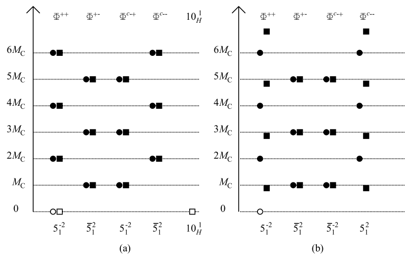
Figure 2: (a) A mass spectrum of the Kaluza-Klein towers of the Higgs sector after the compactification, but before the brane localized breaking. (b) The mass spectrum after the brane localized breaking. The circles represent the doublets and the squares represent the triplets.

Since this concludes the discussion on the mass spectrum of both the gauge and the Higgs fields we turn our attention towards the RGE analysis.

III Kaluza-Klein unification

The running of the gauge couplings in our model is the same as the running in the usual four-dimensional theory as long as we stay below the compactification scale $M_{C}$. But, once we venture over $M_{C}$, the running is affected by the towers of Kaluza-Klein states until we reach the cutoff scale $M_{*}$, which we define as the scale where effective gauge couplings merge. Since there are numerous states in the KK towers one might expect that the analysis of the threshold effects on the gauge coupling running from $M_{C}$ to $M_{*}$ is very difficult even at a one-loop level. This, however, is not the case as we show next.

Let us, for concreteness, limit our discussion to the five-dimensional theory that is based on the simple gauge group $\mathcal{F}$. The main simplification originates from the observation that the compactification procedure forces all the states that make up a single representation of $\mathcal{F}$ to appear within the interval $[2nM_{C},2(n+1)M_{C}]$ for every $n\neq 0$. [This statement is true regardless of the type of the additional brane boundary conditions we discussed in the previous two sections.] These states obviously contribute in an $\mathcal{F}$ invariant way to the running of all the gauge coupling constants after we go over $2(n+1)M_{C}$. Thus, the contribution of the $n$th Kaluza-Klein level that starts to appear at $2nM_{C}$ drops out of the running of the difference of the gauge couplings after we reach $2(n+1)M_{C}$. In view of this fact we are motivated to pursue the differential running, i.e. the running of the difference of the gauge couplings. The previous observation also implies that the beta coefficients reset themselves to the values of the familiar coefficients of the Standard Model group $\mathcal{H}$ every time we go over another $2(n+1)M_{C}$ scale.

Nontrivial boundary conditions distort the spectrum of Kaluza-Klein masses. In our case, the members of the $n$th mode emerge at $2nM_{C}$, $(2n+1-\frac{n}{N}\zeta)M_{C}$, $(2n+1)M_{C}$, and $(2n+2)M_{C}$ energy levels. We have already concluded that from $2nM_{C}$ to $(2n+1-\frac{n}{N}\zeta)M_{C}$ the beta coefficients must be the coefficients of the SM group $\mathcal{H}$. We call this region I. Region II is the region from $(2n+1-\frac{n}{N}\zeta)M_{C}$ to $(2n+1)M_{C}$, while region III stretches from $(2n+1)M_{C}$ to $(2n+2)M_{C}$ for $n\neq 0$. The notation here and in what follows is exactly the same as the notation of Kim and Raby Kim:2002im . Note that we do not mention the matter fields at any point. The reason is that the matter fields of one family contribute equally to the running of the gauge couplings regardless of their origin, i.e. whether they are located in the bulk or on the brane.

As shown by Kim and Raby Kim:2002im , if the compactification breaks $\mathcal{F}$ to $\mathcal{G}$ and, then, the brane breaking reduces $\mathcal{G}$ to the SM group $\mathcal{H}$, the beta coefficients of the gauge sector are:

$$\begin{split}b^{\rm I}_{\rm gauge}&=b^{\mathcal{H}}(V);\\ b^{\rm II}_{\rm gauge}&=b^{\mathcal{H}}(V)+b^{\mathcal{G/H}}(V)+b^{\mathcal{G/H}}(\Sigma)=b^{\mathcal{G}}(V)+b^{\mathcal{G}}(\Sigma)-b^{\mathcal{H}}(\Sigma);\\ b^{\rm III}_{\rm gauge}&=b^{\mathcal{H}}(V)+b^{\mathcal{G/H}}(V)+b^{\mathcal{G/H}}(\Sigma)+b^{\mathcal{F/G}}(V)+b^{\mathcal{F/G}}(\Sigma)=-b^{\mathcal{H}}(\Sigma).\end{split}$$ (20)

[The notation is that $b\equiv(b_{1},b_{2},b_{3})$, where $b_{1}$, $b_{2}$, and $b_{3}$ are the coefficients associated with the gauge couplings of $U(1)_{Y}$, $SU(2)_{L}$, and $SU(3)_{c}$ respectively.] Here, we use the fact that $b^{\mathcal{F}}(V)\equiv b^{\mathcal{H}}(V)+b^{\mathcal{G/H}}(V)+b^{\mathcal{F/G}}(V)$ is an $\mathcal{F}$ invariant coefficient that drops out from the running of the differences of the gauge couplings. The same statement holds for $b^{\mathcal{F}}(\Sigma)\equiv b^{\mathcal{H}}(\Sigma)+b^{\mathcal{G/H}}(\Sigma)+b^{\mathcal{F/G}}(\Sigma)$ coefficient. $\mathcal{G/H}$ and $\mathcal{F/G}$ represent the appropriate coset-spaces (e.q. states that are in $\mathcal{G}\supset\mathcal{H}$ but not in $\mathcal{H}$ belong to $\mathcal{G/H}$). Note that we always have $b(\Sigma)=-b(V)/3$ since $\Sigma$ is the chiral superfield and $V$ is the vector superfield. In our case $\mathcal{F}$ corresponds to $SO(10)$ and $\mathcal{G}$ corresponds to the flipped $SU(5)$ group.

Before we consider the beta coefficient of the Higgs sector we note the following: the beta coefficients of the two supersymmetric Higgs doublets (triplets) are $b({\bf 2})\equiv(3/5,1,0)$ ($b({\bf 3})\equiv(2/5,0,1)$). Therefore, the sum of the contributions of the pair of doublets and the pair of triplets does not affect the differential running and can be freely discarded. Moreover, as far as the differential running is concerned, we can write $b({\bf 2})=-b({\bf 3})=(0,2/5,-3/5)$, where we subtract the overall constant to make $b_{1}=0$. This we do with all the other beta coefficients in what follows. Recalling that there are two Higgs sectors we can write:

$$\begin{split}b^{\rm I}_{\rm Higgs}&=b({\bf 2});\\ b^{\rm II}_{\rm Higgs}&=b({\bf 2})+2b({\bf 3})=b({\bf 3});\\ b^{\rm III}_{\rm Higgs}&=b({\bf 3})+2b({\bf 2})+2b({\bf 3})=b({\bf 3}).\end{split}$$ (21)

Finally, we are ready to analyze the running at one-loop level. The relevant RGEs and all the definitions are taken from Kim and Raby Kim:2002im . We present them here for completeness of this work. The one-loop RGEs for the gauge couplings in the effective four-dimensional theory are

$$\frac{2\pi}{\alpha_{i}(\mu)}=\frac{2\pi}{\alpha(M_{*})}+\big{[}b^{\mathcal{H}}_{i}(V)+b^{\mathcal{H}}_{i}({\bf 2})+b^{\mathcal{H}}_{\rm matter}\big{]}\ln\frac{M_{C}}{\mu}+\Delta^{\rm Higgs}_{i}+\Delta^{\rm gauge}_{i},$$ (22)

where $\Delta$’s describe the appropriate threshold corrections of the Kaluza-Klein modes from $M_{C}$ to $M_{*}$. They are given by

$$\Delta\equiv\ b^{\rm eff}\ln\frac{M_{*}}{M_{C}}=b^{\rm I}A_{\rm I}+b^{\rm II}A_{\rm II}+b^{\rm III}A_{\rm III},$$ (23)

with

$$A_{\rm I} = \sum_{n=1}^{N-1}\ln\frac{2n+1-\frac{n}{N}\zeta}{2n},$$ (24a)

$$A_{\rm II} = \sum_{n=1}^{N-1}\ln\frac{2n+1}{2n+1-\frac{n}{N}\zeta},$$ (24b)

$$A_{\rm III} = \sum_{n=1}^{N}\ln\frac{2n}{2n-1}.$$ (24c)

Obviously, $A_{\rm I}$, $A_{\rm II}$ and $A_{\rm III}$ allow us to sum over the threshold corrections from the corresponding regions.

Taking the large $N$ limit, where $2N=M_{*}/M_{C}$, and using the approximation $\ln(1+x)=x+\cdots$, Kim and Raby Kim:2002im give the following expression for the threshold corrections of the gauge and the Higgs sector:

$$\Delta=\frac{1}{2}(b^{\rm III}+b^{I})\ln\frac{M_{*}}{M_{C}}+\frac{1}{2}(b^{\rm III}-b^{\rm I})\ln\frac{\pi}{2}+\frac{1}{2}(b^{\rm II}-b^{\rm I})\zeta.$$ (25)

Looking back at Eqs. (20) and (21) we have for our model

$$\Delta^{\rm gauge} = \frac{2}{3}b^{\mathcal{H}}(V)\ln\frac{M_{*}}{M_{C}}-\frac{1}{3}b^{\mathcal{H}}(V)\ln\frac{\pi}{2}+\frac{1}{3}\big{[}b^{\mathcal{G}}(V)-b^{\mathcal{H}}(V)\big{]}\zeta,$$ (26a)

$$\Delta^{\rm Higgs} = -b({\bf 2})\ln\frac{\pi}{2}-b({\bf 2})\zeta.$$ (26b)

Moreover, since $b^{\mathcal{H}}(V)$ represents the beta coefficients of the gauge sector of the MSSM we have $b^{\mathcal{H}}(V)=(0,-6,-9)$. On the other hand, $b^{\mathcal{G}}(V)$ represents the beta coefficients of the gauge sector of the supersymmetric flipped $SU(5)$: ${\bf 24}^{0}+{\bf 1}^{0}$. Therefore, $b^{\mathcal{G}}(V)=(-3/5,-15,-15)\equiv(0,-72/5,-72/5)$, where we again subtract the overall constant contribution to make $b_{1}$ coefficient equal to zero. Using these results we find:

$$\Delta^{\rm gauge} = \big{(}0,-4\ln\frac{M_{*}}{M_{C}}+2\ln\frac{\pi}{2}-\frac{14}{5}\zeta,-6\ln\frac{M_{*}}{M_{C}}+3\ln\frac{\pi}{2}-\frac{9}{5}\zeta\big{)},$$ (27a)

$$\Delta^{\rm Higgs} = \big{(}0,-\frac{2}{5}\ln\frac{\pi}{2}-\frac{2}{5}\zeta,\frac{3}{5}\ln\frac{\pi}{2}+\frac{3}{5}\zeta\big{)}.$$ (27b)

Our goal is to find the values of $M_{C}$ and $M_{*}$ that allow the exact unification, at least at one-loop level, of the gauge coupling constants at the scale $M_{*}$. To be able to do that we first recall the situation we have in the usual four-dimensional SUSY GUT. There we define $M_{\rm GUT}$ to be the scale where $\alpha_{1}(M_{\rm GUT})=\alpha_{2}(M_{\rm GUT})\equiv\tilde{\alpha}_{\rm GUT}$ Kim:2002im with the running given by

$$\frac{2\pi}{\alpha_{i}(\mu)}=\frac{2\pi}{\alpha_{i}(M_{\rm GUT})}+\big{[}b^{\mathcal{H}}_{i}(V)+b^{\mathcal{H}}_{i}({\bf 2})+b^{\mathcal{H}}_{\rm matter}\big{]}\ln\frac{M_{\rm GUT}}{\mu}.$$ (28)

If we ask how far off from $\tilde{\alpha}_{\rm GUT}$ the coupling $\alpha_{3}(M_{\rm GUT})$ is, and parameterize the degree of nonunification via $\delta_{3}=\big{(}2\pi/\alpha_{3}(M_{\rm GUT})-2\pi/\tilde{\alpha}_{\rm GUT}\big{)}$, we obtain $5\lesssim\delta_{3}\lesssim 6$ depending on the exact spectrum of SUSY particles. We show one example of differential running in Fig. 3. This example takes into the account not only the one-loop but the two-loop effects on the running of the gauge couplings. We also assume that the superpartners have masses of the order of $m_{t}$, and take the lower experimental limit $\tan\beta=3$ :2001xx .

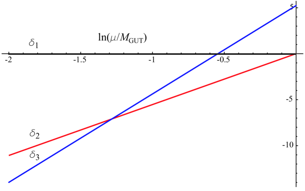
Figure 3: A plot of the differential running $\delta_{i}(\mu)=2\pi(1/\alpha_{i}(\mu)-1/\alpha_{1}(\mu))$ versus $\ln(\mu/M_{\rm GUT})$, where $M_{\rm GUT}=2.37\times 10^{16}$ GeV.

In the five-dimensional setting the deviation from the usual running starts at $M_{C}$ scale. Therefore, at $M_{C}$, the left-hand sides of Eqs. (22) and (28) must be the same. Thus, we have that

$$\begin{split}\delta_{2}(M_{C})&=\big{[}b^{\mathcal{H}}_{2}(V)+b^{\mathcal{H}}_{2}({\bf 2})]\ln\frac{M_{\rm GUT}}{M_{C}}=\Delta^{\rm gauge}_{2}+\Delta^{\rm Higgs}_{2},\\ \delta_{3}(M_{C})&=\big{(}2\pi/\alpha_{3}(M_{\rm GUT})-2\pi/\tilde{\alpha}_{\rm GUT}\big{)}\\ &\quad+\big{[}b^{\mathcal{H}}_{3}(V)+b^{\mathcal{H}}_{3}({\bf 2})]\ln\frac{M_{\rm GUT}}{M_{C}}=\Delta^{\rm gauge}_{3}+\Delta^{\rm Higgs}_{3}.\end{split}$$ (29)

Solving these equations yields

$$M_{C}\approx 5.5\times 10^{14}\,{\rm GeV},\,\,\mbox{and}\,\,M_{*}\approx 1.0\times 10^{17}\,{\rm GeV},$$ (30)

where we use the same value of $\delta_{3}$ as is used by Kim and Raby Kim:2002im ($\delta_{3}\simeq 6$) and we take the corresponding value of $M_{\rm GUT}$ ($M_{\rm GUT}=3\times 10^{16}$ GeV). These values imply that $N=90$, justifying the large $N$ approximations. This also ensures that the effect of the non-universal brane kinetic terms, present on the $O^{\prime}$ brane, on the gauge coupling unification is sufficiently small to be neglected Hall:2001pg .

In view of our results the following picture emerges. The effective theory below the compactification scale looks exactly the same as the usual MSSM theory. Then, once we go above $M_{C}$, there emerge the towers of the Kaluza-Klein states that change the behavior of the gauge running through the set of small but numerous threshold corrections. The theory finally yields the gauge unification at $M_{*}>M_{\rm GUT}$ where all the couplings of the theory enter the strong regime. At that point the five-dimensional theory must be embedded into more fundamental physical picture.

We should note that our result is not very sensitive to the exact value of the small parameter $\zeta$. On the other hand, the values of $M_{C}$ and $M_{*}$ depend very strongly on the value of $\delta_{3}$. We have taken $\delta_{3}\simeq 6$ to be able to compare our results with the analysis of Kim and Raby Kim:2002im . This value, coming from the RGE propagation of the experimental value of $\alpha_{3}(m_{Z})=0.118\pm 0.003$ Hagiwara:fs from the $m_{Z}$ scale to the GUT scale, could be reduced in near future. Namely, the new estimate of $\alpha_{3}$ from $\tau$ lifetime suggests $\alpha_{3}(m_{Z})=0.1221^{+0.0026}_{-0.0023}$ Erler:2002bu ; Langacker:2003tv . This would have a large impact on our result since the corresponding value of $\delta_{3}$ ($\delta_{3}\simeq 3$) would imply $N=2$, making the whole KK unification picture questionable. The model of Kim and Raby Kim:2002im for the case of $\delta_{3}\simeq 3$ yields $N=27$.

This paper is devoted solely to the analysis of the gauge coupling unification. This means that there are many questions left unanswered. For example, one might ask what mechanism breaks four-dimensional $\mathcal{N}=1$ supersymmetry. Or, how the Higgs fields responsible for the missing partner mechanism get their VEVs. Our intention was not to answer the questions like these but to demonstrate the possibility of the five-dimensional Kaluza-Klein unification and this we did. But, some of these questions, including the possibility of having a model with the realistic mass patterns, have already been tackled in Ref. Barr:2002fb . [There are, of course, different directions one might take. Namely, a number of five-dimensional $SO(10)$ models with the Pati-Salam signature on one brane and $SO(10)$ signature on the other brane has been studied in the literature Dermisek:2001hp ; Albright:2002pt ; Kyae:2002ss ; Kim:2002im ; Kim:2003vr . Even the most general scenario of having a model with the five-dimensional $SO(10)$ gauge symmetry that is broken by compactification on both branes has also been investigated recently Kyae:2003ek .]

Our result for $M_{C}$ and $M_{*}$ is very similar to the result obtained by Kim and Raby Kim:2002im . This is due to the fact that the biggest correction to the standard four-dimensional running in both cases comes from the first term in Eq. (26a). Since this term involves the beta coefficients of the SM gauge group only, the leading corrections must be the same for all the schemes with the realistic low-energy signature. The main difference between the two models in the gauge sector is generated by the beta coefficients $b^{\mathcal{G}}(V)$ of the gauge group on the hidden brane. In our case the hidden brane has the flipped $SU(5)$ group with $b^{\mathcal{G}}(V)=(0,-72/5,-72/5)$, while in the case of Kim and Raby the hidden brane harbors PS gauge group with $b^{\mathcal{G}}(V)=(0,12/5,-18/5)$. The main difference in the Higgs sector stems from the fact that there is no distinction between the region I and region II in Kim and Raby case since the additional boundary conditions do not affect the Higgs sector at all. Therefore, the second term in Eq. (26b) is absent in their case. It is interesting to note that the difference between the two models is in the terms that are proportional to the small parameter $\zeta$. Therefore, the limit $\zeta\rightarrow 0$ gives the same result in both cases. In that limit we obtain $M_{C}\approx 3.2\times 10^{14}\,{\rm GeV}$, and $M_{*}\approx 2.2\times 10^{17}\,{\rm GeV}$. Interestingly enough, the same limit reproduces the results of the analysis on the gauge coupling unification of the five-dimensional $SU(5)$ model Hall:2002ci . One can even make a more general statement about various models yielding the same result in the limit when the brane breaking is large enough ($\zeta\rightarrow 0$). Namely, one expects the same corrections to the usual four-dimensional running in all models that fulfill the following conditions: i) $\mathcal{F}$ is a unified group; ii) $\mathcal{H}$ corresponds to the SM group; iii) Symmetry breaking $\mathcal{G}\rightarrow\mathcal{H}$ is localized at the $\mathcal{G}$ brane; iv) the MSSM Higgses originate from the bulk. Clearly, all of the above conditions are satisfied by the models we consider.

Even though the exact unification of the gauge couplings in the four-dimensional flipped $SU(5)$ cannot be excluded Ellis:2002vk ; Nanopoulos:2002qk , one can never justify the charge quantization and the hypercharge assignment without embedding it into $SO(10)$. In our case this is not an issue. As long as the matter fields are placed in the bulk or on the visible brane we guarantee the charge quantization. [Of course, if the matter comes from the bulk multiplets we might lose the unification of quarks and leptons of one family.] The exact location of the matter fields is conditioned by the presence of $d=6$ proton-decay operators induced by the exchange of the $X$ gauge bosons. Namely, the experimental limit on proton lifetime yields the limit of $M>2.8\times 10^{15}\,{\rm GeV}$ on the mass $M$ of the $X$ gauge bosons within the four-dimensional flipped $SU(5)$ Murayama:2001ur . Since the mass spectrum of $X$ bosons in our model starts from the compactification scale ($M_{C}\approx 6\times 10^{14}\,{\rm GeV}$) it is clear that not all the families of matter fields can be placed on the visible brane. It is necessary for, at least, the first and the second family to come from the bulk multiplets. The idea of localizing the matter fields on the flipped $SU(5)$ brane does not appeal to us on the grounds of charge quantization. But, in that case, the suppression of the gauge field wave function on the flipped $SU(5)$ brane that is visible in Fig. 1 is sufficient to make the prediction for the proton decay via $p\rightarrow\pi^{0}e^{+}$ channel very close to the present experimental bound (see for example Nomura:2001mf ; Hebecker:2002rc ). In this aspect the model of Kim and Raby Kim:2002im does better job since the localization of the matter fields on the PS brane, in their case, still justifies the charge quantization. The only ad hoc feature of our model is the existence of the Higgses on the hidden brane. It is difficult to justify their $U(1)$ charges unless they originate from the ${\bf 16}$ and the $\overline{{\bf 16}}$ bulk fields. [This remains an open possibility.] We argue that their $U(1)$ charges are what one expects from the fields of flipped $SU(5)$ and that they provide the anomaly cancellation on the hidden brane. The model can still produce interesting mass matrix patterns $L=D$ and $N=U$ that were discussed in Ref. Barr:2002fb where, in our case, the relation $L=D$ holds only for the third family. In addition, it has been shown that this class of models allows for gaugino meditated supersymmetry breaking with the non-universal gaugino masses Barr:2002fb which leads to the realistic supersymmetry mass spectra Baer:2002by ; Balazs:2003mm .

IV Conclusion

We have presented an $SO(10)$ model in five dimensions. The model has served to demonstrate that the exact unification of the gauge couplings is possible even in the higher dimensional setting. The corrections to the usual four-dimensional running have been due to the Kaluza-Klein towers of states. We have shown that despite the large amount of these states the corrections for the MSSM running can be unambiguously and systematically evaluated. Demanding the exact unification, the compactification scale is deduced to be $M_{C}\approx 5.5\times 10^{14}\,{\rm GeV}$ with the cutoff of the theory at $M_{*}\approx 1.0\times 10^{17}\,{\rm GeV}$. Therefore, the five-dimensional theory exists in a rather large energy region before one needs to replace it with the more fundamental one.

The usual problems of SUSY GUTs, such as the doublet-triplet splitting problem, have been solved in a natural way. For example, the presence of the flipped $SU(5)$ symmetry on the hidden brane has allowed us to implement the missing partner mechanism. At the same time the presence of the $SO(10)$ symmetry on the visible brane still allows one to obtain desirable predictions for the quark and lepton masses such as $m_{b}=m_{\tau}$. The model yields the low-energy signature of the MSSM. In addition, it allows for the justification of the charge quantization as long as the matter lives on the visible brane or in the bulk. Due to $d=6$ proton-decay operators the first and the second family of the matter fields have to originate from the bulk.

- (1) T. Goto and T. Nihei, Phys. Rev. D 59, 115009 (1999) [arXiv:hep-ph/9808255].
- (2) K. S. Babu and M. J. Strassler, arXiv:hep-ph/9808447.
- (3) H. Murayama and A. Pierce, Phys. Rev. D 65, 055009 (2002) [arXiv:hep-ph/0108104].
- (4) B. Bajc, P. F. Perez and G. Senjanovic, arXiv:hep-ph/0210374.
- (5) B. Bajc, P. F. Perez and G. Senjanovic, Phys. Rev. D 66, 075005 (2002) [arXiv:hep-ph/0204311].
- (6) A. De Rujula, H. Georgi and S. L. Glashow, Phys. Rev. Lett. 45, 413 (1980).
- (7) H. Georgi, S. L. Glashow and M. Machacek, Phys. Rev. D 23, 783 (1981).
- (8) S. M. Barr, Phys. Lett. B 112, 219 (1982).
- (9) J. P. Derendinger, J. E. Kim and D. V. Nanopoulos, Phys. Lett. B 139, 170 (1984).
- (10) I. Antoniadis, J. R. Ellis, J. S. Hagelin and D. V. Nanopoulos, Phys. Lett. B 194, 231 (1987).
- (11) J. R. Ellis, D. V. Nanopoulos and J. Walker, Phys. Lett. B 550, 99 (2002) [arXiv:hep-ph/0205336].
- (12) D. V. Nanopoulos, arXiv:hep-ph/0211128.
- (13) S. M. Barr and I. Dorsner, Phys. Rev. D 66, 065013 (2002) [arXiv:hep-ph/0205088].
- (14) Y. Kawamura, Prog. Theor. Phys. 103, 613 (2000) [arXiv:hep-ph/9902423].
- (15) Y. Kawamura, Prog. Theor. Phys. 105, 999 (2001) [arXiv:hep-ph/0012125].
- (16) Y. Kawamura, Prog. Theor. Phys. 105, 691 (2001) [arXiv:hep-ph/0012352].
- (17) L. J. Hall and Y. Nomura, Phys. Rev. D 64, 055003 (2001) [arXiv:hep-ph/0103125].
- (18) L. J. Hall and Y. Nomura, Phys. Rev. D 65, 125012 (2002) [arXiv:hep-ph/0111068].
- (19) L. J. Hall and Y. Nomura, Phys. Rev. D 66, 075004 (2002) [arXiv:hep-ph/0205067].
- (20) R. Dermisek and A. Mafi, Phys. Rev. D 65, 055002 (2002) [arXiv:hep-ph/0108139].
- (21) A. Hebecker and J. March-Russell, Nucl. Phys. B 625, 128 (2002) [arXiv:hep-ph/0107039].
- (22) H. D. Kim and S. Raby, JHEP 0301, 056 (2003) [arXiv:hep-ph/0212348].
- (23) A. Hebecker and J. March-Russell, Nucl. Phys. B 613, 3 (2001) [arXiv:hep-ph/0106166].
- (24) K. S. Babu and S. M. Barr, Phys. Rev. D 48, 5354 (1993) [arXiv:hep-ph/9306242].
- (25) Y. Nomura, D. R. Smith and N. Weiner, Nucl. Phys. B 613, 147 (2001) [arXiv:hep-ph/0104041].
- (26) K. Y. Choi, J. E. Kim and H. M. Lee, JHEP 0306, 040 (2003) [arXiv:hep-ph/0303213].
- (27) Z. Chacko, M. A. Luty and E. Ponton, JHEP 0007, 036 (2000) [arXiv:hep-ph/9909248].
- (28) N. Arkani-Hamed, T. Gregoire and J. Wacker, arXiv:hep-th/0101233.
- (29) [LEP Higgs Working Group Collaboration], arXiv:hep-ex/0107030.
- (30) K. Hagiwara et al. [Particle Data Group Collaboration], Phys. Rev. D 66, 010001 (2002).
- (31) J. Erler and M. x. Luo, Phys. Lett. B 558, 125 (2003) [arXiv:hep-ph/0207114].
- (32) P. Langacker, arXiv:hep-ph/0308145.
- (33) C. H. Albright and S. M. Barr, Phys. Rev. D 67, 013002 (2003) [arXiv:hep-ph/0209173].
- (34) B. Kyae and Q. Shafi, Phys. Lett. B 556, 97 (2003) [arXiv:hep-ph/0211059].
- (35) H. D. Kim and S. Raby, JHEP 0307, 014 (2003) [arXiv:hep-ph/0304104].
- (36) B. Kyae, C. A. Lee and Q. Shafi, arXiv:hep-ph/0309205.
- (37) A. Hebecker and J. March-Russell, Phys. Lett. B 539, 119 (2002) [arXiv:hep-ph/0204037].
- (38) H. Baer, C. Balazs, A. Belyaev, R. Dermisek, A. Mafi and A. Mustafayev, JHEP 0205, 061 (2002) [arXiv:hep-ph/0204108].
- (39) C. Balazs and R. Dermisek, JHEP 0306, 024 (2003) [arXiv:hep-ph/0303161].