Rho Meson Properties

Abstract

We study the mass, width and couplings of the lightest vector multiplet. Effective field theories based on chiral symmetry and a $1/N_{C}$ counting are adopted in order to describe the vector form factor associated to the two-pseudoscalar matrix element of the QCD vector current. The bare poles of the intermediate $s$–channel resonances are regularized through a Dyson-Schwinger-like summation. This procedure provides many interesting properties, as the pole mass $M_{\rho}^{\mathrm{pole}}=764.1\pm 2.7\,{}^{+4.0}_{-2.5}$ MeV and the chiral coupling $L_{9}^{r}(\mu_{0})=(7.04\pm 0.05\,{}^{+0.19}_{-0.27})\cdot 10^{-3}$, at $\mu_{0}=770$ MeV. We show how the running affects the resonance parameters and that $\mu$ is really unphysical, so saturation occurs at any scale. This talk is mainly based on Ref. [1].

1 Introduction

At high energies ($s\gg 1$ GeV²) Quantum Chromodynamics (QCD) admits a perturbative expansion in powers of the strong coupling constant. Its physical degrees of freedom are quarks and gluons. However when decreasing the energy ($s\mathrel{\hbox to0.0pt{\lower 4.0pt\hbox{\hskip 1.0pt$\sim$}\hss}\raise 1.0pt\hbox{$<$}}1$ GeV²) the theory becomes non-perturbative and the asymptotic states are the colourless hadrons.

In this scenario, effective field theory (EFT) techniques are a very powerful tool which can provide a lot of information about the properties of the hadronic spectrum. Moreover, the EFTs based on chiral symmetry have been very successful [2, 3, 4, 5]. We have focused our attention on the study of the vector resonances through the pion vector form-factor (VFF). This observable is very sensitive to the characteristics of these mesons and experiment has provided lots of very precise data [6, 7, 8]. In the isospin limit ($m_{u}=m_{d}$) the VFF is given by the scalar function $\mathcal{F}(q^{2})$ in the hadronic matrix element

$$\langle\,\pi^{-}\pi^{0}|\,\bar{d}\gamma^{\mu}u\,|0\rangle\,=\,\sqrt{2}\left(p^{\pi^{-}}-p^{\pi^{0}}\right)^{\mu}\,\mathcal{F}(q^{2})\,,$$ (1)

being $q=p^{\pi^{-}}+p^{\pi^{0}}$.

This talk is focused on the $q^{2}$–region around the mass of the resonances. Thus their fields have to be explicitly included in the calculation. We use the quantum field theory (QFT) which handles these fields preserving chiral invariance: Resonance Chiral Theory (R$\chi$T) [3]. The calculation of the observable through a well defined QFT, and in the proper way, implements in an automatic way unitarity and analyticity.

However, since at these energies the chiral counting is not valid any longer, we employed an alternative counting which has resulted very successful in many former works: the $1/N_{C}$ counting, being $N_{C}$ the number of colours of QCD which is considered much larger than one [9].

This work has been a first step to our final aim: the calculation of the one loop quantum corrections in R$\chi$T. In a recent new work we have almost completed a full regularized one-loop calculation of the VFF [10].

2 Leading order

In the large–$N_{C}$ limit the VFF is given by tree-level diagrams, generated by the direct Goldstone coupling from the Chiral Perturbation Theory ($\chi$PT) Lagrangian and by the exchange of an infinite tower of resonances [11]:

$$\mathcal{F}\,=\,1\,+\,\sum_{i=1}^{\infty}\frac{\displaystyle F_{V_{i}}G_{V_{i}}}{\displaystyle F^{2}}\frac{\displaystyle q^{2}}{\displaystyle M_{V_{i}}^{2}-q^{2}}\,.$$ (2)

The QCD short-distance behaviour of the VFF [12] constrains the couplings at leading order in $1/N_{C}$ to satisfy [4, 11]

$$1\,-\,\sum_{i}\frac{\displaystyle F_{V_{i}}G_{V_{i}}}{\displaystyle F^{2}}\,=\,0\,.$$ (3)

At energies below the higher multiplets of resonances ($\sqrt{s}\mathrel{\hbox to0.0pt{\lower 4.0pt\hbox{\hskip 1.0pt$\sim$}\hss}\raise 1.0pt\hbox{$<$}}1.2$ GeV), we only need to consider the lowest-mass $\rho$ state. In that case, the VFF is completely determined by the $\rho$ mass:

$$\mathcal{F}\,=\,1\,+\,\frac{\displaystyle q^{2}}{\displaystyle M_{V}^{2}-q^{2}}\,.$$ (4)

Such a simple formula provides a spectacular description of the data [1, 13]. Of course it fails around the mass of the $\rho(770)$, since we have a tree-level propagator. This is a common problem in perturbation theory: when the energy of an internal tree-level propagator becomes on-shell the perturbative expansion fails and an all-order Dyson-Schwinger summation must be performed. This will be done in the next section, but taking into account some peculiarities of the $1/N_{C}$ counting.

When the energy is increased, Eq. (4) starts failing and the inclusion of the next multiplet becomes then necessary:

$$\mathcal{F}=1\,+\,\frac{\displaystyle F_{V_{1}}G_{V_{1}}}{\displaystyle F^{2}}\frac{\displaystyle q^{2}}{\displaystyle M_{V_{1}}^{2}-q^{2}}\,+\,\frac{\displaystyle F_{V_{2}}G_{V_{2}}}{\displaystyle F^{2}}\frac{\displaystyle q^{2}}{\displaystyle M_{V_{2}}^{2}-q^{2}}\,,$$

with the constraint  $F_{V_{1}}G_{V_{1}}+F_{V_{2}}G_{V_{2}}=F^{2}$. However, for the energies we are going to consider, the single resonance approximation provides a very accurate description.

3 Dyson-Schwinger summation

To regularize the real resonance pole an all-order summation is performed, having a series of self-energies in the usual way. At leading order (LO) in $1/N_{C}$, the $\rho$ self-energy is provided by a loop with two pseudoscalar propagators (pions and kaons). Therefore, the LO VFF is regulated by the re-scattering of the pseudoscalars, which occurs through intermediate $s$–channel vector resonances and through local vertices from the ${\cal O}(p^{2})$ $\chi$PT Lagrangian [14]. This yields:

$$\mathcal{F}\,=\,\frac{\displaystyle 1\,+\,\sum_{i}\frac{\displaystyle F_{V_{i}}G_{V_{i}}}{\displaystyle F^{2}}\frac{\displaystyle q^{2}}{\displaystyle M_{V_{i}}^{2}-q^{2}}}{\displaystyle 1+\frac{\displaystyle 2q^{2}}{\displaystyle F^{2}}\left[1+\sum_{i}\frac{\displaystyle 2G_{V_{i}}^{2}}{\displaystyle F^{2}}\frac{\displaystyle q^{2}}{\displaystyle M_{V_{i}}^{2}-q^{2}}\right]B_{22}}\,,$$ (5)

with $B_{22}=B_{22}^{(\pi)}+\frac{1}{2}B_{22}^{(K)}$, being the Feynman integral $\int\frac{d^{d}k}{i(2\pi)^{d}}\frac{k^{\mu}k^{\nu}}{(k^{2}-m_{P}^{2})((q-k)^{2}-m_{P}^{2})}\equiv B_{22}^{(P)}g^{\mu\nu}q^{2}+B_{21}^{(P)}q^{\mu}q^{\nu}$ from Ref. [1].

The width that arises in the denominator of Eq. (5) solves the problem of the real pole, and this expression will be our final formula for the VFF. Nonetheless the real part of the Feynman integral is divergent and needs some regularization. How to construct a well defined renormalizable theory including resonance fields is still an open problem (a proper one-loop analysis is going to be finished soon [10]). Nevertheless, in the next section we will show the way to fix the local indetermination associated with this divergence.

4 Low-energy matching

At very low energies ($s\ll M_{\rho}^{2}$), the Goldstone bosons (pions, kaons and eta) are the only relevant degrees of freedom. The EFT of QCD in that regime is provided by $\chi$PT, which is a theory renormalizable order by order. Performing a matching between our Dyson expression (5) and the VFF in $\chi$PT, the “unknown” local divergence can be determined.

When making the transition from R$\chi$T to $\chi$PT, one must take into account that at LO in $1/N_{C}$ the low-energy ${\cal O}(p^{4})$ $\chi$PT couplings are completely saturated by the exchange of heavy resonances (in the antisymmetric formalism) [3, 4]. However not much is known at NLO, so they still remain as free parameters in the theory:

$$L_{9}^{r}(\mu)\,=\,\underbrace{\frac{\displaystyle F_{V}G_{V}}{\displaystyle 2M_{V}^{2}}}_{{\cal O}(N_{C})}\,+\,\underbrace{\Delta L_{9}(\mu)}_{{\cal O}(1)}\,,$$ (6)

where the first and second terms correspond, respectively, to the LO and NLO parts of the $\chi$PT coupling $L_{9}^{r}(\mu)$.

Expanding up to ${\cal O}(q^{2})$ our result in the one-resonance approximation, we get:

$$\mathcal{F}\,=\,1\,+\,\frac{\displaystyle F_{V}G_{V}}{\displaystyle 2M_{V}^{2}}\frac{\displaystyle 2q^{2}}{\displaystyle F^{2}}\,-\,\frac{\displaystyle 2q^{2}}{\displaystyle F^{2}}B_{22}\,+\,{\cal O}(q^{4})\,.$$ (7)

The corresponding $\chi$PT expression at NLO is:

$$\mathcal{F}\,=\,1\,+\,L_{9}^{r}(\mu)\frac{\displaystyle 2q^{2}}{\displaystyle F^{2}}\,-\,\frac{\displaystyle 2q^{2}}{\displaystyle F^{2}}B_{22}^{\overline{MS}}\,\,+\,{\cal O}(q^{4})\,,$$ (8)

with $L_{9}^{r}(\mu)$ related to R$\chi$T by Eq. (6) and $B_{22}^{\overline{MS}}$ being the regularized two-propagator Feynman integral after the renormalization of $L_{9}^{r}(\mu)$ in the usual $\overline{MS}-1$ scheme of $\chi$PT.

The matching of Eqs. (7) and (8) determines the Feynman integral $B_{22}$, which becomes dependent on the NLO parameter $\Delta L_{9}(\mu)$: $B_{22}\to B^{r}_{22}=B^{r}_{22}(\mu,\Delta L_{9})$.

In the now finite Dyson expression, Eq. (5), we have both the LO parameter $M_{V}^{2}$ and $\Delta L_{9}(\mu)$, but the VFF only really depends on a very specific combination of them which is defined as a running mass:

$${M^{r}_{V}}(\mu)^{2}\,\equiv\,M_{V}^{2}\;\left[1-\frac{2M_{V}^{2}}{F^{2}}\,\Delta L_{9}(\mu)\right]\,.$$ (9)

Substituting $M_{V}$ in terms of the other two constants, the explicit dependence on the NLO parameter $\Delta L_{9}(\mu)$ disappears from the VFF. The Feynman integral $B^{r}_{22}$ becomes then scale dependent, being this dependence compensated by the one in the new running mass ${M^{r}_{V}}(\mu)^{2}$.

Thus, at NLO the resonance couplings have different values at different scales. Moreover, this scale dependence allows us to recover the full $\chi$PT coupling $L_{9}^{r}(\mu)$ at any value of $\mu$:

$$L_{9}^{r}(\mu)\,=\,L_{9}^{N_{C}\to\infty}+\,\Delta L_{9}(\mu)\,=\,\frac{\displaystyle F_{V}G_{V}}{\displaystyle 2{M^{r}_{V}}(\mu)^{2}}\,.$$ (10)

The importance of this expression is that now there is no preferred scale for the resonance saturation (usually assumed at $\mu=M_{\rho}$). We have obtained a general relation valid at all scales.

5 Phenomenology

Using our expression in Eq. (5), we have analyzed the experimental VFF data from ALEPH [6]. Additional data from other experiments are also available [7, 8]. We firstly made a fit of the region $4m_{\pi}^{2}<q^{2}<(1.2~{}\mbox{GeV})^{2}$, with just one vector multiplet, obtaining the resonance couplings $F_{V}$, $G_{V}$ and ${M_{V}^{r}}(\mu)^{2}$, with a good $\chi^{2}/$dof $=24.8/25$. The fitted VFF, shown in Fig. 1, is completely insensitive to the chosen value of $\mu$.

The analysis was repeated again including as well the $\rho(1450)$ resonance. One gets a similar result, but the $\chi^{2}/$dof $=14.7/24$ is too small and the behaviour outside the fitted region is worse. Thus, we took the one-resonance analysis as our best estimate of the VFF.

The parameters obtained from the fit are described with more detail in Ref. [1]. However, all these quantities are scale and scheme dependent. Therefore we calculated the $\rho(770)$ mass and width in two of the more “physical” scale-independent definitions, the Breit-Wigner one [15] and the pole position in the complex plane, $s_{\rho}^{\mathrm{pole}}=(M_{\rho}^{\mathrm{pole}}-i\,\Gamma_{\rho}^{\mathrm{pole}}/2)^{2}$:

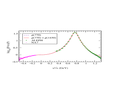
Figure 1: VFF fits for one and two resonances to the ALEPH data [6]. Also shown are the space-like data from NA7 [8].

$$\begin{array}[]{l}M_{\rho}^{\mathrm{pole}}\,=\,\left(764.1\pm 2.7\,{}^{+4.0}_{-2.5}\right)\>\mbox{MeV}\,,\\[10.0pt] \Gamma_{\rho}^{\mathrm{pole}}\,=\,\left(148.2\pm 1.9\,{}^{+1.7}_{-5.0}\right)\>\mbox{MeV}\,.\end{array}$$ (11)

We have also analyzed the influence of the chosen renormalization scale. The heavy resonance saturation of the $\chi$PT coupling constant $L_{9}^{r}(\mu)$ was studied through Eq. (10), together with the determination of ${M_{V}^{r}}(\mu)^{2}$, from fits performed at different values of $\mu$. The fit was repeated for a wide range of scales between 500 and 1200 MeV, obtaining the points shown in Fig. 2. The agreement with the predicted $\chi$PT running [2] is complete, i.e. the high-energy parameters run in the proper way to reproduce the low-energy dynamics. At $\mu_{0}=770$ MeV, we obtain $L_{9}^{r}(\mu_{0})=(7.04\pm 0.05\,{}^{+0.19}_{-0.27})\cdot 10^{-3}$.

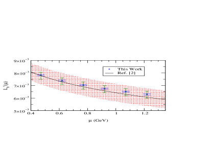
Figure 2: Variation of $L_{9}^{r}(\mu)$ with $\mu$, compared with the predicted $\chi$PT running [2]. We show statistical and statistical + systematic error bands.

6 Conclusions

It is important to incorporate the proper energy dependence of the observables when making accurate determinations of the resonance and chiral parameters. This becomes particularly relevant when one tries to obtain scale-independent properties as the pole mass and width, defined in the complex plane, from extrapolations of the data which sits in the real $q^{2}$–axis. Our analysis controls properly the momentum dependence, taking special care of analyticity and unitarity.

Working within the single-resonance approximation, we have obtained a good fit to the ALEPH data [6], in the range $2m_{\pi}^{2}<\sqrt{q^{2}}<1.2~{}\mbox{GeV}$. The fitted VFF is not sensitive to the chosen renormalization scale. However, performing fits at different values of $\mu$, we recover the proper running of the $\chi$PT coupling $L_{9}^{r}(\mu)$ from the $\mu$–dependent R$\chi$T parameters, showing how resonance saturation occurs at arbitrary scales.

In Ref. [1] it was also checked that the deviations of the fitted couplings from their large-$N_{C}$ predictions [4] are of the expected $1/N_{C}$ order, i.e. $F^{r}_{V}/F=\sqrt{2}+{\cal O}(1/N_{C})$ and $2\,G^{r}_{V}/F=\sqrt{2}+{\cal O}(1/N_{C})$. The numerical impact of the $\rho(1450)$ and of the exchange of heavy resonances in the $t$–channel was also tested. These effects are tiny for $\sqrt{s}\mathrel{\hbox to0.0pt{\lower 4.0pt\hbox{\hskip 1.0pt$\sim$}\hss}\raise 1.0pt\hbox{$<$}}1.2$ GeV but become relevant at higher energies.

References

- [1] J.J. Sanz-Cillero and A. Pich, Eur. Phys. J. C27 (2003) 587.
- [2] J. Gasser and H. Leutwyler, Nucl. Phys. B250 (1985) 465.
- [3] G. Ecker, J. Gasser, A. Pich and E. de Rafael, Nucl. Phys. B321 (1989) 311.
- [4] G. Ecker, J. Gasser, H. Leutwyler, A. Pich and E. de Rafael, Phys. Lett. B223 (1989) 425.
- [5] G. Ecker, Prog. Part. Nucl. Phys. 35 (1995) 1; A. Pich, Rep. Prog. Phys. 58 (1995) 563.
- [6] ALEPH Collaboration, Z. Phys. C76 (1997) 15.
- [7] CLEO Collaboration, Phys. Rev. D61 (2000) 112002; OPAL Collaboration, Eur. Phys. J. C7 (1999) 571; CMD-2 Collaboration, Phys. Lett. B527 (2002) 161.
- [8] NA7 Collaboration, Nucl. Phys. B277 (1986) 168.
- [9] G. ’t Hooft, Nucl. Phys. B72 (1974) 461, B75 (1974) 461; E. Witten, Nucl. Phys. B160 (1979) 57.
- [10] A. Pich, I. Rosell and J.J. Sanz-Cillero (in preparation).
- [11] A. Pich, in Phenomenology of Large– QCD, ed. R.F. Lebed, (World Scientific, Singapore, 2002) 239 [arXiv:hep-ph/0205030].
- [12] G.P. Lepage and S.J. Brodsky, Phys. Rev. D22 (1980) 2157.
- [13] F. Guerrero and A. Pich, Phys. Lett. B412 (1997) 382; A. Pich and J. Portolés, Phys. Rev. D63 (2001) 093005.
- [14] D. Gómez Dumm, A. Pich and J. Portolés, Phys. Rev. D62 (2000) 054014.
- [15] G.J. Gounaris and J.J. Sakurai, Phys. Rev. Let. 21 (1968) 244.