Confinement as Felt by Hadrons

Abstract

The critical behavior of non-order parameter fields is discussed. We show that relevant features of the deconfining phase transition can be determined by monitoring universal properties induced by the order parameter on the physical excitations. Some of the behaviors we uncover are already supported by lattice results.

1 Introduction

Properties of phase transitions are conveniently investigated using order parameters. However, the order parameter may not always be phenomenologically accessible. Besides, in nature most fields are non-order parameter fields. This lead to the question whether it is possible to extract relevant information about, or even identify, the onset of a phase transition using non-order parameter fields. We predict a universal behavior of a non order parameter field induced by the order parameter field near and at the phase transition. We also illustrate how to extract relevant features of the deconfining phase transition by monitoring the critical properties of the physical excitations [1, 2, 3, 4].

To derive the general properties of a singlet field we couple this to the order parameter [2]. In this way we can directly study the transfer of information, envisioned in [1], of the phase transition properties from the order parameter to the singlet field. The first studies, dealing with the information transfer from Polyakov loops to the hadronic states in pure Yang-Mills theory, are reviewed in [4].

Here we go beyond constant field approximation [2] and analyze two cases: time dependent order parameter fields and time independent ones [3]. Although time independent order parameter fields carry physical information about the phase transition, they do not propagate and cannot be canonically quantized. An example is the Polyakov loop, which is considered to be the order parameter of the pure Yang-Mills theory, and by construction is a function of space only. Time-dependent order parameter fields are generally associated with physical states. These can be composite, such as the chiral condensate, the order parameter related to chiral symmetry in QCD, or elementary, such as the Higgs field might be for the electroweak phase transition. The non-order parameter field, always time-dependent, is a singlet in particular under the symmetry group whose breaking is monitored by the order parameter. We assume the non-order parameter field to have a large mass with respect to all the other scales in play, and hence, an associated small correlation length near the phase transition. A generic singlet field in the Yang-Mills theory is the glueball, which is also a physical state of the theory.

Using general field theoretical arguments we demonstrate that the screening mass associated with the spatial two-point function of the singlet field is strongly affected by the nearby phase transition for both time-dependent and time-independent order parameters. More specifically, the screening mass has a drop near the phase transition. This is due to the three dimensional nature of the screening mass, which makes it particularly sensitive to infrared physics and it explains the transfer of information between the order parameter and the singlet field. We also study the effects of a phase transition on the pole mass of the singlet field in the four dimensional theory, and find that only the spatial correlation lengths feel the presence of a nearby phase transition.

Our main conclusion in both cases is that the information about the phase transition, encoded in the behavior of the order parameter field is transferred to, and obtainable from the singlet field(s) present in the theory.

2 General Theory

We consider a temperature driven phase transition and work in a regime close to the phase transition. In order for our results to be as universal as possible, we use a general renormalizable Lagrangian containing a field neutral under the global symmetries, and the order parameter field, as well as their interactions. The protagonists of our theory are two real fields, $h$ and $\chi$. The field $h$ is a scalar singlet, while $\chi$ transforms according to $\chi\rightarrow z\,\chi$ with $z\in Z_{N}$. While the generalization to $Z_{N}$ is straightforward, we consider explicitly the case of $Z_{2}$, which is suitable for understanding the deconfining phase transition of 2 color Yang-Mills. This has been heavily studied via lattice simulations [5, 6]. The potential is

$$V(h,\chi) = \frac{m^{2}}{2}h^{2}+\frac{m^{2}_{0\chi}}{2}\,\chi^{2}+\frac{\lambda}{4!}\chi^{4}+g_{0}h$$ (1)

$$+ \frac{g_{1}}{2}\,h\chi^{2}+\frac{g_{2}}{4}\,h^{2}\chi^{2}+\frac{g_{3}}{3!}h^{3}+\frac{g_{4}}{4!}h^{4}\,.$$

The coefficients are real. Stability requires $\lambda\geq 0$ and $g_{4}\geq 0$. Assuming $g_{1}>0$ and $g_{0}<0$ assures that the extremum of the potential is a minimum. This renormalizable potential can be considered, for example, as a truncation of the one presented in [1, 4], and can be used to determine some of the space-time independent properties of the vacuum.

We conduct our analysis using the following assumptions : i) The $\chi$ field is light close to the transition, is massless at the transition point, hence it dominates the dynamics. ii) The $h$ field is heavy, and thus we can neglect its quantum and Boltzman suppressed thermal loop corrections.

The temperature dependence of the minimum of the linearized potential is qualitatively sketched in Figure 1 of [4], and it is discussed in [3] in more detail.

In the following we discuss the fluctuations of $h$ around its vacuum expectation value and evaluate the spatial correlators.

3 3D Order Parameter

We have chosen $\chi=\chi({\bf{x}})$ and decomposed the four dimensional $h$ field into its Matsubara modes. After integrating over time the action reduces to an effective three dimensional one. The kinetic term for $h$ and its self-interaction terms receive contributions from all Matsubara modes. However, only the zero mode contributes to the $h\chi^{2}$–interaction, which drives the dynamics of the $h$ field close to the phase transition [2], as the $\chi$ field becomes light with respect to $h$. Therefore, we confine our discussion to the theory which features the fields $\chi$ and $h_{0}$. For simplicity, we denote $h_{0}$ by $h$ which is taken to be directly the fluctuation field around its tree level vacuum expectation value. The three dimensional Lagrangian reads:

$$-{\cal L}_{3} = \frac{1}{2}\nabla h\nabla h+\frac{1}{2}\nabla\chi\nabla\chi+\frac{1}{2}m^{2}h^{2}+\frac{1}{2}m^{2}_{\chi}\chi^{2}\$$ (2)

$$+ T\frac{\lambda}{4!}(\chi^{2})^{2}+\sqrt{T}\frac{g_{1}}{2}\,h\chi^{2}+T\frac{g_{2}}{4}\,h^{2}\chi^{2}$$

$$+ \sqrt{T}\frac{g_{3}}{3!}h^{3}+T\frac{g_{4}}{4!}h^{4}\,,$$

where the coupling constants have the same mass dimension as in the corresponding four dimensional theory.

The full expression of the $h$ two-point function at one-loop level is given by the following set of diagrams:

(3)

Double lines indicate $\chi$ fields and single lines stand for the $h$ field. We regularize all the ultraviolet divergent contributions. The second diagram is infrared divergent for $T\rightarrow T_{c}$ and gives the dominant one loop contribution to the screening mass of $h$. This is true both in the symmetric and symmetry broken phases. In the limit of zero external momentum

$$m^{2}(T)=m^{2}-T\,\frac{g^{2}_{1}}{16\pi m_{\chi}}+{\cal{O}}(m_{\chi})\,.$$ (4)

Equation (4) illustrates how the nearby phase transition is directly felt by the non-order parameter field. Furthermore, it gives the general prediction that the screening mass of the singlet field must decrease close to the phase transition. If we stop the analysis here, at one-loop level, we predict the following critical behavior for $\Delta m^{2}=m^{2}(T)-m^{2}$, where $m$ is the mass at a temperature close to the critical point:

$$\Delta m^{2}(T) = -\frac{g_{1}^{2}\,T}{16\pi\,m_{\chi}}\sim t^{-\frac{\nu}{2}},\quad T<T_{\rm{c}}$$ (5)

$$\Delta m^{2}(T) = -\frac{g_{1}^{2}\,T}{16\pi\,M_{\chi}}\sim t^{-\frac{\nu}{2}},\quad T>T_{\rm{c}}$$ (6)

where $M_{\chi}=\sqrt{2}|m_{\chi}|\propto|T-T_{c}|^{\nu/2}$. This one-loop result breaks down at the transition point, due to the infrared singularity. But since $h$ is not the order parameter field, its correlation length ($1/m$) is not expected to diverge at the transition point.

We now investigate the behavior of the $h$ screening mass near the phase transition by going beyond the one-loop approximation.

3.1 Healing the IR behavior

When analyzing contributions beyond one-loop order to the $h$ two-point function, the number of diagrams, and distinct topologies one needs to consider proliferates. We select a subclass of diagrams, that heal the infrared divergences, while capturing the essential physical properties of the problem at hand. A finite result for the two-point function, both in the broken and unbroken phases will emerge, while the expression for the mass of $h$ turns out to be continuous across $T_{c}$.

In the unbroken phase it is known, that for a generic $O(N)$ theory in the large $N$ limit the following chain of bubble diagrams represents the leading contribution,

These diagrams constitute a geometrical series and their resummation is exact [7]. We choose the same set of diagrams in the unbroken phase. We note that a large $N$ approximation might not be the best choice for investigating the details of the phase transition, however we show that it well reproduces the behavior of the screening mass of hadronic degrees of freedom near the deconfinement phase transition as given by lattice simulations. After summation the following expression for $m$ follows:

$$m^{2}(T)=m^{2}-T\,\frac{g_{1}^{2}}{16\pi\,m_{\chi}+\lambda\,T}\,,$$ (7)

which is finite at $T_{c}~{}$, where it yields:

$$m^{2}(T_{c})=m^{2}-\frac{g_{1}^{2}}{\lambda}\,.$$ (8)

This is the main result of [2], predicting that close to the phase transition the singlet state must have a decreasing mass parameter, associated with spatial correlations. More specifically, the drop at the phase transition point is given by the ratio of the square of the coupling constant governing the interaction of the singlet state with the order parameter ($g_{1}$) to the order parameter field self-interaction coupling constant $\lambda$. In this way, via the drop of the singlet field at the phase transition, one can derive a great deal of information about the phase transition, and about the order parameter itself.

The analysis is much more complicated in the broken phase. Here $\chi$ develops an average value, $v$, which induces one also for $h$ [3]. So on general grounds, the fields $\chi$ and $h$ mix in this phase. The mixing angle is proportional to $g_{1}\,v/m^{2}~{}$, and therefore, this mixing can be neglected within the present approximations. Like for the symmetric phase, we consider only the effects due to the $\chi$ loops for the $h$ propagator. Due to symmetry breaking we now need to include also the trilinear $\chi$ coupling

$$-\frac{\lambda}{3!}\,v\,\chi^{3}\,,$$ (9)

which is expected to affect the analysis. Curing the infrared divergence is thus now more involved due to symmetry breaking. In the case of the large $N$ limit of $O(N)$ symmetry, one can show, that diagrams with trilinear vertices are again suppressed relative to the simple bubble diagrams. But now we go beyond the large $N$ limit by computing a new set of diagrams, which can be evaluated exactly, and thus capture relevant corrections due to symmetry breaking, neglected in the large $N$ limit. The new chain of diagrams we compute has terms of the form:

(10)

This class of diagrams has knowledge about the onset of symmetry breaking via the presence of the trilinear vertices, and, in that respect, is the simplest extension of the chain of simple bubble diagrams. Another amusing property of (10) is, that the sum can be performed exactly, yielding again an infrared finite result:

$$m^{2}(T)=m^{2}-g_{1}^{2}T\frac{24\pi M_{\chi}+\lambda T}{\lambda^{2}T^{2}+24\pi\lambda TM_{\chi}+384\pi^{2}M_{\chi}^{2}}\,.$$ (11)

We see that $m(T_{c})$ from the broken side of the transition equals exactly the one from the unbroken side of the transition, even when departing from the large $N$ limit. The mass squared of $h$ is a continuous function through the phase transition, and the associated correlation length remains finite. This result does not hold order by order in the loop expansion, but only when the infinite sum of the diagrams is performed.

In order to disentangle relevant properties of the phase transition, we construct slope parameters for the singlet field:

$${\cal D}^{\pm} \equiv \lim_{T\rightarrow T_{\rm{c}}^{\pm}}\frac{1}{\Delta m^{2}(T)}\frac{d\,m^{2}(T)}{dT}\,,$$ (12)

with $\Delta m^{2}(T_{c})=g_{1}^{2}/\lambda~{}$. The functional form of $\cal{D}^{+}$ and $\cal{D}^{-}$ is the same, provided that the same class of diagrams is resummed on both sides of the transition. In such case:

$${\cal D}^{-}=\frac{16\,\pi}{\lambda\,T_{c}}\lim_{T\rightarrow T_{c}^{-}}\frac{d\,m_{\chi}}{dT}$$ (13)

in the symmetric phase, and ${\cal D}^{+}$ in the broken phase is obtained by replacing $m_{\chi}$ with $M_{\chi}=\sqrt{2}|m_{\chi}|$. While the mass of $h$ remains finite at $T_{c}$, its slope encodes the critical behavior of the theory. For example, if $m^{2}_{\chi}$ vanishes as $(T_{c}-T)^{\nu}$ close to the phase transition (with the correlation length $\xi\propto|T-T_{c}|^{-{\nu}/{2}}$), then ${\cal D}^{\pm}$ scale with exponent $(\nu/2-1)$. A difference in the functional form of the slopes may emerge, when on the two sides of the transition different class of diagrams are resummed. Using the wider class of diagrams in the broken phase considered above while retaining just the simple bubble sum in the unbroken we determine:

$${\cal D}^{+}\simeq-3\,\frac{16\pi}{\lambda T_{c}}{|m_{\chi}|}{\cal D}^{-}\,.$$ (14)

This is due to the onset of spontaneous symmetry breaking, i.e. in the broken phase the class of resummed diagrams contains trilinear type of interactions. We identify thus a less singular behavior with respect to the simple sum of bubbles. More specifically, the scaling exponent for ${\cal D}^{+}$ is now $(\nu-1)$. While the explicit relations between the scaling exponents and the slopes are only valid within the given summation scheme, these quantities are, nevertheless, a measure of the critical behavior near the phase transition. Only experimental results will be able to select which class best describes the data.

In figure 1 we schematically present the behavior of the $h$ screening mass as a function of temperature, in units of the critical temperature, for $m^{2}_{\chi}\propto(T_{c}-T)~{}$.

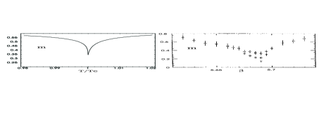
Figure 1: Left panel: Screening mass of the singlet field close to the phase transition as function of the temperature. Right panel: Lattice data; figure from [8].

The left panel illustrates the rapid decrease of the singlet field screening mass in the critical region. The right panel is the lattice data of [8] obtained for the glueball screening mass in the three color Yang-Mills theory. The resemblance between our results and the lattice results is intriguing, but more lattice data is needed in order to distinguish between the above possibilities, and quantitatively determine the size of the drop.

4 4D Order Parameter

Here we present the effects of the four dimensional $\chi=\chi({\bf{x}},t)$ order parameter field on the properties of a singlet $h=h({\bf{x}},t)$ field. The order parameter field is now a physical field, and as such, it can propagate in time, and can be canonically quantized. The four-dimensional Lagrangian of the renormalizable theory we use to define our Feynman rules is:

$${\cal L}_{4} = \frac{1}{2}\partial_{\mu}h\partial^{\mu}h+\frac{1}{2}{\partial_{\mu}}\chi{\partial^{\mu}}\chi-\frac{m^{2}}{2}h^{2}-\frac{m^{2}_{\chi}}{2}\,\chi^{2}$$ (15)

$$- \frac{\lambda}{4!}\chi^{4}-\frac{g_{1}}{2}\,h\chi^{2}-\frac{g_{2}}{4}\,h^{2}\chi^{2}-\frac{g_{3}}{3!}h^{3}-\frac{g_{4}}{4!}h^{4}\,.$$

All coupling constants are real and $\lambda,g_{4}\geq 0$. The relevant and marginal couplings, in terms of dimensionless ones, are $g_{1}=\hat{g}_{1}m~{}$, $g_{3}=\hat{g}_{3}m~{}$ and $g_{2}=\hat{g}_{2}~{}$. The $\chi$ field is subject to $Z_{2}$ symmetry. In four dimensions a Bose-Einstein distribution emerges for $\chi$, and thus thermal fluctuations become important. These have the tendency to restore symmetry, destroying the possibility for the formation and existence of any physical condensate at high temperatures.

The diagrams contributing to the $h$ two-point function at one-loop order are shown in (3). Even though these are the same as in the three dimensional theory, here they are computed taking into account the time dependence of $\chi$. We can show, that finite temperature corrections from all diagrams that involve an $h$ loop are Boltzman suppressed. Thus the relevant diagrams for the singlet $h$ field are those on the first line in (3). Unlike the three dimensional case where ultraviolet divergent tadpoles have been removed by renormalization, in the four dimensions these diagrams also provide temperature contributions. The diagrams are evaluated using standard techniques of the imaginary time formalism [9]. The tadpoles are real and provide temperature dependence to the $h$ mass, not present in the three dimensional theory. The eye diagram has a real and an imaginary part contributing to the two-point function $\left[E^{2}-m^{2}-\Pi(E)\right]^{-1}~{}$. Here $m$ is the tree level mass of $h$ and at one-loop order $\Pi=\Pi_{tadpole}+\Pi_{eye}~{}$. For zero external momentum

$$\Pi_{eye}(E)=-\frac{g_{1}^{2}}{2}\int\frac{d^{3}k}{(2\pi)^{3}}\frac{1}{\omega}\frac{1}{E^{2}-4\omega^{2}}(1+2f(\omega))\,,$$ (16)

with $\omega=\sqrt{{\bf{k}}^{2}+{m_{\chi}}^{2}}~{}$, and $f$ Bose distribution function. The real part is given by the principal value of (16), and represents a shift in the mass squared of the $h$. For $h$ at rest, the real part by its definition determines the pole mass $M$, i.e. the pole of the full two-point function

$${M}^{2}-m^{2}-\Pi_{tadpole}-\mbox{Re}~{}\Pi_{eye}(E=M)=0\,.$$ (17)

Self-consistent solution of the above equation shows that the large tree level mass dominates, and loop corrections are negligibly small in the temperature range of interest, near the phase transition. Thus $M\simeq m$ acts as an infrared cutoff, guaranteeing the absence of infrared divergence in the pole mass. All the one-loop contributions to the pole mass sum to

$$M^{2}\simeq m^{2}\left[1+\left(\hat{g}_{2}-\hat{g}_{1}\hat{g}_{3}-2\hat{g}^{2}_{1}\right)\,\frac{T^{2}}{24\,m^{2}}\right]\,.$$ (18)

It is important to distinguish between the pole mass and the screening mass. The screening mass, $m_{s}$, is defined by the location of the pole in the static propagator for complex momentum $p=im_{s}$,

$$p^{2}+\Pi(E=0,p)=0\,.$$ (19)

In the small momentum limit this leads to the following definition

$$m_{s}^{2}=m^{2}+\lim_{p\rightarrow 0}\Pi(E=0,p)\,.$$ (20)

In three dimensions the pole and screening masses are the same, since the static propagator is the full propagator. We have shown, that when looking at the pole mass the IR problem of the eye diagram is regulated by the heavy $h$ mass. When analyzing the screening mass, however, the one-loop IR divergence present in the three dimensional case is recovered. This can be seen by setting $E=0$ in expression (16) corresponds to reducing the 4D theory to a 3D one. To display the relevant infrared contribution we take the high temperature expansion which yields:

$$2\left(\frac{g_{1}}{2}\right)^{2}\frac{T}{4\pi^{2}}\int_{0}^{\infty}dp\frac{p^{2}}{(p^{2}+m_{\chi}^{2})^{2}}=g_{1}^{2}\frac{T}{32\pi m_{\chi}}\,.$$ (21)

Thus, for the static limit the phase transition region is dominated by the same type of infrared divergence we encountered in the time-independent order parameter field case. Note, however, that the numerical constant in eq. (21) differs from that in the second term of eq. (4). The reason for this is that the reduction was done only for the modes of $h$, and thus in eq. (21), contrary to (4), all Matsubara modes of $\chi$ contribute. By combining all the tadpole and eye diagrams we find for the screening mass at one-loop order

$$m_{s}^{2}\simeq m^{2}\left[1-\frac{\hat{g}_{1}^{2}}{32\pi}\frac{T}{m_{\chi}}-\left({\hat{g}_{1}\hat{g}_{3}}-{\hat{g}_{2}}\right)\frac{T^{2}}{24\,m^{2}}\right]\,,$$ (22)

showing clearly the eye contribution as the infrared dominant one. Note also, that above we have tree level coefficients, and a complete investigation would require renormalization group analysis.

5 Deconfinement and Conclusions

When analyzing many physical situations, it is common practice to isolate the order parameter field, and more generally, the light degrees of freedom, since these are expected to be the relevant states at low energies. While this procedure certainly is reasonable, in nature most of the physical fields are neither order parameter fields, nor light at all. In order to extract information from these heavy states, we needed first to determine new and universal features associated with them. We have used a general strategy proposed first in [1, 2], according to which we couple the light degrees/order parameter fields to the heavy fields in the most general way, and then truncate the theory by retaining all the relevant and marginal operators in the Lagrangian. In doing so, the theory is fully renormalizable while capturing the relevant contributions. The operator set is further constrained by imposing the relevant symmetries of the problem at hand. In order for our procedure to work, we also assume, that the other physical states of the theory have masses larger than our non-order parameter field. In this way we can, formally, integrate these states out, and their effects are absorbed in the modified couplings of our effective Lagrangian.

For both the time independent and time dependent order parameter field we have shown [3], that the spatial correlators of the non-order parameter field are infrared dominated, and hence can be used to determine the properties of the phase transition. We have determined the general behavior of the screening mass of a generic singlet field, and have shown how to extract all the relevant information from such a quantity. We have further demonstrated, that the pole mass of any non-order parameter physical field is not infrared dominated.

Our results can be immediately applied to any generic phase transition. We have used as relevant example, for the time independent order parameter field case, the deconfining transition of Yang-Mills theories. In [1] a model containing glueball $H$ and Polyakov loop $\ell(\vec{x})$ was proposed, and is supported by other investigations [11]. The present results can be understood as the higher loop corrections to the glueball model in [1] and can be immediately applied to the two color Yang-Mills phase transition, once we associate $H$ with $h$, and $\ell$ with $\chi$. For example one can take the following relation between $H$ and the glueball field $h$:

$$H=\langle H\rangle\left(1+\frac{h}{\sqrt{c}\langle H\rangle^{1/4}}\right)\ .$$ (23)

Here $\langle H\rangle=\Lambda^{4}/e$ is the vacuum expectation value of the glueball field below the critical temperature and $c$ is a positive dimensionless constant fixed by the mass of the glueball. For the $\ell$ field we have $\chi=\sqrt{\kappa}\ell$ with $\kappa$ a mass dimension two constant, which at high temperature is proportional to $T^{2}$. Specifically, our renormalizable theory is a truncated (up to fourth order in the fields) version of the full glueball theory.

We confronted already our theoretical results with lattice computations of the glueball screening mass behavior close to the phase transition studied in [8] for three colors. Our analysis not only is in agreement with the numerical analysis, but also allows us to provide a better understanding of the physics in play. Further lattice simulations are able to determine the coupling strength of any glueball state to the Polyakov loop by following the temperature dependence of screening masses of such states.

Our analysis suggests, that monitoring a number of spatial correlators, or more specifically their derivatives, is an efficient and sufficient way to experimentally uncover the chiral/deconfining phase transition and its features.

The findings here provide a general computational strategy useful to deduce new quantitative information about any phase transition. Using this strategy we were also able to explain how deconfinement is linked to chiral symmetry restoration [12].

References

- [1] F. Sannino, Phys. Rev. D 66, 034013 (2002) [arXiv:hep-ph/0204174].
- [2] A. Mocsy, F. Sannino and K. Tuominen, Phys. Rev. Lett. 91, 092004 (2003) [arXiv:hep-ph/0301229].
- [3] A. Mocsy, F. Sannino and K. Tuominen, Induced universal properties and deconfinement, arXiv:hep-ph/0306069.
- [4] A. Mocsy, F. Sannino and K. Tuominen, Connecting Ployakov Loops to Hadrons, in these proceedings. arXiv:hep-ph/0310078.
- [5] P.H. Damgaard, Phys. Lett. B194 (1987) 107; J. Kiskis, Phys. Rev. D41 (1990) 3204; J. Fingberg et al., Phys. Lett. B248 (1990) 347; J. Christensen and P.H. Damgaard, Nucl. Phys. B348 (1991) 226; P.H. Damgaard and M. Hasenbush, Phys. Lett. B331 (1994) 400: J. Kiskis and P. Vranas, Phys. Rev. D49 (1994) 528.
- [6] S. Hands, Nucl. Phys. Proc. Suppl. 106, 142 (2002) [arXiv:hep-lat/0109034].
- [7] S. R. Coleman, R. Jackiw and H. D. Politzer, Phys. Rev. D 10, 2491 (1974).
- [8] For early studies on the relation between glueballs and Polyakov loops see: P. Bacilieri et al. [Ape Collaboration], Phys. Lett. B 220, 607 (1989).
- [9] J. I. Kapusta, Finite-temperature Field Theory, Cambridge University Press, Cambridge (1989).
- [10] N. O. Agasian, JETP Lett. 57, 208 (1993) [Pisma Zh. Eksp. Teor. Fiz. 57, 200 (1993)].
- [11] P. N. Meisinger and M. C. Ogilvie, Phys. Rev. D 66, 105006 (2002) [arXiv:hep-ph/0206181].
- [12] A. Mocsy, F. Sannino and K. Tuominen, Confinement versus chiral symmetry, arXiv:hep-ph/0308135.