Structure of the nucleon in chiral perturbation theory

Abstract

We discuss a renormalization scheme for relativistic baryon chiral perturbation theory which provides a simple and consistent power counting for renormalized diagrams. The method involves finite subtractions of dimensionally regularized diagrams beyond the standard modified minimal subtraction scheme of chiral perturbation theory to remove contributions violating the power counting. This is achieved by a suitable renormalization of the parameters of the most general effective Lagrangian. As applications we discuss the mass of the nucleon, the $\sigma$ term, and the scalar and electromagnetic form factors.

1 Introduction

Starting from Weinberg’s pioneering work Weinberg:1979kz , the application of effective field theory (EFT) to strong interaction processes has become one of the most important theoretical tools in the low-energy regime. The basic idea consists of writing down the most general possible Lagrangian, including all terms consistent with assumed symmetry principles, and then calculating matrix elements with this Lagrangian within some perturbative scheme Weinberg:1979kz . A successful application of this program thus requires two main ingredients:

1. a knowledge of the most general effective Lagrangian;

2. an expansion scheme for observables in terms of a consistent power counting method.

The structure of the most general Lagrangian for both mesonic and baryonic chiral perturbation theory (ChPT) has been investigated for almost two decades. The number of terms in the momentum and quark-mass expansion is given by

$$\underbrace{2}_{\mbox{${\cal O}(q^{2})$}}+\underbrace{10+2}_{\mbox{${\cal O}(q^{4})$}}+\underbrace{90+4+23}_{\mbox{${\cal O}(q^{6})$}}+\cdots$$

for mesonic ChPT [SU(3)$\times$SU(3)] GL ; p6 and

$$\underbrace{2}_{\mbox{${\cal O}(q)$}}+\underbrace{7}_{\mbox{${\cal O}(q^{2})$}}+\underbrace{23}_{\mbox{${\cal O}(q^{3})$}}+\underbrace{118}_{\mbox{${\cal O}(q^{4})$}}+\cdots$$

for baryonic ChPT [SU(2)$\times$SU(2)$\times$U(1)] Gasser:1988rb ; Krause:xc ; Ecker:1995rk ; Meissner:1998rw ; Fettes:2000gb . Moreover, the mesonic sector contains at ${\cal O}(q^{4})$ the Wess-Zumino-Witten action Wess:yu ; Witten:tw taking care of chiral anomalies.

Once the most general effective Lagrangian is known, one needs an expansion scheme in order to perform perturbative calculations of physical observables. In this context one faces the standard difficulties of encountering ultraviolet divergences when calculating loop diagrams. However, since one is working with the most general Lagrangian containing all terms allowed by the symmetries, these infinities can, as part of the renormalization program, be absorbed by a suitable adjustment of the parameters of the Lagrangian Weinberg:1979kz ; Weinberg:mt . Applying dimensional regularization in combination with the modified minimal subtraction scheme of ChPT, in the mesonic sector a straightforward correspondence between the loop expansion and the chiral expansion in terms of momenta and quark masses at a fixed ratio was set up by Gasser and Leutwyler GL . The situation in the one-nucleon sector turned out to be more complicated Gasser:1988rb , since the correspondence between the loop expansion and the chiral expansion seemed to be lost. One of the findings of Ref. Gasser:1988rb was that higher-loop diagrams can contribute to terms as low as ${\cal O}(q^{2})$. A solution to this problem was obtained in the framework of the heavy-baryon formulation of ChPT Jenkins:1990jv ; Bernard:1992qa resulting in a power counting analogous to the mesonic sector (for a recent review of ChPT see, e.g., Ref. Scherer:2002tk ).

Here, we will review some recent efforts to devise a new renormalization scheme leading to a simple and consistent power counting for the renormalized diagrams of a manifestly covariant approach. The basic idea consists in performing additional subtractions of dimensionally regularized diagrams beyond the modified minimal subtraction scheme employed in Ref. Gasser:1988rb . As applications we will discuss the mass of the nucleon as well as the scalar and electromagnetic form factors and compare the method with the approach of Becher and Leutwyler Becher:1999he .

2 Dimensional regularization

Figure 1: Generic one-loop diagram. The black box denotes some unspecified vertex structure which is irrelevant for the discussion.

For the regularization of loop diagrams we will make use of dimensional regularization dimreg , because it preserves algebraic relations between Green functions (Ward identities). We will illustrate the method by considering the following simple example,

$$I(M^{2})=\int\frac{d^{4}k}{(2\pi)^{4}}\frac{i}{k^{2}-M^{2}+i0^{+}},\quad k^{2}=k_{0}^{2}-\vec{k}\,^{2},$$ (1)

which shows up in the generic diagram of Fig. 1. Naively counting the powers of the momenta, the integral is said to diverge quadratically. In order to regularize Eq. (1), we define the integral for $n$ dimensions ($n$ integer) as

$$I_{n}(M^{2},\mu^{2})=\mu^{4-n}\int\frac{d^{n}k}{(2\pi)^{n}}\frac{i}{k^{2}-M^{2}+i0^{+}},$$

where the scale $\mu$ (’t Hooft parameter) has been introduced so that the integral has the same dimension for arbitrary $n$. After a Wick rotation and angular integration, the analytic continuation for complex $n$ reads (see Appendix B of Ref. Scherer:2002tk for details)

$$I(M^{2},\mu^{2},n) = \frac{M^{2}}{(4\pi)^{2}}\left(\frac{4\pi\mu^{2}}{M^{2}}\right)^{2-\frac{n}{2}}\Gamma\left(1-\frac{n}{2}\right)$$ (2)

$$= \frac{M^{2}}{16\pi^{2}}\left[R+\ln\left(\frac{M^{2}}{\mu^{2}}\right)\right]+O(n-4),$$

where

$$R=\frac{2}{n-4}-[\mbox{ln}(4\pi)+\Gamma^{\prime}(1)]-1.$$ (3)

The idea of renormalization consists of adjusting the parameters of the counterterms of the most general effective Lagrangian so that they cancel the divergences of (multi-) loop diagrams. In doing so, one still has the freedom of choosing a suitable renormalization condition. For example, in the minimal subtraction scheme (MS) one would fix the parameters of the counterterm Lagrangian such that they would precisely absorb the contributions proportional to $2/(n-4)$ in Eq. (3), while the modified minimal subtraction scheme ($\overline{\rm MS}$) would, in addition, cancel the term in square brackets. Finally, in the modified minimal subtraction scheme of ChPT ($\widetilde{\rm MS}$) employed in Ref. GL , the seven (bare) coefficients $l_{i}$ of the ${\cal O}(q^{4})$ Lagrangian are expressed in terms of renormalized coefficients $l_{i}^{r}$ as

$$l_{i}=l_{i}^{r}+\gamma_{i}\frac{R}{32\pi^{2}},$$ (4)

where the $\gamma_{i}$ are fixed numbers.

3 Mesonic chiral perturbation theory

The starting point of mesonic chiral perturbation theory is a chiral $\mbox{SU(2)}_{L}\times\mbox{SU(2)}_{R}$ symmetry of the two-flavor QCD Lagrangian in the limit of massless $u$ and $d$ quarks. It is assumed that this symmetry is spontaneously broken down to its isospin subgroup SU(2)_V, i.e., the ground state has a lower symmetry than the Lagrangian. From Goldstone’s theorem one expects $6-3=3$ massless Goldstone bosons which interact “weakly” at low energies, and which are identified with the pions of the “real” world. The explicit chiral symmetry breaking through the quark masses is included as a perturbation. According to the program of EFT the symmetries of QCD are mapped onto the most general effective Lagrangian for the interaction of the Goldstone bosons (pions). The Lagrangian is organized in a derivative and quark-mass expansion Weinberg:1979kz ; GL ; p6

$${\cal L}_{\pi}={\cal L}_{2}+{\cal L}_{4}+{\cal L}_{6}+\cdots,$$ (5)

where—in the absence of external fields—the lowest-order Lagrangian is given by GL

$${\cal L}_{2}=\frac{F^{2}}{4}\mbox{Tr}\left(\partial_{\mu}U\partial^{\mu}U^{\dagger}\right)+\frac{F^{2}M^{2}}{4}\mbox{Tr}(U^{\dagger}+U),$$ (6)

with

$$U=\exp\left(i\frac{\vec{\tau}\cdot\vec{\pi}}{F}\right)$$

a unimodular unitary $(2\times 2)$ matrix containing the Goldstone boson fields. In Eq. (6), $F$ denotes the pion-decay constant in the chiral limit: $F_{\pi}=F[1+{\cal O}(\hat{m})]=92.4$ MeV. Here, we work in the isospin-symmetric limit $m_{u}=m_{d}=\hat{m}$, and the lowest-order expression for the squared pion mass is $M^{2}=2B\hat{m}$, where $B$ is related to the quark condensate $\langle\bar{q}q\rangle_{0}$ in the chiral limit GL .

Using Weinberg’s power counting scheme Weinberg:1979kz one may analyze the behavior of a given diagram calculated in the framework of Eq. (5) under a linear rescaling of all external momenta, $p_{i}\mapsto tp_{i}$, and a quadratic rescaling of the light quark masses, $m_{q}\mapsto t^{2}m_{q}$, which, in terms of the Goldstone boson masses, corresponds to $M^{2}\mapsto t^{2}M^{2}$. The chiral dimension $D$ of a given diagram with amplitude ${\cal M}(p_{i},m_{q})$ is defined by

$${\cal M}(tp_{i},t^{2}m_{q})=t^{D}{\cal M}(p_{i},m_{q}),$$ (7)

where, in $n$ dimensions,

$$D = nN_{L}-2I_{\pi}+\sum_{k=1}^{\infty}2kN_{2k}^{\pi}$$ (8)

$$= 2+(n-2)N_{L}+\sum_{k=1}^{\infty}2(k-1)N_{2k}^{\pi}$$

$$\geq \mbox{2 in 4 dimensions}.$$

Here, $N_{L}$ is the number of independent loop momenta, $I_{\pi}$ the number of internal pion lines, and $N_{2k}^{\pi}$ the number of vertices originating from ${\cal L}_{2k}$. Clearly, for small enough momenta and masses diagrams with small $D$, such as $D=2$ or $D=4$, should dominate. Of course, the rescaling of Eq. (7) must be viewed as a mathematical tool. While external three-momenta can, to a certain extent, be made arbitrarily small, the rescaling of the quark masses is a theoretical instrument only. Note that, for $n=4$, loop diagrams are always suppressed due to the term $2N_{L}$ in Eq. (3). In other words, we have a perturbative scheme in terms of external momenta and masses which are small compared to some scale [here $1/(4\pi F)$].

Figure 2: One-loop contribution to the pion self-energy. The number 2 in the interaction blob refers to ${\cal L}_{2}$.

As an example, let us consider the contribution of Fig. 2 to the pion self-energy. According to Eq. (8) we expect, in 4 dimensions, the chiral power

$$D=4\cdot 1-2\cdot 1+2\cdot 1=4.$$

Without going into the details, the explicit result of the one-loop contribution is given by (see, e.g., Ref. Scherer:2002tk )

$$\Sigma_{\rm loop}(p^{2})=\frac{4p^{2}-M^{2}}{6F^{2}}I(M^{2},\mu^{2},n)={\cal O}(q^{4}),$$

where the integral is given in Eq. (2) and is infinite as $n\to 4$. Note that both factors—the fraction and the integral—each count as ${\cal O}(q^{2})$ resulting in ${\cal O}(q^{4})$ for the total expression as anticipated.

For a long time it was believed that performing loop calculations using the Lagrangian of Eq. (6) would make no sense, because it is not renormalizable (in the traditional sense). However, as emphasized by Weinberg Weinberg:1979kz ; Weinberg:mt , the cancellation of ultraviolet divergences does not really depend on renormalizability; as long as one includes every one of the infinite number of interactions allowed by symmetries, the so-called non-renormalizable theories are actually just as renormalizable as renormalizable theories Weinberg:mt . The conclusion is that a suitable adjustment of the parameters of ${\cal L}_{4}$ [see Eq. (4)] leads to a cancellation of the one-loop infinities.

4 Baryonic chiral perturbation theory and renormalization

The extension to processes involving one external nucleon line was developed by Gasser, Sainio, and Švarc Gasser:1988rb . In addition to Eq. (5) one needs the most general effective Lagrangian of the interaction of Goldstone bosons with nucleons:

$${\cal L}_{\pi N}={\cal L}_{\pi N}^{(1)}+{\cal L}_{\pi N}^{(2)}+\cdots.$$

The lowest-order Lagrangian, expressed in terms of bare fields and parameters denoted by subscripts 0, reads

$${\cal L}_{\pi N}^{(1)}=\bar{\Psi}_{0}\left(i\gamma_{\mu}\partial^{\mu}-m_{0}-\frac{1}{2}\frac{{\stackrel{{\scriptstyle\circ}}{{g_{A}}}}_{0}}{F_{0}}\gamma_{\mu}\gamma_{5}\tau^{a}\partial^{\mu}\pi^{a}_{0}\right)\Psi_{0}+\cdots,$$ (10)

where $\Psi_{0}$ denotes the (bare) nucleon field with two four-component Dirac fields describing the proton and the neutron, respectively. After renormalization, $m$ and $\stackrel{{\scriptstyle\circ}}{{g_{A}}}$ refer to the chiral limit of the physical nucleon mass and the axial-vector coupling constant, respectively. While the mesonic Lagrangian of Eq. (5) contains only even powers, the baryonic Lagrangian involves both even and odd powers due to the additional spin degree of freedom.

Our goal is to propose a renormalization procedure generating a power counting for tree-level and loop diagrams of the (relativistic) EFT which is analogous to that given in Ref. Weinberg:1991um (for nonrelativistic nucleons). Choosing a suitable renormalization condition will allow us to apply the following power counting: a loop integration in $n$ dimensions counts as $q^{n}$, pion and fermion propagators count as $q^{-2}$ and $q^{-1}$, respectively, vertices derived from ${\cal L}_{2k}$ and ${\cal L}_{\pi N}^{(k)}$ count as $q^{2k}$ and $q^{k}$, respectively. Here, $q$ generically denotes a small expansion parameter such as, e.g., the pion mass. In total this yields for the power $D$ of a diagram in the one-nucleon sector the standard formula Weinberg:1991um ; Ecker:1995gg

$$D = nN_{L}-2I_{\pi}-I_{N}+\sum_{k=1}^{\infty}2kN^{\pi}_{2k}+\sum_{k=1}^{\infty}kN_{k}^{N}$$

$$= 1+(n-2)N_{L}+\sum_{k=1}^{\infty}2(k-1)N^{\pi}_{2k}+\sum_{k=1}^{\infty}(k-1)N_{k}^{N}$$

$$\geq \mbox{1 in 4 dimensions},$$

where, in addition to Eq. (8), $I_{N}$ is the number of internal nucleon lines and $N_{k}^{N}$ the number of vertices originating from ${\cal L}_{\pi N}^{(k)}$. According to Eq. (4), one-loop calculations in the single-nucleon sector should start contributing at ${\cal O}(q^{n-1})$.

Figure 3: One-loop contribution to the nucleon self-energy. The number 1 in the interaction blobs refers to ${\cal L}_{\pi N}^{(1)}$.

As an example, let us consider the one-loop contribution of Fig. 3 to the nucleon self-energy. According to Eq. (4), the renormalized result should be of order

$$D=n\cdot 1-2\cdot 1-1\cdot 1+1\cdot 2=n-1.$$ (13)

An explicit calculation yields

$$\Sigma_{\rm loop}=-\frac{3{\stackrel{{\scriptstyle\circ}}{{g_{A}}}}_{0}^{2}}{4F_{0}^{2}}\left\{\vphantom{-\frac{(p^{2}-m^{2})p/}{2p^{2}}}(p/\hskip 1.00006pt+m)I_{N}+M^{2}(p/\hskip 1.00006pt+m)I_{N\pi}(-p,0)\right.$$

$$\left.-\frac{(p^{2}-m^{2})p/\hskip 1.00006pt}{2p^{2}}[(p^{2}-m^{2}+M^{2})I_{N\pi}(-p,0)+I_{N}-I_{\pi}]\right\},$$

where the relevant loop integrals are defined as

$$I_{\pi} = \mu^{4-n}\int\frac{d^{n}k}{(2\pi)^{n}}\frac{i}{k^{2}-M^{2}+i0^{+}},$$ (14)

$$I_{N} = \mu^{4-n}\int\frac{d^{n}k}{(2\pi)^{n}}\frac{i}{k^{2}-m^{2}+i0^{+}},$$ (15)

$$I_{N\pi}(-p,0) = \mu^{4-n}\int\frac{d^{n}k}{(2\pi)^{n}}\frac{i}{[(k-p)^{2}-m^{2}+i0^{+}]}$$ (16)

$$\hskip 20.00003pt\times\frac{1}{k^{2}-M^{2}+i0^{+}}.$$

Applying the $\widetilde{\rm MS}$ renormalization scheme—indicated by “r”—one obtains

$$\Sigma_{\rm loop}^{r}=-\frac{3g_{Ar}^{2}}{4F_{r}^{2}}\left[-\frac{M^{2}}{16\pi^{2}}(p/\hskip 1.00006pt+m)+\cdots\right]={\cal O}(q^{2}),$$

i.e., the $\widetilde{\rm MS}$-renormalized result does not produce the desired low-energy behavior of Eq. (13). Gasser, Sainio, and Švarc concluded that loops have a much more complicated low-energy structure if baryons are included. The appearance of another scale, namely, the mass of the nucleon (which does not vanish in the chiral limit), is one of the origins for the complications in the baryonic sector Gasser:1988rb . The apparent “mismatch” between the chiral and the loop expansion has widely been interpreted as the absence of a systematic power counting in the relativistic formulation.

4.1 Heavy-baryon approach

One possibility of overcoming the problem of power counting was provided by the heavy-baryon formulation of ChPT Jenkins:1990jv ; Bernard:1992qa resulting in a power counting scheme which follows Eqs. (4) and (4). The basic idea consists in dividing nucleon momenta into a large piece close to on-shell kinematics and a soft residual contribution: $p=mv+k_{p}$, $v^{2}=1$, $v^{0}\geq 1$ [often $v^{\mu}=(1,0,0,0)$]. The relativistic nucleon field is expressed in terms of velocity-dependent fields,

$$\Psi(x)=e^{-imv\cdot x}({\cal N}_{v}+{\cal H}_{v}),$$

with

$${\cal N}_{v}=e^{+imv\cdot x}\frac{1}{2}(1+v/)\Psi,\quad{\cal H}_{v}=e^{+imv\cdot x}\frac{1}{2}(1-v/)\Psi.$$

Using the equation of motion for ${\cal H}_{v}$, one can eliminate ${\cal H}_{v}$ and obtain a Lagrangian for ${\cal N}_{v}$ which, to lowest order, reads Bernard:1992qa

$$\widehat{\cal L}^{(1)}_{\pi N}=\bar{\cal N}_{v}(iv\cdot D+g_{A}S_{v}\cdot u){\cal N}_{v}+{\cal O}(1/m).$$

The result of the heavy-baryon reduction is a $1/m$ expansion of the Lagrangian similar to a Foldy-Wouthuysen expansion. Now, power counting works along Eqs. (4) and (4) but the approach has its own shortcomings. In higher orders in the chiral expansion, the expressions due to $1/m$ corrections of the Lagrangian become increasingly complicated.

Figure 4: $s$-channel pole diagram of $\pi$N scattering.

Moreover—and what is more important—the approach generates problems regarding analyticity. This can easily be illustrated by considering the example of pion-nucleon scattering Becher:2000mb . The invariant amplitudes describing the scattering amplitude develop poles for $s=m_{N}^{2}$ and $u=m_{N}^{2}$. For example, the singularity due to the nucleon pole in the $s$ channel (see Fig. 4) is understood in terms of the relativistic propagator

$$\frac{1}{(p+q)^{2}-m_{N}^{2}}=\frac{1}{2p\cdot q+M_{\pi}^{2}},$$ (17)

which, of course, has a pole at $2p\cdot q=-M_{\pi}^{2}$ or, equivalently, $s=m_{N}^{2}$. (Analogously, a second pole results from the $u$ channel at $u=m_{N}^{2}$.) Although both poles are not in the physical region of pion-nucleon scattering, analyticity of the invariant amplitudes requires these poles to be present in the amplitudes. Let us compare the situation with a heavy-baryon type of expansion, where, for simplicity, we choose as the four-velocity $p^{\mu}=m_{N}v^{\mu}$,

$$\frac{1}{2p\cdot q+M_{\pi}^{2}} = \frac{1}{2m_{N}}\frac{1}{v\cdot q+\frac{M_{\pi}^{2}}{2m_{N}}}$$ (18)

$$= \frac{1}{2m_{N}}\frac{1}{v\cdot q}\left(1-\frac{M_{\pi}^{2}}{2m_{N}v\cdot q}+\cdots\right).$$

Clearly, to any finite order the heavy-baryon expansion produces poles at $v\cdot q=0$ instead of a simple pole at $v\cdot q=-M_{\pi}^{2}/(2m_{N})$ and will thus not generate the (nucleon) pole structures of the invariant amplitudes. Another example involving loop diagrams will be given in Section 5.

4.2 Infrared regularization

A second solution was offered by Becher and Leutwyler Becher:1999he and is referred to as the so-called infrared regularization. The basic idea can be illustrated using the loop integral of Eq. (16). To that end, we make use of the Feynman parametrization

$${1\over ab}=\int_{0}^{1}{dz\over[az+b(1-z)]^{2}}$$

with $a=(k-p)^{2}-m^{2}+i0^{+}$ and $b=k^{2}-M^{2}+i0^{+}$, interchange the order of integrations, and perform the shift $k\to k+zp$. The resulting integral over the Feynman parameter $z$ is then rewritten as

$$I_{N\pi}(-p,0)=\int_{0}^{1}dz\cdots = \int_{0}^{\infty}dz\cdots-\int_{1}^{\infty}dz\cdots,$$

where the first, so-called infrared (singular) integral satisfies the power counting, while the remainder violates power counting but turns out to be regular and can thus be absorbed in counterterms. In the one-nucleon sector, it is straightforward to generalize the method for any one-loop integral consisting of an arbitrary number of nucleon and pion propagators Becher:1999he (see also Ref. Goity:2001ny ).

4.3 Extended on-mass-shell scheme

In the following, we will concentrate on yet another solution which has been motivated in Ref. Gegelia:1999gf and has been worked out in detail in Ref. Fuchs:2003qc (for other approaches, see Refs. otherapproaches ). The central idea consists of performing additional subtractions beyond the $\widetilde{\rm MS}$ scheme such that renormalized diagrams satisfy the power counting. Terms violating the power counting are analytic in small quantities and can thus be absorbed in a renormalization of counterterms. In order to illustrate the approach, let us consider as an example the integral

$$H(p^{2},m^{2};n)=\int\frac{d^{n}k}{(2\pi)^{n}}\frac{i}{[(k-p)^{2}-m^{2}+i0^{+}][k^{2}+i0^{+}]},$$

where

$$\Delta=\frac{p^{2}-m^{2}}{m^{2}}={\cal O}(q)$$

is a small quantity. We want the (renormalized) integral to be of order

$$D=n-1-2=n-3.$$

The result of the integration is of the form (see Ref. Fuchs:2003qc for details)

$$H\sim F(n,\Delta)+\Delta^{n-3}G(n,\Delta),$$

where $F$ and $G$ are hypergeometric functions and are analytic in $\Delta$ for any $n$. Hence, the part containing $G$ for noninteger $n$ is proportional to a noninteger power of $\Delta$ and satisfies the power counting. The part proportional to $F$ can be obtained by first expanding the integrand in small quantities and then performing the integration for each term Gegelia:1994zz . It is this part which violates the power counting, but, since it is analytic in $\Delta$, the power-counting violating pieces can be absorbed in the counterterms. This observation suggests the following procedure: expand the integrand in small quantities and subtract those (integrated) terms whose order is smaller than suggested by the power counting. In the present case, the subtraction term reads

$$H^{\rm subtr}=\int\frac{d^{n}k}{(2\pi)^{n}}\left.\frac{i}{[k^{2}-2p\cdot k+i0^{+}][k^{2}+i0^{+}]}\right|_{p^{2}=m^{2}}$$

and the renormalized integral is written as

$$H^{R}=H-H^{\rm subtr}={\cal O}(q^{n-1}).$$

Using our EOMS scheme it is also possible to include (axial) vector mesons explicitly Fuchs:2003sh . Moreover, the infrared regularization of Becher and Leutwyler can be reformulated in a form analogous to the EOMS renormalization scheme and can thus be applied straightforwardly to multi-loop diagrams with an arbitrary number of particles with arbitrary masses Schindler:2003xv (see also Ref. Goity:2001ny ).

5 Applications

As the first application, we discuss the result for the mass of the nucleon at ${\cal O}(q^{3})$. Within the $\widetilde{\rm MS}$ scheme of Ref. Gasser:1988rb the result is given by

$$m_{N}=m-4c_{1}^{r}M^{2}+\frac{3g_{Ar}^{2}M^{2}}{32\pi^{2}F_{r}^{2}}m\left(1+8c_{1}^{r}m\right)-\frac{3g_{Ar}^{2}M^{3}}{32\pi F_{r}^{2}},$$ (19)

where $r$ indicates $\widetilde{\rm MS}$-renormalized quantities, and where we have used the renormalization scale $\mu=m$ with $m$ the $\mbox{SU(2)}\times\mbox{SU(2)}$ chiral limit of the nucleon mass (at fixed $m_{s}\neq 0$). The third term on the r. h. s. of Eq. (19) violates the power counting of Eq. (4), because it is proportional to $M^{2}$, i.e., ${\cal O}(q^{2})$, while it is obtained from the diagram of Fig. 3 which should generate contributions of ${\cal O}(q^{3})$. On the other hand, the result in the EOMS scheme is given by Fuchs:2003qc

$$m_{N}=m-4c_{1}M^{2}-\frac{3g_{A}^{2}M^{3}}{32\pi F^{2}}+{\cal O}(M^{4}),$$ (20)

where all parameters are understood to be taken in the EOMS scheme. Clearly, this expression satisfies the power counting, because the renormalized loop contribution of Fig. 3 is of ${\cal O}(M^{3})$. The relation between the $\widetilde{\rm MS}$-renormalized and the EOMS-renormalized coefficients is given by

$$c_{1}^{r}=c_{1}+\frac{3mg_{A}^{2}}{128\pi^{2}F^{2}}\left[1+8mc_{1}\right]+\cdots.$$

A full calculation of the nucleon mass at ${\cal O}(q^{4})$ yields Fuchs:2003qc

$$m_{N}=m+k_{1}M^{2}+k_{2}M^{3}+k_{3}M^{4}\ln\left(\frac{M}{m}\right)+k_{4}M^{4}+{\cal O}(M^{5}),$$ (21)

where the coefficients $k_{i}$ are given by

$$k_{1} = -4c_{1},\quad k_{2}=-\frac{3{\stackrel{{\scriptstyle\circ}}{{g_{A}}}}^{2}}{32\pi F^{2}},$$

$$k_{3} = \frac{3}{32\pi^{2}F^{2}}\left(8c_{1}-c_{2}-4c_{3}-\frac{{\stackrel{{\scriptstyle\circ}}{{g_{A}}}}^{2}}{m}\right),$$

$$k_{4} = \frac{3{\stackrel{{\scriptstyle\circ}}{{g_{A}}}}^{2}}{32\pi^{2}F^{2}m}(1+4c_{1}m)+\frac{3}{128\pi^{2}F^{2}}c_{2}+\frac{1}{2}\alpha.$$ (22)

Here, $\alpha=-4(8e_{38}+e_{115}+e_{116})$ is a linear combination of ${\cal O}(q^{4})$ coefficients Fettes:2000gb . In order to obtain an estimate for the various contributions of Eq. (21) to the nucleon mass, we make use of the set of parameters $c_{i}$ of Ref. Becher:2001hv ,

$$c_{1}=-0.9\,m_{N}^{-1},\quad c_{2}=2.5\,m_{N}^{-1},$$

$$c_{3}=-4.2\,m_{N}^{-1},\quad c_{4}=2.3\,m_{N}^{-1}.$$ (23)

These numbers were obtained from a (tree-level) fit to the $\pi N$ scattering threshold parameters of Ref. Koch:bn . Using the numerical values

$$g_{A}=1.267,\quad F_{\pi}=92.4\,\mbox{MeV},\quad m_{N}=m_{p}=938.3\,\mbox{MeV},$$

$$M_{\pi}=M_{\pi^{+}}=139.6\,\mbox{MeV},$$ (24)

we obtain for the mass of nucleon in the chiral limit (at fixed $m_{s}\neq 0$):

$$m = m_{N}-\Delta m$$

$$= [938.3-74.8+15.3+4.7+1.6-2.3]\,\mbox{MeV}$$

$$= 882.8\,\mbox{MeV}$$

with $\Delta m=55.5\,\mbox{MeV}$. Here, we have made use of an estimate for $\alpha$ obtained from the $\sigma$ term (see the following discussion).

Similarly, an analysis of the $\sigma$ term yields

$$\sigma=\sigma_{1}M^{2}+\sigma_{2}M^{3}+\sigma_{3}M^{4}\ln\left(\frac{M}{m}\right)+\sigma_{4}M^{4}+{\cal O}(M^{5}),$$ (25)

with

$$\sigma_{1} = -4c_{1},\quad\sigma_{2}=-\frac{9{\stackrel{{\scriptstyle\circ}}{{g_{A}}}}^{2}}{64\pi F^{2}},$$

$$\sigma_{3} = \frac{3}{16\pi^{2}F^{2}}\left(8c_{1}-c_{2}-4c_{3}-\frac{{\stackrel{{\scriptstyle\circ}}{{g_{A}}}}^{2}}{m}\right),$$

$$\sigma_{4} = \frac{3}{8\pi^{2}F^{2}}\left[\frac{3{\stackrel{{\scriptstyle\circ}}{{g_{A}}}}^{2}}{8m}+c_{1}(1+2{\stackrel{{\scriptstyle\circ}}{{g_{A}}}}^{2})-\frac{c_{3}}{2}\right]+\alpha.$$ (26)

We obtain [with $\alpha=0$ in Eq. (5)]

$$\sigma=(74.8-22.9-9.4-2.0)\,\mbox{MeV}=40.5\,\mbox{MeV}.$$ (27)

The result of Eq. (27) has to be compared with the dispersive analysis $\sigma=(45\pm 8)$ MeV of Ref. Gasser:1990ce which would imply, neglecting higher-order terms, $\alpha M^{4}\approx 4.5$ MeV. As has been discussed, e.g., in Ref. Becher:1999he , a fully consistent description would also require to determine the low-energy coupling constant $c_{1}$ from a complete ${\cal O}(q^{4})$ calculation of, say, $\pi N$ scattering.

The results of Eqs. (5) and (5) satisfy the constraints as implied by the application of the Hellmann-Feynman theorem to the nucleon mass GL ; Gasser:1988rb

$$\sigma=M^{2}\ {\partial m_{N}\over\partial M^{2}}.$$ (28)

A chiral low-energy theorem Cheng:mx ; Brown:pn relates the scalar form factor at $t=2M_{\pi}^{2}$ to the $\pi N$ scattering amplitude at the unphysical point $\nu=0$, $t=2M_{\pi}^{2}$ (for a recent discussion of the corrections, see Ref. Becher:2001hv ). Defining the difference $\Delta_{\sigma}=\sigma(2M_{\pi}^{2})-\sigma(0)$, one obtains a similar expansion for $\Delta_{\sigma}$ as for the nucleon mass and the $\sigma$ term Becher:1999he

$$\Delta_{\sigma}=\Delta_{1}M^{3}+\Delta_{2}M^{4}\ln\left(\frac{M}{m}\right)+\Delta_{3}M^{4}+{\cal O}(M^{5}),$$ (29)

where

$$\Delta_{1}=\frac{3{\stackrel{{\scriptstyle\circ}}{{g_{A}}}}^{2}}{64\pi F^{2}},\quad\Delta_{2}=\frac{1}{16\pi^{2}F^{2}}\left(\frac{3{\stackrel{{\scriptstyle\circ}}{{g_{A}}}}^{2}}{m}+c_{2}+6c_{3}\right),$$

$$\Delta_{3}=8e_{22}-\frac{c_{1}{\stackrel{{\scriptstyle\circ}}{{g_{A}}}}^{2}}{4\pi^{2}F^{2}}+\frac{3(\pi-2){\stackrel{{\scriptstyle\circ}}{{g_{A}}}}^{2}}{128\pi^{2}F^{2}m}+\frac{3c_{1}(\pi-4)}{16\pi^{2}F^{2}}$$

$$\quad\quad\quad+\frac{c_{2}(14-3\pi)}{192\pi^{2}F^{2}}+\frac{3c_{3}}{16\pi^{2}F^{2}},$$ (30)

where $e_{22}$ is an ${\cal O}(q^{4})$ coefficient Fettes:2000gb . Using the parameters and numerical values of Eqs. (5) and (5), respectively, we obtain [with $e_{22}=0$ in Eq. (5)]

$$\Delta_{\sigma}=(7.6+10.2-0.9)\,\mbox{MeV}=16.9\,\mbox{MeV},$$ (31)

which has to be compared with the dispersive analysis $\Delta_{\sigma}=(15.2\pm 0.4)$ MeV of Ref. Gasser:1990ce resulting in the estimate $8e_{22}M^{4}\approx-1.7$ MeV.

Figure 5: Scalar form factor $\sigma(t)$ as a function of $t$ at ${\cal O}(q^{4})$.

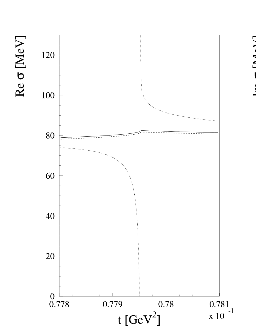
Figure 6: Real and imaginary parts of the scalar form factor as a function of $t$ at ${\cal O}(q^{3})$ in the vicinity of $t=4M_{\pi}^{2}$. Solid lines: EOMS scheme; dashed lines: infrared regularization (IR) of Ref. Becher:1999he ; dotted lines: HBChPT calculation of Ref. Bernard:1992qa . On this scale the (unphysical) divergence of both real and imaginary parts of the heavy-baryon result becomes visible.

Next we discuss the scalar form factor which is defined as

$$\langle N(p^{\prime})|\hat{m}[\bar{u}(0)u(0)+\bar{d}(0)d(0)]|N(p)\rangle=\bar{u}(p^{\prime})u(p)\sigma(t).$$

The numerical results for the real and imaginary parts of the scalar form factor at ${\cal O}(q^{4})$ are shown in Fig. 5 for the extended on-mass-shell scheme (solid lines) and the infrared regularization scheme (dashed lines). While the imaginary parts are identical in both schemes, the differences in the real parts are practically indistinguishable. Note that for both calculations $\sigma(0)$ and $\Delta_{\sigma}$ have been fitted to the dispersion results of Ref. Gasser:1990ce . Figure 6 contains an enlargement near $t\approx 4M_{\pi}^{2}$ for the results at ${\cal O}(p^{3})$ which clearly displays how the heavy-baryon calculation fails to produce the correct analytical behavior. Both real and imaginary parts diverge as $t\to 4M_{\pi}^{2}$.

As the final example, we consider the electromagnetic form factors of the nucleon which are defined via the matrix element of the electromagnetic current operator as

$$\langle N(p_{f})\left|J^{\mu}(0)\right|N(p_{i})\rangle=$$

$$\bar{u}(p_{f})\left[\gamma^{\mu}F_{1}^{N}(Q^{2})+\frac{i\sigma^{\mu\nu}q_{\nu}}{2m_{N}}F_{2}^{N}(Q^{2})\right]u(p_{i}),\,\,N=p,n,$$

where $q=p_{f}-p_{i}$ is the momentum transfer and $Q^{2}\equiv-q^{2}=-t\geq 0$. Instead of the Dirac and Pauli form factors $F_{1}$ and $F_{2}$ one commonly uses the electric and magnetic Sachs form factors $G_{E}$ and $G_{M}$ defined by

$$G^{N}_{E}(Q^{2}) = F^{N}_{1}(Q^{2})-\frac{Q^{2}}{4m_{N}^{2}}F_{2}^{N}(Q^{2}),$$

$$G^{N}_{M}(Q^{2}) = F^{N}_{1}(Q^{2})+F_{2}^{N}(Q^{2}).$$

At $Q^{2}=0$, these form factors are given by the electric charges and the magnetic moments in units of the charge and the nuclear magneton, respectively:

$$G_{E}^{p}(0)=1,\quad G_{E}^{n}(0)=0,\quad G_{M}^{p}(0)=1+\kappa_{p}=2.793,$$

$$G_{E}^{n}(0)=\kappa_{n}=-1.913.$$

Figure 7: The Sachs form factors of the nucleon at ${\cal O}(q^{4})$. The solid and dashed lines refer to the results in the EOMS scheme Fuchs:2003ir and the infrared regularization Kubis:2000zd , respectively. The experimental data for $G_{E}^{p}$, $G_{E}^{n}$, $G_{M}^{p}$, and $G_{M}^{n}$ are taken from Refs. GEP , GEN , GMP , and GMN , respectively.

Figure 7 shows the results for the Sachs form factors at ${\cal O}(q^{4})$ in the EOMS scheme (solid lines) Fuchs:2003ir and the infrared regularization (dashed lines) Kubis:2000zd . The description of $G_{E}^{p}$, $G_{M}^{p}$, and $G_{M}^{n}$ turns out to be only marginally better than that of the ${\cal O}(q^{3})$ calculation Fuchs:2003ir . For the very-small $Q^{2}$ region the improvement is due to additional free parameters which have been adjusted to the magnetic radii. As can be seen from Fig. 7, the ${\cal O}(q^{4})$ results only provide a decent description up to $Q^{2}=0.1\,\mbox{GeV}^{2}$ and do not generate sufficient curvature for larger values of $Q^{2}$. Moreover, the situation for $G_{E}^{n}$ seems to be even worse, where we found better agreement with the experimental data for the ${\cal O}(q^{3})$ results Fuchs:2003ir . We conclude that the perturbation series converges, at best, slowly and that higher-order contributions must play an important role.

6 Summary

We have discussed renormalization in the framework of mesonic and baryonic chiral perturbation theory. While the combination of dimensional regularization and the modified minimal subtraction scheme (of ChPT) leads to a straightforward power counting in terms of momenta and quark masses at a fixed ratio in the mesonic sector, the situation in the baryonic sector proves to be more complicated. At first sight, the correspondence between the loop expansion and the chiral expansion seems to be lost. Solutions to this problem have been given in terms of the heavy-baryon formulation and, more recently, the infrared regularization approach.

Here, we have discussed the so-called extended on-mass-shell renormalization scheme which allows for a simple and consistent power counting in the single-nucleon sector of manifestly Lorentz-invariant chiral perturbation theory. In this scheme a given diagram is assigned a chiral order $D$ according to Eq. (4). After reducing the diagram to the sum of dimensionally regularized scalar integrals multiplied by corresponding Dirac structures, one identifies, by expanding the integrands as well as the coefficients in small quantities, those terms which need to be subtracted in order to produce the renormalized diagram with the chiral order $D$ determined beforehand. Such subtractions can be realized in terms of local counterterms in the most general effective Lagrangian. Our approach may also be used in an iterative procedure to renormalize higher-order loop diagrams in agreement with the constraints due to chiral symmetry. Moreover, the EOMS renormalization scheme allows for implementing a consistent power counting in baryon chiral perturbation theory when vector (and axial-vector) mesons are explicitly included.

References

- (1) S. Weinberg, Physica A 96 (1979) 327.
- (2) J. Gasser and H. Leutwyler, Ann. Phys. (N.Y.) 158 (1984) 142; Nucl. Phys. B250 (1985) 465.
- (3) D. Issler, SLAC-PUB-4943-REV (1990) (unpublished); R. Akhoury and A. Alfakih, Ann. Phys. (N.Y.) 210 (1991) 81; S. Scherer and H. W. Fearing, Phys. Rev. D 52 (1995) 6445; H. W. Fearing and S. Scherer, Phys. Rev. D 53 (1996) 315; J. Bijnens, G. Colangelo, and G. Ecker, J. High Energy Phys. 9902 (1999) 020; T. Ebertshäuser, H. W. Fearing, and S. Scherer, Phys. Rev. D 65 (2002) 054033; J. Bijnens, L. Girlanda, and P. Talavera, Eur. Phys. J. C 23 (2002) 539.
- (4) J. Gasser, M. E. Sainio, and A. Švarc, Nucl. Phys. B307 (1988) 779.
- (5) A. Krause, Helv. Phys. Acta 63 (1990) 3.
- (6) G. Ecker and M. Mojžiš, Phys. Lett. B 365 (1996) 312.
- (7) U.-G. Meißner, G. Müller, and S. Steininger, Ann. Phys. (N.Y.) 279 (2000) 1.
- (8) N. Fettes, U.-G. Meißner, M. Mojžiš, and S. Steininger, Ann. Phys. (N.Y.) 283 (2001) 273 (2001); ibid. 288 (2001) 249.
- (9) J. Wess and B. Zumino, Phys. Lett. B 37 (1971) 95.
- (10) E. Witten, Nucl. Phys. B223 (1983) 422.
- (11) S. Weinberg, The Quantum Theory Of Fields. Vol. 1: Foundations (Cambridge University Press, Cambridge 1995).
- (12) E. Jenkins and A. V. Manohar, Phys. Lett. B 255 (1991) 558; ibid. 259 (1991) 353.
- (13) V. Bernard, N. Kaiser, J. Kambor, and U.-G. Meißner, Nucl. Phys. B388 (1992) 315.
- (14) S. Scherer, in Advances in Nuclear Physics, Vol. 27, edited by J. W. Negele and E. W. Vogt (Kluwer Academic/Plenum Publishers, New York 2003).
- (15) T. Becher and H. Leutwyler, Eur. Phys. J. C 9 (1999) 643.
- (16) G. ’t Hooft and M. J. Veltman, Nucl. Phys. B44 (1972) 189; M. J. Veltman, Diagrammatica. The Path to Feynman Rules (Cambridge University Press, Cambridge 1994).
- (17) S. Weinberg, Nucl. Phys. B363 (1991) 3.
- (18) G. Ecker, Prog. Part. Nucl. Phys. 35 (1995) 1.
- (19) T. Becher, in Proceedings of the Workshop Chiral Dynamics: Theory and Experiment III, Jefferson Laboratory, USA, 17 - 20 July, 2000, edited by A. M. Bernstein, J. L. Goity, and U.-G. Meißner (World Scientific, Singapore, 2002).
- (20) J. L. Goity, D. Lehmann, G. Prezeau, and J. Saez, Phys. Lett. B 504 (2001) 21; D. Lehmann and G. Prezeau, Phys. Rev. D 65 (2002) 016001.
- (21) J. Gegelia and G. Japaridze, Phys. Rev. D 60 (1999) 114038.
- (22) T. Fuchs, J. Gegelia, G. Japaridze, and S. Scherer, hep-ph/0302117; to appear in Phys. Rev. D.
- (23) H.-B. Tang, hep-ph/9607436; P. J. Ellis and H.-B. Tang, Phys. Rev. C 57 (1998) 3356; M. F. Lutz, Nucl. Phys. A677 (2000) 241; M. F. Lutz and E. E. Kolomeitsev, Nucl. Phys. A700 (2002) 193.
- (24) J. Gegelia, G. S. Japaridze, and K. S. Turashvili, Theor. Math. Phys. 101 (1994) 1313.
- (25) T. Fuchs, M. R. Schindler, J. Gegelia, and S. Scherer, hep-ph/0308006.
- (26) M. R. Schindler, J. Gegelia, and S. Scherer, hep-ph/0309005.
- (27) T. Becher and H. Leutwyler, J. High Energy Phys. 0106 (2001) 017.
- (28) R. Koch, Nucl. Phys. A448 (1986) 707.
- (29) J. Gasser, H. Leutwyler, and M. E. Sainio, Phys. Lett. B 253 (1991) 252.
- (30) T. P. Cheng and R. F. Dashen, Phys. Rev. Lett. 26 (1971) 594.
- (31) L. S. Brown, W. J. Pardee, and R. D. Peccei, Phys. Rev. D 4 (1971) 2801.
- (32) T. Fuchs, J. Gegelia, and S. Scherer, nucl-th/0305070.
- (33) B. Kubis and U.-G. Meißner, Nucl. Phys. A679 (2001) 698.
- (34) L. E. Price, J. R. Dunning, M. Goitein, K. Hanson, T. Kirk, and R. Wilson, Phys. Rev. D 4 (1971) 45; C. Berger, V. Burkert, G. Knop, B. Langenbeck, and K. Rith, Phys. Lett. B 35 (1971) 87; K. M. Hanson, J. R. Dunning, M. Goitein, T. Kirk, L. E. Price, and R. Wilson, Phys. Rev. D 8 (1973) 753; G. G. Simon, C. Schmitt, F. Borkowski, and V. H. Walther, Nucl. Phys. A333 (1980) 381.
- (35) T. Eden et al., Phys. Rev. C 50 (1994) 1749; I. Passchier et al., Phys. Rev. Lett. 82 (1999) 4988; M. Ostrick et al., Phys. Rev. Lett. 83 (1999) 276; C. Herberg et al., Eur. Phys. J. A 5 (1999) 131; J. Becker et al., Eur. Phys. J. A 6 (1999) 329.
- (36) T. Janssens, R. Hofstadter, E. B. Hughes, and M. R. Yearian, Phys. Rev. 142 (1966) 922; C. Berger, V. Burkert, G. Knop, B. Langenbeck, and K. Rith, Phys. Lett. B 35 (1971) 87; K. M. Hanson, J. R. Dunning, M. Goitein, T. Kirk, L. E. Price, and R. Wilson, Phys. Rev. D 8 (1973) 753; G. Höhler, E. Pietarinen, I. Sabba Stefanescu, F. Borkowski, G. G. Simon, V. H. Walther, and R. D. Wendling, Nucl. Phys. B114 (1976) 505.
- (37) P. Markowitz et al., Phys. Rev. C 48 (1993) 5; H. Anklin et al., Phys. Lett. B 336 (1994) 313; E. E. Bruins et al., Phys. Rev. Lett. 75 (1995) 21; H. Anklin et al., Phys. Lett. B 428 (1998) 248; W. Xu et al., Phys. Rev. Lett. 85 (2000) 2900; G. Kubon et al., Phys. Lett. B 524 (2002) 26.