ABSTRACT

We review the effective Lagrangian of the Higgs penguin in the Standard Model and its minimal supersymmetric extension (MSSM). As a master application of the Higgs penguin, we discuss in some detail the B-meson decays into a lepton-antilepton pair. Furthermore, we explain how this can probe the Higgs sector of the MSSM provided that some of these decays are seen at Tevatron Run II and B-factories. Finally, we present a complete list of observables where the Higgs penguin could be strongly involved.

1 Prologue

Glashow and Weinberg in their seminal paper [1] pointed out that Flavour Changing Neutral Currents (FCNC) are suppressed “naturally” if all the down-type quarks acquire their masses through their coupling to the same Higgs boson doublet, say $H_{d}$, and all the up-type quarks through their coupling to a second Higgs boson doublet, say $H_{u}$. These two doublets may [Standard Model (SM) case] or may not [Two Higgs doublet Model type-II (2HDM) case] be charge conjugates of each other. In general, if no symmetry considerations are assumed at tree level, a departure from the above rule leads to severe enhancement of $K-\overline{K}$ and/or $B-\overline{B}$ mixing not seen at the experimental data [2]. In the Minimal Supersymmetric Standard Model (MSSM) the Glashow-Weinberg scheme is naturally realized due to the holomorphicity of the superpotential; Higgs FCNC processes appear only at loop level when the holomorphicity is violated by finite radiative threshold corrections due to the soft SUSY breaking interactions[3]. In this brief review, we shall present the effective Lagrangian of the Higgs boson FCNC’s in the SM and MSSM, which we term “Higgs penguins”, and discuss their significance in B-, K-meson and $\tau$-lepton physics.

2 The Higgs penguin

The term “Higgs penguin” is used here in analogy to the well known Z-penguin, to denote $H-f-f^{\prime}$ loop induced flavour transitions, where $f,f^{\prime}$ are either quarks or leptons. For B- or K-physics experiments, the relevant Higgs penguin is the one with down quarks $(f=d)$ in the external legs, drawn schematically in Fig.1.

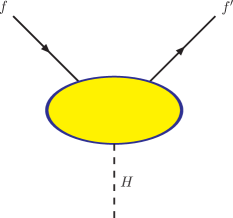
Figure 1: The Higgs penguin. The blob consists of loop corrections due to Standard or Beyond the Standard Model particles.

2.1 The Standard Model Higgs penguin

The flavour changing Higgs vertex $H-d-d^{\prime}$ in the SM was first calculated in [4, 5]. It came rather as a surprise to observe that the coupling of the resulting Higgs $H-d-d^{\prime}$ penguin vertex is proportional to $m_{d(d^{\prime})}/M_{W}$ instead of being suppressed by $(m_{d(d^{\prime})}/M_{W})^{3}$. Denoting the up and down $3\times 3$ diagonal quark mass matrices with ${\bf\hat{M}_{u}}$ and ${\bf\hat{M}_{d}}$, and with ${\bf{V}}$ the Cabbibo-Kobayashi-Maskawa (CKM) matrix, the SM one-loop effective Lagrangian for quark flavour changing interactions with the Higgs boson reads

$${\cal L}^{\rm SM}_{H\bar{d}d^{\prime}}\ =\ -\,\frac{g_{w}}{2M_{W}}\,H\>\bar{d}\,\Big{(}\,{\bf\hat{M}_{d}}\,{{\bf g}}_{H\bar{d}d^{\prime}}^{L}\,P_{L}\ +\ {{\bf g}}_{H\bar{d}d^{\prime}}^{R}\,{\bf\hat{M}_{d^{\prime}}}P_{R}\,\Big{)}\,d^{\prime}\,,$$ (2.1)

where $P_{L\,(R)}=[1-(+)\,\gamma_{5}]/2$, and

$${{\bf g}}_{H\bar{d}d^{\prime}(d\neq d^{\prime})}^{L}\>\!\!=\!\!\>-\frac{3}{4}\>\frac{g_{w}^{2}}{(16\pi^{2})}\>{\bf{V}}^{\dagger}\>\frac{{\bf\hat{M}_{u}}^{2}}{M_{W}^{2}}\>{\bf{V}}\;\;\;\;,\;\;\;\;{{\bf g}}_{H_{i}\bar{d}d^{\prime}}^{R}\!\! = \!\!\big{(}\,{{\bf g}}_{H_{i}\bar{d}d^{\prime}}^{L}\,\big{)}^{\dagger}\,.$$ (2.2)

The tree level flavour diagonal quark Higgs couplings are ${{\bf g}}_{H_{i}\bar{d}d}^{R}=\big{(}\,{{\bf g}}_{H_{i}\bar{d}d}^{L}\,\big{)}^{\dagger}={\bf 1}$. For this calculation the masses and the momenta of the external particles have been set to zero. This simple result arises from the sum of 10 diagrams in $R_{\xi}$ gauge (6 Higgs penguins and 4 self energy diagrams) shown in Fig.(2).

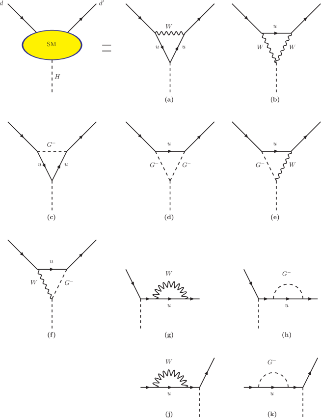
Figure 2: SM contributions to the Higgs penguin. The label $u$ denotes all the up-type quarks $(u,c,t)$, and $G^{\pm}$ the charged Goldstone modes.

In a general $R_{\xi}$ gauge, the diagrams (c),(e),(f),(g),(h),(j),(k) are divergent. The Glashow-Iliopoulos-Maiani (GIM) mechanism [6] removes divergences from diagrams (e) and (f) aswell as from (g) and (j). The remaining divergences in diagrams (c), (h) and (k) cancel each other and the finite sum, in the case of a constant background Higgs field, is given in Eqs.(2.1,2.2). Although it seems straightforward to calculate the 10 diagrams in Fig.(2), it took many years for gauge dependencies and renormalization scheme ambiguities to be clarified in the literature. The result of Refs.[4, 5] given in Eqs.(2.1,2.2) was finally confirmed by several groups [7, 8, 9, 10, 11, 12, 13, 14] and different methods.

For $B_{d}$- or $B_{s}$-meson initial state ($d\equiv b$ and $d^{\prime}\equiv d\,~{}{\rm or}~{}\,s$), the dominant contribution in Eq.(2.2) comes from the top quark in the loop while for Kaon initial state ($d\equiv s$ and $d^{\prime}\equiv d$) it comes from the charm quark in the loop. Comparing the Higgs penguin prefactor of Eq.(2.1) and Eq.(2.2) to the Z-boson penguin ($d\>Z_{\mu}\>d^{\prime}$) one in Ref. [15], we obtain that the former is about $m_{d}/M_{W}$ times smaller than the latter, with $m_{d}$ being the mass of the heaviest external quark.

2.2 The Supersymmetric Higgs penguin

For the construction of the supersymmetric version of the SM Higgs penguin two approaches have been devised: the Feynman diagrammatic approach and the Effective Lagrangian approach. Both have advantages and disadvantages and it is worth describing briefly both approaches here.

2.2.1 Feynman Diagrammatic Approach

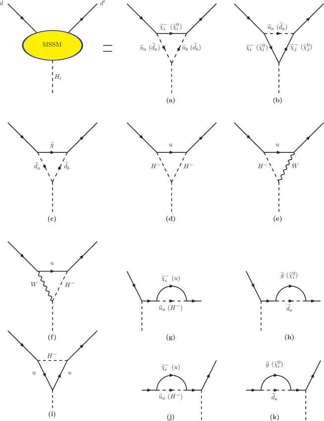
Figure 3: General and complete MSSM contributions to the Higgs penguin. The labels $\widetilde{u},\widetilde{d}$ denote all flavours for up and down type squarks with a=1,2 being their mass eigenstates. Charginos are labeled with $\widetilde{\chi}_{i}^{-},i=1,2$, neutralinos with $\widetilde{\chi}_{i}^{0},i=1...4$ and the gluino with $\widetilde{g}$. $H^{\pm}$ is the charged Higgs boson.

This approach is a straightforward (but somehow tedious) calculation of the diagrams shown in Fig.(3). It needs to be supplemented with the so called $\tan\beta$-resummation procedure. The main advantage is that within this approach effects beyond the $SU(2)\times U(1)$ limit are automatically included. This approach has been followed by various groups (usually through a specific application) [17, 18, 19, 20, 21, 22, 23]. The 17 diagrams in Fig.(3) are just supersymmetrizations of the SM diagrams in Fig.(2). To our knowledge they have not yet been calculated in full detail . The latest calculation [19] is restricted only to results that have been derived in the large $\tan\beta$ approximation with the low $\tan\beta$ regime remaining unexplored although one does not expect dramatic effects for heavy (TeV) supersymmetric particles. Some remarks on the diagrams in Fig.(3) are in order here: i) the bulk of the corrections to the Higgs penguin arise just from the finite part of the self energies (g,j) with charginos and up-squarks in the loop; they scale like $\tan^{2}\beta$. They do not vanish even (and especially) in the case of degenerate squark masses, and the MSSM corrections to the Higgs penguin do not decouple even if the squark masses are at multi-TeV scale. Diagrams (d),(e),(f),(i),(g) and (j) with the charged Higgs boson (two Higgs doublet model contributions  [24, 25, 19] ) are also non zero but are subdominant since they scale like $\tan\beta$. Ultraviolet Infinities of the diagrams (g,j) cancel against the vertex diagram (b). ii) Diagrams (a),(b),(c),(h) and (k) with neutralinos or gluinos and squarks in the loop arise only for non degenerate squark spectrum due to renormalization group running effects or Planck scale squark flavour changing insertions. In this case, the gluino contributions can compete with the chargino ones and even cancel each other (this will be clear in a minute). The neutralino diagrams in (a,b,h,k) play rather a subdominant role except for the case of the exact cancellation of the gluino and chargino contributions [20]. iii) Within the Feynman diagrammatic approach, $\tan\beta$-resummation effects have been added in Ref.[21] for all diagrams in Fig.(3) apart from the gluino and neutralino ones. In addition, SUSY CP-violating effects were taken into account in [22].

2.2.2 Effective Lagrangian Approach

This approach allows for a simpler derivation of the dominant corrections to the Higgs penguin (including resummation of $\tan\beta$) in the large $\tan\beta\lower 3.01385pt\hbox{$\;\stackrel{{\scriptstyle\textstyle>}}{{\sim}}\;$}40$ regime but can not easily implement $SU(2)\times U(1)$ electroweak symmetry breaking effects which are relevant for small values of $\tan\beta$. This approach has been followed in Refs. [26, 27, 28, 29, 30, 31, 32]. The general resummed Higgs penguin, which includes CP-violating effects in the MSSM, is given by [30]:

$${\cal L}_{H_{i}\bar{d}d^{\prime}}\ =\ -\,\frac{g_{w}}{2M_{W}}\,\sum_{i=1}^{3}\,H_{i}\>\bar{d}\,\Big{(}\,{\bf\hat{M}_{d}}\,{{\bf g}}_{H_{i}\bar{d}d^{\prime}}^{L}\,P_{L}\ +\ {{\bf g}}_{H_{i}\bar{d}d^{\prime}}^{R}\,{\bf\hat{M}_{d^{\prime}}}P_{R}\,\Big{)}\,d^{\prime}\,,$$ (2.5)

in the notation of Eq.(2.1), with

$${{\bf g}}_{H_{i}\bar{d}d^{\prime}\>(d\neq d^{\prime})}^{L}\!\! = \!\!{\bf{V}}^{\dagger}{\bf{R}}^{-1}{\bf{V}}\,\Biggl{[}\frac{O_{1i}}{\cos\beta}\ -\ \frac{O_{2i}}{\sin\beta}\ +\ \frac{i\>O_{3i}}{\sin\beta\>\cos\beta}\,\Biggr{]}\,,\quad{{\bf g}}_{H_{i}\bar{d}d^{\prime}}^{R}\!\!=\!\!\big{(}\,{{\bf g}}_{H_{i}\bar{d}d^{\prime}}^{L}\,\big{)}^{\dagger}\,,$$ (2.6)

where ${\bf{R}}$ is the $3\times 3$ dimensional mass matrix which resums all the $\tan\beta$ enhanced finite threshold effects. It is given by :

$${\bf{R}}\ =\ {\bf 1}\>+\>{\bf{E}_{g}}\tan\beta\>+\>{\bf{E}_{u}}\tan\beta\,|{\bf\hat{h}_{u}}|^{2}\>+\>\dots\;,$$ (2.7)

where ${\bf\hat{h}_{u}}$ is the diagonal up-Yukawa couplings, and up to small corrections is : ${\bf\hat{h}_{u}}=\frac{\sqrt{2}\>{\bf\hat{M}_{u}}}{v_{2}}$. Furthermore, $O_{ij}$ is a $3\times 3$ orthogonal matrix, which transforms the Higgs boson fields from their weak to their mass eigenstates and accounts for the CP-violating Higgs mixing effects [33]. In addition, ${\bf{E}_{g}}$ and ${\bf{E}_{u}}$ are finite threshold effects induced by the diagrams in Fig.(4). The ellipses in (2.7) denote additional (generically sub-dominant) threshold effects like, for example, the bino-wino contribution which corresponds to the neutralino contribution diagram in Fig.(3).

Figure 4: Non-holomorphic radiative effects on the down-quark Yukawa couplings of the form $[{\bf h_{d}}\>d_{L}\Phi_{2}^{0*}d_{R}]$ induced by (a) gluinos and (b) higgsinos. The Higgs field $\Phi_{2}^{0}$ is the one which couples to the up-type quarks in the superpotential, i.e., $[{\bf h_{u}}\>u_{L}\Phi_{2}^{0}u_{R}]$. From Ref.[30].

${\bf{E}_{g}}$ and ${\bf{E}_{u}}$ are in general complex $3\times 3$ matrices but, for simplicity, here we will assume that they are diagonal (the reader may consult Ref.[30] for more details at this point) :

$${\bf\hat{E}_{g}} = {\bf 1}\,\frac{2\alpha_{s}}{3\pi}\,m_{\tilde{g}}^{*}\mu^{*}\,I(m_{\tilde{d}_{L}}^{2},m_{\tilde{d}_{R}}^{2},|m_{\tilde{g}}|^{2})\stackrel{{\scriptstyle M_{\rm SUSY}\gg M_{W}}}{{\longrightarrow}}{\bf 1}\,\frac{\alpha_{s}}{3\pi}\>e^{-i\>(\phi_{\mu}+\phi_{g})}\;,$$ (2.8)

$${\bf\hat{E}_{u}} = {\bf 1}\,\frac{1}{16\pi^{2}}\,\mu^{*}A_{U}^{*}\,I(m_{\tilde{u}_{L}}^{2},m_{\tilde{u}_{R}}^{2},|\mu|^{2})\stackrel{{\scriptstyle M_{\rm SUSY}\gg M_{W}}}{{\longrightarrow}}{\bf 1}\,\frac{1}{32\pi^{2}}\>e^{-i\>(\phi_{\mu}+\phi_{A_{U}})}\;.$$ (2.9)

The limit in Eqs.(2.8,2.9) is at degenerate supersymmetric masses, $M_{SUSY}\equiv|m_{\tilde{g}}|=|\mu|=m_{\tilde{d}_{L}}=m_{\tilde{d}_{R}}=|A_{U}|=m_{\tilde{u}_{L}}=m_{\tilde{u}_{R}}$ and $\phi_{\mu},\phi_{g},\phi_{A_{U}}$ are the phases of the higgsino mixing parameter $\mu$, the gluino mass $m_{\tilde{g}}$, and the trilinear supersymmetry breaking coupling $A_{U}$, respectively. The loop integral $I(x,y,z)$ is given in [30]. Even in this limit, $M_{\rm SUSY}\gg M_{W}$ a nightmare scenario for the LHC, the Higgs penguin amplitude remains significant and does not decouple; it depends on the various CP-violating phases and details of the Higgs sector [mixing matrix $(O_{ij})$] and the experimentally nearly-known quark sector.

Equations (2.5,2.6,2.7) represent the Higgs penguin amplitude in the MSSM. In order to qualitatively understand the behaviour of the MSSM Higgs penguin, it is instructive to take the limit of large $\tan\beta$, i.e., $1/\cos\beta\simeq\tan\beta,\;\sin\beta\simeq 1$ and apply the limits (2.8,2.9) in Eqs.(2.5,2.6,2.7). Then, we obtain:

$${{\bf g}}_{H_{i}\bar{d}d^{\prime}\>(d\neq d^{\prime})}^{L}\!\!=\!\!-\frac{1}{4}\>\frac{g_{w}^{2}}{(16\pi^{2})}\>{\bf{V}}^{\dagger}\Big{(}\frac{{\bf\hat{M}_{u}}^{2}}{M_{W}^{2}}\Big{)}\>\times$$

$$\frac{\Big{(}O_{1i}+i\>O_{3i}\Big{)}\>e^{-i(\phi_{\mu}+\phi_{A_{U}})}\>\tan^{2}\beta}{\Big{[}{\bf 1}+\frac{\alpha_{s}}{3\pi}\>e^{-i(\phi_{\mu}+\phi_{g})}\>\tan\beta\Big{]}\>\Big{[}{\bf 1}+\Big{(}\frac{\alpha_{s}}{3\pi}\>e^{-i(\phi_{\mu}+\phi_{g})}\>+\>\frac{g_{w}^{2}}{64\pi^{2}}\frac{{\bf\hat{M}_{u}}^{2}}{M_{W}^{2}}\>e^{-i(\phi_{\mu}+\phi_{A_{U}})}\Big{)}\>\tan\beta\Big{]}}\>{\bf{V}}\;,$$

$${{\bf g}}_{H_{i}\bar{d}d^{\prime}}^{R}\!\!=\!\!\big{(}\,{{\bf g}}_{H_{i}\bar{d}d^{\prime}}^{L}\,\big{)}^{\dagger}\,.$$ (2.10)

By looking at Eq.(2.2.2), we conclude the following :

• The MSSM Higgs penguin is enhanced by two powers of $\tan\beta$ with respect to the SM one. Compare Eqs (2.2.2) and (2.2).

• The MSSM Higgs penguin is in general a complex number due to the additional supersymmetric CP-violating phases, $\phi_{A_{U}}$, $\phi_{\mu}$. In the CP-invariant limit the coupling ${{\bf g}}_{H_{i}\bar{d}d^{\prime}\>(d\neq d^{\prime})}^{L}$ is either pure real or pure imaginary.

• The MSSM Higgs penguin’s largest correction, Eq.(2.9), depends on the soft supersymmetry breaking trilinear parameter, $A_{U}$. Therefore, it is enhanced only in the case of the maximal stop-mixing case, $A_{t}\lower 3.01385pt\hbox{$\;\stackrel{{\scriptstyle\textstyle>}}{{\sim}}\;$}M_{W}$, which is favoured also by MSSM Higgs searches.

• The limit $\big{[}{\bf 1}+{\bf{E}_{g}}\tan\beta\big{]}\rightarrow 0$ in the master formula Eq.(2.6), or equivalent the approximation $\big{[}{\bf 1}+\frac{\alpha_{s}}{3\pi}\>e^{-i(\phi_{\mu}+\phi_{g})}\>\tan\beta\big{]}\rightarrow 0$ in Eq.(2.2.2), is attainable and not singular. In this limit the Higgs penguin diagram goes to a constant value (and not to infinity) due to the GIM mechanism. This is a result of the general resummed effective Lagrangian, equipped in [30], that integrates and improves earlier constructions [26, 27, 28, 29].

• The MSSM Higgs penguin will dominate over all the box- or penguin-type supersymmetric contributions to the physical observables since the latter vanish due to the super GIM mechanism in the limit of the degenerate squark masses [34, 35].

• The resummation matrix ${\bf R}$ controls the strength of the Higgs-mediated FCNC effects. For instance, if ${\bf R}$ is proportional to unity, then a kind of a GIM-cancellation mechanism becomes operative and the Higgs-boson contributions to all FCNC observables vanish identically. Furthermore, not only the top quark, but also the other up-type quarks can give significant contributions to FCNC transition amplitudes, which are naturally included in (2.5) through the resummation matrix ${\bf R}$. All these effects are computed explicitly within physical observables in Ref.[30].

• The Lagrangian in Eq.(2.5) captures the bulk of the full corrections of Fig.(3) at large $\tan\beta\lower 3.01385pt\hbox{$\;\stackrel{{\scriptstyle\textstyle>}}{{\sim}}\;$}40$ and is limited for supersymmetric breaking masses $M_{\rm SUSY}$ much heavier than the electroweak scale. Additional electroweak corrections (after the $SU(2)\times U(1)$ gauge symmetry breaking) have been calculated in [31].

We will now turn to the physical applications of the Higgs penguin.

3 Applications

There is a vast amount of applications one can think of. Basically, the Higgs penguin participates in those physical observables where the Z-penguin does so. In this section we shall discuss, in a rather qualitative way, the effect of the Higgs penguin $[H-b-d(s)]$ on B-, K-meson and $\tau$-lepton physics observables. The models under consideration will be the Standard model and its minimal supersymmetric extension, MSSM, with R-parity symmetry.

3.1 The Master Application : $\bar{B}_{q}\rightarrow l^{+}l^{-}$ and implications

It is rather compulsory to discuss first the $B_{q}$-meson ($q=d,s$) decay to a lepton ($l=e,\mu,\tau$) pair. The decay $\bar{B}_{q}\rightarrow l^{+}l^{-}$ is mediated by the Higgs penguin, the Z-penguin and box diagrams[15]. It has been extensively discussed in the literature, both in the SM [36] and in the MSSM [37] case (for other models see Ref.[47]). None of the processes $\bar{B}_{q}\rightarrow l^{+}l^{-}$ have been seen so far, and the experimental bounds on these “very rare” B-decays are listed in Table 1.

${\cal B}$(Channel)	Expt.	Bound (90% CL)	SM prediction
$B_{s}\to e^{+}e^{-}$	L3 [48]	$<5.4\times 10^{-5}$	$(8.9\pm 2.3)\times 10^{-14}$
$B_{s}\to\mu^{+}\mu^{-}$	CDF [49]	$<9.5\times 10^{-7}$	$(3.8\pm 1.0)\times 10^{-9}$
$B_{s}\to\tau^{+}\tau^{-}$	LEP [50]	$<0.05$	$(8.2\pm 2.1)\times 10^{-7}$
$B_{d}\to e^{+}e^{-}$	Belle [51]	$<1.9\times 10^{-7}$	$(2.4\pm 1.4)\times 10^{-15}$
$B_{d}\to\mu^{+}\mu^{-}$	Belle [51]	$<1.6\times 10^{-7}$	$(1.0\pm 0.6)\times 10^{-10}$
$B_{d}\to\tau^{+}\tau^{-}$	LEP [50]	$<0.015$	$(2.1\pm 1.2)\times 10^{-8}$

Table 1: The experimental status and the SM predictions for the branching ratios ${\cal B}$($\bar{B}_{q}\rightarrow l^{+}l^{-}$ ). The error in the $B_{s}$ branching ratios mainly originates from the uncertainty in $f_{B_{s}}=230\pm 30$ MeV [52], and the error in the $B_{d}$ branching ratios corresponds to the uncertainties in $f_{B_{d}}=200\pm 30$ MeV [52] and $|V_{td}|=0.040\pm 0.002$ linearly added. This is the updated version of the Table 1 presented in Ref.[38].

The decays $\bar{B}_{q}\rightarrow l^{+}l^{-}$ are interesting probes of physics beyond the SM since the best bound we have so far, that on ${\cal B}(B_{s}\rightarrow\mu^{+}\mu^{-})$, is three orders of magnitude away from the SM expectation [40]. In addition, the decay $B_{s,d}\rightarrow\mu^{+}\mu^{-}$ is one of the experimentally favoured and has a bright future : Tevatron Run II with luminosity of 2 ${\rm fb}^{-1}$ has a single event sensitivity [53] of ${\cal B}(B_{s}\rightarrow\mu^{+}\mu^{-})=1.0\times 10^{-8}$ (the background from Run I is roughly one event): 10 events at CDF with ${\cal L}=2~{}{\rm fb}^{-1}$ means a ${\cal B}(B_{s}\rightarrow\mu^{+}\mu^{-})\simeq 10^{-7}$. A recent analysis [54, 41] showed that CDF can discover $B_{s}\rightarrow\mu^{+}\mu^{-}$ in Run IIb with an integrated luminosity of 15 ${\rm fb}^{-1}$ if ${\cal B}(B_{s}\rightarrow\mu^{+}\mu^{-})\lower 3.01385pt\hbox{$\;\stackrel{{\scriptstyle\textstyle>}}{{\sim}}\;$}10^{-8}$. If ${\cal B}(B_{s}\rightarrow\mu^{+}\mu^{-})$ turns out to be SM-like (see Table 1), then only LHC will be able to measure it [55].

Motivated by the above discussion, we are now going to see why and how one can achieve branching ratios for the decays $\bar{B}_{q}\rightarrow l^{+}l^{-}$ that could appear soon at the Tevatron and B-factories. To this end, we shall follow the effective Lagrangian technique employed in Ref. [30]. Neglecting contributions proportional to the lighter quark masses $m_{d,s}$, the relevant effective Hamiltonian for $\Delta B=1$ FCNC transitions, such as $b\to q\ell^{+}\ell^{-}$ with $q=d,s$, is given by

$$H_{\rm eff}^{\Delta B=1}\ =\ -\,\frac{4\>G_{F}}{\sqrt{2}}\,V_{tb}V_{tq}^{*}\,\Big{(}\,C_{S}\,{\cal O}_{S}\ +\ C_{P}\,{\cal O}_{P}\ +\ C_{10}\,{\cal O}_{10}\Big{)}\;,$$ (3.11)

where

$${\cal O}_{S} = \frac{e^{2}}{16\pi^{2}}\,m_{b}\,(\bar{q}P_{R}b)\,(\bar{\ell}\ell)\;,$$

$${\cal O}_{P} = \frac{e^{2}}{16\pi^{2}}\,m_{b}\,(\bar{q}P_{R}b)\,(\bar{\ell}\gamma_{5}\ell)\;,$$

$${\cal O}_{10} = \frac{e^{2}}{16\pi^{2}}\,(\bar{q}\gamma^{\mu}P_{L}b)\,(\bar{\ell}\gamma_{\mu}\gamma_{5}\ell)\;.$$ (3.12)

By making use of our master resummed Higgs penguin effective Lagrangian Eq.(2.5,2.6,2.7), the Wilson coefficients $C_{S}$ and $C_{P}$ (in the region of large values of $\tan\beta$) read:

$$C_{S} = \frac{2\pi m_{\ell}}{\alpha_{\rm em}}\,\frac{1}{V_{tb}V_{tq}^{*}}\,\sum_{i=1}^{3}\,\frac{g_{H_{i}\bar{q}b}^{R}\,g_{H_{i}\bar{\ell}\ell}^{S}}{M_{H_{i}}^{2}}\ ,$$

$$C_{P} = i\,\frac{2\pi m_{\ell}}{\alpha_{\rm em}}\,\frac{1}{V_{tb}V_{tq}^{*}}\,\sum_{i=1}^{3}\,\frac{g_{H_{i}\bar{q}b}^{R}\,g_{H_{i}\bar{\ell}\ell}^{P}}{M_{H_{i}}^{2}}\ ,$$ (3.13)

with $C_{10}=-\frac{1}{\sin^{2}\theta_{w}}(\frac{\overline{m}_{t}(m_{t})}{167~{}{\rm GeV}})^{1.55}\simeq 4.3$ [36] and $\overline{m}_{t}(m_{t})$ the running $\overline{MS}$ top quark mass. $M_{H_{i}}$ denotes the neutral Higgs boson masses, $M_{H_{1}}<M_{H_{2}}\lower 3.01385pt\hbox{$\;\stackrel{{\scriptstyle\textstyle<}}{{\sim}}\;$}M_{H_{3}}$. $C_{10}$ is actually the dominant contribution in the SM case and originates from the Z-boson penguin and the box diagrams [15]. In addition, the reduced scalar and pseudoscalar Higgs couplings to charged leptons $g_{H_{i}\bar{\ell}\ell}^{S,P}$ in Eqs.(3.1) are given by [30, 56]

$$g_{H_{i}\bar{\ell}\ell}^{S}\ =\ \frac{O_{1i}}{\cos\beta}\ ,\qquad g_{H_{i}\bar{\ell}\ell}^{P}\ =\ -\,\tan\beta\,O_{3i}\;,$$ (3.14)

where loop vertex effects on the leptonic sector have been omitted as being negligibly small. The reader must have already noticed that, at the large $\tan\beta$ regime, we have $g_{H_{i}\bar{\ell}\ell}^{S}\simeq O_{1i}\times\tan\beta$ and thus from Eqs.(2.2.2,3.1,3.14) we obtain that the scalar and pseudoscalar Wilson coefficients $C_{S,P}$ grow like $\tan^{3}\beta$. The branching ratio for the $\bar{B}^{0}_{q}$ meson decay to $\ell^{+}\ell^{-}$ acquires the simple form [19, 24]

$${\cal B}(\bar{B}^{0}_{q}\to\ell^{+}\ell^{-}) =$$

$$\frac{G_{F}^{2}\alpha_{\rm em}^{2}}{16\pi^{3}}\,M_{B_{q}}\tau_{B_{q}}\,|V_{tb}V_{tq}^{*}|^{2}\,\sqrt{1-\frac{4m_{\ell}^{2}}{M_{B_{q}}^{2}}}\ \Bigg{[}\,\Bigg{(}\,1-\frac{4m_{\ell}^{2}}{M_{B_{q}}^{2}}\Bigg{)}\,|F^{q}_{S}|^{2}\ +\ |F_{P}^{q}\>+\>2m_{\ell}F_{A}^{q}|^{2}\,\Bigg{]}\;,$$

where $\tau_{B_{q}},M_{B_{q}}$ is the total lifetime and the mass of the $B_{q}$ meson, respectively, and

$$F_{S,P}^{q}\ =\ -\,\frac{i}{2}\,M_{B_{q}}^{2}f_{B_{q}}\,\frac{m_{b}}{m_{b}+m_{q}}\,C_{S,P}\;,\qquad F_{A}^{q}\ =\ -\,\frac{i}{2}\,f_{B_{q}}\,C_{10}\;.$$ (3.16)

$F_{S,P}$ is roughly $(m_{b}^{2}/M_{W}^{2})\tan^{3}\beta$ times bigger than $F_{A}$ and thus dominate for large values of $\tan\beta$. Other electroweak SUSY box and Z-penguin contributions grow with at most two powers of $\tan\beta$ and thus are subdominant in this region. Numerical values for the parameters entering Eq.(3.1,3.16) can be found in PDG [2] and in the caption of Table (1). The Higgs matrix elements [$O_{ij}$] in the MSSM can be obtained from the numerical code CPsuperH[56]. In general, we have $O_{11},O_{31}\ll 1$, and thus from Eqs.(3.1) we conclude that the ratio ${\cal B}(B_{q}\rightarrow l^{+}l^{-})$ depends only on the heaviest Higgs boson mass, $M_{H_{3}}$. In the simple case of equal squark masses, and by employing Eqs.(2.2.2,3.1,3.14,3.1,3.16), the reader can convince himself that the experimental bounds in Table 1 are attainable in the MSSM. In general cases of squark non-degeneracy one should use the master formula given in Eqs.(2.5,2.6).

3.1.1 Implications: probing the Higgs sector with $B_{s,d}\rightarrow\mu^{+}\mu^{-}$ at Tevatron and B-factories

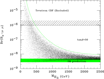
Figure 5: The ${\cal B}(B_{s}\rightarrow\mu^{+}\mu^{-})$ vs. the Heaviest Higgs boson mass in the MSSM for $\tan\beta=50$ and $m_{t}=175$ GeV. The shaded area shows the SM prediction for ${\cal B}(B_{s}\rightarrow\mu^{+}\mu^{-})$ (see Table 1). The excluded area from Tevatron CDF [49] is also displayed.

As we show, in the MSSM ${\cal B}(B_{s}\rightarrow\mu^{+}\mu^{-})$ is enhanced by six powers of $\tan\beta$ and suppressed by four powers of the heaviest Higgs boson mass, $M_{H_{3}}$. On the other hand, $\tan\beta$ has a theoretical upper bound (around 50) coming from the perturbativity of the Yukawa couplings up to the Grand Unification (GUT) scale. Therefore, we can use a future possible evidence for $B_{s}\rightarrow\mu^{+}\mu^{-}$ to set an upper bound on $M_{H_{3}}$. Having all the machinery at hand from the previous section, we do this exercise here. In order to illustrate our argument, let us envision the following situation:

• Tevatron Run II finds $B_{s}\rightarrow\mu^{+}\mu^{-}$

• BaBar and Belle (or a high luminosity upgraded B-factory) confirm the equation ${\cal B}(B_{d}\rightarrow\mu^{+}\mu^{-})\simeq|\frac{V_{td}}{V_{ts}}|^{2}{\cal B}(B_{s}\rightarrow\mu^{+}\mu^{-})$, and no indication is found for non-minimal flavour structure

What do these hypothetical facts imply? We can use a high statistics scan over the MSSM parameter space in the region where the soft breaking masses are below 2.5 TeV and the trilinear couplings below $|A|\lower 3.01385pt\hbox{$\;\stackrel{{\scriptstyle\textstyle<}}{{\sim}}\;$}5$ TeV. We assume that the Lightest Supersymmetric particle (LSP) is stable and require it to be neutral. No new flavour structure other than the CKM is assumed. Under these assumptions, we plot in Fig.(5) ${\cal B}(B_{s}\rightarrow\mu^{+}\mu^{-})$ vs. $M_{H_{3}}$. The envelope contour is well approximated by

$${\cal B}(B_{s}\rightarrow\mu^{+}\mu^{-}) = 5\times 10^{-7}~{}\biggl{(}\frac{\tan\beta}{50}\biggr{)}^{6}~{}\biggl{(}\frac{550~{}{\rm GeV}}{M_{H_{3}}}\biggr{)}^{4}+8\times 10^{-9}\;.$$ (3.17)

If CDF Run IIa sees 50 events for the $B_{s}\rightarrow\mu^{+}\mu^{-}$ [that means ${\cal B}(B_{s}\rightarrow\mu^{+}\mu^{-})\simeq 5\times 10^{-7}$] then $M_{H_{3}}$ will be less than 550 GeV for all $\tan\beta$ values less than 50. The fit-equation (3.17) therefore sets an upper bound on $M_{H_{3}}$, a very useful result indeed. We should note here that various phases, or non-minimal flavour structure in the squark sector, can alter the above result. A more detailed analysis is beyond the scope of this review.

3.2 Other Applications of the Higgs Penguin

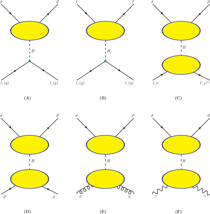
Figure 6: Classification of all the applications of the Higgs penguins. The vertex-dot indicates that the coupling is proportional to $\tan\beta$ for the weak isospin $(-1/2)$ quarks $q=d,s,b$ and leptons $l=e,\mu,\tau$. It is suppressed by $\cot\beta$ otherwise. The down quark Higgs penguin (blob with $d,d^{\prime}$ quarks) grows with two powers of $\tan\beta$ in the MSSM.

The Higgs penguin applications can be classified into the six categories depicted in Fig.(6):

• Quark single Higgs penguin decaying into a pair of leptons (l) or quarks (q) of the same family [Fig.6(A)]. This category includes the master application $B\to l\>l$ [37] that we have already discussed in the previous section. It leads also to contributions to the semileptonic B-decays $B\to X\>l\>l$ [19, 39, 57] and $K\to l\>l$. Forward-backward asymmetries in $B\to X\tau\tau$, $B\to\pi\>l\>l$ and $K\to\pi\>l\>l$ influenced by the Higgs penguin have been studied in [58], [59] and [60], respectively, and the lepton polarization asymmetry in $B\to l\>l$ or $K\to l\>l$ decays has been studied in [61] and [62], respectively. The decay into a quark pair $d^{\prime}\to d\>q\>q$ leads to a number of processes like $K\to\pi\pi$ [30], $B\to\pi\pi,B\to\phi K_{S},B\to J/\Psi\>K,B\to K\>\pi$ etc. In the MSSM, the amplitude grows like $\tan^{3}\beta$ if $q=d,s$ (or $l=e,\mu,\tau$), or with $\tan\beta$ if $q=u,c$. We have seen already that the Higgs penguin is in general complex [see for example, Eqs.(2.1,2.5)]. As a consequence, one can construct important CP-observables like, for example, the leptonic CP-asymmetry [63, 22, 30].

• Lepton Flavour Violating (LFV) single Higgs penguin decaying into pair of leptons (l) or quarks (q) [Fig.6(B)]. The LFV Higgs penguin has been calculated in the SM in Ref.[64]. In the MSSM, the method for calculating the Higgs penguin, presented in Ref.[30] and summarized here, may be easily extended to consistently account for charged-lepton flavour violating effective Lagrangian. The $\tau$-decays into three leptons $\tau\to(e,\mu)\>l\>l$ [65], or $\tau$-decays into a lepton and a pair of quarks $\tau\to(e,\mu)\>q\>q$, like $\tau\to\mu\eta$, belong to this category. The amplitude of these decays are neutrino mass generation mechanism dependent. For example, in the see-saw MSSM, $\tau\to 3l$ decays [66, 67, 68] are enhanced by three powers of $\tan\beta$ with the same happening in the $\tau\to lqq$ decays [69], or $\mu q\to eq$ amplitude ($\mu-e$ conversion in the nuclei) recently studied in [70]. On the contrary, decays with $\tau\to luu$ grow with only one power of $\tan\beta$.

• Quark-Lepton Flavour violating double Higgs penguin [Fig.6(C)]. This is nothing else than the combination of the cases (A) and (B). The processes $B\to l\>l^{\prime}$ [67], $B\to X\>l\>l^{\prime}$ and $\tau\to(e,\mu)\>K$, etc [71] belong to this category. They start formally at the two-loop level and they grow with four powers of $\tan\beta$. It is very interesting to notice that the double penguin (C) leads to invisible (at the detector) B-meson decays if the final particle state is a pair of neutrinos ($\nu$) of different flavour. This would be a unique signature at B-factories; we believe that it should be further studied from the theoretical point of view and searched for experimentally.

• Quark double Higgs penguin [Fig.6(D)]. Such processes lead to contributions to $B-\bar{B}$ or $K-\bar{K}$ mixing, and in the MSSM dominate over all other contributions for large $\tan\beta$. Although there is no similar analysis in the SM, following our discussion above, one expects that the diagram (D) is suppressed by a factor $(m_{b}/M_{W})^{4}$. In the MSSM, the dominant contribution to the $B_{s,d}-\bar{B}_{s,d}$ mixing is proportional to $m_{b}m_{s,d}\tan^{4}\beta/M_{H_{3}}^{2}$ [72, 30, 31], and to the $K-\bar{K}$ mixing proportional to $m_{d}m_{s,d}\tan^{4}\beta/M_{H_{3}}^{2}$ [30]. In addition, a complex double penguin leads to corrections on the CKM angle-$\beta$ originated from soft supersymmetry breaking complex parameters [30].

• Quark-Gluon double Higgs penguin [Fig.6(E)]. This is another class which is a combination of two penguins: the triangle Higgs-Gluon one (effective Lagrangian in the SM and in the MSSM can be found in [73]) and the Quark Higgs penguin reviewed here. They contribute to decays $B\to(X)\>g\>g$ and they scale at most like three powers of $\tan\beta$. No study of this Higgs mediated process exists so far in the literature.

• Quark-Photon double Higgs penguin [Fig.6(F)]. A combination with the photon triangle Higgs vertex - the main Higgs decay mode search at the LHC [73]. It leads to processes like $B\to(X)\gamma\gamma$ and scales at most like $\tan^{3}\beta$ when bottom quarks run in the photon triangle. No study for this amplitude exists in the literature.

All the above applications should be correlated with each other if they dominate in the corresponding processes. One example is the correlation between ${\cal B}(B_{s}\rightarrow\mu^{+}\mu^{-})$ and $B_{s}-\bar{B}_{s}$ mass difference, $\Delta M_{s}$, found in [72]. This correlation is valid in a specific scenario of squark mixing and is lost in a general case [30, 31]. Correlations among the full set of observables in Fig.6 would be an interesting probe of the MSSM squark flavour structure. As we can see, there is still a lot of work to be done along that direction.

4 Epilogue

In this brief review, we discussed the effective Lagrangian of the Higgs penguin both in the SM and in the MSSM, which are presented in Eqs. (2.1) and (2.5), respectively. The SM Higgs penguin exhibits a non-decoupling behaviour proportional to ${\bf{V}}^{\dagger}\>({\bf\hat{M}_{u}}^{2}/M_{W}^{2})\>{\bf{V}}$, but it is suppressed relative to the Z-penguin by a factor of $\sim m_{d}/M_{W}$. The MSSM Higgs penguin exhibits also a non-decoupling behavior but is further enhanced by two powers of $\tan\beta$, and dominates over the Z-penguin if $\tan\beta$ is large. We have in addition presented the applications of the Higgs penguin in B-meson, K-meson and $\tau$-lepton physics. The master application is the decay $\bar{B}_{q}\rightarrow l^{+}l^{-}$ . In the SM, the Higgs penguin contributes negligibly to ${\cal B}(B_{q}\rightarrow l^{+}l^{-})$ if the LEP experimental bound for the Higgs boson mass is taken into account. On the other hand in the MSSM, it is enhanced by three orders of magnitude mainly due to the $\tan\beta$ enhancement shown in Eq.(2.2.2). The B-decay mode $B_{s,d}\rightarrow\mu^{+}\mu^{-}$ is currently under high search priority at Tevatron and B-factories. As we explained in section 3.1.1 one of the most interesting aspects is the fact that a possible evidence for $B_{s}\rightarrow\mu^{+}\mu^{-}$ can probe the Higgs sector of the MSSM. Finally, we unfolded an exhaustive list of applications in Section 3.2, some of which are novel and not thoroughly studied even in the SM. We strongly believe that the Higgs penguin amplitudes deserve further theoretical and experimental investigation as their processes may soon leave their footprints at Hadron colliders and B-factories.

Acknowledgements: I would like to thank A. Buras, P. Chankowski, F. Krüger, A. Pilaftsis, K. Tamvakis for useful discussions and comments. Many thanks to P. Kanti for proofreading the manuscript. I would also like to thank the CERN Theory Division for the hospitality and financial support. I also acknowledge support by the German Bundesministerium für Bildung und Forschung under the contract 05HT1WOA3 and the ‘Deutsche Forschungsgemeinschaft’ DFG Project Bu. 706/1-2.

References

- [1] S. L. Glashow and S. Weinberg, Phys. Rev. D 15, 1958 (1977).
- [2] K. Hagiwara et al., Phys. Rev. D66, 010001 (2002)
- [3] T. Banks, Nucl. Phys. B 303 (1988) 172; E. Ma, Phys. Rev. D 39 (1989) 1922; R. Hempfling, Phys. Rev. D 49 (1994) 6168; L. J. Hall, R. Rattazzi and U. Sarid, Phys. Rev. D 50 (1994) 7048 [arXiv:hep-ph/9306309]; T. Blazek, S. Raby and S. Pokorski, Phys. Rev. D 52 (1995) 4151 [arXiv:hep-ph/9504364]; M. Carena, M. Olechowski, S. Pokorski and C. E. Wagner, Nucl. Phys. B 426 (1994) 269 [arXiv:hep-ph/9402253]; F. Borzumati, G. R. Farrar, N. Polonsky and S. Thomas, Nucl. Phys. B 555 (1999) 53 [arXiv:hep-ph/9902443].
- [4] R. S. Willey and H. L. Yu, Phys. Rev. D 26, 3086 (1982).
- [5] B. Grzadkowski and P. Krawczyk, Z. Phys. C 18 (1983) 43.
- [6] S. L. Glashow, J. Iliopoulos and L. Maiani, Phys. Rev. D 2 (1970) 1285.
- [7] F. J. Botella and C. S. Lim, Phys. Rev. Lett. 56, 1651 (1986); F. J. Botella and C. S. Lim, Phys. Rev. D 34, 301 (1986).
- [8] R. S. Chivukula and A. V. Manohar, Phys. Lett. B 207, 86 (1988) [Erratum-ibid. B 217, 568 (1989)].
- [9] B. Grinstein, L. J. Hall and L. Randall, Phys. Lett. B 211, 363 (1988).
- [10] G. Eilam and A. Soni, Phys. Lett. B 215, 171 (1988).
- [11] The full calculation of the Higgs penguin in the SM without restricting to zero external particle momenta has been presented in P. Krawczyk, Z. Phys. C 44, 509 (1989) and in B. Haeri, A. Soni and G. Eilam, Phys. Rev. D 41 (1990) 875.
- [12] A. A. Johansen, V. A. Khoze and N. G. Uraltsev, Sov. J. Nucl. Phys. 49, 727 (1989) [Yad. Fiz. 49, 1174 (1989)].
- [13] J. G. Korner, N. Nasrallah and K. Schilcher, Phys. Rev. D 41, 888 (1990).
- [14] R. Ferrari, A. Le Yaouanc, L. Oliver and J. C. Raynal, Phys. Rev. D 52, 3036 (1995).
- [15] T. Inami and C. S. Lim, Prog. Theor. Phys. 65 (1981) 297 [Erratum-ibid. 65 (1981) 1772]. See also p.25-28 in A. J. Buras, arXiv:hep-ph/9806471.
- [16] S. R. Choudhury and N. Gaur, Phys. Lett. B 451 (1999) 86 [arXiv:hep-ph/9810307].
- [17] C. S. Huang, W. Liao, Q. S. Yan and S. H. Zhu, Phys. Rev. D 63 (2001) 114021 [Erratum-ibid. D 64 (2001) 059902] [arXiv:hep-ph/0006250].
- [18] P. H. Chankowski and L. Slawianowska, Phys. Rev. D 63 (2001) 054012 [arXiv:hep-ph/0008046].
- [19] C. Bobeth, T. Ewerth, F. Krüger and J. Urban, Phys. Rev. D 64 (2001) 074014 [arXiv:hep-ph/0104284].
- [20] C. Bobeth, T. Ewerth, F. Krüger and J. Urban, Phys. Rev. D 66 (2002) 074021 [arXiv:hep-ph/0204225].
- [21] A. Dedes, H. K. Dreiner and U. Nierste, Phys. Rev. Lett. 87 (2001) 251804 [arXiv:hep-ph/0108037].
- [22] T. Ibrahim and P. Nath, Phys. Rev. D 67 (2003) 016005 [arXiv:hep-ph/0208142].
- [23] A. M. Curiel, M. J. Herrero and D. Temes, Phys. Rev. D 67 (2003) 075008 [arXiv:hep-ph/0210335].
- [24] W. Skiba and J. Kalinowski, Nucl. Phys. B 404 (1993) 3.
- [25] H. E. Logan and U. Nierste, Nucl. Phys. B 586, 39 (2000) [arXiv:hep-ph/0004139].
- [26] K. S. Babu and C. F. Kolda, Phys. Rev. Lett. 84 (2000) 228 [arXiv:hep-ph/9909476].
- [27] G. Isidori and A. Retico, JHEP 0111 (2001) 001 [arXiv:hep-ph/0110121]; JHEP 0209 (2002) 063 [arXiv:hep-ph/0208159].
- [28] J. K. Mizukoshi, X. Tata and Y. Wang, Phys. Rev. D 66 (2002) 115003 [arXiv:hep-ph/0208078].
- [29] G. D’Ambrosio, G. F. Giudice, G. Isidori and A. Strumia, Nucl. Phys. B 645 (2002) 155 [arXiv:hep-ph/0207036].
- [30] A. Dedes and A. Pilaftsis, Phys. Rev. D 67 (2003) 015012 [arXiv:hep-ph/0209306]. We follow the notation and conventions of this article.
- [31] A. J. Buras, P. H. Chankowski, J. Rosiek and L. Slawianowska, Nucl. Phys. B 659 (2003) 3 [arXiv:hep-ph/0210145].
- [32] D. A. Demir, arXiv:hep-ph/0303249.
- [33] A. Pilaftsis, Phys. Rev. D58 (1998) 096010; Phys. Lett. B435 (1998) 88; A. Pilaftsis and C.E.M. Wagner, Nucl. Phys. B553 (1999) 3; D.A. Demir, Phys. Rev. D60 (1999) 055006; S.Y. Choi, M. Drees and J.S. Lee, Phys. Lett. B481 (2000) 57; G.L. Kane and L.-T. Wang, Phys. Lett. B488 (2000) 383; T. Ibrahim and P. Nath, Phys. Rev. D63 (2001) 035009;
- [34] See, for example, J. R. Ellis and D. V. Nanopoulos, Phys. Lett. B 110, 44 (1982); J.F. Donoghue, H.P. Nilles and D. Wyler, Phys. Lett. B128 (1983) 55; J.M. Gerard, W. Grimus, A. Raychaudhuri and G. Zoupanos, Phys. Lett. B140 (1984) 349.
- [35] See p.201-204 in S. Weinberg, “The Quantum Theory Of Fields. Vol. 3: Supersymmetry,”, Cambridge,UK: Univ. Pr. (2000) 419 p.
- [36] The leading order calculation of the Z-penguins and the box contributions to the decay in the SM was carried out by T. Inami and C. S. Lim, in Ref.[15]. NLO QCD corrections were considered in G. Buchalla and A. J. Buras, Nucl. Phys. B 400 (1993) 225 and later in M. Misiak and J. Urban, Phys. Lett. B 451 (1999) 161 [arXiv:hep-ph/9901278]. The Higgs penguin contribution to was very popular in the eighties because there was almost no bound on the Higgs mass. Thus the Higgs searches were actually carried out by B-, or K-meson decays. Relevant references are [4, 5, 8, 9, 10] and J. F. Gunion, H. E. Haber, G. L. Kane and S. Dawson, “The Higgs Hunter’s Guide”, SCIPP-89/13.
- [37] There is a vast number of articles calculating the Higgs penguin contributions to the in the 2HDM [24, 25, 17, 19, 39] and general MSSM [16, 26, 17, 18, 19, 20, 27, 29, 30, 31, 39]. mSUGRA and mGMSB/mAMSB results for the appeared in [21, 41, 28, 38, 22, 42] and in [42], respectively. SO(10) GUT predictions for the have been discussed in [43, 21, 44, 45]. Gluino loop NLO corrections to have been calculated in [46].
- [38] A. Dedes, H. K. Dreiner, U. Nierste and P. Richardson, arXiv:hep-ph/0207026.
- [39] C. S. Huang and X. H. Wu, Nucl. Phys. B 657, 304 (2003) [arXiv:hep-ph/0212220].
- [40] One can further reduce the uncertainties for the SM expectation in the by using the experimental value of . With the same method one can reduce uncertainties in the SM prediction of by using when of course this is experimentally known. This method has been proposed in A. J. Buras, Phys. Lett. B 566 (2003) 115 [arXiv:hep-ph/0303060].
- [41] R. Arnowitt, B. Dutta, T. Kamon and M. Tanaka, Phys. Lett. B 538 (2002) 121 [arXiv:hep-ph/0203069].
- [42] S. Baek, P. Ko and W. Y. Song, Phys. Rev. Lett. 89 (2002) 271801 [arXiv:hep-ph/0205259]; JHEP 0303 (2003) 054 [arXiv:hep-ph/0208112].
- [43] C. Hamzaoui and M. Pospelov, Phys. Rev. D 60 (1999) 036003 [arXiv:hep-ph/9901363].
- [44] R. Dermisek, S. Raby, L. Roszkowski and R. Ruiz De Austri, JHEP 0304 (2003) 037 [arXiv:hep-ph/0304101].
- [45] T. Blazek, S. F. King and J. K. Parry, arXiv:hep-ph/0308068.
- [46] C. Bobeth, A. J. Buras, F. Krüger and J. Urban, Nucl. Phys. B 630, 87 (2002) [arXiv:hep-ph/0112305].
- [47] If the R-parity symmetry is replaced by a Baryon parity symmetry in the MSSM, then can appear at tree level. See for instance, J. H. Jang, J. K. Kim and J. S. Lee, Phys. Rev. D 55 (1997) 7296 [arXiv:hep-ph/9701283]; A. G. Akeroyd and S. Recksiegel, arXiv:hep-ph/0209252; D. Guetta, J. M. Mira and E. Nardi, Phys. Rev. D 59 (1999) 034019 [arXiv:hep-ph/9806359]. For the calculation of the in extended technicolor models, see: L. Randall and R. Sundrum, Phys. Lett. B 312 (1993) 148 [arXiv:hep-ph/9305289]; Z. h. Xiong and J. M. Yang, Phys. Lett. B 546, 221 (2002) [arXiv:hep-ph/0208147]. For the calculation of the in models with extra dimensions, see: A. J. Buras, M. Spranger and A. Weiler, Nucl. Phys. B 660 (2003) 225 [arXiv:hep-ph/0212143]; P. Dey and G. Bhattacharyya, arXiv:hep-ph/0309110.
- [48] W. Adam et al. [DELPHI Collaboration], Z. Phys. C 72 (1996) 207.
- [49] F. Azfar, arXiv:hep-ex/0309005, presented at “XXIII Physics in Collision”, Zeuthen, Germany, 26-28 June 2003. This is a preliminary new Run II bound for the channel . The 95% CL bound reads . It is by a factor of two improved bound relative to the “old” CDF Run I bound reported in F. Abe et al. [CDF Collaboration], Phys. Rev. D 57 (1998) 3811. The improved CDF bound makes the mode the most preferred one in probing the MSSM parameter space among all .
- [50] This is a byproduct bound from LEP searches on the mode and was pointed out in Y. Grossman, Z. Ligeti and E. Nardi, Phys. Rev. D 55 (1997) 2768 [arXiv:hep-ph/9607473]. There is no experimental analysis for the channel . We would like to encourage our experimental colleagues to search for this, motivated by the fact that in the supersymmetric extensions of the Standard model this mode is enhanced by three orders of magnitude relative to its SM prediction in Table 1.
- [51] M.-C. Chang, et al, [Belle Collaboration], KEK Preprint 2003-44, Belle Preprint 2003-12, arXiv:hep-ex/0309069. For BaBar results on rare leptonic B decays, see T. B. Moore, SLAC-PUB-9705, presented at 31st International Conference on High Energy Physics (ICHEP 2002), Amsterdam, The Netherlands, 24-31 Jul 2002; V. Halyo, arXiv:hep-ex/0207010.
- [52] The lattice values for are taken from C. W. Bernard, Nucl. Phys. Proc. Suppl. 94 (2001) 159 [arXiv:hep-lat/0011064]. They are consistent with those reported recently by D. Becirevic, at 2nd Workshop On The CKM Unitarity Triangle 5-9 Apr 2003.
- [53] K. Anikeev et al., arXiv:hep-ph/0201071.
- [54] T. Kamon [CDF Collaboration], arXiv:hep-ex/0301019.
- [55] P. Ball et al., arXiv:hep-ph/0003238.
- [56] J. S. Lee, A. Pilaftsis, M. Carena, S. Y. Choi, M. Drees, J. Ellis and C. E. Wagner, arXiv:hep-ph/0307377.
- [57] C. S. Huang and Q. S. Yan, Phys. Lett. B 442 (1998) 209 [arXiv:hep-ph/9803366]; C. S. Huang, W. Liao and Q. S. Yan, Phys. Rev. D 59 (1999) 011701 [arXiv:hep-ph/9803460]; Y. Wang and D. Atwood, arXiv:hep-ph/0304248. P. H. Chankowski and L. Slawianowska, arXiv:hep-ph/0308032. For a recent review on see, T. Hurth, arXiv:hep-ph/0212304.
- [58] A. S. Cornell and N. Gaur, arXiv:hep-ph/0308132.
- [59] S. R. Choudhury, A. S. Cornell, N. Gaur and G. C. Joshi, arXiv:hep-ph/0307276.
- [60] C. H. Chen, C. Q. Geng and I. L. Ho, Phys. Rev. D 67 (2003) 074029 [arXiv:hep-ph/0302207].
- [61] L. T. Handoko, C. S. Kim and T. Yoshikawa, Phys. Rev. D 65 (2002) 077506 [arXiv:hep-ph/0112149].
- [62] P. Herczeg, Phys. Rev. D 27, 1512 (1983). S. R. Choudhury, N. Gaur and A. Gupta, Phys. Lett. B 482 (2000) 383 [arXiv:hep-ph/9909258].
- [63] C.S. Huang and W. Liao, Phys. Lett. B525 (2002) 107; Phys. Lett. B538 (2002) 301; P.H. Chankowski and L. Slawianowska, Acta Phys. Polon. B32 (2001) 1895. Y. B. Dai, C. S. Huang, J. T. Li and W. J. Li, Phys. Rev. D 67, 096007 (2003) [arXiv:hep-ph/0301082].
- [64] A. Pilaftsis, Phys. Lett. B 285 (1992) 68.
- [65] For a recent experimental status of and LFV decays, see Y. Yusa, H. Hayashii, T. Nagamine and A. Yamaguchi [BELLE Collaboration], eConf C0209101 (2002) TU13 [arXiv:hep-ex/0211017].
- [66] K. S. Babu and C. Kolda, Phys. Rev. Lett. 89 (2002) 241802 [arXiv:hep-ph/0206310].
- [67] A. Dedes, J. R. Ellis and M. Raidal, Phys. Lett. B 549 (2002) 159 [arXiv:hep-ph/0209207].
- [68] A. Brignole and A. Rossi, Phys. Lett. B 566 (2003) 217 [arXiv:hep-ph/0304081].
- [69] M. Sher, Phys. Rev. D 66 (2002) 057301 [arXiv:hep-ph/0207136].
- [70] R. Kitano, M. Koike, S. Komine and Y. Okada, arXiv:hep-ph/0308021.
- [71] D. Black, T. Han, H. J. He and M. Sher, Phys. Rev. D 66 (2002) 053002 [arXiv:hep-ph/0206056].
- [72] A. J. Buras, P. H. Chankowski, J. Rosiek and L. Slawianowska, Phys. Lett. B 546 (2002) 96 [arXiv:hep-ph/0207241].
- [73] M. Spira, Fortsch. Phys. 46 (1998) 203 [arXiv:hep-ph/9705337].