HIP-2003-46/TH

ROME1-1360/2003

Violation of Angular Momentum Selection Rules
in Quantum Gravity

 

Abstract

A simple consequence of the angular momentum conservation in quantum field theories is that the interference of $s$-channel amplitudes exchanging particles with different spin $J$ vanishes after complete angular integration. We show that, while this rule holds in scattering processes mediated by a massive graviton in Quantum Gravity, a massless graviton $s$-channel exchange breaks orthogonality when considering its interference with a scalar-particle $s$-channel exchange, whenever all the external states are massive. As a consequence, we find that, in the Einstein theory, unitarity implies that angular momentum is not conserved at quantum level in the graviton coupling to massive matter fields. This result can be interpreted as a new anomaly, revealing unknown aspects of the well-known van Dam - Veltman - Zakharov discontinuity.

 

1 Introduction

It is well known that, when considering a massive spin-2 gravitational field in quantum gravity, the limit of vanishing graviton mass is distinct from the prediction of the massless-graviton Einstein theory. In [1], [2], van Dam, Veltman, and Zakharov (vDVZ) stressed this problem considering the leading tree-level approximation to the graviton exchange between matter sources, for a massive graviton coupled to matter as $h^{\mu\nu}T_{\mu\nu}$ (with $T_{\mu\nu}$ the conserved energy-momentum tensor and $h^{\mu\nu}$ the graviton field). The vDVZ discontinuity is shown to arise from the fact that a massive spin-2 tensor field has five polarization degrees of freedom, while a massless spin-2 graviton has simply two. In the massless limit, the massive graviton decomposes into three massless fields with spin-2, spin-1 and spin-0, respectively. The spin-1 vector field has a derivative coupling to the conserved energy-momentum tensor, and its contribution to the one graviton exchange amplitude vanishes. On the other hand, the spin-0 scalar field is coupled to the trace of the energy-momentum tensor and contributes in general to the scattering amplitude. This scalar component does not decouple even in the massless graviton limit. This gives rise to a discontinuity in the predictions of the massive and massless theory in the lowest tree-level approximation. As a consequence, in the massive theory (even in the limit of small masses) the light bending by the Sun and the precession of the Mercury perihelion differ by numerical factors from the predictions of the Einstein theory.

Many papers have elaborated on the possibility to fix this apparent inconsistency of the massive theory, in different directions [3]-[7]. For instance, in [3] it is claimed that, if the light bending by the sun is computed by solving the exact space-time metric equation in the presence of a small graviton mass, no discontinuity arises in the limit of small graviton mass. In fact, the discontinuity could be connected to the use of perturbation theory for the metric fluctuations around the flat space-time. More recently, it has been shown that there is not any vDVZ discontinuity in the De Sitter space [4] (or in the Anti De Sitter space [5]), where the massless graviton limit is smooth (see also [6], [7] for other solutions).

Here, we present a different class of problems connected to the vDVZ discontinuity. In particular, we stress the fact that there are cases where, while the massive theory is well-behaved, a massless graviton gives rise to inconsistencies. In particular, we show that the massless graviton propagator in the Einstein theory breaks angular momentum selection rules.

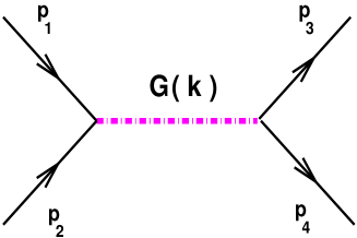
Figure 1: Scattering $p_{1}\,p_{2}\to p_{3}\,p_{4}$ in the $s$-channel with a graviton exchange.

Let us consider the tree-level amplitude for the graviton exchange in the $s$-channel between two on-shell matter fields (Fig. 1). The two on-shell matter fields enter into the amplitude through the conserved (at the zeroth order in $h_{\mu\nu}$) symmetric energy-momentum tensors $T_{\mu\nu}$ and $T^{\prime}_{\alpha\beta}$, respectively.

For a massive spin-2 field of momentum $k$ and mass $m_{G}$, one has five independent polarization tensors $\epsilon_{\mu\nu}(k,\sigma)$, where the index $\sigma$ runs over the polarization states. Summing over all polarizations, one gets [1]

$$\sum_{\sigma=1}^{5}\epsilon_{\mu\nu}(k,\sigma)\,\epsilon_{\alpha\beta}(k,\sigma)=P^{m}_{\mu\nu\alpha\beta}(k)$$ (1)

with

$$P^{m}_{\mu\nu\alpha\beta}(k) = \frac{1}{2}\left(\eta_{\mu\alpha}\eta_{\nu\beta}+\eta_{\mu\beta}\eta_{\nu\alpha}-\eta_{\mu\nu}\eta_{\alpha\beta}\right)$$ (2)

$$- \frac{1}{2\,m_{G}^{2}}\left(\eta_{\mu\alpha}k_{\mu}k_{\beta}+\eta_{\nu\beta}k_{\mu}k_{\alpha}+\eta_{\mu\beta}k_{\nu}k_{\beta}+\eta_{\nu\alpha}k_{\mu}k_{\beta}\right)$$

$$+ \frac{1}{6}\left(\eta_{\mu\nu}+\frac{2}{m_{G}^{2}}k_{\mu}k_{\nu}\right)\left(\eta_{\alpha\beta}+\frac{2}{m_{G}^{2}}k_{\alpha}k_{\beta}\right).$$

The projector $P^{m}_{\mu\nu\alpha\beta}$ is symmetric and traceless in both $(\mu,\nu)$ and $(\alpha,\beta)$ indices, and satisfies the transversality conditions $k^{\mu}P^{m}_{\mu\nu\alpha\beta}=k^{\alpha}P^{m}_{\mu\nu\alpha\beta}=0$.

For a massless graviton, one has just two transverse polarization states $(\sigma=1,2)$, that correspond to the helicity values $\lambda=\pm 2$. The sum over polarizations is then [1]

$$\sum_{\sigma=1}^{2}\epsilon_{\mu\nu}(k,\sigma)\,\epsilon_{\alpha\beta}(k,\sigma)=P_{\mu\nu\alpha\beta}(k)=\frac{1}{2}\left(\eta_{\mu\alpha}\eta_{\nu\beta}+\eta_{\mu\beta}\eta_{\nu\alpha}-\eta_{\mu\nu}\eta_{\alpha\beta}\right)+\dots\;,$$ (3)

where dots stand for terms containing at least one graviton momentum.

In the unitary gauge, the corresponding massive and massless graviton propagators are proportional to the projectors $P^{m}_{\mu\nu\alpha\beta}$ and $P_{\mu\nu\alpha\beta}$, respectively [1]. However, terms proportional to the graviton momentum in Eqs.(2) and (3) vanish when contracted with $T_{\mu\nu}$ in the on-shell matrix elements, due to the conservation of the energy-momentum tensor. For this reason, the tree-level diagram with one graviton exchange in Fig.1 is gauge invariant, and the effective massive and massless graviton propagators become [1]

$$G^{m}_{\mu\nu\alpha\beta}(k) = i\,\;\frac{\frac{1}{2}\eta_{\mu\alpha}\eta_{\nu\beta}+\frac{1}{2}\eta_{\mu\beta}\eta_{\nu\alpha}-\frac{1}{3}\eta_{\mu\nu}\eta_{\alpha\beta}}{k^{2}-m^{2}_{G}+i\epsilon}$$ (4)

$$G_{\mu\nu\alpha\beta}(k) = i\,\;\frac{\frac{1}{2}\eta_{\mu\alpha}\eta_{\nu\beta}+\frac{1}{2}\eta_{\mu\beta}\eta_{\nu\alpha}-\frac{1}{2}\eta_{\mu\nu}\eta_{\alpha\beta}}{k^{2}+i\epsilon}.$$ (5)

As shown in [1], unitarity fixes uniquely the coefficients of the Minkowski metric products in Eqs.(4) and (5).

The corresponding on-shell $s$-channel matrix elements will be then, up to some coupling constant,

$${\cal A}^{m}\sim T^{\mu\nu}\;G^{m}_{\mu\nu\alpha\beta}(k)\;T^{\prime\,\alpha\beta}$$ (6)

and

$${\cal A}\sim T^{\mu\nu}\;G_{\mu\nu\alpha\beta}(k)\;T^{\prime\,\alpha\beta}$$ (7)

In the limit $m_{G}\to 0$, Eqs. (6) and (7) only differ by the coefficients of the $\eta_{\mu\nu}\eta_{\alpha\beta}$ term in Eqs.(4) and (5). When contracted with the energy-momentum tensors, the latter give terms proportional to the traces $T_{\mu}^{\mu}$ and $T^{\prime\alpha}_{\alpha}$, that are nonvanishing for massive external fields. From this difference, the vDVZ discontinuity arises [1].

Note that the terms in the amplitudes corresponding to the $\eta_{\mu\nu}\eta_{\alpha\beta}$ terms in the graviton propagators can be interpreted as a scalar field exchange amplitude .

Let us consider now the interference of the $s$-channel amplitudes exchanging particles of different spin $J$ (Fig. 2).

$${\cal I}(i,j)\sim\;{\cal A}^{\star}(J=i)\;\times\;{\cal A}(J=j)\,+h.c.\,\;\;\;\;\;\;(j\neq i)\,$$ (8)

A simple consequence of angular momentum conservation is that, after complete angular integration on the final state, this quantity must vanish, that is

$$\int d\cos\theta\;d\varphi\;\;{\cal I}(i,j)=0\;\;\;\;\;\;(j\neq i)\,,$$ (9)

where $\theta$ is the scattering angle and $\varphi$ is the azimuthal angle in the center of mass frame. For instance, it is straightforward to verify this in gauge theories, looking at the interference of a vector boson exchange with a scalar (Higgs boson) particle exchange.

One then expects the same is true for the interference of the $J=2$ and $J=0$ amplitudes. On the other hand, we have seen above that (in the small $m_{G}$ limit) the massive and massless graviton propagator effectively differs by a scalar field exchange, when the external fields are massive. This extra scalar field component, when interfering with a spin-0 exchange amplitude, will give a nonvanishing contribution to $\int d\cos\theta\;d\varphi\;{\cal I}(2,0)\;$. This implies that the orthogonality condition in Eq. (9) for the interference ${\cal I}(2,0)$ can be verified either for the massive graviton exchange or for the massless graviton exchange, but can NOT hold in both cases at the same time.

We checked the above statement by an explicit calculation. The result is that the orthogonality condition in Eq.(9) holds for the massive graviton exchange, but not in the Einstein theory !
For a massless graviton and massive external states, one finds

$$\int d\cos\theta\;d\varphi\;\;{\cal I}(2,0)\;\neq\;0.$$ (10)

In the following, we illustrate this result, by giving the explicit expressions of the above discontinuity for the scattering of different external states. We will also extend the discussion to the interferences of the graviton graphs with vector-boson exchange diagrams in the $s$ channel. As a theoretical framework, we assume the Standard Model minimally coupled to gravity (e.g., as in [8]).

2 The Graviton-Scalar Interference

In the following, we will discuss the interference of the on-shell tree-level scattering amplitudes in the $s$-channel mediated by a graviton ($J=2$) with either a scalar particle exchange ($J=0$) or a vector particle exchange ($J=1$), as in Fig. 2. We consider initial and final states containing either massive fermions or massive vector bosons.

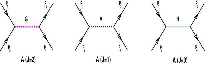
Figure 2: Scattering $p_{1}\,p_{2}\to p_{3}\,p_{4}$ in the $s$-channel with different spin-$J$ particle exchange.

For each $s$ scattering channel,

$$a+\bar{a}\to b+\bar{b},$$ (11)

it is convenient to introduce the dimensionless quantities $\;{\cal I}^{m}_{a,b}(2,j)\;$ and $\;{\cal I}_{a,b}(2,j)\;$ connected to the interferences of the massive and massless graviton amplitudes, ${\cal A}^{m}_{a,b}(J=2)$ and ${\cal A}_{a,b}(J=2)$, respectively, and the amplitude mediated by a particle of spin $j\;$, $\;{\cal A}_{a,b}(J=j)$, with $j=0,1$.
The crucial point is that the two amplitudes ${\cal A}^{m}_{a,b}(J=2)$ and ${\cal A}_{a,b}(J=2)$ depend on the two different (massive or massless) graviton propagators in Eqs.(4) and (5), respectively.
By setting $r_{j}=m_{j}^{2}/s$ [with $m_{j}=m_{0}\;(m_{1})$ for the exchange of a scalar (vector) particle of mass $m_{0}\;(m_{1})$] and $r_{G}=m_{G}^{2}/s$, with $\sqrt{s}$ the c.m. scattering energy, we define

$${\cal I}^{m}_{a,b}(2,j) \equiv \frac{M_{P}^{2}}{s}(1-r_{j})(1-r_{G})\sum_{\rm pol}{\cal A}_{a,b}^{\star}(J=j)\times{\cal A}_{a,b}^{m}(J=2)+h.c.\;,$$ (12)

$${\cal I}_{a,b}(2,j) \equiv \frac{M_{P}^{2}}{s}(1-r_{j})\sum_{\rm pol}{\cal A}_{a,b}^{\star}(J=j)\times{\cal A}_{a,b}(J=2)+h.c.\;,$$ (13)

where $M_{P}$ is the reduced Planck mass (see Appendix I), and a sum over all the external particles polarization states is performed.
Note that, by definition, the quantities ${\cal I}^{m}_{a,b}(2,j)$ and ${\cal I}_{a,b}(2,j)$ depend neither on the masses of particles exchanged in the propagators nor on the Plank mass.
Since we are interested into the discontinuity in the massive and massless graviton interferences, it is useful to define also the quantity $\Delta_{a,b}(2,j)$,

$$\Delta_{a,b}(2,j)\;\equiv\;\;{\cal I}_{a,b}(2,j)-{\cal I}^{m}_{a,b}(2,j)\;,$$ (14)

that gives the excess in the Einstein interference ${\cal I}_{a,b}(2,j)$ with respect to the massive graviton interference ${\cal I}^{m}_{a,b}(2,j)$ [when $j=0$, $\Delta_{a,b}(2,j)$ will be directly connected to the vDVZ discontinuity].

Following the discussion in the previous section, we now concentrate on the graviton interference with a scalar particle, and express all our results in terms of the massive graviton interference ${\cal I}^{m}_{a,b}(2,0)$ and the discontinuity $\Delta_{a,b}(2,0)\;$. In the $J=0$ propagator, we assume as a scalar particle a Higgs boson, coupled as in the standard model (see Appendix I ). The following external states are considered :
a) the scattering of two electrons into a pair of fermions $f$, with $f\neq e$;
b) the scattering of two electrons into a pair of gauge vector bosons $W$ ;
c) the scattering of two $W$’s into a pair of gauge vector bosons $W^{\prime}$, with $W^{\prime}\neq W$.

In the following, $r_{i}=m_{i}^{2}/s$, $\;\beta_{i}=\sqrt{1-4r_{i}}\;\;$ ($i=e,f,W,W^{\prime}$), and $\lambda_{e}$ $(\lambda_{f})$ is the $e$ $(f)$ Yukawa coupling. The angle $\theta$ is the scattering angle of a final particle with given electric charge with respect to the initial particle of same charge, in the c.m. system.
Following the Feynman rules in Appendix I, one then gets

• ${\bf e^{+}e^{-}\to f\bar{f}}$

  $${\cal I}^{m}_{e,f}(2,0) = -\frac{8}{3}\lambda_{e}\lambda_{f}\beta_{e}^{2}\beta_{f}^{2}\,\sqrt{r_{e}r_{f}}\left(1-3\cos^{2}{\theta}\right)$$ (15)

  and

  $$\Delta_{e,f}(2,0)=-\frac{4}{3}\lambda_{e}\lambda_{f}\beta_{e}^{2}\beta_{f}^{2}\,\sqrt{r_{e}r_{f}}$$ (16)

• ${\bf e^{+}e^{-}\to W^{+}W^{-}}$

  $${\cal I}^{m}_{e,W}(2,0) = -\frac{1}{3}\lambda_{e}g_{W}\sqrt{\frac{r_{e}}{r_{W}}}\beta_{e}^{2}\beta_{W}^{2}\,\left(1+6r_{W}\right)\left(1-3\cos^{2}{\theta}\right)$$ (17)

  and

  $$\Delta_{e,W}(2,0)=\frac{1}{12}\lambda_{e}g_{W}\sqrt{\frac{r_{e}}{r_{W}}}\beta_{e}^{2}\left(3+\beta_{W}^{2}\left(1-12r_{W}\right)\right)$$ (18)

• ${\bf W^{+}W^{-}\to W^{\prime+}W^{\prime-}}$

  $${\cal I}^{m}_{W,W^{\prime}}(2,0) = -\frac{1}{24}\frac{g_{W}g_{W^{\prime}}}{\sqrt{r_{W}r_{W^{\prime}}}}\beta_{W}^{2}\beta_{W^{\prime}}^{2}\left(1+6r_{W}\right)\left(1+6r_{W^{\prime}}\right)\,\left(1-3\cos^{2}{\theta}\right)\;\;$$ (19)

  and

  $$\Delta_{W,W^{\prime}}(2,0)=-\frac{1}{12}\frac{g_{W}g_{W^{\prime}}}{\sqrt{r_{W}r_{W^{\prime}}}}\beta_{W}^{2}\beta_{W^{\prime}}^{2}\left(\beta_{W}^{2}+12r_{W}^{2}\right)\,\left(\beta_{W^{\prime}}^{2}+12r_{W^{\prime}}^{2}\right).$$ (20)

Then, in each of the above channels, we have for the graviton-scalar interference in the Einstein theory

$${\cal I}_{a,b}(2,0)={\cal I}^{m}_{a,b}(2,0)+\Delta_{a,b}(2,0),$$ (21)

with a $\theta$ independent discontinuity $\Delta_{a,b}(2,0)$.

The angular integration $\int d\cos\theta$ of all the massive graviton interferences, ${\cal I}^{m}_{a,b}(2,0)$, has a vanishing results (respecting angular momentum selection rules). On the other hand, the angular integration of the massless graviton interference always gives rise to a nonnull results (for massive external states), that is

$$\int^{1}_{-1}d\cos\theta\;{\cal I}_{a,b}(2,0)=\int^{1}_{-1}d\cos\theta\;\Delta_{a,b}(2,0)=\;2\;\;\Delta_{a,b}(2,0)\neq 0\;,$$ (22)

that is connected to the vDVZ discontinuity.

Note that the results above do not depend on the gauge choice. For instance, in a covariant gauge, the gauge dependence affects the graviton propagators only through momentum dependent terms, that vanish after contraction with the energy-momentum tensors.

In Eqs.(15)-(18), the interferences are all vanishing in the massless fermion limit ($r_{e,f}\to 0$), due to fermion chirality. The $J=2$ amplitude conserves the chirality, while the opposite is true for the $J=0$ scalar channel. Then, in order to get a nonvanishing result for the interference, a chirality flip is needed in the initial/ final fermion states, giving rise to the fermion mass factor. In Eqs.(17)-(20), the singularity in the external gauge-boson mass ($1/\sqrt{r_{W}}$ and $1/\sqrt{r_{W}^{\prime}}$ terms) arises from the sum over the gauge bosons polarizations, since longitudinal modes do not decouple in the massless gauge boson limit .

From the results above, assuming angular momentum conservation at each interaction vertex, one could conclude that the Einstein graviton propagator behaves as if it was propagating a further scalar degree of freedom that is coupled to the masses of external states. However, this would be in contrast with unitarity and the conservation of the energy momentum tensor. Indeed, only the spin-2 transverse polarizations $\epsilon_{\mu\nu}(k,\sigma)$ with helicities $\lambda=\pm 2$ are effectively exchanged in the massless graviton propagator (see [1] for details). Then, in the Einstein theory, unitarity implies that angular momentum is not conserved at quantum level in the graviton coupling to massive matter fields, even if the total angular momentum is conserved in the scattering process.

We checked the results relative to the fermion-fermion scattering by computing the expansion in terms of spherical harmonics (i.e., the angular momentum eigenstates, ${\bf Y_{l}^{m}}(\theta,\varphi)$, defined in the Appendix I ) of the scattering amplitudes, for the four-fermion processes

$$e^{+}(p_{1},\nu_{1})\,+\,e^{-}(p_{2},\nu_{2})\,\to\,(J=0,1,2)\,\to\,\bar{f}(p_{3},\nu_{3})\,+\,f(p_{4},\nu_{4})$$ (23)

where a virtual particle of spin $J=0,1,2$ is exchanged in the $s$ channel, and $p_{i}$ and $\nu_{i}$ ($i=1,2,3,4$) stands for the external particles momenta and helicities, respectively. We will work in the c.m. frame, where the momenta $p_{i}$ can be cast in the following form

$$p_{1} = \frac{\sqrt{s}}{2}(1,0,0,\beta_{e}),~{}~{}~{}p_{2}=\frac{\sqrt{s}}{2}(1,0,0,-\beta_{e}),$$

$$p_{3} = \frac{\sqrt{s}}{2}(1,\beta_{f}\sin{\theta}\cos{\varphi},\beta_{f}\sin{\theta}\sin{\varphi},\beta_{f}\cos{\theta}),$$

$$p_{4} = \frac{\sqrt{s}}{2}(1,-\beta_{f}\sin{\theta}\cos{\varphi},-\beta_{f}\sin{\theta}\sin{\varphi},-\beta_{f}\cos{\theta})\,,$$ (24)

with $\varphi$ being the azimuthal angle.

In order to express the $J=0,1,2$ helicity amplitudes as a linear combination of the spherical harmonics ${\bf Y_{l}^{m}}(\theta,\varphi)$, it is convenient to use the solution of the Dirac equation for the particle ($U$) and antiparticle ($V$) bispinors in the momentum space [10]

$$U(p,\nu)=\left(\begin{array}[]{c}\sqrt{\epsilon+m}\,\,\omega_{\nu}(\underline{n})\\ \sqrt{\epsilon-m}\,\,\left(\underline{\sigma}\cdot\underline{n}\right)\omega_{\nu}(\underline{n})\end{array}\right)~{}~{}~{}~{}~{}V(p,-\nu)=\left(\begin{array}[]{c}\sqrt{\epsilon-m}\,\,\left(\underline{\sigma}\cdot\underline{n}\right)\omega_{\nu}(\underline{n})\\ \sqrt{\epsilon+m}\,\,\omega_{\nu}(\underline{n})\end{array}\right),$$ (29)

where the 2-component spinors $\omega_{\nu}(\underline{n})$ (with $\nu=\pm 1$) are the eigenstates of the helicity operator $\left(\underline{\sigma}\cdot\underline{n}\right)\omega_{\nu}(\underline{n})=\nu\,\omega_{\nu}(\underline{n})$, and $\;\sigma_{i}$ are the Pauli matrices. Here, $\underline{n}=\underline{p}/|\underline{p}|$, where $\underline{p}$ is the 3-momentum $\underline{p}=|\underline{p}|\left(\sin{\theta}\cos{\varphi},\sin{\theta}\sin{\varphi},\cos{\theta}\right)$, and $\epsilon$ is the corresponding energy. In polar coordinates, $\omega_{\nu}(\underline{n})$ can be expressed as

$$\omega_{+1}(\underline{n})=\left(\begin{array}[]{c}e^{-i\frac{\varphi}{2}}\,\cos{\frac{\theta}{2}}\\ e^{i\frac{\varphi}{2}}\,\sin{\frac{\theta}{2}}\end{array}\right)\,,~{}~{}~{}~{}~{}\omega_{-1}(\underline{n})=\left(\begin{array}[]{c}-e^{-i\frac{\varphi}{2}}\,\sin{\frac{\theta}{2}}\\ e^{i\frac{\varphi}{2}}\,\cos{\frac{\theta}{2}}\end{array}\right)\,.$$ (34)

After some straightforward algebra, the ${\cal A}(J=0,1,2)$ helicity amplitudes for the channels in Eq.(23) can be cast in the following form, as a function of the initial and final helicities ($\nu_{i}=\pm 1$) ,

$${\cal A}(J=0) = R_{0}\,\left\{\,\delta_{\nu_{1},\nu_{2}}\delta_{\nu_{3},\nu_{4}}\nu_{1}\nu_{3}\,{\bf Y_{0}^{0}}\,\right\}\;,$$ (35)

$${\cal A}(J=1) = R_{1}\,\left\{\,\delta_{\nu_{1},-\nu_{2}}\delta_{\nu_{3},-\nu_{4}}\left({\bf Y_{1}^{0}}+\sqrt{3}\,\nu_{1}\nu_{3}\,{\bf Y_{0}^{0}}\right)\right.$$ (36)

$$- \left.\delta_{\nu_{1},-\nu_{2}}\delta_{\nu_{3},\nu_{4}}\left(2\sqrt{2r_{f}}\,\nu_{1}\nu_{3}\,\,{\bf Y_{1}^{\bf\nu_{\bf 1}}}\right)-\delta_{\nu_{1},\nu_{2}}\delta_{\nu_{3},-\nu_{4}}\left(2\sqrt{2r_{e}}\,\,{\bf Y_{1}^{-{\bf\nu_{\bf 1}}}}\right)\right.$$

$$+ \left.\delta_{\nu_{1},\nu_{2}}\delta_{\nu_{3},\nu_{4}}\left(4\nu_{1}\nu_{3}\sqrt{r_{e}r_{f}}\,\,{\bf Y_{1}^{0}}\right)\,\right\}\;,$$

$${\cal A}^{\xi}(J=2) = R_{2}\,\left\{\,\delta_{\nu_{1},-\nu_{2}}\delta_{\nu_{3},-\nu_{4}}\left(4\,{\bf Y_{2}^{0}}+\sqrt{5}\left({\bf Y_{0}^{0}}-\sqrt{3}\,\nu_{1}\nu_{3}\,{\bf Y_{1}^{0}}\right)\right)\right.$$ (37)

$$+ \left.\delta_{\nu_{1},-\nu_{2}}\delta_{\nu_{3},\nu_{4}}\left(\,4\sqrt{6r_{f}}\,\ \nu_{1}\nu_{3}\,{\bf Y_{2}^{\bf\nu_{\bf 1}}}\right)+\delta_{\nu_{1},\nu_{2}}\delta_{\nu_{3},-\nu_{4}}\left(\,4\sqrt{6r_{e}}\,\,{\bf Y_{2}^{-{\bf\nu_{\bf 1}}}}\,\right)\right.$$

$$+ \left.\delta_{\nu_{1},\nu_{2}}\delta_{\nu_{3},\nu_{4}}\left(8\sqrt{r_{e}r_{f}}\,\nu_{1}\nu_{3}\left(2\,{\bf Y_{2}^{0}}-\sqrt{5}\left(1-3\xi\right)\,{\bf Y_{0}^{0}}\right)\right)\,\right\}\;,$$

where $\delta_{\nu_{i},\nu_{j}}=1$ if $\nu_{i}=\nu_{j}$ and zero otherwise,

$$R_{0}=\sqrt{4\pi}\,\frac{\lambda_{e}\lambda_{f}}{1-r_{0}}\beta_{e}\beta_{f},~{}~{}~{}~{}R_{1}=\sqrt{\frac{\pi}{12}}\,\frac{g_{V}^{e}g_{V}^{f}}{1-r_{1}},~{}~{}~{}~{}R_{2}=-\frac{1}{12}\sqrt{\frac{\pi}{5}}\,\left(\frac{s}{M_{P}^{2}}\right)\frac{\beta_{e}\beta_{f}}{1-r_{G}}\,.$$

In the ${\cal A}^{\xi}(J=2)$ graviton amplitude, the quantity $\xi$ parametrizes the vDVZ discontinuity, with $\xi=\frac{1}{3}$ and $\xi=\frac{1}{2}$ for the massive and massless graviton propagator, respectively. The functions ${\bf Y_{l}^{m}}(\theta,\varphi)\;$ (note that the relevant ones are reported in Appendix I) satisfy the following normalization condition

$$\int_{-1}^{1}d\cos{\theta}\int_{0}^{2\pi}d\varphi\,\left({\bf Y_{l}^{m}}(\theta,\varphi)\right)^{\star}\,{\bf Y_{l^{\prime}}^{m^{\prime}}}(\theta,\varphi)\,=\delta_{l,l^{\prime}}\;\delta_{m,m^{\prime}}\;.$$ (38)

When considering the interference of ${\cal A}^{\xi}(J=2)$ with the scalar exchange amplitude ${\cal A}(J=0)$, only the last component in ${\bf Y_{0}^{0}}(\theta,\varphi)$ of the graviton amplitude [that is proportional to $(1-3\xi)$] survives after angular integration, for equal initial and equal final helicities. Then, the coefficient of this residual component vanishes only in the case of a massive graviton propagator, for which $\xi=\frac{1}{3}$. In the Einstein theory ($\xi=\frac{1}{2}$), the coefficient does not vanish, and it is responsible for the non-orthogonality of the graviton and scalar amplitudes.

By summing the graviton-scalar interference obtained starting from the amplitudes in Eqs.(35) and (37) over the external particles helicities, one easily recovers the results in Eqs.(15) and (16) obtained by summing the interference over the external polarizations.

On the basis of Eqs.(36) and (37), it is now straightforward to verify that there are not problems with angular momentum selection rules, as far as the interference of the graviton amplitudes and the vector-boson ($J=1$) exchange amplitudes are concerned. For the sake of completeness, we present in the Appendix II the corresponding results for ${\cal I}^{m}_{a,b}(2,1)$ and $\Delta_{a,b}(2,1)$ , for all the external fermion and vector-boson states considered for the graviton-scalar interferences.

3 Conclusions

Selection rules for angular momentum conservation have been considered in the framework of quantum gravity. As required by angular momentum conservation, the interferences of $s$-channel amplitudes mediated by particles with different spins $J=0,1,2$ must vanish after complete angular integration on the final state. We find that, in the case of a propagating massive graviton, these selection rules are satisfied for any graviton mass. On the contrary, as a consequence of the vDVZ discontinuity (for which the massless limit of massive gravity is different from the Einstein theory), the interferences of $J=0$ and $J=2$ amplitudes do not vanish in the massless gravity, whenever all the external states are massive. We checked this property in the $s$-channel $p_{1}p_{2}\to p_{3}p_{4}$ scatterings, where initial and final states are either fermions or gauge bosons. We conclude that angular momentum selection rules in the quantum gravity of the Einstein theory are broken.

This result could be interpreted in the following way. Assuming angular momentum conservation at each interaction vertex, a massless graviton propagator behaves as if it was carrying a further scalar degree of freedom coupled to the masses of matter fields with gravitational strength. This extra scalar field would not decouple in physical processes, leading to the breaking of angular momentum selection rules.

The latter interpretation would anyhow be in contrast with unitarity and the energy-momentum tensor conservation, since, in the processes considered, only the spin-2 transverse polarizations (with helicities $\lambda=\pm 2$) are exchanged in the massless graviton propagator.

Then, we conclude that, in the Einstein theory, angular momentum is not conserved at quantum level in the graviton coupling to massive matter fields, even if the total angular momentum is conserved in the scattering process. This effect could be interpreted as a new kind of quantum anomaly. In this regard, the massive quantum gravity, or even its massless limit, is a better-behaved theory, being anomaly free.

The present results could be due to the use of perturbation theory around the flat metric. Then, the breaking of angular momentum selection rules could simply suggest that the standard approach to perturbation theory in quantum gravity is not completely consistent.

On the other hand, assuming that quantum gravity based on the Einstein theory correctly describes the gravitational interactions, the present breaking of angular momentum selection rules seems to be connected to a new quantum effect that should show up in some physical process. In particular, it could in principle be measured by some experiment (although unrealistically at the moment), if the Higgs boson will be discovered.

Appendix I

• Feynman Rules

  The Feynman rules used in this paper are the following [8]

  $${\bf H-\bar{f}-f}\, = \,-i\,\lambda_{f}\;,$$

  $${\bf H-W^{+}_{\alpha}-W^{-}_{\beta}}\, = \,i\,g_{W}m_{W}\,g_{\alpha\beta}\;,$$

  $${\bf V_{\mu}-\bar{f}-f}\, = \,\frac{i}{2}\left(g^{f}_{V}\,\gamma_{\mu}-g^{f}_{A}\,\gamma_{\mu}\gamma_{5}\right)\;,$$

  $${\bf V_{\mu}(q)-W^{+}_{\alpha}(p^{+})-W^{-}_{\beta}(p^{-})}\, = \,i\,g_{W}\left\{g_{\mu\alpha}\left(q_{\beta}-p^{+}_{\beta}\right)+g_{\mu\beta}\left(p^{-}_{\alpha}-q_{\alpha}\right)+\right.$$

  $$+ \left.g_{\alpha\beta}\left(p^{+}_{\mu}-p^{-}_{\mu}\right)\right\}\;,$$

  $${\bf G_{\mu\nu}-\bar{f}(k_{2})-f(k_{1})}\, = \,-\frac{i}{4M_{P}}\left\{W^{(f)}_{\mu\nu}(k_{1},k_{2})+W^{(f)}_{\nu\mu}(k_{1},k_{2})\right\}\;,$$

  $${\bf G_{\mu\nu}-W^{+}_{\alpha}(k_{1})-W^{-}_{\beta}(k_{2})}\, = \,-\frac{i}{M_{P}}\left\{W^{(V)}_{\mu\nu\alpha\beta}(k_{1},k_{2})+W^{(V)}_{\nu\mu\alpha\beta}(k_{1},k_{2})\;,\right\}$$

  where

  $$W^{(f)}_{\mu\nu}(k_{1},k_{2}) = \gamma_{\mu}\left(k_{1\nu}+k_{2\nu}\right)-\eta_{\mu\nu}\left(k_{1}\!\!\!\!\!/+k_{2}\!\!\!\!\!/-2m_{f}\right)$$

  $$W^{(V)}_{\mu\nu\alpha\beta}(k_{1},k_{2}) = \frac{1}{2}\eta_{\mu\nu}\left(k_{2\alpha}k_{1\beta}-\eta_{\alpha\beta}\,k_{1}\cdot k_{2}\right)+\eta_{\alpha\beta}k_{1\mu}k_{2\nu}-\eta_{\mu\beta}k_{1\nu}k_{2\alpha}\;,$$

  $$+ \eta_{\mu\alpha}\left(\eta_{\nu\beta}\,k_{1}\cdot k_{2}-k_{2\nu}k_{1\beta}\right)+m_{W}^{2}\left(\eta_{\mu\alpha}\eta_{\nu\beta}-\frac{1}{2}\eta_{\mu\nu}\eta_{\alpha\beta}\right)\;.$$

  Above, $p\!\!\!/=\gamma^{\alpha}p_{\alpha}$, $M_{P}$ is the reduced Planck mass, defined as $M_{P}^{2}=(8\pi G_{N})^{-1}$ (where $G_{N}$ is the Newton constant), and $m_{f}$, $m_{W}$ are the fermion, vector-boson masses, respectively. $\;V_{\mu}$, $H$, and $G_{\mu\nu}$ are a neutral vector gauge boson, Higgs boson and graviton fields, respectively. The momenta in the $G$-$W$-$W$ Feynman rule are entering into the vertex, while in $G$-$\bar{f}(k_{2})$-$f(k_{1})\;$, $f(k_{1})$ / $\bar{f}(k_{2})$ stands for an incoming/outgoing fermion $f$ of momenta $k_{1}$ / $k_{2}$, respectively.

  The corresponding vertices for the $W^{\prime}$ vector boson, are obtained just changing $g_{W}\to g_{W^{\prime}}$ and $m_{W}\to m_{W^{\prime}}$.

• Spherical Harmonics

  The spherical harmonics ${\bf Y_{l}^{m}}(\theta,\varphi)$ are eigenstates of the angular momentum operator ${\bf\hat{L}^{2}}$ and its projection on the $z$ axis ${\bf\hat{L}_{z}}$, satisfying
  ${\bf\hat{L}^{2}}{\bf Y_{l}^{m}}=l(l+1)\,{\bf Y_{l}^{m}}$ and ${\bf{\hat{L}}_{z}}{\bf Y_{l}^{m}}=m{\bf Y_{l}^{m}}\;$. Below, we report explicitly the spherical harmonics entering into Eqs.(35)-(37)

  $${\bf Y_{0}^{0}}(\theta,\varphi) = \frac{1}{\sqrt{4\pi}}\;,$$

  $${\bf Y_{1}^{0}}(\theta,\varphi) = \sqrt{\frac{3}{4\pi}}\cos{\theta}\;,$$

  $${\bf Y_{1}^{\pm 1}}(\theta,\varphi) = \pm\sqrt{\frac{3}{8\pi}}\sin{\theta}\,e^{\pm i\varphi}\;,$$

  $${\bf Y_{2}^{0}}(\theta,\varphi) = \sqrt{\frac{5}{16\pi}}\left(1-3\cos^{2}{\theta}\right)\;,$$

  $${\bf Y_{2}^{\pm 1}}(\theta,\varphi) = \pm\sqrt{\frac{15}{8\pi}}\cos{\theta}\sin{\theta}\,e^{\pm i\varphi}\;.$$

Appendix II

In this appendix, we consider the interferences of the $J=2$ and $J=1$ amplitudes, assuming the definitions in Eqs. (12)-(14). Terms arising from the axial-vector coupling of fermions are included, too, although they do not give rise to any discontinuity.

• ${\bf e^{+}e^{-}\to f\bar{f}}$

  $${\cal I}^{m}_{e,f}(2,1) = 2g_{V}^{e}g_{V}^{f}\left\{\beta_{e}\beta_{f}\left(r_{f}+r_{e}(1-\frac{4}{3}r_{f})\right)\cos{\theta}+\frac{1}{4}\beta_{e}^{3}\beta_{f}^{3}\cos^{3}{\theta}\right\}$$ (39)

  $$- \frac{g_{A}^{e}g_{A}^{f}}{4}\beta_{e}^{2}\beta^{2}_{f}\left(1-3\cos^{2}{\theta}\right)\;,$$

  and

  $$\Delta_{e,f}(2,1)=-\frac{4}{3}g_{V}^{e}g_{V}^{f}\beta_{e}\beta_{f}r_{e}r_{f}\cos{\theta}\;.$$ (40)

  In this case, the discontinuity vanishes after total angular integration, and is proportional to $r_{e}r_{f}\sim m^{2}_{e}m^{2}_{f}$, since it is connected to the traces of the energy-momentum tensors of the initial and final states. In the limit of massless fermions, the interference does not vanish. Indeed, contrary to the $J=0$ channel, the $J=1$ channel has the same chirality structure as the $J=2$ channel, and the $(J=1)-(J=2)$ interference survives also in the massless fermion limit.

  The orthogonality in Eq. (39) was first noticed in [11], although the corresponding results were obtained in a different context and in the massless fermion limit.

• ${\bf e^{+}e^{-}\to W^{+}W^{-}}$

  $${\cal I}^{m}_{e,W}(2,1)\!\! = \!\!-\frac{g_{W}g_{V}^{e}}{r_{W}}\left\{\beta_{e}\beta_{W}\left(\frac{1}{4}-\frac{1}{3}r_{e}+\frac{3}{2}r_{W}+14r_{e}r_{W}+6r_{W}^{2}-8r_{e}r_{W}^{2}\right)\cos{\theta}\right.$$ (41)

  $$+ \left.\beta_{e}^{3}\beta_{W}^{3}\left(-\frac{1}{4}+\frac{3}{2}r_{W}\right)\cos^{3}{\theta}\right\}$$

  and

  $$\Delta_{e,W}(2,1)=-\frac{g_{W}g_{V}^{e}}{3r_{W}}\beta_{e}\beta_{W}r_{e}\left(1-12r_{W}^{2}\right)\,\cos{\theta}\;.$$ (42)

  In this case the contribution of the fermion axial coupling exactly vanishes. The $r_{e}/r_{W}$ dependence in the discontinuity arises from terms proportional to $1/m_{W}^{4}$ in the sum over polarizations of the two final $W$’s, combined with the terms $r_{e}r_{W}$ emerging from the vDVZ discontinuity.

• ${\bf W^{+}W^{-}\to W^{\prime+}W^{\prime-}}$

  $${\cal I}^{m}_{W,W^{\prime}}(2,1) = -\frac{g_{W}g_{W^{\prime}}}{r_{W}r_{W^{\prime}}}\beta_{W}\beta_{W^{\prime}}\left\{\left(-\frac{1}{48}+\frac{7}{4}r_{W}-r_{W}^{2}+\frac{45}{4}r_{W}r_{W^{\prime}}+42r_{W}^{2}r_{W^{\prime}}\right.\right.$$ (43)

  $$- \left.\left.12r_{W}^{2}r_{W^{\prime}}^{2}\right)\,\cos{\theta}+\beta_{W}^{2}\beta_{W^{\prime}}^{2}\left(\frac{1}{16}+\frac{9}{4}r_{W}r_{W^{\prime}}-\frac{3}{4}r_{W}\right)\cos^{3}{\theta}\right\}$$

  $$+ \left(r_{W}\,\leftrightarrow\,r_{W^{\prime}}\right)$$

  and

  $$\Delta_{W,W^{\prime}}(2,1)=\frac{g_{W}g_{W^{\prime}}}{12r_{W}r_{W^{\prime}}}\beta_{W}\beta_{W^{\prime}}\left(1-12r_{W}^{2}\right)\left(1-12r_{W^{\prime}}^{2}\right)\,\cos{\theta}$$ (44)

In the above equations, $g^{e}_{V}$ and $g^{e}_{A}$ are the vectorial and axial coupling of fermions to the neutral gauge boson $V$, and $g_{W}$ and $g_{W^{\prime}}$ are the couplings of the gauge bosons $W^{\pm}$ and $W^{\prime\pm}$ to $V$, respectively (cf. Appendix I).

References

• [1] H. van Dam and M. Veltman, Nucl. Phys. B22 (1970) 397.
• [2] V.I. Zakharov, JETP Lett. 12 (1970) 312.
• [3] A.I. Vainshtein, Phys. Lett 39B (1972) 393.
• [4] A. Higuchi, Nucl. Phys. B282 (1987) 397; ibid. B325 (1989) 745.
• [5] I.Β I.Β Kogan, S.Β Mouslopoulos and A.Β Papazoglou, Phys.Β Lett.Β B 503 (2001) 173; M. Porrati, Phys. Lett. B498 (2001) 92.
• [6] G.R. Dvali, G. Gabadadze, and M. Porrati, Phys. Lett. B485 (2000) 208; M. Porrati, Phys. Lett. B534 (2002) 209.
• [7] C. Deffayet, G.R. Dvali, G. Gabadadze, and A.I. Vainshtein, Phys. Rev. D65 (2002) 044026.
• [8] G.F. Giudice, R. Rattazzi, and J.D. Wells, Nucl. Phys. B544 (1999) 3; T. Han, J.D. Lykken, and R-J. Zhang, Phys. Rev. D59 105006 (1999); E. Gabrielli and B. Mele, Nucl. Phys. B647 (2002) 319.
• [9] A. Datta, E. Gabrielli, and B. Mele, J. High Energy Phys. 10 (2003) 003.
• [10] L.D. Landau, E.M. Lifshitz, and L.P. Pitaevskii, Relativistic Quantum Theory, Pergamon Press, 1971.
• [11] A. Datta, E. Gabrielli, and B. Mele, Phys. Lett. B552 (2003) 237.