SUPERSYMMETRY WORKING GROUP: SUMMARY REPORT

Abstract

This report summarizes the progress in SUSY studies performed during the Extended ECFA/DESY Workshop since the TESLA TDR [1]. Based on accurate future measurements of masses of SUSY particles and the determination of the couplings and mixing properties of sfermions and gauginos, we discuss how the low-energy Lagrangian parameters can be determined. In a ‘bottom- up’ approach, by extrapolating to higher energies, we demonstrate how model assumptions on SUSY breaking can be tested. To this end precise knowledge of the SUSY spectrum and the soft SUSY breaking parameters is necessary to reveal the underlying supersymmetric theory.

1 INTRODUCTION

An $e^{+}e^{-}$ linear collider in the 500 - 1000 GeV energy range (LC) is widely considered as the next high-energy physics machine [2]. One of the many arguments for its construction is the possibility of exploring supersymmetry (SUSY). Of the many motivations for the supersymmetric extension of the Standard Model, perhaps the most important, next to the connection to gravity, is the ability to stabilize the electroweak scale. If the electroweak scale is not fine-tuned, the superpartner masses (at least some of them) need to be in the TeV range. In such a case the Large Hadron Collider (LHC) will certainly see SUSY. Many different channels, in particular from squark and gluino decays will be explored and many interesting quantities measured. In specific scenarios characterized by a handful of free parameters some of the elements of supersymmetry can be reconstructed [3]. However, to prove SUSY one has to scrutinize its characteristic features in as model-independent a way as possible. We will have to:

• measure masses of new particles, their decay widths, production cross sections, mixing angles etc.,

• verify that they are superpartners, i.e. measure their spin and parity, gauge quantum numbers and couplings,

• reconstruct the low-energy SUSY breaking parameters without assuming a specific scenario,

• and ultimately unravel the SUSY breaking mechanism and shed light on physics at the high (GUT?, Planck?) scale.

In answering all the above points an $e^{+}e^{-}$ LC would be an indispensable tool. Therefore the concurrent running of the LHC and the LC is very much welcome [4]. First, the LC will provide independent checks of the LHC findings. Second, thanks to the LC unique features: clean environment, tunable collision energy, high luminosity, polarized incoming beams, and additional $e^{-}e^{-}$, $e\gamma$ and $\gamma\gamma$ modes, it will offer precise measurements of masses, couplings, quantum numbers, mixing angles, CP phases etc. Last, but not least, it will provide additional experimental input to the LHC analyses, like the mass of the lightest supersymmetry particle (LSP). Coherent analyses of data from the LHC and LC would thus allow for a better, model independent reconstruction of low-energy SUSY parameters, and connect low-scale phenomenology with the high-scale physics. The interplay between LHC and LC is investigated in detail in the LHC/LC Study Group [5].

During the Extended ECFA/DESY Workshop the discovery potential of TESLA [1] - design of the superconducting LC - for SUSY particles has been further studied. In particular, it has been demonstrated that the expected high luminosity (${\cal L}\sim 300$ fb^-1 per year) and availability of polarized electron (up tp 80%) and positron (up to 60%) beams makes precision experiments possible. The virtues of polarized beams are investigated in the POWER Study Group [7]. Here we will summarize in some detail how accurate measurements of the masses of SUSY particles and the determination of the couplings and mixing properties of sleptons, charginos, neutralinos and scalar top quarks can be performed.

We will start the discussion with the Minimal Supersymmetric Standard Model considered as an effective low energy model with a) minimal particle content, b) $R$-parity conservation, c) most general soft supersymmetry breaking terms. Since the mechanism of SUSY breaking is unknown, several Snowmass benchmark scenarios, so-called ’Snowmass Points and Slopes’ (SPS) [8], with distinct signatures have been studied. Although each benchmark scenario is characterized by a few parameters specified at high energies (for example at the GUT scale), most of the phenomenological analyses have been performed strictly on low-energy supersymmetry.

A word of caution is in order here. The deduction of low-energy parameters from high-scale assumptions (and vice-versa) inevitably involves theoretical errors coming from the level of approximation used, neglected higher order terms etc. The SPS benchmarks, while motivated in terms of specific SUSY-breaking scenarios (like the mSUGRA scenario), have explicitly been defined in terms of the low-energy MSSM parameters. Therefore it is not necessary in the SPS benchmarks to refer to any particular program for calculating the SUSY spectrum from high-energy parameters. Studies during the Workshop [10, 11] showed large differences between various calculations of the MSSM spectrum. Recent analysis [11] of the most advanced modern codes for the MSSM spectra: ISAJET 7.64, SOFTSUSY 1.71 [12], SPHENO 2.0 [13] and SUSPECT 2.101 [14], shows that the typical relative uncertainty in mSUGRA and mGMSB scenarios in generic (i.e. not tricky) regions of parameter space is about 2 – 5%. In some cases, in particular in focus point, high $\tan\beta$ and mAMSB scenarios, the relative uncertainty is larger, about 5 – 10% For the focus point and high $\tan\beta$ scenarios, sparticle masses are particularly sensitive to the values of the Yukawa couplings (especially the top Yukawa for the focus point, and the bottom Yukawa for the high $\tan\beta$ regime). Slightly different treatments of top and bottom masses can lead to large differences in mass predictions. In the mAMSB scenario larger differences between various programs are due to a different implementation of GUT-scale boundary conditions. Nevertheless, even in these particular cases, comparison with previous versions of the codes  [10] (where SUSYGEN3.00 [15], PYTHIA6.2 [16] and the mSUGRA Post-LEP benchmarks [17] have also been investigated) shows a significant improvement. Differences in the results between the codes (which may be interpreted as very conservative upper bounds on current theoretical uncertainties [11] as some programs are more advanced than others) should be reduced by future higher–order theoretical calculations.

After extensive discussion of experimentation and extraction of SUSY parameters in the MSSM, we will go to ’beyond the MSSM’ scenarios by considering $R$-parity violating couplings and/or extended gaugino sector. Finally, in a ‘bottom- up’ approach, by extrapolating to higher energies the SUSY parameters determined at the electroweak scale with certain errors, we demonstrate how model assumptions on SUSY breaking can be tested. It will be seen that precise knowledge of the SUSY spectrum and the soft SUSY breaking parameters is necessary to reveal the underlying supersymmetric theory.

2 SFERMIONS

Sfermions $\tilde{f}_{L}$, $\tilde{f}_{R}$ are spin-zero superpartners of the SM chiral fermions ${f}_{L}$, ${f}_{R}$. The sfermion mass matrix has the form

$${\cal M}^{2}_{\tilde{f}}=\left(\begin{array}[]{cc}m^{2}_{\tilde{f}_{L}}&a^{*}_{\tilde{f}}m_{f}\\ a_{\tilde{f}}m_{f}&m^{2}_{\tilde{f}_{R}}\end{array}\right)$$ (3)

$$m^{2}_{\tilde{f}_{i}}={M^{2}_{\tilde{F_{i}}}}+m^{2}_{Z}\cos 2\beta\,(I^{3}_{f_{i}}-Q_{f}\sin^{2}\theta_{W})+m_{f}^{2}$$

$$\;\;a_{\tilde{f}}={A_{\tilde{f}}}-{\mu^{*}}(\tan\beta)^{-2I^{3}_{f}}$$

where $M^{2}_{\tilde{F_{L}},\tilde{F_{R}}}$, $A_{\tilde{f}}$ are soft SUSY breaking parameters (which can be 3$\times$3 matrices in the flavor space), and $\mu$ is the higgs/higgsino mass term. Both $A_{\tilde{f}}=|A_{\tilde{f}}|e^{i\varphi_{A_{\tilde{f}}}}$ and $\mu=|\mu|e^{i\varphi_{\mu}}$ can be complex. The mixing between $L$ and $R$ states is important when the off-diagonal term is comparable to the splitting of diagonal ones $\Delta_{\tilde{f}}=m^{2}_{\tilde{f}_{L}}-m^{2}_{\tilde{f}_{R}}$, i.e. $|\Delta_{\tilde{f}}|\leq|a_{\tilde{f}}m_{f}|$. For $\tilde{e}$ and $\tilde{\mu}$ the $L-R$ mixing is therefore usually neglected.

Neglecting inter-generation mixing, the masses of physical sfermions $\tilde{f}_{1,2}$

$$\tilde{f}_{1}=\tilde{f}_{L}e^{i\varphi_{\tilde{f}}}\cos\theta_{\tilde{f}}+\tilde{f}_{R}\sin\theta_{\tilde{f}}$$

$$\tilde{f}_{2}=-\tilde{f}_{L}\sin\theta_{\tilde{f}}+\tilde{f}_{R}e^{-i\varphi_{\tilde{f}}}\cos\theta_{\tilde{f}}$$ (4)

and the mixing angle $\theta_{{\tilde{f}}}$ and the phase $\varphi_{\tilde{f}}$ are given by

$$m^{2}_{\tilde{f}^{\pm}_{1,2}}=(m^{2}_{\tilde{f}_{L}}+m^{2}_{\tilde{f}_{R}}\mp[\Delta_{\tilde{f}}^{2}+4|a_{\tilde{f}}m_{f}|^{2}]^{1/2})/2$$

$$\tan\theta_{\tilde{f}}=(m^{2}_{\tilde{f}_{1}}-m^{2}_{\tilde{f}_{L}})/|a_{\tilde{f}}m_{f}|$$

$$\varphi_{\tilde{f}}=arg({A_{\tilde{f}}}-{\mu^{*}}(\tan\beta)^{-2I^{3}_{f}})$$ (5)

Thus reconstructing the sfermion sector requires $m^{2}_{\tilde{f}_{L}},\,m^{2}_{\tilde{f}_{R}},\,a_{\tilde{f}}$ to be decoded from measurements of sfermion masses, cross sections, decay widths etc. [18].

With the anticipated experimental precision, however, higher order corrections will have to be taken into account. A current summary of theoretical progress in this direction can be found in Ref.[19]. Complete one-loop calculations have been performed for ${\tilde{\mu}}{\tilde{\mu}}$ and ${\tilde{e}}{\tilde{e}}$ production [20] and for sfermion masses and their decays [21]. For a relatively light SUSY spectrum and a high–energy LC ($M_{\rm SUSY}\ll\sqrt{s}\;\raisebox{-3.87495pt}{$\textstyle\stackrel{{\scriptstyle\textstyle<}}{{\sim}}$}\;$ 2 – 3 TeV), the simple one–loop approximation may turn out to be inadequate and resummation of higher–order effects might be necessary to obtain good theoretical predictions [22].

2.1 Study of selectrons/smuons

At $e^{+}e^{-}$ collisions charged sleptons are produced in pairs via the s-channel $\gamma/Z$ exchange; for the first generation there is additional t-channel neutralino exchange. Different states and their quantum numbers can be disentangled by a proper choice of the beam energy and polarization.

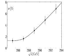
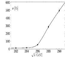
Figure 1: Cross sections at threshold for the reactions $e^{+}_{L}e^{-}_{R}\to{\tilde{e}}^{+}_{R}{\tilde{e}}^{-}_{R}$ (left) and $e^{-}_{R}e^{-}_{R}\to{\tilde{e}}^{+}_{R}{\tilde{e}}^{-}_{R}$ (right) in the SPS#1a scenario, including background [20]. Error bars correspond to a luminosity of $10~{}\mathrm{fb}^{-1}$ (left) and $1~{}\mathrm{fb}^{-1}$ (right) per point.

Slepton masses can be measured in threshold scans or in continuum. At threshold: $\tilde{\mu}^{+}_{L}\tilde{\mu}^{-}_{L}\,,\,\tilde{\mu}^{+}_{R}\tilde{\mu}^{-}_{R}\,,{\tilde{e}}_{L}^{+}{\tilde{e}}_{L}^{-}$ and ${\tilde{e}}_{R}^{+}{\tilde{e}}_{R}^{-}$ pairs are excited in a P-wave characterized by a slow rise of the cross section $\sigma\sim\beta^{3}$ with slepton velocity $\beta$. On the other hand, in $e_{L}^{+}e_{L}^{-}\,/\,e_{R}^{+}e_{R}^{-}\to{\tilde{e}}_{R}^{+}{\tilde{e}}_{L}^{-}\,/\,{\tilde{e}}_{L}^{+}{\tilde{e}}_{R}^{-}$ and $e_{L}^{-}e_{L}^{-}\,/\,e_{R}^{-}e_{R}^{-}\to{\tilde{e}}_{L}^{-}{\tilde{e}}_{L}^{-}\,/\,{\tilde{e}}_{R}^{-}{\tilde{e}}_{R}^{-}$ sleptons are excited in the S-wave giving steep rise of the cross sections $\sigma\sim\beta$. Therefore the shape of the cross section near threshold is sensitive to the masses and quantum numbers.

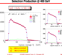
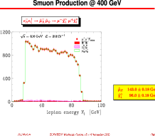
Figure 2: Lepton energy spectra in the processes $e^{-}_{R}e^{+}_{L}\to{\tilde{e}}^{-}_{R}\,{\tilde{e}}^{+}_{R}\to e^{-}\tilde{\chi}^{0}_{1}e^{+}\tilde{\chi}^{0}_{1}$ (left) and $e^{-}_{R}e^{+}_{L}\to{\tilde{\mu}}^{-}_{R}{\tilde{\mu}}^{+}_{R}\to\mu^{-}\tilde{\chi}^{0}_{1}\,\mu^{+}\tilde{\chi}^{0}_{1}\to\mu^{-}\tilde{\chi}^{0}_{1}\mu^{+}\tilde{\chi}^{0}_{1}$ (right) at $\sqrt{s}=400~{}\mathrm{GeV},{\cal L}=200~{}\mathrm{fb}^{-1}$; scenario SPS#1a [23].

The expected experimental precision requires higher order corrections, and finite sfermion width effects to be included. Examples of simulations for the SPS#1a point are shown in fig. 1. Using polarized $e^{+}e^{-}$ beams and ${\cal L}=50~{}\mathrm{fb}^{-1}$ a (highly correlated) 2-parameter fit gives $\delta m_{{\tilde{e}}_{R}}=0.20~{}\mathrm{GeV}$ and $\delta\Gamma_{{\tilde{e}}_{R}}=0.25~{}\mathrm{GeV}$; the resolution deteriorates by a factor of $\sim 2$ for ${\tilde{\mu}}_{R}{\tilde{\mu}}_{R}$ production. For $e^{-}_{R}e^{-}_{R}\to{\tilde{e}}_{R}{\tilde{e}}_{R}$ the gain in resolution is a factor $\sim 4$ with only a tenth of the luminosity, compared to $e^{+}e^{-}$ beams.

Above the threshold, slepton masses can be obtained from the endpoint energies of leptons coming from slepton decays. In the case of two-body decays, ${\tilde{\ell}}^{-}\to\ell^{-}\tilde{\chi}^{0}_{i}\$ and ${\tilde{\nu}}_{\ell}\to\ell^{-}\tilde{\chi}^{+}_{i}$ the lepton energy spectrum is flat with endpoints (the minimum $E_{-}$ and maximum $E_{+}$ energies)

$$E_{\pm} = {\textstyle\frac{1}{4}}\sqrt{s}\,(1\pm\beta)(1-{m_{\tilde{\chi}}^{2}}/{m_{{\tilde{\ell}}}^{2}})$$ (6)

providing an accurate determination of the masses of the primary slepton and the secondary neutralino/chargino.

Simulations of the $e$ and $\mu$ energy spectra of ${\tilde{e}}_{R}{\tilde{e}}_{R}$ and ${\tilde{\mu}}_{R}{\tilde{\mu}}_{R}$ (respectively) production, including beamstrahlung, QED radiation, selection criteria and detector resolutions, are shown in fig. 2 assuming mSUGRA scenario SPS#1a [23]. With a moderate luminosity of ${\cal L}=200~{}\mathrm{fb}^{-1}$ at $\sqrt{s}=400$ GeV one finds $m_{{\tilde{e}}_{R}}=143\pm 0.10$ GeV, $m_{{\tilde{\mu}}_{R}}=143\pm 0.10$ GeV and $m_{\tilde{\chi}^{0}_{1}}=96\pm 0.10$ GeV from selectron, or $m_{\tilde{\chi}^{0}_{1}}=96\pm 0.18$ GeV from smuon production processes. Assuming the neutralino mass is known, one can improve slepton mass determination by a factor 2 from reconstructed kinematically allowed minimum $m_{min}({\tilde{\ell}})$. A slightly better experimental error for the neutralino mass $\delta m_{\tilde{\chi}^{0}_{1}}=0.08$ GeV from the smuon production has recently been reported in [24]. The partner ${\tilde{\mu}}_{L}$ is more difficult to detect because of large background from $WW$ pairs and SUSY cascades. However, with the high luminosity of TESLA one may select the rare decay modes ${\tilde{\mu}}_{L}\to\mu\tilde{\chi}^{0}_{2}$ and $\tilde{\chi}^{0}_{2}\to\ell^{+}\ell^{-}\,\tilde{\chi}^{0}_{1}$, leading to a unique, background free signature $\mu^{+}\mu^{-}\,4\ell^{\pm}E\kern-6.00006pt/$. The achievable mass resolutions for $m_{{\tilde{\mu}}_{L}}$ and $m_{\tilde{\chi}^{0}_{2}}$ is of the order of 0.4 GeV [25].

One should keep in mind that the measurement of selectron masses is subject to two experimental difficulties: an overlap of flat energy distributions of leptons from ${\tilde{e}}_{R}^{-}{\tilde{e}}_{L}^{+},{\tilde{e}}_{R}^{-}{\tilde{e}}_{R}^{+},{\tilde{e}}_{L}^{-}{\tilde{e}}_{L}^{+},{\tilde{e}}_{L}^{-}{\tilde{e}}_{L}^{+}$, and large SM background. Nevertheless, it has been demonstrated [26] that thanks to larger cross sections, both problems can be solved by a double subtraction of $e^{-}$ and $e^{+}$ energy spectra and opposite electron beam polarizations ${\cal P}_{e^{-}}=+0.8$ and ${\cal P}_{e^{-}}=-0.8$, symbolically $(E_{e^{-}}-E_{e^{+}})_{e^{-}_{R}}-(E_{e^{-}}-E_{e^{+}})_{e^{-}_{L}}$. Such a procedure eliminates all charge symmetric background and clearly exhibits endpoints from the ${\tilde{e}}_{R}$ and ${\tilde{e}}_{L}$ decays, as seen in fig. 3. Simulations at $\sqrt{s}=500~{}\mathrm{GeV}$ in the SPS#1a scenario [26] show that both selectron masses can be determined to an accuracy of $\delta m_{{\tilde{e}}_{R},\,{\tilde{e}}_{L}}\sim 0.8~{}\mathrm{GeV}$.

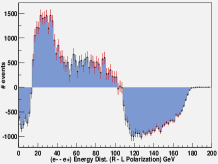
Figure 3: Energy spectrum $(E_{e^{-}}-E_{e^{+}})_{e^{-}_{R}}-(E_{e^{-}}-E_{e^{+}})_{e^{-}_{L}}$ for $e^{-}_{R,\,L}e^{+}\to{\tilde{e}}_{R}{\tilde{e}}_{L}$ in the model SPS#1a at $\sqrt{s}$=500 GeV, ${{\cal L}}$=2$\cdot$500 $\mathrm{fb}^{-1}$ [26].

2.2 Sneutrino production

At $e^{+}e^{-}$ collisions sneutrinos are produced in pairs via the s-channel $Z$ exchange; for the ${\tilde{\nu}}_{e}$ production there is additional t-channel chargino exchange. Their decay into the corresponding charged lepton and chargino, and the subsequent chargino decay, make the final topology, e.g. ${\tilde{\nu}}_{e}{\tilde{\nu}}_{e}\to e^{+}e^{-}\ell^{\pm}2j\,E\kern-6.00006pt/$, very clean. The primary charged lepton energy, and di-jet energy and mass spectra, see fig. 4, can be used to determine $m_{\tilde{\nu}}$ and $m_{\tilde{\chi}_{1}^{\pm}}$ to 2 per mil (or better), and to measure the chargino couplings and the $\tilde{\chi}^{\pm}_{1}-\tilde{\chi}^{0}_{1}$ mass difference; a resolution below 50 MeV, given essentially by detector systematics, appears feasible [25]. The detection and measurement of tau-sneutrinos ${\tilde{\nu}}_{\tau}$ is more problematic, due to neutrino losses in decay modes and decay energy spectra.

Figure 4: Lepton energy and di-jet mass spectra of $e^{-}_{L}e^{+}_{R}\to{\tilde{\nu}}_{e}{\tilde{\nu}}_{e}\to e^{-}\tilde{\chi}^{+}_{1}\,e^{+}\tilde{\chi}^{-}_{1}$ (left) with subsequent decay $\tilde{\chi}^{\pm}_{1}\to q\bar{q}^{\prime}\,\tilde{\chi}^{0}_{1}$ (right) [25]

2.3 Study of staus

In contrast to the first two generations, the $L-R$ mixing for the third generation sleptons can be non-negligible due to the large $\tau$ Yukawa coupling. Therefore the $\tilde{\tau}$’s are very interesting to study since their production and decay is different from $\tilde{e}$ and $\tilde{\mu}$.

The ${\tilde{\tau}}$ masses can be determined with the usual techniques of decay spectra or threshold scans at the per cent level, while the mixing angle $|\cos\theta_{\tilde{\tau}}|$ can be extracted with high accuracy from cross section measurements with different beam polarisations. In a case study [27] for $m_{\tilde{\tau}_{1}}=155$ GeV, $m_{\tilde{\tau}_{2}}=305$ GeV, $\mu=140$ GeV, $\tan\beta=20$, $A_{\tau}=-254$ GeV it has been found that at $\sqrt{s}=500$ GeV,  ${\cal L}=250$ fb^-1,  ${\cal P}_{e^{-}}=+0.8$,  ${\cal P}_{e^{+}}=-0.6$, the expected precision is as follows: $m_{\tilde{\tau}_{1}}=155\pm 0.8$ GeV,   $\cos 2\theta_{\tau}=-0.987\pm 0.08$, left panel of fig. 5.

The dominant decay mode $\tilde{\tau}_{1}\to\tilde{\chi}^{0}_{1}\tau$ can be exploited to determine $\tan\beta$ if $\tan\beta$ turns to be large [28]. In this case the non-negligible $\tau$ Yukawa coupling makes $\tilde{\tau}$ couplings sensitive to the neutralino composition in the decay process. Most importantly, if the higgsino component of the neutralino is sufficiently large, the polarization of $\tau$’s from the $\tilde{\tau}$ decay turns out to be a sensitive function of $\tilde{\tau}$ mixing, neutralino mixing and $\tan\beta$ [27]. This is crucial since for large $\tan\beta$ other SUSY sectors are not very sensitive to $\tan\beta$ and therefore cannot provide a precise determination of this parameter.

The $\tau$ polarization can be measured using the energy distributions of the decay hadrons, e.g. $\tau\to\pi\nu$ and $\tau\to\rho\nu\to\pi^{\pm}\pi^{0}\nu$. Simulations show that the $\tau$ polarization can be measured very accurately, $\delta{\cal P}_{\tau}=0.82\pm 0.03$, which in turn allows to determine $\tan\beta=20\pm 2$, as shown in the right panel of fig. 5.

$\cos 2\theta_{\tilde{\tau}}$                                  $\tan\beta$          

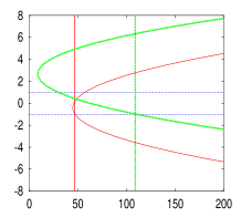
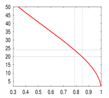
       $\sigma(e^{+}e^{-}\to{\tilde{\tau}}_{1}{\tilde{\tau}}_{1})$ [fb]                                     $P_{\tilde{\tau}_{1}\to\tau\tilde{\chi}^{0}_{1}}$

Figure 5: Left: $\cos 2\theta_{\tilde{\tau}}$ versus $\sigma(e^{+}e^{-}\to{\tilde{\tau}}_{1}{\tilde{\tau}}_{1})$ at $\sqrt{s}=500~{}\mathrm{GeV}$ for polarized (green, upper curve) and unpolarized (red, lower curve) beams; the expected cross sections shown by vertical lines. Unpolarised beams give a two-fold ambiguity in $\cos 2\theta_{\tilde{\tau}}$, while polarized beams give a unique physical solution. Right: $\tan{\beta}$ as a function of $\tau$ polarization. From simulations $P_{\tau}=0.82\pm 0.03$ leading to $\tan\beta=22\pm 2$ [27].

2.4 Squarks

For the third generation squarks, $\tilde{t}$ and $\tilde{b}$,   the $L-R$ mixing is also expected to be important. As a result of the large top quark Yukawa coupling, it is possible that the lightest superpartner of the quarks is the stop ${\tilde{t}}_{1}={\tilde{t}}_{L}\cos\theta_{\tilde{t}}+{\tilde{t}}_{R}\sin\theta_{\tilde{t}}$. If the mass $m_{{\tilde{t}}_{1}}$ is below 250 GeV, it may escape detection at the LHC, while it can easily be discovered at the Linear Collider.

$\cos\theta_{\tilde{t}}$                                          $\tan\beta$
          
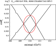
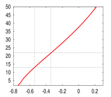
         $m_{\tilde{t}}$ [GeV]                                            $P_{{\tilde{b}}_{1}\to t\tilde{\chi}_{1}^{\pm}}$

Figure 6: Left: Contours of $\sigma_{R}({\tilde{t}}_{1}{\tilde{t}}_{1})$ and $\sigma_{L}({\tilde{t}}_{1}{\tilde{t}}_{1})$ as a function of $m_{{\tilde{t}}_{1}}$ and $\cos\theta_{\tilde{t}}$ for $\sqrt{s}=500~{}\mathrm{GeV}$, ${\cal L}=2\cdot 500~{}\mathrm{fb}^{-1}$ [29]. Right: $\tan\beta$ as a function of top polarization. From simulations $P_{t}=-0.44\pm 0.10$ leading to $\tan\beta=17.5\pm 4.5$ [27].

The ${\tilde{t}}$ and ${\tilde{b}}$ phenomenology is analogous to that of the ${\tilde{\tau}}$ system. The masses and mixing angles can be extracted from production cross sections measured with polarized beams. The production cross sections for $e^{+}e^{-}\to{\tilde{t}}_{1}\bar{\tilde{t}}_{1}$ with different beam polarizations, $\sigma_{R}=\sigma_{e^{-}_{R}e^{+}_{L}}$ and $\sigma_{L}=\sigma_{e^{-}_{L}e^{+}_{R}}$, have been studied for ${\tilde{t}}_{1}\to b\,\tilde{\chi}^{\pm}_{1}$ and ${\tilde{t}}_{1}\to c\,\tilde{\chi}^{0}_{1}$ decay modes including full-statistics SM background. New analyses have been performed for the SPS#5-type point: a dedicated “light-stop” scenario with $m_{{\tilde{t}}_{1}}=210$ GeV, $m_{\tilde{\chi}^{0}_{1}}=121.2$ GeV [29]. For this point the decay ${\tilde{t}}_{1}\to b\,\tilde{\chi}^{\pm}_{1}$ is not open, and the SUSY background is small. The charm tagging, based on a CCD detector, helps to enhance the signal from the decay process ${\tilde{t}}_{1}\to c\,\tilde{\chi}^{0}_{1}$. Generated events were passed through the SIMDET detector simulation. The results, shown in the left panel of fig. 6, provide high accuracies on the mass $\Delta m_{{\tilde{t}}_{1}}\sim 0.7$ GeV and mixing angle $\Delta\cos\theta_{\tilde{t}}\sim 0.01$.

If the heavier stop ${\tilde{t}}_{2}$ is too heavy to be produced at the LC, the precise measurement of the Higgs boson mass $m_{h}$ together with measurements from the LHC can be used to obtain indirect limits on $m_{{\tilde{t}}_{2}}$ [30]. Assuming $m_{{\tilde{t}}_{1}}=180\pm 1.25$ GeV, $\cos\theta_{\tilde{t}}=0.57\pm 0.01$, $M_{A}=257\pm 10$ GeV, $\mu=263\pm 1$ GeV, $m_{\tilde{g}}=496\pm 10$ GeV, $A_{\tilde{b}}=A_{\tilde{t}}\pm 30\%$ and $m_{{\tilde{b}}_{1}}>200$ GeV, fig. 7 shows the allowed region in the $m_{{\tilde{t}}_{2}}$–$m_{h}$ plane. Only a lower bound $\tan\beta>10$ has been assumed, which could for instance be inferred from the gaugino/higgsino sector.

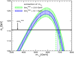
Figure 7: Indirect determination of $m_{{\tilde{t}}_{2}}$ from the $m_{h}$ measurement for $\delta m_{t}$=2 GeV (LHC) and 0.1 GeV (LC) [30].                                                

Intersection of the assumed measured value $m_{h}=115.5\pm 0.05$ GeV with the allowed $m_{{\tilde{t}}_{2}}$–$m_{h}$ region gives an indirect determination of $m_{{\tilde{t}}_{2}}$, yielding 670 GeV $\;\raisebox{-3.87495pt}{$\textstyle\stackrel{{\scriptstyle\textstyle<}}{{\sim}}$}\;m_{{\tilde{t}}_{2}}\;\raisebox{-3.87495pt}{$\textstyle\stackrel{{\scriptstyle\textstyle<}}{{\sim}}$}\;$ 705 GeV for the LHC precision $\delta m_{t}=2$ GeV (${{\tilde{t}}_{2}}$ must be above the LC reach). The LC precision of $\delta m_{t}=0.1$ GeV reduces the range to 680 GeV $\;\raisebox{-3.87495pt}{$\textstyle\stackrel{{\scriptstyle\textstyle<}}{{\sim}}$}\;m_{{\tilde{t}}_{2}}\;\raisebox{-3.87495pt}{$\textstyle\stackrel{{\scriptstyle\textstyle<}}{{\sim}}$}\;$ 695 GeV, i.e. by a factor of more than 2.

Similarly to the ${\tilde{\tau}}$, the measurement of top quark polarization in the squark decay can provide information on $\tan\beta$. For this purpose the decay $\tilde{b}_{1}\to t\tilde{\chi}^{\pm}_{1}$ is far more useful than $\tilde{t}_{1}\to t\tilde{\chi}^{0}_{k}$ since in the latter the $t$ polarization depends on $1/\sin\beta$ and therefore is only weakly sensitive to large $\tan\beta$.

A feasibility study of the reaction

$$e^{+}_{L}e^{-}_{R} \to {\tilde{b}}_{1}\bar{\tilde{b}}_{1}\ \to\ t\tilde{\chi}_{1}^{-}+\bar{t}\tilde{\chi}_{1}^{+}\quad\$$ (7)

has been performed in [27]. A fit to the angular distribution $\cos\theta^{*}_{s}$, where $\theta^{*}_{s}$ is the angle between the $\bar{s}$ quark and the primary ${\tilde{b}}_{1}$ in the top rest frame in the decay chain $e^{+}e^{-}\to\bar{\tilde{b}}_{1}+t\,\tilde{\chi}_{1}^{-}\to\bar{\tilde{b}}_{1}+bc\bar{s}\,\tilde{\chi}_{1}^{-}$, yields $P_{t}=-0.44\pm 0.10$, consistent with the input value of $P_{t}^{th}=-0.38$. From such a measurement one can derive $\tan\beta=17.5\pm 4.5$, as illustrated in the right panel of fig. 6. After $\tan\beta$ is fixed, measurements of stop masses and mixing allow us to determine the trilinear coupling $A_{\tilde{t}}$ at the ten-percent level [27].

2.5 Quantum numbers

An important quantity is the spin of the sfermion which can directly be determined from the angular distribution of sfermion pair production in $e^{+}e^{-}$ collisions [1, 25].

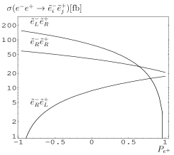
Figure 8: Production cross sections as a function of $P_{e^{+}}$ for $\sqrt{s}$ =350 GeV, $P_{e^{-}}$=-0.8. ISR and beamstrahlung are included [31].                                                             

Due to small $L-R$ mixing of the first two generation sfermions, the mass eigenstates are chiral. As a result, of particular interest is the associated production of

$$e^{-}_{R}e^{+}_{R}\to{\tilde{e}}_{R}^{-}{\tilde{e}}_{L}^{+} {\rm and} e^{-}_{L}e^{+}_{L}\to{\tilde{e}}_{L}^{-}{\tilde{e}}_{R}^{+}$$ (8)

via $t$-channel $\tilde{\chi}^{0}$ exchange for the sfermion quantum number determination. For polarized beams the charge of the observed lepton is directly associated to the $L,\,R$ quantum numbers of the selectrons and the energy spectrum uniquely determines whether it comes from the ${\tilde{e}}_{R}$ or the ${\tilde{e}}_{L}$ decay. However, in order to separate the t-channel neutralino exchange from the s-channel photon and Z-boson exchange, both the electron and positron beams must be polarized. By comparing the selectron cross-section for different beam polarizations the chiral quantum numbers of the selectrons can be disentangled, as can be seen in fig. 8, where other parameters are $m_{\tilde{e}_{R}}=137.7$ GeV, $m_{\tilde{e}_{L}}=179.3$ GeV, $M_{2}=156$ GeV, $\mu=316$ GeV and $\tan\beta=3$ [31].

2.6 Sfermion Yukawa couplings

Supersymmetry enforces gauge couplings and their supersymmetric Yukawa counterparts to be exactly equal at tree level. For example, the Yukawa coupling $\hat{g}_{\tilde{V}f\tilde{f}}$ between the gaugino partner $\tilde{V}$ of the vector boson $V$, the fermion $f$ and the sfermion $\tilde{f}$ must be equal to the corresponding gauge coupling $g_{Vff}$.

The Yukawa couplings of selectrons can best be probed in the production of selectrons via the t-channel neutralino exchange contributions. For this purpose one can exploit the $e^{-}e^{-}$ collider mode due to reduced background, larger production cross-sections, higher beam polarizability and no interfering s-channel contributions. Simulations have shown that these couplings can be determined with high accuracy [20, 32]. For example, errors for the extraction of the supersymmetric Yukawa couplings $\hat{g}_{1}$ and $\hat{g}_{2}$ (corresponding to the U(1) and SU(2) gauge couplings $g_{1}$ and $g_{2}$) are expected in the range $\delta\hat{g}_{1}/\hat{g}_{1}\approx 0.2\%$ and $\delta\hat{g}_{2}/\hat{g}_{2}\approx 0.8\%$. The values are for the SPS#1a scenario and integrated luminosity of 50 fb^-1 of the $e^{-}e^{-}$ collider running at $\sqrt{s}=500\mathrm{GeV}$, with no detector simulation included. Similar precision in the $e^{+}e^{-}$ mode requires integrated luminosity of 500 fb^-1, see fig. 9.

Figure 9: The 1$\sigma$ bounds on the supersymmetric Yukawa couplings $\hat{g}_{1}$ and $\hat{g}_{2}$ in the SPS#1a scenario from $e^{-}e^{-}$ with ${\cal L}=50$ fb^-1 (left) and $e^{+}e^{-}$ with ${\cal L}=500$ fb^-1 (right), both running at $\sqrt{s}=500$ GeV [32].

Such a high experimental precision requires radiative corrections to be included in the theoretical predictions for the slepton cross-sections. Far above threshold the effects of the non-zero slepton width are small, of the order $\Gamma_{\tilde{f}}/m_{\tilde{f}}$, and the production and decay of the sleptons can be treated separately. As mentioned, for both sub-processes the complete electroweak one-loop corrections in the MSSM have been computed [20, 21]. The electroweak corrections were found to be sizable, of the order of 5–10%. They include important effects from supersymmetric particles in the virtual corrections, in particular non-decoupling logarithmic contributions, e.g. terms $\propto\log m_{\tilde{f}}/m_{\rm weak}$ from fermion-sfermion-loops.

The equality of gauge and Yukawa couplings in the SU(3)_C gauge sector can be tested at a linear collider by investigating the associated production of quarks $q$ and squarks $\tilde{q}$ with a gluon $g$ or gluino $\tilde{g}$. While the processes $e^{+}e^{-}\to q\bar{q}g$ and $e^{+}e^{-}\to\tilde{q}\bar{\tilde{q}}g$ are sensitive to the strong gauge coupling of quarks and squarks, respectively, the corresponding Yukawa coupling can be probed in $e^{+}e^{-}\to q\bar{\tilde{q}}\tilde{g}$. In order to obtain reliable theoretical predictions for these cross-sections it is necessary to include next-to-leading order (NLO) supersymmetric QCD corrections. These corrections are generally expected to be rather large and they are necessary to reduce the large scale dependence of the leading-order result. The NLO QCD corrections to the process $e^{+}e^{-}\to q\bar{q}g$ within the Standard Model have been known for a long time. Recently, the complete ${\cal O}(\alpha_{\rm s})$ corrections to all three processes in the MSSM have been calculated [33]. The NLO contributions enhance the cross-section in the peak region by roughly 20% with respect to the LO result. Furthermore, the scale dependence is reduced by a factor of about six when the NLO corrections are included.

2.7 Mass universality

Most analyses are performed with a simplifying assumption of universal mass parameters at some high energy scale $G$: $\delta m^{2}(G)=m^{2}_{\tilde{l}_{R}}(G)-m^{2}_{\tilde{l}_{L}}(G)$=0. This assumption can be tested at the LC. For example, in [34] a quantity

$$\Delta^{2}= m^{2}_{\tilde{e}_{R}}-m^{2}_{\tilde{e}_{L}}+\frac{m^{2}_{\tilde{\chi}^{\pm}_{1}}}{2\alpha^{2}_{2}}[\frac{3}{11}(\alpha^{2}_{1}-\alpha^{2}_{1}(G))$$ (9)

$$-3(\alpha_{2}^{2}-\alpha^{2}_{2}(G))],$$

defined at the electroweak scale, is proposed as a probe of non-universality of slepton masses if only both selectrons and the light chargino are accessible at a linear collider ($\alpha_{1}$ and $\alpha_{2}$ are the U(1) and SU(2) couplings). It turns out that $\Delta^{2}$ is strongly correlated with the slepton mass splitting, $\Delta^{2}\sim 0.76\;\delta m^{2}(G)$. Assuming SUSY masses in the 150 GeV range to be measured with an experimental error of 1%, it has been found [34] that the non-universality can be detected for $|\delta m^{2}(G)|\geq 2500$ GeV²; knowing the gaugino mass $M_{2}$ to 1% increases the sensitivity down to $\delta m^{2}(G)=1400$ GeV².

2.8 Sfermions with complex CP phases

The soft SUSY breaking parameters: the gaugino masses and trilinear scalar couplings, and the Higgsino mass parameter $\mu$, can in general be complex and the presence of non-trivial phases violates CP. This generalization is quite natural and is motivated by the analogy between fermions and sfermions: in the SM the CKM phase is quite large and the smallness of CP-violating observables results from the structure of the theory. Furthermore, large leptonic CP-violating phases together with leptogenesis may explain the baryonic asymmetry of the Universe.

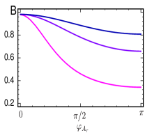
Figure 10: Branching ratios of ${\tilde{\tau}}_{1}\to\tilde{\chi}^{0}_{1}\tau$ for $m_{{\tilde{\nu}}}=233$, $238$, $243$ GeV (from bottom to top) [37].                                                        

In mSUGRA-type models the phase $\varphi_{\mu}$ of $\mu$ is restricted by the experimental data on electron, neutron and mercury electric dipole moments (EDMs) to a range $|\varphi_{\mu}|\;\raisebox{-3.87495pt}{$\textstyle\stackrel{{\scriptstyle\textstyle<}}{{\sim}}$}\;0.1$ – 0.2 if a universal scalar mass parameter $M_{0}\;\raisebox{-3.87495pt}{$\textstyle\stackrel{{\scriptstyle\textstyle<}}{{\sim}}$}\;400$ GeV is assumed. However, the restriction due to the electron EDM can be circumvented if complex lepton flavour violating terms are present in the slepton sector [35]. The phases of the parameters $A_{{\tilde{t}},{\tilde{b}}}$ enter the EDM calculations only at two-loop level, resulting in much weaker constraints [36].

Figure 11: Left: Branching ratios of ${\tilde{t}}_{1}\to\tilde{\chi}^{+}_{1}b$ (solid), $\tilde{t}_{1}\to\tilde{\chi}^{0}_{1}t$ (dashed), $\tilde{t}_{1}\to\tilde{\chi}^{+}_{2}b$ (dashdotted). Right: Contours of $B(\tilde{t}_{1}\to\tilde{\chi}^{0}_{1}t)$ in the SPS#1a inspired scenario. The dashed lines denote the contours of $\cos\theta_{\tilde{t}}$ [38].

In the pure sfermionic sector the phases of $A_{\tilde{f}}$ and $\mu$, eq. (5), enter the masses $m_{{\tilde{f}}_{1,2}}^{2}$ and mixing angle $\theta_{\tilde{f}}$ only through a term $m_{f}^{2}|A_{\tilde{f}}\mu|(\tan\beta)^{-2I^{3}_{f}}\cos(\varphi_{A_{\tilde{f}}}+\varphi_{\mu})$. Therefore the ${\tilde{t}}_{1,2}$ masses are more sensitive to phases than masses of ${{\tilde{\tau}}_{1,2}}$ and ${\tilde{b}}_{1,2}$ because of the mass hierarchy of the corresponding fermions. The phase dependence of $\theta_{\tilde{f}}$ is strongest if $|A_{\tilde{f}}|\simeq|\mu|(\tan\beta)^{-2I^{3}_{f}}$ and $|m_{{\tilde{f}}_{L}}^{2}-m_{{\tilde{f}}_{R}}^{2}|\;\raisebox{-3.87495pt}{$\textstyle\stackrel{{\scriptstyle\textstyle<}}{{\sim}}$}\;|a_{\tilde{f}}m_{f}|$ [37]. Since the $Z{\tilde{f}}_{i}{\tilde{f}}_{i}$ couplings are real, and for${\tilde{f}}_{1}\bar{{\tilde{f}}}_{2}$ production only $Z$ exchange contributes, the ${\tilde{f}}_{i}\bar{{\tilde{f}}}_{j}$ production cross sections do not explicitly depend on the phases – dependence enters only through the shift of sfermion masses and mixing angle. However, the various $\tilde{f}$ decay branching ratios depend in a characteristic way on the complex phases. This is illustrated in fig. 10, where branching ratios for ${\tilde{\tau}}_{1}$ are shown for $m_{{\tilde{\tau}}_{1}}=240$ GeV, $\mu=300$ GeV, $|A_{\tilde{\tau}}|=1000$ GeV, $\tan\beta=3$, and $M_{2}=200$ GeV [37]. The branching ratios for the light ${\tilde{t}}_{1}$ in the SPS#1a inspired scenario are shown in fig. 11, including the contour plot for the mixing angle $\cos\theta_{\tilde{t}}$ [38]. A simultaneous measurement of $B(\tilde{t}_{1}\to\tilde{\chi}^{0}_{1}t)$ and $\cos\theta_{\tilde{t}}$ might be helpful to disentangle the phase of $A_{\tilde{t}}$ from its absolute value. As an example a measurement of $B(\tilde{t}_{1}\to\tilde{\chi}^{0}_{1}t)=0.6\pm 0.1$ and $|\cos\theta_{\tilde{t}}|=0.3\pm 0.02$ would allow to determine $|A_{\tilde{t}}|\approx 320$ GeV with an error $\Delta(|A_{\tilde{t}}|)\approx 20$ GeV and $\varphi_{A_{\tilde{t}}}$ with a twofold ambiguity $\varphi_{A_{\tilde{t}}}\approx 0.35\pi$ or $\varphi_{A_{\tilde{t}}}\approx 1.65\pi$ with an error $\Delta(\varphi_{A_{\tilde{t}}})\approx 0.1\pi$, see fig. 11 (right).

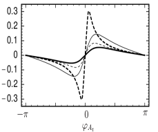
Figure 12: The $CP$ sensitive asymmetry as a function of $\varphi_{A_{\tilde{t}}}$; $\tan\beta$=3 (thick), $\tan\beta$=10 (thin), $\mu$=400 GeV (solid), $\mu$=700 GeV (dashed) [39].

In principle, the imaginary parts of the complex parameters involved could most directly and unambiguously be determined by measuring suitable $CP$ violating observables. For example, the polarization of the $\tau^{+}$ normal to the $\tilde{t}_{1}$ decay plane in the decay $\tilde{t}_{1}\to b{\tilde{\nu}}\tau^{+}$ is sensitive to $CP$ violation. The asymmetry of the $\tau$ polarization perpendicular to the decay plane can go up to $30\%$ for some SUSY parameter points where the decay $\tilde{t}_{1}\to b{\tilde{\nu}}\tau^{+}$ has a sufficient branching ratio allowing for the measurement of this asymmetry, see fig. 12 where other parameters are taken as $m_{{\tilde{t}}_{1}}=240$ GeV, $m_{{\tilde{t}}_{2}}=800$ GeV, $m_{{\tilde{\nu}}}=200$ GeV, $M_{2}=350$ GeV, $|A_{\tilde{t}}|=1000$ GeV [39].

CP violation in the stau sector can generate electric and weak dipole moments of the taus. The CP-violating tau dipole form factors can be detected up to the level of $(3-5)\cdot 10^{-19}e{\rm cm}$ [40] at a linear collider with high luminosity and polarization of both $e^{+}$ and $e^{-}$ beams. Although such a precision would improve the current experimental bounds by three orders of magnitude, it still remains by an order of magnitude above the expectations from supersymmetric models with CP-violation.

2.9 Lepton flavour violation

There are stringent constraints on lepton flavour violation (LFV) in the charged lepton sector, the strongest being $BR(\mu^{-}\to e^{-}\gamma)<1.2\times 10^{-11}$ [41]. However, neutrino oscillation experiments have established the existence of LFV in the neutrino sector with $\tan^{2}\theta_{Atm}\simeq 1$, $\tan^{2}\theta_{\odot}=0.24-0.89$ and $\sin^{2}(2\theta_{13})\;\raisebox{-3.87495pt}{$\textstyle\stackrel{{\scriptstyle\textstyle<}}{{\sim}}$}\;0.1$ [42].

$\sigma(e^{\pm}\tau^{\mp}E\kern-5.40005pt/)$ [fb]                       $\Delta m_{23}$ [GeV]

BR$(\tau\to e\gamma)$                                          $\sin 2\theta_{23}$

Figure 13: Left: Cross section for the signal $e^{\pm}\tau^{\mp}E\kern-6.00006pt/$ as a function of BR$(\tau\to e\gamma)$ for $\sqrt{s}=500$ GeV [45]. Right: 3$\sigma$ significance contours for $\sqrt{s}=$500 GeV and $\int{\cal L}$= 500 fb^-1 (A), =1000 fb^-1 (B). Line C: $\tilde{\nu}\tilde{\nu}^{*}$ contribution with luminosity 500 fb^-1. Dotted lines: BR($\tau\to\mu\gamma$)=10^-7, 10^-8, 10^-9 [46].

In the MSSM the R–parity symmetry forces total lepton number conservation but still allows the violation of individual lepton number, e.g. due to loop effects in $\mu^{-}\to e^{-}\gamma$ [43]. Moreover, a large $\nu_{\mu}$-$\nu_{\tau}$ mixing can lead to a large $\tilde{\nu}_{\mu}$-$\tilde{\nu}_{\tau}$ mixing via renormalization group equations. Therefore one can expect clear LFV signals in slepton and sneutrino production and in the decays of neutralinos and charginos into sleptons and sneutrinos at future colliders [44].

For the reference point SPS#1a a scan over the flavour non-diagonal ($i\neq j$) entries of slepton mass matrix eq. (2) shows [45] that values for $|M^{2}_{R,ij}|$ up to $8\cdot 10^{3}$ GeV², $|M^{2}_{L,ij}|$ up to $6\cdot 10^{3}$ GeV² and $|A_{ij}v_{d}|$ up to 650 GeV² are compatible with the current experimental constraints. In most cases, one of the mass squared parameters is at least an order of magnitude larger than the others. However, there is a sizable part in parameter space where at least two of the off-diagonal entries have the same order of magnitude.

Possible LFV signals at an $e^{+}e^{-}$ collider include $e\mu\,E\kern-6.00006pt/$, $e\tau\,E\kern-6.00006pt/$, $\mu\tau\,E\kern-6.00006pt/$ in the final state plus a possibility of additional jets. In fig. 13 the cross section of $e^{+}e^{-}\to e^{\pm}\tau^{\mp}E\kern-6.00006pt/$ at $\sqrt{s}=500$ GeV versus BR($\tau\to e\gamma$) is shown for points consistent with the experimental LFV data which are randomly generated in the range $10^{-8}\leq|A_{ij}|\leq 50$ GeV, $10^{-8}\leq M^{2}_{ij}\leq 10^{4}$ GeV². The accumulation of points along a band is due to a large $\tilde{e}_{R}$-$\tilde{\tau}_{R}$ mixing which is less constrained by $\tau^{-}\to e^{-}\gamma$ than the corresponding left-left or left-right mixing.

Note that the collider LFV signals can be very competitive to those from rare charged lepton decay, like $\tau\to\mu\gamma$. This is illustrated in fig. 13, where for simplicity the LFV has been restricted to the 2-3 generation subspace of sneutrinos with the mixing angle $\theta_{23}$ and $\Delta m_{23}=|m_{{\tilde{\nu}}_{2}}-m_{{\tilde{\nu}}_{3}}|$ as free parameters. [46].

2.10 Sgoldstinos

In the GMSB SUSY, not only the mass splittings $\Delta m^{2}$, but also the supersymmetry-breaking scale $\sqrt{F}$ is close to the weak scale: $G_{F}^{-1/2}\sim\Delta m^{2}\;\raisebox{-3.87495pt}{$\textstyle\stackrel{{\scriptstyle\textstyle<}}{{\sim}}$}\;\sqrt{F}$. Then the gravitino $\tilde{G}$ becomes very light, with $m_{\tilde{G}}={F}/{\sqrt{3}M^{\prime}_{P}}={F}/{(10~{}{\rm TeV})^{2}}\times 0.03$ eV. The appropriate effective low-energy theory must then contain, besides the goldstino, also its supersymmetric partners, called sgoldstinos [47]. The spin-0 complex component of the chiral goldstino superfield has two degrees of freedom, giving rise to two sgoldstino states: a CP-even state $S$ and a CP-odd state $P$. In the simplest case it is assumed that there is no sgoldstino-Higgs mixing, and that squarks, sleptons, gluinos, charginos, neutralinos and Higgs bosons are sufficiently heavy not to play a rôle in sgoldstino production and decay. Thus the $S$ and $P$ are mass eigenstates and, being R–even, they can be produced singly together with the SM particles.

During the Workshop new results on massive sgoldstino production at $e^{+}e^{-}$ and $\gamma\gamma$ colliders have been presented [48]. The most interesting channels for the production of such scalars ($\phi$ will be used to indicate a generic state) are the process $e^{+}e^{-}\to\phi\gamma$, and the fusion $\gamma\gamma\to\phi$, followed by the $\phi$ decay to photons or gluons.

The $e^{+}e^{-}\to\phi\gamma\to gg\gamma$ process gives rise to events with one monochromatic photon and two jets. However, the brems- and beamstrahlung induces a photon energy smearing comparable to or larger than the experimental resolution. On the other hand, the signal can be searched for directly in the jet-jet invariant mass distribution. Results of the simulation are presented in fig. 14 where the exclusion region at the 95% CL is shown in the $m_{\phi}$–$\sqrt{F}$ plane for two parameter sets: 1) $M_{1}$ = 200 GeV, $M_{2}$ = 300 GeV, $M_{3}$ = 400 GeV, 2) $M_{1}=M_{2}=M_{3}$ = 350 GeV.

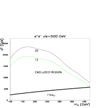
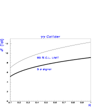
Figure 14: Left: Exclusion region at 95% CL at a 500 GeV $e^{+}e^{-}$ collider. Right: Exclusion region at 95% CL and 5$\sigma$ discovery at a $\gamma\gamma$ collider [48].

For the $\gamma\gamma$ collider, despite the smaller decay branching ratio, only the two-photon final state has been considered since it has a very little SM background. Taking as a reference point the value $(\sigma B)_{0}$ obtained for $M_{\gamma\gamma}=350$ GeV and a 10$\%$ branching ratio to two photons, the 95 % CL exclusion limit on and the $5~{}\sigma$ discovery line for $\sqrt{F}$ is shown in fig. 14 in terms of the ratio $R=\sigma\times BR(\phi\rightarrow\gamma\gamma)/(\sigma B)_{0}$. Thus the sensitivity at a photon collider obtained from the same electron-positron beam energy is expected to be much higher for $m_{\phi}\sim 300-400$ GeV.

3 GAUGINOS AND HIGGSINOS

Supersymmetric partners of electroweak gauge and Higgs bosons mix due to the gauge symmetry breaking. The mass-eigenstates (with positive mass eigenvalues) are charginos ($\tilde{\chi}^{\pm}_{i}$, $i$=1,2, mixtures of the wino and charged higgsino) and neutralinos ($\tilde{\chi}^{0}_{i}$, $i$=1,2,3,4, mixtures of $\tilde{B}$, $\tilde{W}^{3}$, $\tilde{H}_{1}^{0}$ and $\tilde{H}_{2}^{0}$). At tree level the chargino sector depends on $M_{2}$, $\mu$ and $\tan\beta$; the neutralino sector depends in addition on $M_{1}$. The gaugino and higgsino mass parameters can be complex; without loss of generality $M_{2}$ can be assumed real and positive, and the non-trivial CP-violating phases may be attributed to $\mu=|\mu|e^{i\varphi_{\mu}}$ and $M_{1}=|M_{1}|e^{i\varphi_{1}}$. The chargino mass matrix is diagonalized by two unitary matrices acting on left- and right-chiral weak eigenstates (parameterized by two mixing angles $\phi_{L,R}$ and three CP phases $\beta_{L,R}$ and $\gamma$) [49, 50]. The neutralino mass matrix is diagonalized by a 4$\times$4 unitary rotation $N$ parameterized in terms of 6 angles and 9 phases (three Majorana $\alpha_{i}$ and six Dirac $\beta_{ij}$ phases) [51, 52]

$$N={\rm diag}\{1,\,{\rm e}^{i\alpha_{1}},{\rm e}^{i\alpha_{2}},{\rm e}^{i\alpha_{3}}\}{\rm R}_{34}\,{\rm R}_{24}\,{\rm R}_{14}\,{\rm R}_{23}\,{\rm R}_{13}\,{\rm R}_{12}$$ (10)

where ${\rm R}_{jk}$ are rotations in the [$jk$] plane characterized by a mixing angle $\theta_{jk}$ and a (Dirac) phase $\beta_{jk}$.

Charginos and neutralinos are produced in pairs

$$e^{+}e^{-} \to \tilde{\chi}^{+}_{i}\tilde{\chi}^{-}_{j},\quad\tilde{\chi}^{0}_{i}\tilde{\chi}^{0}_{j}$$ (11)

via $s$-channel $\gamma/Z$ and $t$-channel ${\tilde{\nu}}_{e}$ exchange for $\tilde{\chi}^{\pm}$, and via $s$-channel $Z$ and $t$- and $u$-channel ${\tilde{e}}$ exchange for $\tilde{\chi}^{0}$ production. Beam polarizations are very important to study the $\tilde{\chi}$ properties and couplings. The polarized differential cross section for the $\tilde{\chi}_{i}\tilde{\chi}_{j}$ production can be written as [52]

$$\frac{{\rm d}\sigma^{\{ij\}}}{{\rm d}\cos\theta\,{\rm d}\phi}=\frac{\alpha^{2}\lambda^{1/2}}{16\,s}[(1-P_{l}\bar{P}_{l})\Sigma_{u}+(P_{l}-\bar{P}_{l})\Sigma_{l}$$

$$+P_{t}\bar{P}_{t}\cos(2\phi-\eta)\Sigma_{t}+P_{t}\bar{P}_{t}\sin(2\phi-\eta)\Sigma_{n}]\$$ (12)

where $\lambda=[1-(\mu_{i}+\mu_{j})^{2}][1-(\mu_{i}-\mu_{j})^{2}]$ is the two–body phase space function with $\mu_{i}=m_{\tilde{\chi}_{i}^{0}}/\sqrt{s}$, $P$=$(P_{t},0,P_{l})$ [$\bar{P}$=$(\bar{P}_{t}\cos\eta,\bar{P}_{t}\sin\eta,-\bar{P}_{l})$] is the electron [positron] polarization vector; the electron–momentum direction defines the $z$–axis and the electron transverse polarization–vector the $x$–axis. The coefficients $\Sigma_{u}$, $\Sigma_{l}$, $\Sigma_{t}$ and $\Sigma_{n}$ depend only on the polar angle $\theta$ and their explicit form is given in [50] for charginos, and in [52] for neutralinos. The $\Sigma_{n}$, present only for non-diagonal neutralino production, is particularly interesting because it is non-vanishing only in the CP-violating case.

Given the high experimental precision in mass and cross section measurements expected at the LC, the radiative corrections will have to be applied to the above expressions. Recently full one-loop corrections to chargino and neutralino sector have been calculated [21, 53, 54, 55]. The numerical analysis based on a complete one loop calculation has shown that the corrections to the chargino and neutralino masses can go up to 10% and the change in the gaugino and higgsino components can be in the range of 30%, and therefore will have to be taken into account.

3.1 Charginos

Experimentally the chargino masses can be measured very precisely at threshold since the production cross section for spin 1/2 Dirac fermions rises as $\beta$ leading to steep excitation curves. Results of a simulation for the reaction $e^{+}_{R}e^{-}_{L}\to\tilde{\chi}^{+}_{1}\tilde{\chi}^{-}_{1}\to\ell^{\pm}\nu_{\ell}\tilde{\chi}^{0}_{1}\,q\bar{q}^{\prime}\tilde{\chi}^{0}_{1}$, fig. 15, show that the mass resolution is excellent of ${\cal O}(50~{}\mathrm{MeV})$, degrading to the per mil level for the higher $\tilde{\chi}^{\pm}_{2}$ state. Above threshold, from the di-jet energy distribution one expects a mass resolution of $\delta m_{\tilde{\chi}_{1}^{\pm}}=0.2~{}\mathrm{GeV}$, while the di-jet mass distributions constrains the $\tilde{\chi}^{\pm}_{1}-\tilde{\chi}^{0}_{1}$ mass splitting within about $100~{}\mathrm{MeV}$.

Figure 15: Cross section for $e^{+}_{R}e^{-}_{L}\to\tilde{\chi}^{+}_{1}\tilde{\chi}^{-}_{1}\to\ell^{\pm}\nu_{\ell}\tilde{\chi}^{0}_{1}\,q\bar{q}^{\prime}\tilde{\chi}^{0}_{1}$ at threshold (in the RR 1 scenario [1, 25], errors for $10~{}\mathrm{fb}^{-1}$ per point).

Since the chargino production cross sections are simple binomials of $\cos 2\phi_{L,R}$, see fig. 16, the mixing angles can be determined in a model independent way using polarized electron beams [56].

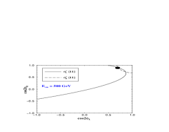
Figure 16: Contours of $\sigma(\tilde{\chi}^{+}_{1}\tilde{\chi}^{-}_{1})$ with polarized beams in the plane $[\cos 2\phi_{L},\cos 2\phi_{R}]$ [56].                                                       

Once masses and mixing angles are measured, the fundamental SUSY parameters of the chargino sector can be extracted to lowest order in analytic form [56, 57]

$$M_{2}=M_{W}[\Sigma-\Delta[\cos 2\phi_{R}+\cos 2\phi_{L}]]^{1/2}$$ (13)

$$\left|\mu\right|=M_{W}[\Sigma+\Delta[\cos 2\phi_{R}+\cos 2\phi_{L}]]^{1/2}$$ (14)

$$\cos\Phi_{\mu}=[\Delta^{2}-(M^{2}_{2}-\mu^{2})^{2}-4m^{2}_{W}(M^{2}_{2}+\mu^{2})\qquad{}$$

$$\qquad\qquad-4m^{4}_{W}\cos^{2}2\beta]/8m_{W}^{2}M_{2}|\mu|\sin 2\beta$$ (15)

$$\tan\beta=\left[\frac{1+\Delta(\cos 2\phi_{R}-\cos 2\phi_{L})}{1-\Delta(\cos 2\phi_{R}-\cos 2\phi_{L})}\right]^{1/2}$$ (16)

where $\Delta=(m^{2}_{\tilde{\chi}^{\pm}_{2}}-m^{2}_{\tilde{\chi}^{\pm}_{1}})/4M^{2}_{W}$ and $\Sigma=(m^{2}_{\tilde{\chi}^{\pm}_{2}}+m^{2}_{\tilde{\chi}^{\pm}_{1}})/2M^{2}_{W}-1$. However, if $\tilde{\chi}^{\pm}_{2}$ happens to be beyond the kinematic reach at an early stage of the LC, it depends on the CP properties of the higgsino sector whether they can uniquely be determined in the light chargino system alone:

(i) If $\mu$ is real, $\cos\Phi_{\mu}=\pm 1$ determines $m_{\tilde{\chi}^{\pm}_{2}}$ up to at most a two–fold ambiguity [50]; this ambiguity can be resolved if other observables can be measured, e.g. the mixed–pair $\tilde{\chi}^{0}_{1}\tilde{\chi}^{0}_{2}$ production cross sections.

(ii) In a CP non–invariant theory with complex $\mu$, the parameters in eqs.(13–16) depend on the unknown heavy chargino mass $m_{\tilde{\chi}^{\pm}_{2}}$. Two solutions in the $\{M_{2},\mu,\tan\beta\}$ space are parameterized by $m_{\tilde{\chi}^{\pm}_{2}}$ and classified by the two possible signs of $\sin\Phi_{\mu}$. The unique solution can be found with additional information from the two light neutralino states $\tilde{\chi}^{0}_{1}$ and $\tilde{\chi}^{0}_{2}$, as we will see in the next section.

The above methods fail for the light chargino if it happens to be nearly mass-degenerate with the lightest neutralino, as predicted in a typical AMSB scenario. In this case $\tilde{\chi}^{\pm}_{1}\to\tilde{\chi}^{0}_{1}+$ soft pion, and very little activity is seen in the final state. However, one can exploit the ISR photons in $e^{+}e^{-}\to\tilde{\chi}^{+}_{1}\tilde{\chi}^{-}_{1}\gamma$ to measure both $m_{\tilde{\chi}^{\pm}_{1}}$ and the mass splitting $\tilde{\chi}^{\pm}_{1}-\tilde{\chi}^{0}_{1}$ [58]. The ISR photon recoil mass spectrum starts to rise at $2m_{\tilde{\chi}^{\pm}_{1}}$ allowing to determine the chargino mass at a percent level, fig. 17. Moreover, the pion energy spectrum for events with charginos produced nearly at rest peaks around $\tilde{\chi}^{\pm}_{1}-\tilde{\chi}^{0}_{1}$ and again precision of order 2 percent is expected.

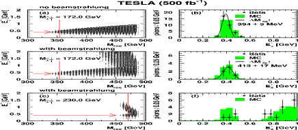
Figure 17: The ISR photon recoil mass and the pion energy scatter plot (left), and the pion energy spectrum across the red line (right) for $e^{+}_{R}e^{-}_{L}\to\tilde{\chi}^{+}_{1}\tilde{\chi}^{-}_{1}\gamma\to\pi^{+}\pi^{-}\gamma E\kern-6.00006pt/$ [58].

Besides the $e^{+}e^{-}$ option, chargino pair production

$$\gamma\gamma\rightarrow\tilde{\chi}^{+}_{i}\tilde{\chi}^{-}_{i}(i=1,2)$$ (17)

in the $\gamma\gamma$ mode of a Linear Collider has been studied [59]. In this case the production is a pure QED process (at tree level) and therefore it allows the chargino decay mechanism to be studied separately in contrast to the $e^{+}e^{-}$ mode where both production and decay are sensitive to the SUSY parameters.

Provided the chargino mass has been measured and the energy spectrum and polarization of the high energy photons are well under control, the production cross section and the polarization of the charginos in reaction eq. (17) are uniquely predicted. By manipulating the polarization of the laser photons and the converted electron beam various characteristics of the chargino decay can be measured and exploited to study the gaugino system. As an example, in [59] the forward-backward asymmetry (measured with respect to the $e^{+}e^{-}$ beam direction)

$$A_{\mathrm{FB}}=\frac{\sigma_{e}(\cos\theta_{e^{+}}>0)-\sigma_{e}(\cos\theta_{e^{+}}<0)}{\sigma_{e}(\cos\theta_{e^{+}}>0)+\sigma_{e}(\cos\theta_{e^{+}}<0)}$$ (18)

of the positron from the decay $\tilde{\chi}_{1}^{+}\to\tilde{\chi}_{1}^{0}e^{+}\nu_{e}$, shown in fig. 18, has been studied to determine $M_{1}$ and $m_{{\tilde{\nu}}_{e}}$.

                        $M_{1}$ [GeV]                             $m_{{\tilde{\nu}}_{e}}$ [GeV]

Figure 18: The $e^{+}$ forward-backward asymmetry (in %) in the ee-CMS of the decay positron from $\gamma\gamma\to\tilde{\chi}^{+}_{1}\tilde{\chi}^{-}_{1}$, $\tilde{\chi}^{+}_{1}\to\tilde{\chi}^{0}_{1}e^{+}\nu_{e}$ as a function of the parameter $M_{1}$ (left) and the sneutrino mass $m_{{\tilde{\nu}}_{e}}$ (right) at $\sqrt{s_{ee}}=500$ GeV for $M_{2}=152$ GeV, $\mu=316$ GeV, $\tan\beta=3$. The shadowed region corresponds to the bound $m_{\tilde{\chi}_{1}^{0}}>38$ GeV [59].

3.2 Neutralinos

Similarly to the chargino case, the di-lepton energy and mass distributions in the reaction $e^{+}e^{-}\to\tilde{\chi}^{0}_{2}\tilde{\chi}^{0}_{2}\to 4\ell^{\pm}E\kern-6.00006pt/$ can be used to determine $\tilde{\chi}^{0}_{1}$ and $\tilde{\chi}^{0}_{2}$ masses. Previous analyses of the di-lepton mass and di-lepton energy spectra performed in the $\tan\beta=3$ case showed that uncertainties in the primary and secondary $\tilde{\chi}^{0}_{2}$ and $\tilde{\chi}^{0}_{1}$ masses of about 2 per mil can be expected [1, 25]. Higher resolution of order 100 MeV for $m_{\tilde{\chi}^{0}_{2}}$ can be obtained from a threshold scan of $e^{+}e^{-}\to\tilde{\chi}^{0}_{2}\tilde{\chi}^{0}_{2}$; heavier states $\tilde{\chi}^{0}_{3}$ and $\tilde{\chi}^{0}_{4}$, if accessible, can still be resolved with a resolution of a few hundred MeV. For the higher values of $\tan\beta\;\raisebox{-3.87495pt}{$\textstyle\stackrel{{\scriptstyle\textstyle>}}{{\sim}}$}\;10$ the dominant decay mode of $\tilde{\chi}^{0}_{2}$ is to $\tau^{+}\tau^{-}\tilde{\chi}^{0}_{1}$. With $\tau$’s decaying in the final state the experimental selection of the signal from the SM and SUSY background becomes more difficult. Preliminary analyses nevertheless show [60] that an accuracy of 1-2 GeV for the mass determination seems possible from the process $e^{+}e^{-}\to\tilde{\chi}^{0}_{1}\tilde{\chi}^{0}_{2}$.

To resolve the light chargino case in the CP-violating scenario (ii) discussed in the previous section, we note that each neutralino mass $m_{\tilde{\chi}^{0}_{i}}$ satisfies the characteristic equation

$$(\Re{\rm e}{M_{1}})^{2}+(\Im{\rm m}{M_{1}})^{2}+u_{i}\,\Re{\rm e}{M_{1}}+v_{i}\,\Im{\rm m}{M_{1}}=w_{i}$$ (19)

where $u_{i},\,v_{i},\,w_{i}$ are functions of $m_{\tilde{\chi}^{0}_{i}},\,M_{2},\,\mu,\,\tan\beta$; since physical masses are CP-even, $v_{i}$ is necessarily proportional to $\sin\varphi_{\mu}$. Therefore each neutralino mass defines a circle in the $\{\Re{\rm e}M_{1},\Im{\rm m}M_{1}\}$ plane, assuming other parameters fixed. With two light neutralino masses two crossing points in the ($\Re{\rm e}{M_{1}}$, $\Im{\rm m}{M_{1}}$) plane are found, fig. 19 (left). Since from the chargino sector $\{M_{2},\mu\;\tan\beta\}$ are parameterized by the unknown $m_{\tilde{\chi}^{\pm}_{2}}$, the crossing points will migrate with $m_{\tilde{\chi}^{\pm}_{2}}$, fig. 19 (right).

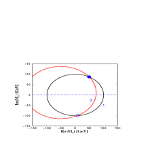
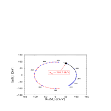
Figure 19: Two crossing points determined by two light neutralinos (left) and their migration with $m_{\tilde{\chi}^{\pm}_{2}}$ (right) [56].

Using the measured cross section for $\tilde{\chi}^{0}_{1}\tilde{\chi}^{0}_{2}$, a unique solution for $M_{1}$ is obtained and the heavy chargino mass predicted. If the LC would run concurrently with the LHC, the LHC experiments might be able to verify the predicted value of $m_{\tilde{\chi}^{\pm}_{2}}$.

3.3 Neutralinos with CP-violating phases

Particularly interesting is the threshold behavior since due to the Majorana nature of neutralinos [52], a clear indication of non–zero CP violating phases can be provided by studying the excitation curve for non–diagonal neutralino pair production near thresholds.

Like in the quark sector, it is useful [52, 61] to represent the unitarity constraints

$$M_{ij}=N_{i1}N^{*}_{j1}+N_{i2}N^{*}_{j2}+N_{i3}N^{*}_{j3}+N_{i4}N^{*}_{j4}\qquad{}$$ (20)

$$D_{ij}=N_{1i}N^{*}_{1j}+N_{2i}N^{*}_{2j}+N_{3i}N^{*}_{3j}+N_{4i}N^{*}_{4j}$$ (21)

on the neutralino mixing matrix $N$, eq. (10), in terms of unitarity quadrangles. For $i$$\neq$$j$ we get $M_{ij}$=$D_{ij}$=0 and the above equations define two types of quadrangles in the complex plane. The $M$-type quadrangles are formed by the sides $N_{ik}N^{*}_{jk}$ connecting two rows $i$ and $j$, eq. (20), and the $D$-type by $N_{ki}N^{*}_{kj}$ connecting two columns $i$ and $j$, eq. (21), of the mixing matrix. By a proper ordering of sides the quadrangles are assumed to be convex with areas

$${\rm area}[M_{ij}]={\textstyle\frac{1}{4}}(|J_{ij}^{12}|+|J_{ij}^{23}|+|J_{ij}^{34}|+|J_{ij}^{41}|)$$ (22)

$${\rm area}[D_{ij}]={\textstyle\frac{1}{4}}(|J_{12}^{ij}|+|J_{23}^{ij}|+|J_{34}^{ij}|+|J_{41}^{ij}|)$$ (23)

where $J_{ij}^{kl}$ are the Jarlskog–type CP–odd “plaquettes” [62]

$$J_{ij}^{kl}=\Im{\rm m}N_{ik}N_{jl}N_{jk}^{*}N_{il}^{*}$$ (24)

Note that plaquettes, and therefore the areas of unitarity quadrangles, are not sensitive to the Majorana phases $\alpha_{i}$. Unlike in the quark or lepton sector, the orientation of all quadrangles is physically meaningful, and determined by the CP-phases of the neutralino mass matrix.

For a CP-conserving case with real $M_{1},M_{2}$ and $\mu$, the neutralino mixing matrix $N$ has all Dirac phases $\beta_{ij}=0$ mod $\pi$ and Majorana phases $\alpha_{i}=0$ mod $\pi/2$. Majorana phases $\alpha_{i}=\pm\pi/2$ describe only different CP parities of the neutralino states. In terms of quadrangles, CP is conserved if and only if all quadrangles have null area (collapse to lines or points) and are oriented along either the real or the imaginary axis.

The non–zero values of CP-odd quantities, like $\Sigma_{n}$ or the polarization of the produced neutralino normal to the production plane, would unambiguously indicate CP-violation in the neutralino sector. In [63] the CP-odd asymmetry defined as

$${\cal A}=\frac{\sigma(T>0)-\sigma(T<0)}{\sigma(T>0)+\sigma(T<0)}$$ (25)

where $T=\vec{p}(e^{-})\times\vec{p}(l_{1})\cdot\vec{p}(l_{2})$ for the process $e^{+}e^{-}\to\tilde{\chi}^{0}_{1}\tilde{\chi}^{0}_{2}\to\tilde{\chi}^{0}_{1}\tilde{\chi}^{0}_{1}l_{1}l_{2}$ with two visible leptons in the final state has been considered. In fig. 20 the expected cross section (left) and the asymmetry (right) are shown as functions of $M_{2}$ and $\mu$ assuming $\varphi_{1}=\pi/2$.

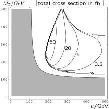
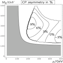
Figure 20: Cross section (left) and CP-odd asymmetry for $e^{+}e^{-}\to\tilde{\chi}^{0}_{1}\tilde{\chi}^{0}_{2}\to\tilde{\chi}^{0}_{1}\tilde{\chi}^{0}_{1}l_{1}l_{2}$ at $\sqrt{s}$=500 GeV with $m_{0}$=100 GeV, $\tan\beta$=10 and gaugino mass universality. In shaded area $m_{\tilde{\chi}^{\pm}_{1}}<$104 GeV [63].

One can also try to identify the presence of CP-phases by studying their impact on CP-even quantities, like neutralino masses, branching ratios etc. Since these quantities are non–zero in the CP-conserving case, the detection of CP-odd phases will require a careful quantitative analysis of a number of physical observables [64], in particular for numerically small CP-odd phases. For example, fig. 21 displays the unitarity quadrangles for the SPS#1a point assuming a small non-vanishing phase $\varphi_{1}=\pi/5$ (consistent with all experimental constraints) [65]. The quadrangles are almost degenerate to lines parallel to either the real or the imaginary axis, and revealing a small phase of $M_{1}$ will be quite difficult.

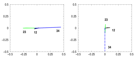
Figure 21: The $D$–type (left panel) and $M$–type (right panel) quadrangles in the complex plane, illustrated for $\tan\beta=10$, $|M_{1}|=100.5$ GeV, $\varphi_{1}=\pi/5$, $M_{2}=190.8$ GeV, $|\mu|=365.1$ GeV and $\varphi_{\mu}=0$; $ij$ as indicated in the figure [65].

However, studying the threshold behavior of the production cross sections can be of great help [52, 65].

If CP is conserved, the CP parity of a pair of Majorana fermions $\tilde{\chi}^{0}_{i}\tilde{\chi}^{0}_{j}$ produced in the static limit in $e^{+}e^{-}$ collisions by a spin-1 current with positive intrinsic CP must satisfy the relation

$$\eta^{i}\eta^{j}(-1)^{L}=1$$ (26)

where $\eta^{i}=\pm i$ is the intrinsic CP parity of $\tilde{\chi}^{0}_{i}$ and $L$ is the angular momentum [66]. Therefore neutralinos with the same CP parities (for example $i=j$) can only be excited in P-wave. The S-wave excitation, with the characteristic steep rise $\sim\beta$ of the cross section near threshold, can occur only for $i\neq j$ with opposite CP–parities of the produced neutralinos [67]. This immediately implies that if the $\{ij\}$ and $\{ik\}$ pairs are excited in the S–wave, the pair $\{jk\}$ must be excited in the P–wave characterized by the slow rise $\beta^{3}$ of the cross section, fig. 22, left panel.

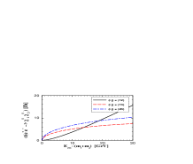
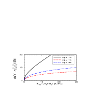
Figure 22: The threshold behavior of the neutralino production cross–sections $\sigma^{\{ij\}}$ for the CP–conserving (left panel) and the CP–violating (right panel) cases. Other parameters as in fig. 21 [65].

If CP is violated, however, the angular momentum of the produced neutralino pair is no longer restricted by the eq. (26) and all non–diagonal pairs can be excited in the S–wave. This is illustrated in fig. 22, where the threshold behavior of the neutralino pairs $\{12\}$, $\{13\}$ and $\{23\}$ for the CP-conserving (left panel) case is contrasted to the CP-violating case (right panel). Even for a small CP–phase $\varphi_{1}=\pi/5$, virtually invisible in the shape and orientation of unitarity quadrangles in fig. 21, the change in the energy dependence near threshold can be quite dramatic. Thus, observing the $\{ij\}$, $\{ik\}$ and $\{jk\}$ pairs to be excited all in S–wave states would therefore signal CP–violation.

3.4 Gluinos

Strongly interacting gluinos will copiously be produced at the LHC. Only for rather light gluinos, $m_{\tilde{g}}\sim$ 200 – 300 GeV, can a 1 TeV LC improve on the LHC gluino mass measurement.

In $e^{+}e^{-}$ annihilation the exclusive production of gluino pairs proceeds only at the loop level: $s$-channel photons and $Z^{0}$ bosons couple to the gluinos via triangular quark and squark loops. Moreover, near threshold the pairs of identical Majorana gluinos are excited in a P-wave with a slow rise of the cross section. As a result, the production cross sections are rather small even for relatively light gluinos, see left panel of fig. 23. For $m_{\tilde{g}}\;\raisebox{-3.87495pt}{$\textstyle\stackrel{{\scriptstyle\textstyle>}}{{\sim}}$}\;500$ GeV, no events at LC with luminosities of 1 ab^-1 per year are expected irrespectively of their collision energy.

In the $\gamma\gamma$ option, the chances to observe gluinos are better. First, the gluino pairs can be excited in an S-wave with a faster rise of the cross section. Second, for $m_{\tilde{q}}\gg m_{\tilde{g}}$ the production can be enhanced by resolved photons. As seen in the right panel of fig. 23, the production cross sections in the polarized $e^{-}e^{-}$ option can reach several fb in a wider range of gluino masses.

Figure 23: Gluino production cross section in $e^{+}e^{-}$ annihilation (left), and in polarized direct photon collisions generated in $e^{-}e^{-}$ (right). [68].

4 R–parity violating SUSY

In the MSSM the multiplicative quantum number R–parity is conserved. Under this symmetry all standard model particles have $R_{p}=+1$ and their superpartners $R_{p}=-1$. As a result, the lightest SUSY particle (LSP) is stable, SUSY particles are only produced in pairs with the distinct signature of missing energy in an experiment. However, R–parity conservation has no strong theoretical justification since the superpotential admits explicit R–parity violating ($/{R}_{p}$) terms

$$W_{/{R}_{p}}=\epsilon_{i}L_{i}H_{u}+{\textstyle\frac{1}{2}}\lambda_{ijk}L_{i}L_{j}\bar{D}_{k}$$

$$~{}~{}~{}~{}~{}~{}~{}~{}~{}+\lambda^{\prime}_{ijk}L_{i}Q_{j}\bar{D}_{k}+{\textstyle\frac{1}{2}}\lambda^{\prime\prime}_{ijk}\bar{U}_{i}\bar{D}_{j}\bar{D}_{k}$$ (27)

where $H_{u},L,Q$ are the Higgs and left–handed lepton and squark superfields, and $\bar{E},\bar{D},\bar{U}$ are the corresponding right–handed fields. R–parity violation changes the SUSY phenomenology drastically. The LSP decays, so the characteristic signature of missing energy in the $/{R}_{p}$ conserving MSSM is replaced by multi–lepton and/or multi–jet final states.

The couplings $\epsilon$, $\lambda$ and $\lambda^{\prime}$ violate lepton number, while $\lambda^{\prime\prime}$ violate baryon number. If both types of couplings were present, they would induce fast proton decay. This can be avoided by assuming at most one type of couplings to be non-vanishing.

4.1 Bilinear R–parity violation

Models with explicit bilinear breaking of R–parity (BRpV) assume only $\epsilon_{i}\neq 0$ in eq. (27) and the corresponding terms in the soft SUSY breaking part of the Lagrangian ${\cal L}_{soft}\ni B_{i}\epsilon_{i}{\tilde{L}}_{i}H_{u}$ [69]. As a result, the sneutrinos develop non-zero vacuum expectation $v_{i}=\langle{\tilde{\nu}}_{i}\rangle$ in addition to the VEVs $v_{u}$ and $v_{d}$ of the MSSM Higgs fields $H_{u}^{0}$ and $H_{d}^{0}$. The bilinear parameters $\epsilon_{i}$ and $v_{i}$ induce mixing between particles that differ only by R–parity: charged leptons mix with charginos, neutrinos with neutralinos, and Higgs bosons with sleptons. Mixing between the neutrinos and the neutralinos generates at tree level a non-zero mass $m_{\nu_{3}}\sim M_{2}|\vec{\Lambda}|^{2}/{\rm Det}(M_{\tilde{\chi}^{0}})$ (where $\Lambda_{i}=\epsilon_{i}v_{d}+\mu v_{i}$) for one of the three neutrinos and the mixing angle $\tan^{2}\theta_{atm}\sim(\Lambda_{2}/\Lambda_{3})^{2}$; the remaining two masses and mixing angles are generated at 1-loop. For example, the solar mixing angle scales as $\tan^{2}\theta_{sol}\sim(\epsilon_{1}/\epsilon_{2})^{2}$. Thus the model can provide a simple and calculable framework for neutrino masses and mixing angles in agreement with the experimental data, and at the same time leads to clear predictions for the collider physics [70].

$\tan^{2}\theta_{atm}$                          $\tan^{2}\theta_{sol}$

Figure 24: Left: BR($\tilde{\chi}^{+}_{1}$$\to$$\mu^{+}q\bar{q}$)/BR($\tilde{\chi}^{+}_{1}$$\to$$\tau^{+}q\bar{q}$) as a function of $\tan^{2}\theta_{atm}$. Right: BR(${\tilde{b}}_{1}$$\to$$e^{+}t$)/BR(${\tilde{b}}_{1}$$\to$$\mu^{+}t$) as a function of $\tan^{2}\theta_{sol}$ [71].

For small $/{R}_{p}$ couplings, production and decays of SUSY particles is as in the MSSM except that the LSP decays. Since the astrophysical constraints on the LSP no longer apply, a priori any SUSY particle could be the LSP. In a recent study [71] a sample of the SUSY parameter space with $/{R}_{p}$ couplings consistent with neutrino masses shows that irrespectively of the LSP nature, there is always at least one correlation between ratios of LSP decay branching ratios and one of the neutrino mixing angles. Two examples of chargino and squark being the LSP are shown in fig. 24.

4.2 Bilinear versus Trilinear $/{R}_{p}$

In the case of charged slepton LSP, the collider physics might distinguish whether bilinear or trilinear couplings are dominant sources of $/{R}_{p}$ and the neutrino mass matrix [72]. Possible final states of the LSP are either $l_{j}\nu_{k}$ or $q{\bar{q}}^{\prime}$. If the LSP is dominantly right-chiral, the former by far dominate over the hadronic decay mode. In the case of TRpV, the two-body decay width for ${\tilde{l}}_{i}\rightarrow l_{j}+\Sigma_{k}\nu_{k}$ scales as $\Gamma\sim\Sigma_{k}\sin^{2}\theta_{\tilde{l}_{i}}\lambda^{2}_{kji}$ provided $\lambda^{\prime}\;\raisebox{-3.87495pt}{$\textstyle\stackrel{{\scriptstyle\textstyle<}}{{\sim}}$}\;\lambda$, while for the BRpV one has $\Gamma\sim Y_{i}\sin^{2}\theta_{\tilde{l}_{i}}\epsilon^{2}_{j}$ for $i\neq j$ ($Y_{i}$ is the corresponding Yukawa coupling), and BR$({\tilde{e}}_{1}\rightarrow e\Sigma_{k}\nu_{k})\sim 1$. Immediately one finds then

$${\rm BR}({\tilde{e}}_{1}\rightarrow e\Sigma_{k}\nu_{k})=\left\{\begin{array}[]{l}\sim 1~{}~{}~{}~{}~{}~{}~{}~{}{\rm for~{}BRpV}\\ \;\raisebox{-3.87495pt}{$\textstyle\stackrel{{\scriptstyle\textstyle<}}{{\sim}}$}\;0.5~{}~{}~{}~{}{\rm for~{}TRpV}\end{array}\right.$$ (30)

Therefore, the LC measurements of the ${\tilde{l}}_{i}$ decay modes can distinguish between bilinear or trilinear terms as dominant contributions to the neutrino masses [72].

For trilinear couplings of the order of current experimental upper bounds, in particular for the third generation (s)fermions, additional production as well as decay channels may produce strikingly new signatures. For example, sneutrinos could be produced as an s-channel resonance in $e^{+}e^{-}$ annihilation. During this workshop single sneutrino production in association with fermion pairs at polarised photon colliders has been analysed [73]. The associate mode may also appear with fermions of different flavour [74], so that the signal is basically SM background free. Moreover, the advantage of exploiting $\gamma\gamma$ collisions in place of $e^{+}e^{-}$ ones in producing single sneutrinos with a fermion pair of differnt flavour resides in the fact that the cross sections for the former are generally larger than those for the latter. As an example, fig. 25 shows the unpolarised production rates for both the $\gamma\gamma$ and $e^{+}e^{-}$ induced ${\tilde{\nu}}\tau^{\pm}\mu^{\mp}$ modes at $\sqrt{s_{e^{+}e^{-}}}=500$ GeV and 1 TeV. For illustration, the couplings are set $\lambda=\lambda^{\prime}=1$.

Figure 25: $\sigma({\tilde{\nu}}\tau^{\pm}\mu^{\mp})$ at $\gamma\gamma$ (a,b) and $e^{+}e^{-}$ (c,d) collider with $\sqrt{s}$=100 GeV (a,c) and 1 TeV (b,d) [73].                      

5 Extended SUSY

The NMSSM, the minimal extension of the MSSM, introduces a singlet superfield field $S$ in the superpotential

$$W\supset\lambda H_{u}H_{d}S-\frac{1}{3}\kappa S^{3}\,.$$ (31)

In this model, an effective $\mu=\lambda x$ term is generated when the scalar component of the singlet $S$ acquires a vacuum expectation value $x=\langle S\rangle$. The fermion component of the singlet superfield (singlino) will mix with neutral gauginos and higgsinos after electroweak gauge symmetry breaking, changing the neutralino mass matrix to the 5$\times$5 form which depends on $M_{1}$, $M_{2}$, $\tan\beta$, $x$ and the trilinear couplings $\lambda$ and $\kappa$.

In some regions of the parameter space the singlino may be the lightest supersymmetric particle, weakly mixing with other states. In the extended SPS#1a scenario with large $x\gg|M_{2}|$, analysed in [75], the lightest neutralino $\tilde{\chi}^{0}_{S}$ with mass $\approx 2\kappa x$ becomes singlino-dominated while the other four neutralinos $\tilde{\chi}^{0}_{1,\ldots,4}$ have the MSSM characteristics. The exotic $\tilde{\chi}^{0}_{S}$ state can be searched for in the associated production of $\tilde{\chi}^{0}_{S}$ together with the lightest MSSM-like neutralino $\tilde{\chi}^{0}_{1}$ in $e^{+}e^{-}$ annihilation. The unpolarized cross section, shown in fig. 26 for $m_{\tilde{\chi}^{0}_{S}}=70$ GeV, is larger than 1 fb up to $x<7.4$ TeV which corresponds to a singlino content of 99.7 %. Polarized beams can enhance the cross section by a factor 2–3, and provide discriminating power between different scenarios [76]. If the couplings of a singlino-dominated LSP to the NLSP are strongly suppressed at large values of $x$, displaced vertices in the NMSSM may be generated, fig. 26, which would clearly signal the extension of the minimal model. For a similar analysis in the E₆ inspired model we refer to [75].

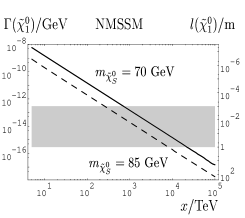
Figure 26: Left: Unpolarized $\sigma(\tilde{\chi}^{0}_{S}\tilde{\chi}^{0}_{1}$) at $\sqrt{s}$=500 GeV (solid) and for polarized beams ${\cal P}_{-}$=0.8, ${\cal P}_{+}$=-0.6 (dashed), ${\cal P}_{-}$=-0.8, ${\cal P}_{+}$=0.6 (dotted). Right: Total decay widths of the lightest MSSM-like $\tilde{\chi}^{0}_{1}$ decaying into a singlino-dominated $\tilde{\chi}^{0}_{S}$. The shaded area shows where displaced vertices exist [75].

However, if the spectrum of the four lighter neutralinos in the extended model is similar to the spectrum in the MSSM, but the mixing is substantial, discriminating the models by analysing the mass spectrum becomes very difficult. Studying in this case the summed-up cross sections of the four light neutralinos may then be a crucial method to reveal the structure of the neutralino system [52]. More specifically, in extended SUSY models with $n$ SU(2) doublet and $m$ SU(2) singlet chiral superfields, the sum rule reads

$$\lim_{s\rightarrow\infty}\,s\,{\textstyle\sum_{i\leq j}}\;\sigma\{ij\}={\textstyle\frac{\pi\alpha^{2}}{48\,c^{4}_{W}s^{4}_{W}}}$$

$$~{}~{}~{}~{}\times\left[\,n\,(8s^{4}_{W}-4s^{2}_{W}+1)\,+48s^{4}_{W}+3\right]$$ (32)

The right–hand side of eq. (32) is independent of the number $m$ of singlets and it reduces to the sum rule in the MSSM for $n=2$. In fig. 27 the exact sum rules, normalized to the asymptotic value, are compared for an NMSSM scenario giving rise to one very heavy neutralino with $m_{\tilde{\chi}^{0}_{5}}\sim 1000$ GeV, and to four lighter neutralinos with masses equal within 2 – 5 GeV to the neutralino masses in the MSSM. Due to the incompleteness of these states below the thresholds for producing the heavy neutralino $\tilde{\chi}^{0}_{5}$, the NMSSM value differs significantly from the corresponding sum rule of the MSSM. Therefore, even if the extended neutralino states are very heavy, the study of sum rules can shed light on the underlying structure of the supersymmetric model.

Figure 27: The sum of neutralino–pair production cross sections: all pairs in the MSSM (solid), and of the first four neutralino states in the NMSSM (dashed); both normalized to the asymptotic value [52].

6 Reconstructing fundamental SUSY parameters

Low energy SUSY particle physics is characterized by energy scales of order  $\textstyle\stackrel{{\scriptstyle\textstyle<}}{{\sim}}$  1 TeV. However, the roots for all the phenomena we will observe experimentally in this range may go to energies near the Planck or the GUT scale. Fortunately, supersymmetry provides us with a stable bridge between these two vastly different energy regions [77]. To this purpose renormalization group equations (RGE) are exploited, by which parameters from low to high scales are evolved based on nothing but measured quantities in laboratory experiments. This procedure has very successfully been pursued for the three electroweak and strong gauge couplings, and has been expanded to a large ensemble of supersymmetry parameters [78] – the soft SUSY breaking parameters: gaugino and scalar masses, as well as trilinear couplings. This bottom-up approach makes use of the low-energy measurements to the maximum extent possible and it reveals the quality with which the fundamental theory at the high scale can be reconstructed in a transparent way.

A set of representative examples in this context has been studied [79]: minimal supergravity and a left–right symmetric extension; gauge mediated supersymmetry breaking; and superstring effective field theories. The anomaly mediated as well as the gaugino mediated SUSY breaking are technically equivalent to the mSUGRA case and therefore were not treated explicitly.

6.1 Gravity mediated SUSY breaking

The minimal supergravity scenario mSUGRA is characterized by the universal: gaugino mass $M_{1/2}$, scalar mass $M_{0}$, trilinear coupling $A_{0}$, sign of $\mu$ (the modulus $|\mu|$ determined by radiative symmetry breaking) and $\tan\beta$. The parameters $M_{1/2}$, $M_{0}$ and $A_{0}$ are defined at the GUT scale $M_{U}$ where gauge couplings unify $\alpha_{i}=\alpha_{U}$. The RGE are then used to determine the low energy SUSY lagrangian parameters.

The point chosen for the analysis is close to the Snowmass Point SPS#1a [8], except for the scalar mass parameter $M_{0}$ which was taken slightly larger for merely illustrative purpose: $M_{1/2}=250$ GeV, $M_{0}=200$ GeV, $A_{0}=-100$ GeV, $\tan\beta=10$ and $sign(\mu)=+$.

Table 1: Representative gaugino/scalar mass parameters and couplings as determined at the electroweak scale and evolved to the GUT scale in the mSUGRA scenario based on LHC and LC simulations; masses are in GeV. The errors are 1$\sigma$ [79].

	Exp. Input	GUT Value
$M_{1}$	102.31 $\pm$ 0.25	$250.00\pm 0.33$
$M_{2}$	192.24 $\pm$ 0.48	$250.00\pm 0.52$
$M_{3}$	586 $\pm$ 12	$250.0\pm 5.3$
$\mu$	358.23 $\pm$ 0.28	$355.6\pm 1.2$
$M^{2}_{L_{1}}$	$(6.768\pm 0.005)\cdot 10^{4}$	$(3.99\pm 0.41)\cdot 10^{4}$
$M^{2}_{E_{1}}$	$(4.835\pm 0.007)\cdot 10^{4}$	$(4.02\pm 0.82)\cdot 10^{4}$
$M^{2}_{Q_{1}}$	$(3.27\pm 0.08)\cdot 10^{5}$	$(3.9\pm 1.5)\cdot 10^{4}$
$M^{2}_{U_{1}}$	$(3.05\pm 0.11)\cdot 10^{5}$	$(3.9\pm 1.9)\cdot 10^{4}$
$M^{2}_{D_{1}}$	$(3.05\pm 0.11)\cdot 10^{5}$	$(4.0\pm 1.9)\cdot 10^{4}$
$M^{2}_{H_{1}}$	$(6.21\pm 0.08)\cdot 10^{4}$	$(4.01\pm 0.54)\cdot 10^{4}$
$M^{2}_{H_{2}}$	$(-1.298\pm 0.004)\cdot 10^{5}$	$(4.1\pm 3.2)\cdot 10^{4}$
$A_{tit}$	$-446\pm 14$	$-100\pm 54$
$\tan\beta$	$9.9\pm 0.9$	—

Based on simulations and estimates of expected precision, the low-energy ’experimental’ values are taken as the input values for the evolution of the mass parameters in the bottom-up approach to the GUT scale. The results for the evolution of the mass parameters to the GUT scale $M_{U}$ are shown in fig. 28. The left panel presents the evolution of the gaugino parameters $M_{i}^{-1}$, while the right panel shows the extrapolation of the slepton mass parameters squared of the first two generations. The accuracy deteriorates for the squark mass parameters and for the Higgs mass parameter $M^{2}_{H_{2}}$. The origin of the differences between the errors for slepton, squark and Higgs mass parameters can be traced back to the numerical size of the coefficients. The quality of the test is apparent from table 1, where it is shown how well the reconstructed mass parameters at the GUT scale reproduce the input values $M_{1/2}=250$ GeV and $M_{0}=200$ GeV.

$1/M_{i}$ [GeV${}^{-1}]$                           $M^{2}_{\tilde{j}}$ [$10^{3}$ GeV²]
$Q$ [GeV]                              $Q$ [GeV]

Figure 28: mSUGRA: Evolution, from low to high scales, of gaugino mass parameters (left), and first two generation sfermion mass parameters and the Higgs mass parameter $M^{2}_{H_{2}}$ (right). The widths of the bands indicate the 1$\sigma$ CL [79].

The above analysis has also been extended [79] to a left–right supersymmetric $SO(10)$ model in which the $SO(10)$ symmetry is assumed to be realized at a scale between the standard $SU(5)$ scale $M_{U}\simeq 2\cdot 10^{16}$, derived from the unification of the gauge couplings, and the Planck scale $M_{P}\simeq 10^{19}$ GeV. The right–handed neutrinos are assumed heavy, with masses at intermediate scales between $O(10^{10})$ GeV and $O(10^{15})$ GeV, so that the observed light neutrino masses are generated by the see-saw mechanism. The evolution of the gaugino and scalar mass parameters of the first two generations is not affected by the left–right extension. It is only different for the third generation and for $M^{2}_{H_{2}}$ owing to the enhanced Yukawa coupling in this case. The sensitivity to the intermediate $\nu_{R}$ scales is rather weak because neutrino Yukawa couplings affect the evolution of the sfermion mass parameters only mildly. Nevertheless, a rough estimate of the intermediate scale follows from the evolution of the mass parameters to the low experimental scale if universality holds at the Grand Unification scale.

6.2 Gauge mediated SUSY breaking

In GMSB the scalar and the F components of a Standard–Model singlet superfield $S$ acquire vacuum expectation values $\langle S\rangle$ and $\langle F_{S}\rangle$ through interactions with fields in the secluded sector, thus breaking supersymmetry. Vector-like messenger fields $M$, carrying non–zero $SU(3)\times SU(2)\times U(1)$ charges and coupling to $S$, transport the supersymmetry breaking to the eigen–world. The system is characterized by the mass $M_{M}\sim$ $\langle S\rangle$ of the messenger fields and the mass scale $\Lambda={\langle F_{S}\rangle}/{\langle S\rangle}$ setting the size of the gaugino and scalar masses. $M_{M}$ is expected to be in the range of 10 to $10^{6}$ TeV and $\Lambda$ has to be smaller than $M_{M}$.

The gaugino masses are generated by loops of scalar and fermionic messenger component fields, while masses of the scalar fields in the visible sector are generated by 2-loop effects of gauge/gaugino and messenger fields, and the $A$ parameters are generated at 3-loop level and they are practically zero at $M_{M}$. Scalar particles with identical Standard–Model charges squared have equal masses at the messenger scale $M_{M}$, which is a characterictic feature of the GMSB model.

This scheme has been investigated for the point $\Lambda=100$ TeV, $M_{M}=200$ TeV, $N_{5}=1$, $N_{10}=0$, $\tan\beta=15$ and $\mu>0$ corresponding to the Snowmass Point SPS#8. The evolution of the gaugino and sfermion mass parameters of the first two generations as well as the Higgs mass parameters, including 2-loop $\beta$–functions, is presented in fig. 29.

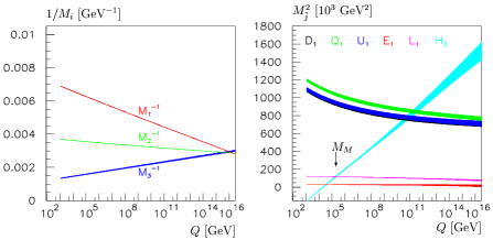
Figure 29: GMSB: Evolution, from low to high scales, of gaugino mass parameters (left), and first two generation sfermion mass parameters and the Higgs mass parameter $M^{2}_{H_{2}}$ (right). The widths of the bands indicate the 1$\sigma$ CL [79].

The gaugino masses in GMSB evolve nearly in the same way as in mSUGRA. However, due to the influence of the $A$–parameters in the 2-loop RGEs for the gaugino mass parameters, they do not meet at the same point as the gauge couplings in this scheme. On the other hand the running of the scalar masses is quite different in both theories. The bands of the slepton $L$–doublet mass parameter $M^{2}_{\tilde{L}}$ and the Higgs parameter $M^{2}_{H_{2}}$, which carry the same moduli of standard–model charges, cross at the scale $M_{M}$. The crossing, indicated by an arrow in the fig. 29, is a necessary condition (in the minimal form) for the GMSB scenario to be realized. Moreover, at the messenger scale the ratios of scalar masses squared in the simplest version of GMSB are determined solely by group factors and gauge couplings, being independent of the specific GMSB characteristics, i. e. messenger multiplicities and $\Lambda$ mass scale.

The two scales $\Lambda$ and $M_{M}$, and the messenger multiplicity $N_{M}=N_{5}+3N_{10}$ can be extracted from the spectrum of the gaugino and scalar particles. For the point analyzed in the example above, the following accuracy for the mass parameters and the messenger multiplicity has been found:

$$\Lambda = (1.01\pm 0.03)\cdot 10^{2}\;\rm{TeV}$$ (33)

$$M_{M} = (1.92\pm 0.24)\cdot 10^{2}\;\rm{TeV}$$ (34)

$$N_{M} = 0.978\pm 0.056$$ (35)

6.3 String induced SUSY breaking

Four–dimensional strings naturally give rise to a minimal set of fields for inducing supersymmetry breaking; they play the rôle of the fields in the hidden sectors: the dilaton $S$ and the moduli $T_{m}$ chiral superfields which are generically present in large classes of 4–dimensional heterotic string theories. In the analysis only one moduli field $T$ has been considered. SUSY breaking, mediated by a goldstino field, originates in the vacuum expectation values of $S$ and $T$ generated by genuinely non–perturbative effects. The properties of the model depend on the composition of the goldstino which is a mixture of the dilaton field $S$ and the moduli field $T$,

$$\tilde{G} = {S}\,\sin\theta+{T}\,\cos\theta$$ (36)

Universality is generally broken in such a scenario by a set of non-universal modular weights $n_{j}$ that determine the coupling of $T$ to the SUSY matter fields $\Phi_{j}$. The gaugino and scalar mass parameters can be expressed to leading order by the gravitino mass $m_{3/2}$, the vacuum values $\langle S\rangle$ and $\langle T\rangle$, the mixing parameter $\sin\theta$, the modular weights $n_{j}$ and the Green-Schwarz parameter $\delta_{\rm GS}$. The relations between the universal gauge coupling $\alpha(M_{\rm string})$ at the string scale $M_{\rm string}$ and the gauge couplings $\alpha_{i}(M_{\rm GUT})$ at the SU(5) unification scale $M_{\rm GUT}$:

$$\alpha^{-1}_{i}(\rm M_{\rm GUT})=\alpha^{-1}({\rm M_{\rm string}})+\Delta\alpha^{-1}_{i}[n_{j}]$$ (37)

receive small deviations from universality at the GUT scale which are accounted for by string loop effects transporting the couplings from the universal string scale to the GUT scale. The gauge coupling at $M_{\rm string}$ is related to the dilaton field, $g_{s}^{2}=1/{\langle S\rangle}$.

A mixed dilaton/moduli superstring scenario with dominating dilaton field component and with different couplings of the moduli field to the (L,R) sleptons, the (L,R) squarks and to the Higgs fields, corresponding to O–I representation has been chosen for the analysis [79], for which $\sin^{2}\theta=0.9$, $n_{L_{i}}=-3$, $n_{E_{i}}=-1$, $n_{H_{1}}=n_{H_{2}}=-1$, $n_{Q_{i}}=0$, $n_{D_{i}}=1$, $n_{U_{i}}=-2$, and the gravitino mass 180 GeV.

The evolution of the gaugino and scalar mass parameters is displayed in fig. 30. The pattern of the trajectories is remarkably different from other scenarios. The breaking of universality in the gaugino sector, induced by string threshold corrections, is shown in the insert.

$1/M_{i}$ [GeV${}^{-1}]\times 10^{-2}$                   $M^{2}_{\tilde{j}}$ [$10^{3}$ GeV²]
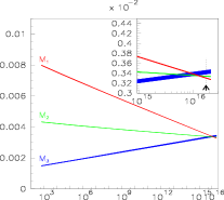
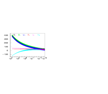
$Q$ [GeV]                              $Q$ [GeV]

Figure 30: String scenario: Evolution, from low to high scales, of gaugino mass parameters (left), and first two generation sfermion mass parameters and the Higgs mass parameter $M^{2}_{H_{2}}$ (right). The widths of the bands indicate the 1$\sigma$ CL [79].

Table 2: Comparison of the experimentally reconstructed values with the ideal fundamental parameters in a specific example for a string effective field theory. [All mass parameters are in units of GeV.]

Parameter	Ideal	Reconstructed
$m_{3/2}$	180	179.9 $\pm$ 0.4
$\langle S\rangle$	2	1.998 $\pm$ 0.006
$\langle T\rangle$	14	14.6 $\pm$ 0.2
$\sin^{2}\theta$	0.9	0.899 $\pm$ 0.002
$g_{s}^{2}$	0.5	0.501 $\pm$ 0.002
$\delta_{GS}$	0	0.1 $\pm$ 0.4
$\tan\beta$	10	10.00 $\pm$ 0.13

The reconstructed values the fundamental parameters of the string effective field theory are compared with the ideal values in Table 2. Also the reproduction of moduli weights as ’integers’ at the per-cent level provides a highly non-trivial check of the string model [79].

7 Summary

Much progress has been achieved during the Extended ECFA/DESY Workshop. It has been demonstrated that a high luminosity LC with polarized beams, and with additional $e\gamma$, $\gamma\gamma$ and $e^{-}e^{-}$ modes, can provide high quality data for the precise determination of low-energy SUSY Lagrangian parameters. In the bottom–up approach, through the evolution of the parameters from the electroweak scale, the regularities in different scenarios at the high scales can be unravelled if precision analyses of the supersymmetric particle sector at $e^{+}e^{-}$ linear colliders are combined with analyses at the LHC. In this way the basis of the SUSY breaking mechanism can be explored and the crucial elements of the fundamental supersymmetric theory can be reconstructed.

So far most analyses were based on lowest–order expressions. With higher order corrections now available, one of the goals of the SUSY WG in the new ECFA Study would be to refine the above program. Many new theoretical calculations and future experimental analyses will be necessary. However, the prospect of exploring elements of the ultimate unification of the interactions provides a strong stimulus in this direction.

References

- [1] J. A. Aguilar-Saavedra et al. [ECFA/DESY LC Physics Working Group Collaboration], “TESLA Technical Design Report Part III: Physics at an e+e- Linear Collider,” arXiv:hep-ph/0106315.
- [2] Understanding Matter, Energy, Space and Time: The Case for the Linear Collider, http://sbhepnt.physics.sunysb. edu/ grannis/ilcsc/lc-icfa-v6.3.pdf
- [3] F. E. Paige, arXiv:hep-ph/0211017. J. G. Branson, D. Denegri, I. Hinchliffe, F. Gianotti, F. E. Paige and P. Sphicas (eds.) [ATLAS and CMS Collaborations], Eur. Phys. J. directC 4 (2002) N1.
- [4] J. Kalinowski, arXiv:hep-ph/0212388.
- [5] G. Weiglein, talk in Amsterdam. The web address of the LHC/LC Study Group: http://www.ippp.dur.ac.uk/ georg/lhclc/.
-
[6]
The web addresses of the
Extended ECFA-DESY meetings:
Cracow http://fatcat.ifj.edu.pl/ecfadesy-krakow/
St. Malo http://www-dapnia.cea.fr/ecfadesy-stmalo/
Prague http://www-hep2.fzu.cz/ecfadesy/Talks/SUSY/
Amsterdam http://www.nikhef.nl/ecfa-desy/start.html - [7] G. Moortgat-Pick, talk in Amsterdam. The web address of the POWER Study Group: http://www.ippp.dur.ac.uk/ gudrid/power/.
- [8] B. C. Allanach et al., in Proc. of the APS/DPF/DPB Summer Study on the Future of Particle Physics (Snowmass 2001) ed. N. Graf; Eur. Phys. J. C 25 (2002) 113 [eConf C010630 (2001) P125] [arXiv:hep-ph/0202233] LC-TH-2003-022. The values of benchmarks are listed on http://www.ippp.dur.ac.uk/ georg/sps
- [9] H. Baer, F. E. Paige, S. D. Protopopescu and X. Tata, arXiv:hep-ph/0001086.
- [10] N. Ghodbane and H. U. Martyn, in Proc. of the APS/DPF/DPB Summer Study on the Future of Particle Physics (Snowmass 2001) ed. N. Graf, arXiv:hep-ph/0201233, LC-PHSM-2003-055, LC-TH-2001-079. B. Allanach, S. Kraml and W. Porod, arXiv:hep-ph/0207314.
- [11] B. C. Allanach, S. Kraml and W. Porod, JHEP 0303 (2003) 016 [arXiv:hep-ph/0302102] LC-TH-2003-017.
- [12] B. C. Allanach, Comput. Phys. Commun. 143 (2002) 305 [arXiv:hep-ph/0104145].
- [13] W. Porod, Comput. Phys. Commun. 153 (2003) 275 [arXiv:hep-ph/0301101] LC-TOOL-2003-042.
- [14] A. Djouadi, J. L. Kneur and G. Moultaka, arXiv:hep-ph/0211331.
- [15] S. Katsanevas and P. Morawitz, Comput. Phys. Commun. 112 (1998) 227 [arXiv:hep-ph/9711417].
- [16] T. Sjostrand, L. Lonnblad and S. Mrenna, arXiv:hep-ph/0108264.
- [17] M. Battaglia et al., in Proc. of the APS/DPF/DPB Summer Study on the Future of Particle Physics (Snowmass 2001) ed. N. Graf, eConf C010630 (2001) P347 [arXiv:hep-ph/0112013].
- [18] A. Bartl et al. [ECFA/DESY SUSY Collaboration], arXiv:hep-ph/0301027, LC-TH-2003-039. A. Freitas et al., [ECFA/DESY SUSY Collaboration], arXiv:hep-ph/0211108. LC-PHSM-2003-019.
- [19] W. Majerotto, arXiv:hep-ph/0209137.
- [20] A. Freitas, D. J. Miller and P. M. Zerwas, Eur. Phys. J. C 21 (2001) 361 [arXiv:hep-ph/0106198] LC-TH-2001-011. A. Freitas and D. J. Miller, in Proc. of the APS/DPF/DPB Summer Study on the Future of Particle Physics (Snowmass 2001) eds. R. Davidson and C. Quigg, [hep-ph/0111430]. A. Freitas and A. von Manteuffel, arXiv:hep-ph/0211105.
- [21] J. Guasch, W. Hollik and J. Sola, JHEP 0210 (2002) 040 [arXiv:hep-ph/0207364]. J. Guasch, W. Hollik and J. Sola, arXiv:hep-ph/0307011, LC-TH-2003-033. W. Hollik and H. Rzehak, arXiv:hep-ph/0305328.
- [22] M. Beccaria, F. M. Renard and C. Verzegnassi, arXiv:hep-ph/0203254, LC-TH-2002-005. M. Beccaria, M. Melles, F. M. Renard and C. Verzegnassi, arXiv:hep-ph/0210283.
- [23] H.U. Martyn, LC-PHSM-2003-07, and talk in Prague.
- [24] H. Nieto-Chaupis, LC-DET-2003-074, and talk in Amsterdam.
- [25] H.U. Martyn, arXiv:hep-ph/0302024.
- [26] M. Dima et al., Phys. Rev. D 65 (2002) 071701.
- [27] E. Boos, G. Moortgat-Pick, H. U. Martyn, M. Sachwitz and A. Vologdin, arXiv:hep-ph/0211040. E. Boos, H.U. Martyn, G. Moortgat-Pick, M. Sachwitz, A. Sherstnev and P.M. Zerwas, arXiv:hep-ph/0303110, LC-PHSM-2003-018.
- [28] M.M. Nojiri, Phys. Rev. D 51 (1995) 6281 [arXiv:hep-ph/9412374]. M.M. Nojiri, K. Fujii and T. Tsukamoto, Phys. Rev. D 54 (1996) 6756 [arXiv:hep-ph/9606370].
- [29] A. Finch, H. Nowak and A. Sopczak, arXiv:hep-ph/0211140, LC-PHSM-2003-075.
- [30] S. Heinemeyer, S. Kraml, W. Porod and G. Weiglein, arXiv:hep-ph/0306181, LC-TH-2003-052.
- [31] C. Blöchinger, H. Fraas, G. Moortgat-Pick and W. Porod, Eur. Phys. J. C 24 (2002) 297 [arXiv:hep-ph/0201282] LC-TH-2003-031.
- [32] A. Freitas, DESY-THESIS-2002-023, A. Freitas, A. von Manteuffel, in [20], A. Freitas, A. von Manteuffel, P.M. Zerwas, in preparation.
- [33] A. Brandenburg, M. Maniatis and M. M. Weber, arXiv:hep-ph/0207278. M. Maniatis, DESY-THESIS-2002-007
- [34] H. Baer, C. Balazs, S. Hesselbach, J. K. Mizukoshi and X. Tata, Phys. Rev. D 63 (2001) 095008 [arXiv:hep-ph/0012205].
- [35] A. Bartl, W. Majerotto, W. Porod and D. Wyler, arXiv:hep-ph/0306050.
- [36] D. Chang, W. Y. Keung and A. Pilaftsis, Phys. Rev. Lett. 82 (1999) 900 [Erratum-ibid. 83 (1999) 3972] [arXiv:hep-ph/9811202]. A. Pilaftsis, Phys. Lett. B 471 (1999) 174 [arXiv:hep-ph/9909485].
- [37] A. Bartl, K. Hidaka, T. Kernreiter and W. Porod, Phys. Rev. D 66 (2002) 115009 [arXiv:hep-ph/0207186] LC-TH-2003-027.
- [38] A. Bartl, S. Hesselbach, K. Hidaka, T. Kernreiter and W. Porod, arXiv:hep-ph/0306281, LC-TH-2003-04.
- [39] A. Bartl, T. Kernreiter and W. Porod, Phys. Lett. B 538 (2002) 59 [arXiv:hep-ph/0202198] LC-TH-2003-028.
- [40] B. Ananthanarayan, S. D. Rindani and A. Stahl, Eur. Phys. J. C 27 (2003) 33 [arXiv:hep-ph/0204233] LC-PHSM-2002-006.
- [41] K. Hagiwara et al. [Particle Data Group Collaboration], Phys. Rev. D 66 (2002) 010001.
- [42] Y. Fukuda et al. [Super-Kamiokande Collaboration], Phys. Rev. Lett. 81, 1562 (1998) Q. R. Ahmad et al. [SNO Collaboration], Phys. Rev. Lett. 89 (2002) 011301 [arXiv:nucl-ex/0204008]. Q. R. Ahmad et al. [SNO Collaboration], Phys. Rev. Lett. 89, 011302 (2002) [arXiv:nucl-ex/0204009]. K. Eguchi et al. [KamLAND Collaboration], Phys. Rev. Lett. 90 (2003) 021802 [arXiv:hep-ex/0212021].
- [43] F. Borzumati, A. Masiero, Phys. Rev. Lett. 57 (1986) 961.
- [44] N. Arkani-Hamed, J. L. Feng, L. J. Hall and H. Cheng, Phys. Rev. Lett. 77 (1996) 1937 [hep-ph/9603431]. Hisano, M. M. Nojiri, Y. Shimizu and M. Tanaka, Phys. Rev. D 60 (1999) 055008 [hep-ph/9808410]. M. Guchait, J. Kalinowski and P. Roy, Eur. Phys. J. C 21 (2001) 163 [arXiv:hep-ph/0103161] LC-TH-2001-073. J. Kalinowski, Acta Phys. Polon. B 32 (2001) 3755.
- [45] W. Porod, W. Majerotto, Phys. Rev. D 66 (2002) 015003 [arXiv:hep-ph/0201284] LC-TH-2003-030. W. Porod and W. Majerotto, arXiv:hep-ph/0210326.
- [46] J. Kalinowski, Acta Phys. Polon. B 33 (2002) 2613 [arXiv:hep-ph/0207051] LC-TH-2003-040.
- [47] E. Perazzi, G. Ridolfi and F. Zwirner, Nucl. Phys. B 574 (2000) 3 [arXiv:hep-ph/0001025].
- [48] P. Checchia and E. Piotto, arXiv:hep-ph/0102208, LC-TH-2001-015.
- [49] S. Y. Choi, A. Djouadi, H. S. Song and P. M. Zerwas, Eur. Phys. J. C8 (1999) 669 [hep-ph/9812236].
- [50] S. Y. Choi, M. Guchait, J. Kalinowski and P. M. Zerwas, Phys. Lett. B 479 (2000) 235 [hep-ph/0001175]; S. Y. Choi, A. Djouadi, M. Guchait, J. Kalinowski, H. S. Song and P. M. Zerwas, Eur. Phys. J. C 14 (2000) 535 [hep-ph/0002033].
- [51] L. Chau and W. Keung, Phys. Rev. Lett. 53 (1984) 1802; H. Fritzsch and J. Plankl, Phys. Rev. D 35 (1987) 1732.
- [52] S. Y. Choi, J. Kalinowski, G. Moortgat-Pick and P. M. Zerwas, Eur. Phys. J. C 22 (2001) 563 [arXiv:hep-ph/0108117] LC-TH-2003-024.
- [53] T. Fritzsche and W. Hollik, Eur. Phys. J. C 24 (2002) 619 [arXiv:hep-ph/0203159]. T. Blank and W. Hollik, arXiv:hep-ph/0011092, LC-TH-2000-054.
- [54] W. Öller, H. Eberl, W. Majerotto and C. Weber, arXiv:hep-ph/0304006. H. Eberl, M. Kincel, W. Majerotto and Y. Yamada, Phys. Rev. D 64 (2001) 115013 [arXiv:hep-ph/0104109].
- [55] M. A. Diaz and D. A. Ross, arXiv:hep-ph/0205257. M. A. Diaz and D. A. Ross, JHEP 0106 (2001) 001 [arXiv:hep-ph/0103309].
- [56] S. Y. Choi, J. Kalinowski, G. Moortgat-Pick and P. M. Zerwas, Eur. Phys. J. C 23 (2002) 769 [arXiv:hep-ph/0202039] LC-TH-2003-023.
- [57] J. L. Kneur and G. Moultaka, Phys. Rev. D 59 (1999) 015005 [hep-ph/9807336]; V. Barger, T. Han, T. Li and T. Plehn, Phys. Lett. B 475 (2000) 342 [hep-ph/9907425]; J. L. Kneur and G. Moultaka, Phys. Rev. D 61 (2000) 095003 [hep-ph/9907360].
- [58] C. Hensel, DESY-THESIS-2002-047, and talk in Cracow.
- [59] T. Mayer, C. Blochinger, F. Franke and H. Fraas, Eur. Phys. J. C 27 (2003) 135 [arXiv:hep-ph/0209108].
-
[60]
M. Ball, talk in Prague.
C. Tevlin, talk in Amsterdam. - [61] F. del Aguila and J. A. Aguilar-Saavedra, Phys. Lett. B 386 (1996) 241 [hep-ph/9605418]; J. A. Aguilar-Saavedra and G. C. Branco, Phys. Rev. D 62 (2000) 096009 [hep-ph/0007025].
- [62] C. Jarlskog, Phys. Rev. Lett. 55 (1985) 1039.
- [63] O. Kittel, talk in Prague. A. Bartl, H. Fraas, O. Kittel and W. Majerotto, arXiv:hep-ph/0308143, LC-TH-2003-065, and arXiv:hep-ph/0308141.
- [64] B. Gaissmaier, arXiv:hep-ph/0211407, and talk in Amsterdam.
- [65] J. Kalinowski, Acta Phys. Polon. B 34 (2003) 3441 [arXiv:hep-ph/0306272, LC-TH-2003-038].
- [66] S. T. Petcov, Phys. Lett. B 178 (1986) 57. G. Moortgat-Pick and H. Fraas, Eur. Phys. J. C 25 (2002) 189 [arXiv:hep-ph/0204333].
- [67] J. Ellis, J. M. Frère, J. S. Hagelin, G. L. Kane and S. T. Petcov, Phys. Lett. B 132 (1983) 436.
- [68] S. Berge and M. Klasen, Phys. Rev. D 66 (2002) 115014 [arXiv:hep-ph/0208212]. S. Berge and M. Klasen, arXiv:hep-ph/0303032.
- [69] M. Hirsch, W. Porod, J.C. Romão, J.W.F. Valle, Phys. Rev. D 66 (2002) 095006 [arXiv:hep-ph/0207334] LC-TH-2003-029.
- [70] A. Bartl, M. Hirsch, T. Kernreiter, W. Porod and J. W. Valle, arXiv:hep-ph/0306071. W. Porod, M. Hirsch, J. Romão and J. W. Valle, Phys. Rev. D 63 (2001) 115004 [arXiv:hep-ph/0011248] LC-TH-2003-026.
- [71] M. Hirsch and W. Porod, arXiv:hep-ph/0307364.
- [72] A. Bartl, M. Hirsch, T. Kernreiter, W. Porod, J.W.F. Valle, Slepton LSP Decays: Trilinear versus Bilinear R-parity Breaking, LC-TH-2003-047, ZU-TH 10/03, UWThPh-2003-13.
- [73] D. K. Ghosh and S. Moretti, Phys. Rev. D 66 (2002) 035004 [arXiv:hep-ph/0112288] LC-TH-2003-063.
- [74] M. Chaichian, K. Huitu, S. Roy and Z. H. Yu, Phys. Lett. B 518 (2001) 261 [arXiv:hep-ph/0107111].
- [75] F. Franke and S. Hesselbach, Phys. Lett. B 526 (2002) 370 [arXiv:hep-ph/0111285]. S. Hesselbach and F. Franke, arXiv:hep-ph/0210363, LC-TH-2003-006.
- [76] S. Hesselbach, F. Franke and H. Fraas, arXiv:hep-ph/0003272.
- [77] E. Witten, Nucl. Phys. B 188 (1981) 513.
- [78] G. A. Blair, W. Porod and P. M. Zerwas, Phys. Rev. D 63 (2001) 017703; P. M. Zerwas et al., hep-ph/0211076, LC-TH-2003-020. P. M. Zerwas et al., [ECFA/DESY SUSY Collaboration], arXiv:hep-ph/0211076, LC-TH-2003-020.
- [79] G. A. Blair, W. Porod and P. M. Zerwas, Eur. Phys. J. C 27 (2003) 263 [arXiv:hep-ph/0210058] LC-TH-2003-021.