Vollständiger Abdruck der von der Fakultät für Physik der Technischen Universität München zur Erlangung des akademischen Grades eines Doktors der Naturwissenschaften genehmigten Dissertation.

Vorsitzender:               Univ.-Prof. Dr. Lothar Oberauer

Prüfer der Dissertation:

1. Univ.-Prof. Dr. Manuel Drees
2. Univ.-Prof. Dr. Manfred Lindner
3. Prof. Dr. Abdelhak Djouadi, - Frankreich
4. Prof. Dr. Jean Orloff, - Frankreich

Die Dissertation wurde am 12/06/2003 bei der Technische Universität München eingereicht und durch die Fakultät für Physik am 18/07/2003 angenommen.

“Âme ! être, c’est aimer.
Il est.
C’est l’être extrême.
Dieu, c’est le jour sans borne et sans fin qui dit : J’aime.”

Victor HUGO

I dedicate this thesis to all curious people,

who would like to understand better all the

incredible features of Nature, especially

the craziest ones…

And to my parents.

First I would like to thank the Technische Universität of München (TUM) and its personnel for the very pleasant environment they offered me during these three years and even more for the possibility and the funds they have given me to pursue my studies and research in theoretical particle physics. A very special thank to Karin Ramm, the secretary of the t30 institute, whose help was very precious to me from the beginning to the end of this thesis.

Many thanks to all my colleagues for their presence, friendship, encouragements and their daily support. A special thank to Benedikt Gassmaier who had to bear me three years long in the same office, and to Prof. A. Buras for the excellent idea he had once to buy a ping-pong table for the institute!

Many thanks also to my housemates Bernd Stegmann, Bernhard Pedrotti, Matthias Wilke, Peter Behl, and Roger Abou-Jaoudé, and to all my friends, who strongly contributed in making my permanency in Germany a very pleasant and joyful experience. I’ll never thank enough my parents and my family; without their support and encouragements, I certainly would not have been able to defend a PhD thesis today.

Thanks to the university of Montpellier II and its personnel for their strong support in the difficult way to go through when one wants to get a thesis in co-tutella. A special thank to Prof. Abdelhak Djouadi, who accepted to be my French advisor, and to Josette Cellier and Florence Picone, for their precious help and their incredible patience with me…

I thank the French doctoral school of “Matière condensée” and its director Prof. Francis Larché, as well as the German SFB program, which partly funded this work.

I thank all referees and members of the jury who accepted to read this thesis and to attend to its defense, especially Profs. Manfred Lindner and Jean Orloff, who both helped me a lot when accepting this task at the last moment.

Finally, a VERY special thank to Prof. Manuel Drees, who offered me a second chance in physics, and was a very competent and patient advisor, from whom I learned a lot, not only in physics.

Abstract

In this thesis, I describe in great detail the physics of the decay of any Super-Heavy $X$ particle (with masses up to the grand unification scale $\sim 10^{16}$ GeV and possibly beyond), and the computer code I developed to model this process - which currently is the most complete available one. The general framework for this work is the Minimal Supersymmetric Standard Model (MSSM). The results are presented in the form of fragmentation functions of any (s)particle of the MSSM into any final stable particle (proton, photon, electron, three types of neutrino, lightest superparticle LSP) at a virtuality $Q=M_{X}$, over a scaled energy range $x\equiv 2E/M_{X}\in[10^{-13},1]$. At very low $x$ values, color coherence effects have been taken into account through the Modified Leading Log Approximation (MLLA). The whole process is explicitely shown to conserve energy with a numerical accuracy up to a few part per mille, which allows to make quantitative predictions for any $N$-body decay mode of any $X$ particle. I then apply the results to the old - and yet unsolved - problem of Ultra High Energy Cosmic Rays (UHECRs). In particular, I provide quantitative predictions of generic “top-down” models for the neutrino and neutralino fluxes which could be observed in the next generation of detectors.

Zusammenfassung

In dieser Doktorarbeit betrachte ich in Detail die Physik des Zerfalls beliebiger, superschwerer Teilchen $X$ (mit einer Masse bis zur Skala der grossen Vereinheitlichung $\sim 10^{16}$ GeV und möglicherweise jenseits). Weiterhin wird das von mir entwickelte Programm - momentan das kompletteste verfügbar - zur numerischen Simulation dieses Prozess vorgestellt. Der allgemeine Rahmen für diese Arbeit ist das Minimale Supersymmetrischen Standard Modell (MSSM). Die Ergebnisse werden als Fragmentierungsfunktionen von beliebigen MSSM (Super)teilchen in verschiedene (stabile) Endzustände wie Protonen, Photonen, Elektronen, die drei Typen von Neutrinos, und das leichteste Superteilchen LSP) mit Virtualität $Q=M_{X}$ repräsentiert, über eine Energieabstand $x\equiv 2E/M_{X}\in[10^{-13},1]$. Für sehr kleine $x$ Werte wurden QCD Farbeneffekte durch “Modified Leading Log Approximation” (MLLA) betrachtet. Während der kompletten numerischen Simulation dieser Multi Teilchen Kaskaden konnte zum ersten Mal Energieerhaltung mit einer numerischen Genauigkeit auf dem permille Niveau erzielt werden. Mit dieser Präzision werden zu beliebigen $X$ Zerfallsmode gute quantitative Voraussagen ermöglicht. In einem zweiten Teil dieser Arbeit habe ich diese Ergebnisse in Zusammenhang mit dem so genannten “Ultrahoch Energetische Kosmische Strahlungen” (UHECRs) Problem angewandt.

Résumé

Dans cette thèse, je décris en détail la désintégration d’une particule supermassive - notée $X$ -, dont la masse est de l’ordre de l’échelle de grande unification $\sim 10^{16}$ GeV ou au-delà, indépendamment de tout modèle particulier décrivant cette particule ; je décris également le programme que j’ai développé - actuellement le plus complet dans le domaine - pour modéliser ce processus. J’ai traité l’ensemble du problème dans le cadre du Modèle Standard Supersymétrique Minimal (MSSM). Les résultats sont présentés sous la forme de fonctions de fragmentation d’une quelconque particule du MSSM vers les particules stables finales (proton, photon, électron, un des trois types de neutrinos, ou enfin la particule supersymétrique la plus légère, appelée LSP), à une virtualité $Q=M_{X}$, sur un intervalle d’énergie défini par $x\equiv 2E/M_{X}\in[10^{-13},1]$. Dans le domaine des faibles valeurs de $x$, j’ai pris en compte les effets de cohérence de couleur en incluant une correction à l’ordre dominant appelée MLLA (“Modified Leading Log Approximation”). L’ensemble du programme conserve explicitement l’énergie avec une précision numérique de l’ordre de quelques pour mille ; cela permet d’utiliser ces résultats pour faire des prédictions quantitatives sur le spectre final d’une quelconque désintégration à $N$ corps, quel que soit le type de particule $X$ considéré. J’ai ensuite appliqué ces résultats au problème - encore non résolu - des rayons cosmiques à ultra-haute énergie (UHECRs).

Chapter 1 Introduction

Although they obviously have never been observed, many different types of super-heavy (SH) particles (with masses up to the grand unification scale, at $10^{16}$ GeV and even beyond) are predicted to exist in a number of theoretical models, e.g. grand unified [1] and string models. But even without calling upon these particular theories, the existence of such SH particles is quite natural; indeed, it is known that the Standard Model of particle physics (SM) cannot be the fundamental theory, but only an effective theory at low energy (say, up to the TeV region); thus one should find one (or more) fundamental energy scale(s) at higher energies, and there are reasons to believe that some (super-heavy) particle(s) would be associated to this new scale. A general overview on the weaknesses of the SM can be found for example in [2], and a list of different SH candidates appears in [3, 4].

If $X$ particles exist, they should have been produced in large quantities during the first phases of the universe, especially during or immediately after inflation [5]. Their decay could have had a strong influence on the particle production in the early universe; this is certainly true for the decay of the inflatons themselves. Moreover, the decay of such particles has been proposed as a (“top-down”) alternative solution for the ultra-high energy cosmic ray (UHECR) problem. Indeed, if $X$ particles have survived until our epoch, their decay could explain the existence of particles carrying energy up to $10^{20}$ eV, which have been observed in different cosmic ray experiments over the past 30 years [6, 7, 8, 9, 10, 11, 12, 13] and still remain one of the greatest mysteries in astrophysics.

Because of the energy scales considered in these models, it is clear that we will need theories going beyond the SM. Up to now, one of the most promising class of models able to cure the most dangerous aspects of the SM are the so-called supersymmetric (often surnamed “SUSY”) theories. Without going into any detail, we just note here that the so-called Minimal Supersymmetric Standard Model (MSSM) offers two beautiful and very useful features:

• a solution at all orders to the so-called “hierarchy problem” occurring in the SM. It allows us to consider safely energy scales larger than the TeV and thus the very existence of SH particles.

• the impressive unification of all gauge couplings of the SM at a “grand unification” (GUT) scale of order $10^{16}$ GeV. This offers us a natural scale for the mass of our $X$ particles.

That is the reason why I will work in this whole thesis within the framework of the MSSM. For an excellent review on this subject, see [2]. For a more theoretical introduction to Supersymmetry, see e.g. [14].

In order to protect the unification of couplings mentioned above - which occurs naturally in the MSSM -, we are driven to formulate the so-called “desert hypothesis”, which consists in assuming that there is no “new physics”, thus no new energy scale, between the TeV region and the GUT scale. Within this assumption, the only available particle content is the one of the MSSM, and it becomes reasonable to assume that $X$ will decay only into some “light” particles of the MSSM, independently of the particular model that one considers for $X$. The primary decay products will initiate parton cascades, the development of which can be predicted from the “known” interactions contained in the MSSM. For studying in detail the predictions of these models, a new code taking into account the full complexity of the decay cascade of SH particles was still needed.

The program SHdecay has been designed for this purpose. It allows to compute the spectra of the final stable decay products of any $N$-body decay of $X$, independently of the model describing the nature of $X$; the only fundamental assumption behind this work is the one stated above: whatever the actual $X$ decay modes are, $X$ will only decay into known particles of the MSSM.

It is useful to note here that, although there could be a lot of other applications for this work, historically the main reason for this computation has always been the possibility of explaining the origin of the UHECRs through the so-called “top-down” models mentioned above. I make no exception to this rule and will essentially apply our results to this problem.

The remaining of this work will be organized as follows: in chapter 2, I give all the details on the physics of a SH particle decay, and describe the calculation of the spectrum of stable particles (protons, electrons, photons, three kinds of neutrinos, and possibly the lightest superparticles called LSPs) produced in these decays, in a pure “particle physics oriented” approach. Chapter 3 is aimed to be a “user guide” for the particular code I developed - called “SHdecay”-, including all features detailed in chapter 2.

I then turn to particular applications of this work in the general framework of UHECRs (chapter 4). After a brief introduction, I give quantitative predictions for the fluxes of neutrinos and neutralinos in the context of “top-down” models.

Chapter 5 offers a general summary of this work and gives some perspectives on how to pursue it.

Finally, a series of Appendices gives some theoretical and technical information which are useful for a better understanding of this work.

Chapter 2 Decay of a super-heavy $X$ particle

2.1 Physics background

Before going into technical details, I briefly outline the physics involved in the decay of a SH particle; it is summarized in fig. 2.1. By assumption its primary decay is into 2 or more particles of the MSSM. These primary decay products will generally not be on–shell; instead, they have very large (time–like) virtualities, of order $M_{X}$. Each particle produced in the primary decay will therefore initiate a parton shower. The basic mechanism driving the shower development is the splitting of a virtual particle into two other particles with (much) smaller virtualities; the dynamics of this process is described by a set of splitting functions (SFs). As long as the virtuality is larger than the typical sparticle mass scale $M_{\rm SUSY}$, all MSSM particles participate in this shower. At virtuality $M_{\rm SUSY}\sim 1$ TeV the breaking of both supersymmetry and of $SU(2)\times U(1)_{Y}$ gauge invariance becomes important. All the massive superparticles that have been produced at this stage can now be considered to be on–shell, and will decay into Standard Model (SM) particles and the only (possibly) stable sparticle, the LSP. The same is true for the heavy SM particles, i.e. the top quarks and the massive bosons. However, the lighter quarks and gluons will continue a perturbative parton shower until they have reached either their on–shell mass scale or the typical scale of hadronization $Q_{\rm had}\sim 1$ GeV. At this stage, strong interactions become non–perturbative, forcing partons to hadronize into colorless mesons or baryons. Finally, the unstable hadrons and leptons will also decay, and only the stable particles will remain. The spectra of these particles constitute the result of our calculation, which can give for example the spectrum of Ultra-High Energy Cosmic Rays at the location of $X$ decay, as it was mentioned in the Introduction.

Technically the shower development is described through fragmentation functions (FFs). The dependence of these functions on the virtuality is governed by the DGLAP evolution equations [15] extended to include the complete spectrum of the MSSM. All splitting functions needed in this calculation are collected in Appendix A. We numerically solved the evolution equations for the FFs of any particle of the MSSM into any other. At scale $M_{\rm SUSY}$ we applied unitary transformations to the FFs of the unbroken fields (“current eigenstates”) in order to obtain those of the physical particles (“mass eigenstates”); details are given in Appendix B. We then model the decays of all particles and superparticles with mass $\sim M_{\rm SUSY}$, using the public code ISASUSY [16] to compute the branching ratios for all allowed decays, for a given set of SUSY parameters. If R-parity is conserved, we obtain the final spectrum of the stable LSP at this step; the rest of the available energy is distributed between the SM particles. After a second perturbative cascade down to virtuality $\sim\max(m_{q},Q_{\rm had})$, the quarks and gluons will hadronize, as stated before. This non–perturbative phenomenon is parameterized in terms of “input” FFs. We use the results of ref.[17], which are based on fits to LEP data. We paid special attention to the conservation of energy; this was not possible in previous studies, because of the incomplete treatment of the decays of particles with mass of order $M_{\rm SUSY}$. We are able to check energy conservation at each step of the calculation, up to a numerical accuracy of a few per mille. A brief summary of these results has appeared in [18], and the more complete analysis presented here were published in [19].

Figure 2.1: Schematic MSSM cascade for an initial squark with a virtuality $Q\simeq M_{X}$. The full circles indicate decays of massive particles, in distinction to fragmentation vertices. The two vertical dashed lines separate different epochs of the evolution of the cascade: at virtuality $Q>M_{\rm SUSY}$, all MSSM particles can be produced in fragmentation processes. Particles with mass of order $M_{\rm SUSY}$ decay at the first vertical line. For $M_{\rm SUSY}>Q>Q_{\rm had}$ light QCD degrees of freedom still contribute to the perturbative evolution of the cascade. At the second vertical line, all partons hadronize, and unstable hadrons and leptons decay. See the text for further details.

2.2 Technical aspects of the calculation

In this section we describe how to calculate the spectra of stable particles produced in $X$ decays: protons, electrons, photons, the three types of neutrinos and LSPs, and their antiparticles. Note that at most one out of the many particles produced in a typical $X$ decay will be observed on Earth. This means that we cannot possibly measure any correlation between different particles in the shower; the energy spectra of the final stable particles are indeed the only measurable quantities. These spectra are given by the differential decay rates $d\Gamma_{X}/dE_{P}$, where $P$ labels the stable particle we are interested in. This is a well–known problem in QCD, where parton showers were first studied. The resulting spectrum can be written in the form [20]

$$\frac{d\Gamma_{X}}{dx_{P}}=\sum_{I}\frac{d\Gamma(X\rightarrow I)}{dx_{I}}\otimes D^{P}_{I}(\frac{x_{P}}{x_{I}},M_{X}^{2}),$$ (2.1)

where $I$ labels the MSSM particles into which $X$ can decay, and we have introduced the scaled energy variable $x=2E/M_{X}$. $d\Gamma(X\rightarrow I)/dx_{I}$ depends on the phase space in a particular decay mode; for a two–body decay, $d\Gamma(X\rightarrow I)/dx_{I}\propto\delta(1-x_{I})$. The convolution is defined as

$$f(z)\otimes g(x/z)=\int_{x}^{1}f(z)g\left(\frac{x}{z}\right)\,\frac{dz}{z}.$$ (2.2)

All the nontrivial physics is now contained in the fragmentation functions (FFs) $D^{P}_{I}(z,Q^{2})$. They encode the probability for a particle $P$ to originate from the shower initiated by another particle $I$, where the latter has been produced with initial virtuality $Q$. This implies the “boundary conditions”

$$D^{J}_{I}(z,m_{J}^{2})=\delta_{I}^{J}\cdot\delta(1-z),$$ (2.3)

which simply say that an on–shell particle cannot participate in the shower any more. As already explained in the Introduction, for $Q>M_{\rm SUSY}$ all MSSM particles $J$ are active in the shower, and thus have to be included in the list of “fragmentation products”.

The first calculations of this kind [21] used simple scaling fragmentation functions to describe the transition from partons to hadrons. Later analyses [22, 23] used Monte Carlo programs to describe the cascade. However, since we can only expect to see a single particle from any given cascade, we only need to know the one–particle inclusive decay spectrum of $X$. This is encoded in fragmentation functions; the evolution of the cascade corresponds to the scale dependence of these FFs, which is described by generalized DGLAP equations [15].

In the next two subsections we discuss these evolution equations, and their solution, in more detail. We first only include strong (SUSY–QCD) interactions. However, at energies above $10^{20}$ eV all gauge interactions are of comparable strength. The same is true for interactions due to the Yukawa coupling of the top quark, and possibly also for those of the bottom quark and tau lepton. In a second step we therefore extend the evolution equations to include these six different interactions. We then describe the decays of heavy (s)particles, which happen at virtuality $Q=M_{\rm SUSY}\sim 1$ TeV. At $Q<M_{\rm SUSY}$ only QCD interactions need to be included, greatly simplifying the treatment of the evolution equations in this domain. Finally, we describe the non-perturbative hadronization, and the weak decays of unstable hadrons and leptons.

We will show that the inclusion of electroweak gauge interactions in the shower gives rise to a significant flux of very energetic photons and leptons, beyond the highest proton energies. Moreover, we carefully model decays of all unstable particles. As a result, we are for the first time able to fully account for the energy released in $X$ decay. We cover all possible primary $X$ decay modes, i.e. our results should be applicable to all models where physics at energies below $M_{X}$ is described by the MSSM.

The remainder of this chapter is organized as follows. In sec. 2 we describe the technical aspects of the calculation. The derivation and solution of the evolution equations is outlined. We also check that our final results are not sensitive to the necessary extrapolation of the input FFs. Numerical results are presented in sec. 3. We give the energy fractions carried by the seven stable particles for any primary $X$ decay product, and study the dependence of our results on the SUSY parameters. We finally describe our implementation of color coherence effects at small $x$ using the modified leading log approximation (MLLA). Sec. 4 is devoted to a brief summary and conclusions. Technical details are delegated to a series of Appendices, giving the complete list of splitting functions (Appendix A), the unitary transformations from the interaction states to the physical states (Appendix B), our treatment of 2– and 3–body decays (Appendix C), parameterizations of the input FFs (Appendix D), and finally a complete set of FFs obtained with our program for a given set of SUSY parameters (corresponding to a gaugino–like LSP with a low value of $\tan\beta\sim 3.6$ and $M_{\rm SUSY}\sim 500$ GeV. See Appendix F).

2.2.1 Evolution equations in QCD and SUSY–QCD

For convenience, we review here the DGLAP evolution equations in ordinary QCD. As already noted, the FF $D_{p}^{P}(x,Q^{2})$ of a parton (quark or gluon) $p$ into a particle (parton or hadron) $P$ describes the probability of fragmentation of $p$ into $P$ carrying energy $E_{P}=xE_{p}$ at a virtuality scale $Q$. If $P$ is itself a parton, the FF has to obey the boundary condition (2.3). However, if $P$ is a hadron, the $x-$dependence of the FF cannot be computed perturbatively; it is usually derived from fits to experimental data. Perturbation theory does predict the dependence of the FFs on the virtuality $Q$: it is described by a set of coupled integro–differential equations. In leading order (LO), these QCD DGLAP evolution equations can be written as [20]:

$$\frac{dD_{q_{i}}^{P}(x,Q^{2})}{d\log(Q^{2})} = \frac{\alpha_{S}(Q^{2})}{2\pi}\left\{P_{gq}(z)\otimes D_{g}^{P}(\frac{x}{z},Q^{2})+P_{qq}(z)\otimes D_{q_{i}}^{P}(\frac{x}{z},Q^{2})\right\}\,,$$

$$\frac{dD_{g}^{P}(x,Q^{2})}{d\log(Q^{2})} = \frac{\alpha_{S}(Q^{2})}{2\pi}\left\{P_{gg}(z)\otimes D_{g}^{P}(\frac{x}{z},Q^{2})+\sum_{i=1}^{2F}P_{qg}(x)\otimes D_{q_{i}}^{P}(\frac{x}{z},Q^{2})\right\}\,,$$ (2.4)

where $\alpha_{S}$ is the running QCD coupling constant, $F$ is the number of active flavors (i.e. the number of Dirac quarks whose mass is lower than $Q$), and $i$ labels the quarks and antiquarks. The convolution has been defined in eq.(2.2). The physical content of these equations can be understood as follows. A virtual quark $q_{i}$ can reduce its virtuality by emitting a gluon; the final state then contains a quark and a gluon. Either of these partons (with reduced virtuality) can fragment into the desired particle $P$; this explains the occurrence of two terms in the first eq.(2.2.1). Analogously, a gluon can either split into two gluons, or into a quark–antiquark pair, giving rise to the two terms in the second eq.(2.2.1).

These partonic branching processes are described by the splitting functions (SFs) $P_{p_{2}p_{1}}(x)$, for parton $p_{1}$ splitting into parton $p_{2}$, where $x=E_{p_{2}}/E_{p_{1}}$. As already noted, in pure QCD there are only three such processes: gluon emission off a quark or gluon, and gluon splitting into a $q\bar{q}$ pair. The first of these processes gives rise to both SFs appearing in the first eq.(2.2.1); momentum conservation then implies $P_{qq}(x)=P_{gq}(1-x)$, for $x\neq 1$. Similarly, $P_{gg}(x)=P_{gg}(1-x)$ and $P_{qg}(x)=P_{qg}(1-x)$ follows from the symmetry of the final states resulting from the splitting of a gluon. Special care must be taken as $x\rightarrow 1$. Here one encounters infrared singularities, which cancel against virtual quantum corrections. The physical result of this cancellation is that the energy of the fragmenting parton $p$ is conserved, which requires

$$\sum_{P}\int_{0}^{1}xD_{p}^{P}(x,Q^{2})=1\,\,\,\forall p,Q^{2}.$$ (2.5)

This can be ensured, if

$$\int_{0}^{1}dx\,x\sum_{p^{\prime}}P_{p^{\prime}p}(x)=0\,\,\,\forall p.$$ (2.6)

Note that these integrals must give zero (rather than one), since eqs.(2.2.1) only describe the change of the FFs. The explicit form of the QCD SFs is [15]:

$$P_{qq}(x) = \frac{4}{3}\left(\frac{1+x^{2}}{1-x}\right)_{+}\,,$$

$$P_{gq}(x) = \frac{4}{3}\frac{1+(1-x)^{2}}{x}\,,$$

$$P_{qg}(x) = \frac{1}{2}\left[(1-x)^{2}+x^{2}\right]\,,$$

$$P_{gg}(x) = 6\left[\frac{1-x}{x}+x(1-x)+\frac{x}{(1-x)_{+}}+\delta(1-x)\left(\frac{11}{12}-\frac{F}{18}\right)\right]\,.$$ (2.7)

The “+” distribution, which results from the cancellation of $x\rightarrow 1$ divergences as outlined above, is defined as:

$$\int_{0}^{1}f(x)g(x)_{+}dx=\int_{0}^{1}[f(x)-f(1)]g(x),$$ (2.8)

while $g(x)_{+}=g(x)$ for $x\neq 1$. Finally, the scale dependence of $\alpha_{S}(Q^{2})$ is described by the following solution of the relevant renormalization group equation (RGE):

$$\alpha_{S}(Q^{2})=\frac{2\pi B}{\log\frac{Q^{2}}{\Lambda^{2}}}\,,$$ (2.9)

where $\Lambda\sim 200$ MeV is the QCD scale parameter, and $B=6/(33-2F)$.

Note that eqs.(2.2.1) list different FFs for all (anti)quark flavors $q_{i}$. At first sight it thus seems that one has to deal with a system of $2F+1$ coupled equations. In practice the situation can be simplified considerably by using the linearity of the evolution equations. This implies

$$D_{p}^{P}(x,Q^{2})=\sum_{p^{\prime}}\tilde{D}_{p}^{p^{\prime}}(z,Q^{2},Q_{0}^{2})\otimes D_{p^{\prime}}^{P}(\frac{x}{z},Q_{0}^{2}),$$ (2.10)

where the generalized FFs $\tilde{D}_{p}^{p^{\prime}}$ again obey the evolution equations (2.2.1). Moreover, they satisfy the boundary conditions $D_{p}^{p^{\prime}}(x,Q_{0}^{2},Q_{0}^{2})=\delta(1-x)\delta_{p}^{p^{\prime}}$ at some convenient value of $Q_{0}<Q$. The $\tilde{D}$ thus describe the purely perturbative evolution of the shower between virtualities $Q$ and $Q_{0}$. This ansatz simplifies our task, since all quark flavors have exactly the same strong interactions, i.e. we can use the same $\tilde{D}_{q_{i}}^{p^{\prime}}$ for all quarks $q_{i}$ with $m_{q_{i}}<Q_{0}$. Moreover, we only have to distinguish three different cases for $p^{\prime}:\ q_{i},q_{j}$ with $j\neq i$, and $g$. All flavor dependence is then described by the $D_{p^{\prime}}^{P}(x,Q_{0}^{2})$; for sufficiently small $Q_{0}$, these can be taken directly from fits to experimental data. If we make the additional simplifying assumption that all quarks and antiquarks are produced with equal probability in primary $X$ decays, we effectively only have to introduce two generalized FFs $\tilde{D}$ for a given particle $P$, one for the fragmentation of gluons and one for the fragmentation of any quark. In other words, in pure QCD we only need to solve a system of two coupled equations.

The introduction of squarks $\tilde{q}_{i}$ and gluinos $\tilde{g}$, i.e. the extension to SUSY–QCD, requires the introduction of FFs $D_{\tilde{q}_{i}}^{P},\ D_{\tilde{g}}^{P}$. This gives rise to new SFs, describing the emission of a gluon by a squark or gluino, as well as splittings of the type $q_{i}\rightarrow\tilde{q}_{i}\tilde{g},\ \tilde{q}_{i}\rightarrow q_{i}\tilde{g}$ and $\tilde{g}\rightarrow\tilde{q}_{i}\bar{q}_{i}$. We thus see that any of the four types of partons $(q_{i},\tilde{q}_{i},g,\tilde{g})$ can split into any (other) parton. The complete set of evolution equations thus contains 16 SFs [30], which we collect in Appendix A. The presence of new particles with $SU(3)$ interactions also modifies the running of $\alpha_{S}$. One can still use eq.(2.9), but now $B_{SUSY}=2/(9-F)$.

2.2.2 Evolution equations in the MSSM

We now extend our discussion of the evolution equations to the full MSSM. We already saw in the Introduction that superparticles can only be active in the shower evolution at virtualities $Q>M_{\rm SUSY}\sim 1$ TeV. This means that the supersymmetric part of the shower evolution can be described in terms of generalized FFs $\tilde{D}_{I}^{J}$ satisfying the boundary condition

$$\tilde{D}_{I}^{J}(x,M^{2}_{\rm SUSY},M^{2}_{\rm SUSY})=\delta_{I}^{J}\delta(1-x),$$ (2.11)

where $I$ and $J$ label any (s)particle contained in the MSSM. Note that eq.(2.11) differs from eq.(2.3) since the former is valid for all particles in the MSSM, including light partons. According to the discussion following eq.(2.10) we only have to consider those particles to be distinct that have different interactions. We include all gauge interactions in this part of the shower evolution, as well as the Yukawa interactions of third generation (s)fermions and Higgs bosons, but we ignore first and second generation Yukawa couplings, as well as all interactions between different generations. This immediately implies that we do not need to distinguish between first and second generation particles. Moreover, we ignore CP violation, which means that we need not distinguish between particles and antiparticles.

Finally, the electroweak $SU(2)$ symmetry can be taken to be exact at virtuality $Q>M_{\rm SUSY}$, i.e. we need not distinguish between members of the same $SU(2)$ multiplet. Altogether we therefore need to treat 30 distinct particles: six quarks $q_{L},u_{R},d_{R},t_{L},t_{R},b_{R}$, four leptons $l_{L},e_{R},\tau_{L},\tau_{R}$, three gauge bosons $B,W,g$, two Higgs bosons $H_{1},H_{2}$, and all their superpartners; $H_{1}$ couples to down–type quarks and leptons, while $H_{2}$ couples to up–type quarks. Note that a “particle” often really describes the contribution of several particles which are indistinguishable by our criteria. For example, the “quark” $u_{R}$ stands for all charge$-2/3$ right–handed quarks and antiquarks of the two first generations, i.e. $u_{R},\,c_{R}$ and their antiparticles $\overline{u}_{R},\,\overline{c}_{R}$. This can be expressed formally as $D_{u_{R}}^{P}=\left(D_{u_{R}}^{P}+D_{c_{R}}^{P}+D_{\overline{u}_{R}}^{P}+D_{\overline{c}_{R}}^{P}\right)/4$, where in our approximation the four terms in the sum are all identical to each other after the final state $P$ has been summed over particle and antiparticle. Similarly, $q_{L}$ stands as initial particle for an average over the two $SU(2)$ quark doublets of the two first generations $(u_{L},d_{L})$ and $(c_{L},s_{L})$, and their antiparticles. Note that all group indices of the particle in question are summed over. In the usual case of QCD this only includes summation over color indices, but in our case it includes summation over $SU(2)$ indices, since $SU(2)$ is (effectively) conserved at energies above $M_{\rm SUSY}$.

Let us first discuss the scale dependence of the six coupling constants that can affect the shower evolution significantly at scales $Q>M_{\rm SUSY}$. These are the three gauge couplings $g_{Y}$, $g_{2}$ and $g_{S}$, which are related to the corresponding “fine structure constants” through $\alpha_{i}\equiv g_{i}^{2}/(4\pi),\ i\in\left\{Y,2,S\right\}$. Moreover, the third generation Yukawa couplings are proportional to the masses of third generation quarks or leptons:

$$y_{t} = \frac{g\,m_{t}}{\sqrt{2}\,m_{W}\sin{\beta}}\,,$$

$$y_{b} = \frac{g\,m_{b}}{\sqrt{2}\,m_{W}\cos{\beta}}\,,$$

$$y_{\tau} = \frac{g\,m_{\tau}}{\sqrt{2}\,m_{W}\cos{\beta}}\,,$$ (2.12)

where $\tan\beta\equiv\langle H_{2}^{0}\rangle/\langle H_{1}^{0}\rangle$. The couplings $y_{b}$ and $y_{\tau}$ are only significant if $\tan\beta\gg 1$. Note that in many models, values $\tan\beta\simeq m_{t}(m_{t})/m_{b}(m_{t})\simeq 60$ are possible, in which case $y_{b}$ and $y_{\tau}$ are comparable in magnitude to $g_{S}$ and $g_{2}$, respectively. The LO RGEs for these six MSSM couplings are [32]:

$$\frac{dg_{Y}}{dt} = 11\,\frac{g_{Y}^{3}}{16\pi^{2}}\,,$$

$$\frac{dg_{2}}{dt} = \frac{g_{2}^{3}}{16\pi^{2}}\,,$$

$$\frac{dg_{S}}{dt} = -3\,\frac{g_{S}^{3}}{16\pi^{2}}\,,$$

$$\frac{dy_{t}}{dt} = \frac{y_{t}}{16\pi^{2}}\left(6y_{t}^{2}+y_{b}^{2}-\frac{13}{9}g_{Y}^{2}-3g_{2}^{2}-\frac{16}{3}g_{S}^{2}\right)\,,$$

$$\frac{dy_{b}}{dt} = \frac{y_{b}}{16\pi^{2}}\left(6y_{b}^{2}+y_{t}^{2}+y_{\tau}^{2}-\frac{7}{9}g_{Y}^{2}-3g_{2}^{2}-\frac{16}{3}g_{S}^{2}\right)\,,$$

$$\frac{dy_{\tau}}{dt} = \frac{y_{\tau}}{16\pi^{2}}\left(3y_{b}^{2}+4y_{\tau}^{2}-3g_{Y}^{2}-3g_{2}^{2}\right)\,,$$ (2.13)

where $t=\log\frac{Q}{Q_{0}}$ parameterizes the logarithm of the virtuality, and $Q_{0}$ is an arbitrary scale where the numerical values of these couplings constants are “known” (in case of the Yukawa couplings, up to the dependence on $\tan\beta$). As well known [1], given their values measured at $Q_{0}\simeq 100$ GeV eqs.(2.2.2) predict the three gauge couplings to unify at scale $M_{\rm GUT}\simeq 2\cdot 10^{16}$ GeV, i.e. $g^{2}_{S}(M_{\rm GUT})=g^{2}_{2}(M_{\rm GUT})=5g^{2}_{Y}(M_{\rm GUT})/3\simeq 0.52$, where the Clebsch–Gordon factor of 5/3 is predicted by most simple unified groups, e.g. $SU(5)$ or $SO(10)$. We solved these equations by the Runge–Kutta method; of course, the RGEs for the gauge couplings can trivially be solved analytically, but the additional numerical effort required by including eqs.(2.2.2) in the set of coupled differential equations that need to be solved numerically is negligible.

The main numerical effort lies in the solution of the system of 30 coupled DGLAP equations, which are of the form:

$$\frac{d\tilde{D}_{I}^{J}}{d\log(Q^{2})}(x,Q^{2},M^{2}_{\rm SUSY})=\sum_{K}\frac{\alpha_{KI}(Q^{2})}{2\pi}P_{KI}(z)\otimes\tilde{D}_{K}^{J}(\frac{x}{z},Q^{2},M^{2}_{\rm SUSY})\,,$$ (2.14)

where $I,J,K$ run over all the 30 particles, and $\alpha_{KI}(Q^{2})=g_{KI}^{2}/4\pi$ is the (running) coupling constant associated with the corresponding vertex; note that at this stage we are using interaction (or current) eigenstates to describe the spectrum. Generically denoting particles with spin 1, 1/2 and 0 as $V,\ F$ and $S$ (for vector, fermion and scalar), we have to consider branching processes of the kind $V\rightarrow VV,\ V\rightarrow FF,\ V\rightarrow SS,\ F\rightarrow FV,\ F\rightarrow FS,\ S\rightarrow SV$ and $S\rightarrow FF$. All these branching processes already occur in SUSY–QCD. The splitting functions can thus essentially be read off from the results of ref.[30], after correcting for different group [color and/or $SU(2)$] and multiplicity factors. The coefficients of the $\delta(1-x)$ terms in diagonal SFs can be fixed using the momentum conservation constraint in the form (2.6); note that these constraints have to be satisfied for each of the six interactions separately. The explicit form of the complete set of MSSM SFs $P_{KI}(x)$ is given in Appendix A.

We solved these equations numerically using the Runge–Kutta method. To that end the FFs were represented as cubic splines, using 50 points which were distributed equally on a logarithmic scale in $x$ for $10^{-7}\leq x\leq 0.5$, and 50 additional points distributed equally in $\log(1-x)$ for $0.5\leq x\leq 1-10^{-7}$. Starting from the boundary conditions (2.11), we arrive at the $30\times 30$ generalized fragmentation functions at virtuality $Q=M_{X}$. Here we assume that the evolution equations describe the perturbative cascade at these energies correctly. We will comment on the limitations of our treatment at the end of this Section.

2.2.3 Evolution of the cascade below $Q=1$ TeV

Here we would like to describe the physics at scales at and below $M_{\rm SUSY}$: the breaking of both supersymmetry and $SU(2)\otimes U(1)$ symmetry, the decay of unstable (s)particles with masses of order $M_{\rm SUSY}$, the pure QCD shower evolution down to $Q_{\rm had}$, the non–perturbative hadronization of quarks and gluons, and finally the weak decays of unstable leptons and hadrons. For simplicity we assume that all superparticles, the top quark as well as the $W,\ Z$ and Higgs bosons all decouple from the shower and decay at the same scale $M_{\rm SUSY}\simeq 1$ TeV. The fragmentation of $b$ and $c$ quarks is treated using the boundary condition (2.3) at their respective mass scales of 5 and 1.5 GeV, while the nonperturbative hadronization of all other partons takes place at $Q_{\rm had}=1$ GeV.

At $Q=M_{\rm SUSY}$ we break both Supersymmetry and $SU(2)\otimes U(1)$. All (s)particles acquire their masses in this process, and in many cases mix to give the mass eigenstates. This means that we have to switch from a description of the particle spectrum in terms of current eigenstates to a description in terms of physical mass eigenstates. This is accomplished by unitary transformations of the type

$$\tilde{D}^{S}_{I}=\sum_{J}|c_{SJ}|^{2}\tilde{D}^{J}_{I}\,.$$ (2.15)

Unitarity requires $\sum_{S}|c_{SJ}|^{2}=\sum_{J}|c_{SJ}|^{2}=1$, if the current state $J$ has the same number of degrees of freedom as the physical state $S$. This is often not the case in the usual convention; then some care has to be taken in writing down the $|c_{SJ}|^{2}$, see Appendix B. We use the following physical particles: $u\,,d\,,b\,,s\,,c\,,t$ quarks and $e\,,\mu\,,\tau$ leptons now have both left– and right–handed components, i.e. they have twice as many degrees of freedom as the corresponding states with fixed chirality. The neutrinos remain unchanged, since we ignore the interactions of right–handed neutrinos. The gluons also remain unchanged, since $SU(3)$ remains exact below $M_{\rm SUSY}$. The electroweak gauge sector of the SM is described by $W:=W^{+}+W^{-}$, Z and $\gamma$; note that the massive gauge bosons absorb the Goldstone modes of the Higgs sector, and hence receive corresponding contributions in eq.(2.15). The Higgs sector consists of two charged Higgs bosons $H^{\pm}$ (described by $H=H^{+}+H^{-}$) and the three neutral ones $H^{0}$, $h^{0}$ and $A^{0}$; the neutral Higgs bosons are described by real fields, which contain a single degree of freedom. In the SUSY part of the spectrum, the gluino $\tilde{g}$ as well as the first and second generation sfermions $\tilde{u}_{L,R}$, $\tilde{d}_{L,R}$, $\tilde{s}_{L,R}$, $\tilde{c}_{L,R}$ and sneutrinos remain unchanged (but $\tilde{u}_{L}$ and $\tilde{d}_{L}$, etc., are now distinguishable). The $SU(2)$ singlets and doublets of third generation charged sfermions mix to form mass eigenstates $\tilde{t}_{1}$, $\tilde{t}_{2}$, $\tilde{b}_{1},\ \tilde{b}_{2}$, $\tilde{\tau}_{1}$, $\tilde{\tau}_{2}$. Similarly, the two Dirac charginos $\tilde{\chi}_{1}^{\pm}$  and $\tilde{\chi}_{2}^{\pm}$are mixtures of charged higgsinos and winos, and the four Majorana neutralinos $\tilde{\chi}_{1}^{0}$, $\tilde{\chi}_{2}^{0}$, $\tilde{\chi}_{3}^{0}$, $\tilde{\chi}_{4}^{0}$, in order of increasing masses, are mixtures of neutral higgsinos, winos and binos.

The numerical values of many of the $c_{SJ}$ depend on the parameters describing the breaking of supersymmetry. We choose four different sets of parameters, which describe typical regions of the parameter space, in order to study the impact of the details of SUSY breaking on the final spectra. We take two fairly extreme values of $\tan(\beta)=3.6$ and $48$, and two sets of dimensionful parameters corresponding to higgsino–like and gaugino–like states $\tilde{\chi}_{1}^{\pm}$, $\tilde{\chi}_{1}^{0}$ and $\tilde{\chi}_{2}^{0}$. We used the software ISASUSY [16] to compute the mass spectrum and the mixing angles of the sparticles and Higgses for a given set of SUSY parameters.

Having computed the spectrum of physical (massive) particles, we have to treat the decay of all unstable particles with mass near $M_{\rm SUSY}$. Since we assumed $R-$parity to be conserved, the lightest supersymmetric particle (LSP) is stable. In our four scenarios (as in most of parameter space) the LSP is the lightest neutralino $\tilde{\chi}_{1}^{0}$. The end products of these decays are thus light SM particles and LSPs. Note that decays of heavy sparticles often proceed via a cascade, where the LSP is produced only in the second, third or even fourth step, e.g. $\tilde{g}\rightarrow\bar{u}\tilde{u}_{L}\rightarrow\bar{u}d\tilde{\chi}_{1}^{+}\rightarrow\bar{u}de^{+}\nu_{e}\tilde{\chi}_{1}^{0}$. In order to model these decays we again use ISASUSY, which computes the branching ratios for all allowed tree–level 2– and 3–body decay modes of the unstable sparticles, of the top quark and of the Higgs bosons. Together with the known branching ratios of the $W$ and $Z$ bosons, this allows us to compute the spectra of the SM particles and the LSP after all decays, by convoluting the spectra of the decaying particles with the energy distributions calculated for 2– or 3–body decays. The total generalized FF of any MSSM current eigenstate $I$ into a light or stable physical particle $s$ (quark, gluon, lepton, photon or LSP) is then

$$\tilde{D}_{I}^{s}=\tilde{D}_{I}^{S=s}+\sum_{S\neq s}\tilde{D}_{I}^{S}\otimes\tilde{P}_{sS},$$ (2.16)

where $\tilde{P}_{sS}$ describes the spectrum of $s$ in the decay $S\rightarrow s$. We compute these spectra from phase space, including all mass effects, but we didn’t include the matrix elements. The spectra for each decay mode of the heavy particle $S$ are normalized to give the correct branching ratio, as computed by ISAJET. As far as LSPs are concerned, eq.(2.16) already gives the final result, i.e. $D_{I}^{\rm LSP}=\tilde{D}_{I}^{\rm LSP}$. If $s$ is a lepton or photon, eq.(2.16) describes the FF at all virtualities between $M_{\rm SUSY}$ and $m_{b}=5$ GeV.

As we will see shortly, in some cases two–body decays can lead to sharp edges in the FFs at intermediate values of $x$. This can happen if the primary decay product is a massive particle with only weak interactions. In that case a substantial fraction of the initial $\delta-$peak at $x=1$ survives even after the evolution; convolution of this $\delta-$peak with a two–body decay distribution leads to a flat $x$ distribution of the decay products between some $x_{\rm min}$ and $x_{\rm max}$. An accurate description of these contributions to the FFs sometimes requires the introduction of additional points near $x_{\rm min}$ and/or $x_{\rm max}$ in the splines describing these FFs.

The perturbative evolution in the QCD sector does not stop at $M_{\rm SUSY}$, but continues until virtuality $Q_{0}=\max(m_{q},Q_{\rm had})$. This part can be treated by introducing generalized FFs $\tilde{D}_{p}^{p^{\prime}}$ as in eq.(2.10), where $(p,p^{\prime})\in\{u,d,s,c,b,g\}$ are light QCD partons. We use once more the DGLAP evolution equations, but this time for pure QCD, evolving these generalized FFs between $Q_{0}$ and $M_{\rm SUSY}$. The generalized partonic FFs between $Q_{0}$ and $M_{X}$ can then be computed through one more convolution:

$$\tilde{D}_{I}^{p}(x,M_{X}^{2},Q_{0}^{2})=\sum_{p^{\prime}}\tilde{D}_{I}^{p^{\prime}}(z,M_{X}^{2},M_{SUSY}^{2})\otimes\tilde{D}_{p^{\prime}}^{p}(\frac{x}{z},M_{SUSY}^{2},Q_{0}^{2})\,.$$ (2.17)

The total partonic FFs at $M_{X}$ can finally be computed through eq.(2.10) by using known “input FFs”. They describe the non–perturbative hadronization of quarks and gluons into mesons and baryons, which happens at $Q=Q_{0}$. These FFs $D_{i}^{h}(x,Q_{0}^{2})$, where $i\in\{u,d,s,c,b,g\}$ and $h$ represents a hadron, can be obtained directly from a fit to (e.g.) LEP data. We used the results of [17], where the FFs of a quark or gluon into protons, neutrons, pions and kaons (or more exactly the sum over particles and antiparticles) are parameterized in the form $Nx^{\alpha}(1-x)^{\beta}$.

The original form [17] of these functions is only valid down to $x=0.1$. Kinematic and color coherence effects, which are not included in the usual DGLAP framework, become important [33]) at $x\leq\sqrt{(Q/Q_{\rm had})}\sim 0.1$, where in the second step we have used the LEP energy scale $Q\sim 100$ GeV. For $Q\sim M_{X}\sim 10^{16}$ GeV these effects become large only for $x\leq 10^{-8}$; they can thus safely be ignored for many (but not all; see below) applications. In [18] we therefore chose a rather simple extrapolation of the functions given in [17] towards small $x$. Our default choice was a $Nx^{-\alpha^{\prime}}$ parameterization; $N$ and $\alpha^{\prime}$ were computed by requiring the continuity of this parameterization with the FFs of [17] at some $x_{0}\simeq 0.1$, energy conservation, and, as additional constraint, an identical power law behavior at small $x$ (i.e. identical $\alpha^{\prime}$) for all the FFs of a given quark into the different hadrons. This last assumption was motivated by the fact that we obtain such an identical power law at small $x$ during the perturbative part of the cascade, and by the well accepted LPHD hypothesis (Local Parton-Hadron Duality) [34], which postulates a local proportionality in phase space between the spectra of partons and hadrons. We chose different $x_{0}$ for each initial parton in such a way that we obtain $\alpha^{\prime}$ between 0 and 2; the upper bound on $\alpha^{\prime}$ follows from energy conservation (the energy integral $\int_{0}^{1}dx\,xD(x)$ has to be finite).

In order to check the consistency of this parameterization, we used another functional form with three free parameters: $D(x)=ax^{-\alpha^{\prime}}+b\log{x}+c\,,a>0$. This allowed us to freely choose $\alpha^{\prime}$, keeping the same assumptions about continuity etc. as above. This enabled us to compare two extreme values of $\alpha^{\prime}$, namely 0.5 and 1.4. The first is the smallest value compatible with $a>0$, while the second approximates the small$-x$ behavior of the perturbative QCD evolution between 1 GeV and 1 TeV; requiring $\alpha^{\prime}<1.4$ thus ensures that this perturbative evolution dominates the behavior of the FFs at small $x$. Note also that the perhaps most plausible value, $\alpha^{\prime}\sim 1$ (which corresponds to a flat distribution of particles in rapidity when perturbative effects are ignored) is comfortably bracketed by these limiting values. In fig. 2.2 we plot the final result at small $x$ for different FFs with these two extreme parameterizations, after convolution with the perturbative FFs. As can be seen, the effect of varying $\alpha^{\prime}$ is very small once energy conservation is imposed. This indicates that our final results are not sensitive to the necessary small$-x$ extrapolation of the input FFs. The main uncertainty at moderately small $x$ ($10^{-5}\leq x\leq 0.1$) will then come from perturbative higher order corrections, which might be quite significant in this range.

Figure 2.2: Effect of varying the low$-x$ extrapolation of the input FFs on the final FFs $D_{q_{L}}^{p}$ and $D_{q_{L}}^{\gamma}$. See the text for further explanations.

Unfortunately, we were not able to perform a complete NLO analysis, for the following reasons. Beyond leading order the SFs for space–like and time–like processes are no longer identical [35]. Already at next–to–leading order (NLO) the time–like SFs have a rather bad behavior at small $x$, with a negative leading term $-\frac{40}{9}\frac{1}{x}$ in $P_{qq}$. This term is tempered in the final spectra (which have to be positive) by the convolution occurring in the DGLAP equations, as well as by the convolution of the FFs with NLO “coefficient functions” which modify the basic relation (2.1) once higher order corrections are included. Note that the FFs, SFs and NLO coefficient functions are scheme dependent; worse, the coefficient functions are also process–dependent, i.e. they will depend on the spins of $X$ and its primary decay products. NLO results are known for the classical processes occurring in pure (non–supersymmetric) QCD, but they are not available for most of the processes we are interested in. Moreover, in cases where they are known, these coefficient functions often contain the most important part of the NLO correction, rendering useless any attempt to give a partial result by only including NLO terms in the SFs. We conclude that it might be possible and interesting to carry out a full NLO analysis in the pure QCD case, but this is not possible in the more interesting supersymmetric case using available results. Note that part of the perturbative NLO effects are absorbed in the input FFs, through their fit to experimental data. At very small $x$, NLO effects just give the leading “color coherence” corrections, which are re-summed analytically in the MLLA formula, as will be discussed in Sec. 3.4.

Finally, having computed the spectra of long–lived hadrons and leptons, we still need to treat weak decays of unstable particles, in order to obtain the final spectra of protons, electrons, photons and the three types of neutrinos. This is again done using the formalism of eq.(2.16). We limit ourselves to 2– and 3–body decays, considering the 4–body decays of the $\tau$ to be cascades of 2–body decays. As before, we compute the decay functions $P_{sH}$ for $H\rightarrow s$ decays from phase space only, and we ignore decays with branching ratio smaller than 1%. We then renormalize the branching ratios of the decays we do include, so that we maintain energy conservation. We also explicitly treated the leptonic part of the semi–leptonic decays of $b-$ and $c-$flavored hadrons, which are evidently not included in the FFs of [17]. We used the Peterson parameterization for non–perturbative heavy quark fragmentation [36], and then treated the semi–leptonic decays in the spectator model (i.e. using the same spectra as for free quark decays, with $m_{c}=1.5$ GeV and $m_{b}=4.5$ GeV). Details of our treatment of decays are given in Appendix C.

2.3 Results and analysis

2.3.1 General features of the final fluxes

A fairly complete set of results of our code for a given set of SUSY parameters is given in Appendix F. Here we assumed similar masses for all sfermions, higgsinos, heavy Higgs bosons and gluinos, $m_{\tilde{f}}\simeq m_{A}\simeq m_{\tilde{g}}\simeq\mu\simeq 500$ GeV; this leads to a gaugino–like LSP, since we assume “gaugino mass unification”, i.e. $6m_{\tilde{B}}\simeq 3m_{\tilde{W}}\simeq m_{\tilde{g}}$. We also choose a small value for the ratio of vevs, $\tan\beta=3.6$. We see that the final spectra depend sensitively on the primary $X$ decay products [18], especially in the large $x$ region. This strong dependence on the unknown primary $X$ decay mode(s) should be kept in mind when one is trying to quantitatively test “top–down” models (see chapter 4). Nevertheless, we can make a few general statements about these results. To that end we first analyze ratios of FFs of the different stable particles divided by the FF of the same initial particle into protons. Recall that these FFs directly represent the flux at source if $X$ undergoes two–body decay.

Taking the ratios of the different FFs renders some features more evident, as can be seen from figs. 2.3 and 2.4. First of all, in the low $x$ region most FFs show the same power law behavior, and the ratios become quite independent of the initial particle. The exceptions are the FFs into the LSP and $\nu_{\tau}$. This comes from the fact that the LSP flux as well as most of the $\nu_{\tau}$ are produced in the perturbative cascade above 1 TeV and in the following decays of the heavy particles of the spectrum; they receive no contribution from the decays of light hadrons, although the $\nu_{\tau}$ flux receives a minor contribution from the decay of $b-$flavored hadrons. In contrast, at low $x$ the fluxes of $\nu_{e},\ \nu_{\mu},\ e$ and $\gamma$ all dominantly originate from the decays of light hadrons, in particular of charged or neutral pions; we saw in fig. 2.2 that the shape of the light hadron spectrum at small $x$ is essentially determined by the perturbative QCD evolution, i.e. is independent of the initial particle $I$. In the region $x\leq 0.01$ we thus predict FFs into $\nu_{\mu}$ and $\gamma$ to be approximately 3 to 4 times larger than the FF into protons, while the FFs into electrons and $\nu_{e}$ are around twice the FF into protons. The FFs into LSP and $\nu_{\tau}$ are five to 20 times smaller than the one into protons. Note that the LSP flux at small $x$ from an initial particle is almost the same as that from its superpartner. It is determined completely by the MSSM cascade, i.e. by the supersymmetric DGLAP equations, and is almost independent of details of the supersymmetric spectrum. However, even at $x=0.01$ the FF into the LSP does retain some sensitivity to the start of the cascade, i.e. to the initial particle $I$ and hence to the primary $X$ decay mode(s).

At larger values of $x$ the ratios of the FFs depend more and more strongly on the initial particle. As $x\rightarrow 1$ the proton flux is always orders of magnitude smaller than the fluxes of all other stable particles. One reason is that the proton is a composite particle, i.e. its FF contains a convolution with a non–perturbative factor which falls as a power of $1-x$ at large $x$. Even before this convolution the flux of partons (quarks and gluons) that can give rise to protons is suppressed at large $x$ due to copious emission of (soft) gluons, whereas the FFs into leptons, photons and LSPs can remain large at large $x$. If the progenitor $I$ of the cascade is a strongly interacting superparticle, at large $x$ the FF into the LSP always dominates over the other FFs. For an initial quark or gluon, the flux of $\gamma$ (which is the second after LSP for a squark or gluino) will dominate at large $x$. On the contrary, in the case of an initial lepton, $W$, $B$ or $H_{i}$, the strongest fluxes will be leptonic ones, the exact order depending of the initial particle. Moreover, for an initial (s)lepton, the fluxes will be significantly higher at high $x$ (and hence smaller at low $x$, because of energy conservation) than for strongly interacting (super)particles or Higgs bosons. Finally, an initial $B$ or $\tilde{B}$ has a $\delta-$peak at $x=1$ (not visible in the figures) in $D_{B}^{\gamma}$ and $D_{\tilde{B}}^{\rm LSP}$, respectively, in addition to a smooth component that vanishes as $x\rightarrow 1$. This behavior reflects the inability of $B$ or $\tilde{B}$ to radiate a boson, i.e. there are no splitting processes $B\rightarrow B+X$ or $\tilde{B}\rightarrow\tilde{B}+X$.

Figure 2.3: Ratios of FFs $D_{I}^{h}/D_{I}^{p}$ for different stable particles $h$, for an initial first or second generation $SU(2)$ doublet quark, $I=q_{L}$, (top) or squark, $I=\tilde{q}_{L}$ (bottom).

Figure 2.4: As in fig. 2.3, but for initial first or second generation $SU(2)$ doublet lepton, $I=l_{L}$, (top) or slepton, $I=\tilde{l}_{L}$ (bottom).

2.3.2 Energy distribution between the final stable particles

In the following tables we show the total energy carried per each type of particle at the end of the cascade, depending on the progenitor of the cascade, for the same set of SUSY parameters as in Sec. 3.1. As stated earlier, we are able to verify energy conservation up to at most a few per mille at each step of the cascade, including its very end. We see that the “lost” energy is somewhat larger for (s)quarks, gluons and gluinos than for (s)leptons. This is due to numerical artefacts. The biggest numerical uncertainties arise from the Runge–Kutta method.

Note that even for an initial quark or gluon, more than 35% of the energy is carried by the electromagnetic channels (electrons plus photons), while neutrinos carry about 40%; in this case most of these fluxes originate from the decays of light hadrons, chiefly pions. The corresponding numbers for superparticles are slightly smaller, the difference being made up by the increased energy fraction carried by the LSP (at large $x$); an initial $SU(2)$ singlet squark leads to a higher energy fraction in LSPs, since $SU(2)$ singlet sfermions usually decay directly into the LSP, which is Bino–like for our choice of parameters, whereas $SU(2)$ doublet sfermions preferentially decay via a cascade involving $\tilde{\chi}_{2}^{0}$ or $\tilde{\chi}_{1}^{\pm}$.

Lepton–induced showers have a far smaller photon component, but now an even larger fraction of the energy is carried by electrons and/or neutrinos, while protons carry at most 2% of the primary’s energy. In this case the difference between an initial particle and its superpartner is much larger than in case of strongly interacting particles, since a much higher fraction of an initial slepton’s energy goes into LSPs, due to the reduced perturbative shower and shorter superparticle decay cascades. This also explains why more than 70% of the energy of an initial $B$ ($\tilde{B}$) goes into photons (LSPs). The energy fractions for an initial $SU(2)$ gauge or Higgs boson resemble those for a quark (with the exception of an increased $\nu_{\tau}$ component, which is however washed out by neutrino oscillations), although the shapes of the corresponding FFs differ quite dramatically. The energy fraction carried by protons is always quite small. Pions are created much more abundantly in the non–perturbative hadronization, and decay into leptons (2/3) and photons (1/3). As noted earlier, this explains the regularity and the features of the small $x$ behavior.

init part $\,\,\rightarrow$	$q_{L}$	$\tilde{q}_{L}$	$u_{R}$	$\tilde{u}_{R}$	$d_{R}$	$\tilde{d}_{R}$	$t_{L}$	$\tilde{t}_{L}$	$t_{R}$	$\tilde{t}_{R}$	$b_{R}$	$\tilde{b}_{R}$
energy [%] $\,\,\downarrow$
$p$	$10.0$	$8.3$	$9.1$	$7.0$	$11.5$	$8.4$	$9.3$	$8.0$	$8.8$	$7.8$	$10.3$	$8.1$
$\gamma$	$22.9$	$19.1$	$25.2$	$19.1$	$24.1$	$18.0$	$20.5$	$17.8$	$22.0$	$19.0$	$22.0$	$18.0$
$LSP$	$5.8$	$17.8$	$6.4$	$28.8$	$6.1$	$29.1$	$5.9$	$17.3$	$5.6$	$19.0$	$4.9$	$19.1$
$e$	$15.7$	$14.0$	$15.5$	$11.7$	$14.9$	$11.3$	$16.5$	$14.5$	$16.4$	$13.9$	$16.3$	$14.1$
$\nu_{e}$	$15.6$	$14.0$	$15.2$	$11.5$	$14.7$	$11.2$	$16.4$	$14.5$	$16.2$	$13.8$	$16.1$	$13.9$
$\nu_{\mu}$	$28.0$	$24.2$	$27.5$	$20.8$	$27.8$	$20.9$	$27.5$	$24.1$	$26.9$	$23.2$	$27.9$	$23.5$
$\nu_{\tau}$	$1.3$	$1.8$	$0.4$	$0.4$	$0.3$	$0.4$	$3.0$	$2.9$	$3.4$	$2.6$	$1.6$	$2.3$
sum	$99.2$	$99.2$	$99.3$	$99.3$	$99.2$	$99.2$	$99.2$	$99.2$	$99.2$	$99.2$	$99.1$	$99.2$

Table 2.1: Energy fractions $\int_{0}^{1}dx\,xD_{I}^{p}(x,M_{X}^{2})$ carried by the stable particles $p$ at the end of the cascade, for initial (s)quarks of the 1st/2nd and 3rd generations.

initial (s)particle $\,\,\rightarrow$	$l_{L}$	$\tilde{l}_{L}$	$e_{R}$	$\tilde{e}_{R}$	$\tau_{L}$	$\tilde{\tau}_{L}$	$\tau_{R}$	$\tilde{\tau}_{R}$
energy fraction (in %)$\,\,\downarrow$
$p$	$1.2$	$2.2$	$0.1$	$0.1$	$1.2$	$2.1$	$0.1$	$1.0$
$\gamma$	$4.5$	$6.4$	$6.1$	$5.1$	$10.4$	$9.6$	$20.0$	$11.3$
$LSP$	$2.6$	$28.5$	$2.0$	$47.6$	$2.7$	$30.5$	$1.8$	$36.6$
$e$	$29.6$	$19.2$	$60.2$	$31.0$	$9.1$	$8.9$	$14.3$	$7.1$
$\nu_{e}$	$29.6$	$19.1$	$15.2$	$7.9$	$9.1$	$8.8$	$14.1$	$6.9$
$\nu_{\mu}$	$31.1$	$21.9$	$15.3$	$8.0$	$12.9$	$12.8$	$19.5$	$9.8$
$\nu_{\tau}$	$1.1$	$2.2$	$0.1$	$0.1$	$54.3$	$27.1$	$30.0$	$27.1$
sum	$99.8$	$99.7$	$99.8$	$99.8$	$99.8$	$99.7$	$99.8$	$99.7$

Table 2.2: Energy fractions carried by the stable particles at the end of the cascade, for initial (s)leptons of the 1st/2nd and 3rd generations.

init part $\,\,\rightarrow$	$B$	$\tilde{B}$	$W$	$\tilde{W}$	$g$	$\tilde{g}$	$H_{1}$	$\tilde{H}_{1}$	$H_{2}$	$\tilde{H}_{2}$
energy [%] $\,\,\downarrow$
$p$	$1.8$	$1.5$	$7.3$	$6.1$	$9.8$	$9.1$	$8.5$	$7.0$	$8.0$	$5.6$
$\gamma$	$71.6$	$4.1$	$17.8$	$14.2$	$22.5$	$20.7$	$19.4$	$16.7$	$18.9$	$14.1$
$LSP$	$4.2$	$76.9$	$7.0$	$24.5$	$8.4$	$14.0$	$4.9$	$18.6$	$4.9$	$31.2$
$e$	$7.2$	$5.7$	$17.0$	$14.0$	$15.2$	$14.4$	$17.2$	$14.6$	$17.1$	$12.4$
$\nu_{e}$	$5.2$	$4.0$	$17.4$	$14.1$	$15.0$	$14.2$	$17.2$	$14.6$	$17.5$	$12.5$
$\nu_{\mu}$	$7.6$	$5.9$	$26.4$	$21.6$	$27.1$	$25.4$	$27.2$	$22.9$	$27.1$	$19.3$
$\nu_{\tau}$	$2.1$	$1.7$	$6.5$	$4.9$	$1.0$	$1.2$	$5.1$	$4.4$	$6.1$	$4.2$
sum	$99.8$	$99.8$	$99.4$	$99.4$	$99.1$	$98.9$	$99.5$	$98.9$	$99.5$	$99.3$

Table 2.3: Energy fractions carried by the stable particles at the end of the cascade, for initial bosons and bosinos.

2.3.3 Dependence on SUSY parameters

As stated in [18], the general features of our results described above depend very little on the set of SUSY parameters we are using. Here we give a more precise analysis of the influence of different parameters describing the SUSY spectrum. As usual we present our results as $x^{3}\cdot D_{I}^{p}(x,M_{X}^{2})$. The multiplication with the third power of the energy leads to an approximately flat cosmic ray spectrum for $E\leq 10^{10}$ GeV [3]. In our case it suppresses the small$-x$ region, leading to maxima in the curves at $x$ between 0.1 and 1.

We first studied the dependence of our results on the overall SUSY mass scale, by comparing results for two different ISASUSY input mass scales for scalars and gluinos: $M_{SUSY}\sim 500$ GeV and $1$ TeV. As expected, this change has almost no impact on the final results, since the details of the decay chains of heavy (s)particles will depend mostly on the relative ordering of the (s)particle spectrum (e.g. allowing or preventing some decay modes), rather than on their absolute mass scale. Moreover, a factor 2 or 3 in the scale where the MSSM evolution is terminated does not change the FFs much, since the DGLAP equations describe an evolution which is only logarithmic in the virtuality.

Figure 2.5: FFs into the final stable particles for an initial $\tilde{H}_{1}$ for $\tan\beta=3.6$ (top) or 48 (bottom).

Next we compared two rather extreme values of $\tan\beta$, namely 3.6 and 48, leaving all dimensionful parameters at the weak scale unchanged. Once again the effect is very small. The only visible difference occurs for initial $H_{1}$ and $\tilde{H}_{1}$, where the increase of $\tan\beta$ produces more $\nu_{\tau}$ at large $x$, as can be seen in fig. 2.5. However, flavor oscillations will essentially average the three neutrino fluxes between source and detector, so we expect very little direct dependence of measurable quantities on $\tan\beta$. The main remaining effect is an increase of the overall multiplicity by $\sim 30\%$ for an initial $H_{1}$ or $\tilde{H}_{1}$ in case of large $\tan\beta$, due to the increased shower activity from the much larger bottom Yukawa coupling. However, the situation could be different in more constrained models, where the spectrum is described by a few soft breaking parameters specified at some high energy scale. In this case a change of $\tan\beta$ generally changes the sparticle and Higgs spectrum, and can also greatly modify some branching ratios.

In order to get a feeling for how the various FFs depend on the relative ordering of the dimensionful parameters describing the SUSY spectrum, we investigated two rather extreme cases. They resemble two qualitatively different regions of parameter space in the minimal supergravity (mSUGRA or CMSSM) model where the thermal LSP relic density is acceptably small [37]. In the first scenario the LSP $\tilde{\chi}_{1}^{0}$ has small mass splitting to the lightest stau, $\tilde{\tau}_{1}$. We took the following values for the relevant soft breaking parameters: $m_{\tilde{q}}\simeq m_{\tilde{g}}=1$ TeV for all squarks, $m_{\tilde{l}_{L}}=250$ GeV for all $SU(2)$ doublet sleptons, $m_{\tilde{l}_{R}}\simeq 200$ GeV for $l=e,\,\mu$ but reduced $m_{\tilde{\tau}_{R}}$ so that $m_{\tilde{\tau}_{1}}=m_{\tilde{\chi}_{1}^{0}}+13$ GeV $=163$ GeV; note that in mSUGRA one needs large mass splitting between squarks and sleptons if the LSP mass is to be close to the $\tilde{\tau}_{1}$ mass. The physical sfermion masses receive additional contributions from $SU(2)\times U(1)_{Y}$ symmetry breaking, and, in case of the third generation, from mixing between singlet and doublet sfermions; in case of $\tilde{t}$, contributions $+m_{t}^{2}$ to the diagonal entries of the mass matrix also have to be added. Our choice $\mu=1$ TeV together with the assumption of gaugino mass unification ensures that the LSP is an almost pure bino.

In contrast, in the second scenario we took $\mu=-100$ GeV, $m_{\tilde{g}}=800$ GeV, so that the LSP is dominated by its higgsino components, although the bino component still contributes $\sim 20\%$. In this scenario we took $m_{\tilde{q}}=1.5$ TeV for all squarks and $m_{\tilde{l}}=1.2$ TeV for all sleptons, since in mSUGRA large scalar masses are required if the LSP is to have a large higgsino component. We took CP–odd Higgs boson mass $m_{A}=1$ TeV in both cases, and $\tan\beta=3.6$; we just saw that the latter choice is not important for us. In the following we will refer to these two choices as the “gaugino” and “higgsino” set of parameters, respectively.

In Fig. 2.6 we compare the FFs of an initial first or second generation $SU(2)$ doublet quark $q_{L}$ for these two scenarios. The main difference occurs in the FF into the LSP, which is significantly softer for the higgsino set. The reason is that most heavy superparticles (sfermions and gluinos) preferentially decay into gaugino–like charginos and neutralinos, which have much larger couplings to most squarks than the higgsino–like states do. These gaugino–like states are the lighter two neutralinos and lighter chargino in case of the gaugino set, but they are the heavier $\tilde{\chi}$ states for the higgsino set. The supersymmetric decay chains therefore tend to be longer for the higgsino set, which means that less energy goes into the LSP produced at the very end of each chain.

Figure 2.6: FFs into the final stable particles for an initial $SU(2)$ doublet quark of the first or second generation $q_{L}$, for the gaugino (top) and higgsino (bottom) set of parameters.

Fig. 2.7 shows the same comparison for an initial first or second generation $SU(2)$ doublet squark $\tilde{q}_{L}$. Not surprisingly, the FFs of a squark are more sensitive to details of the sparticle spectrum than those of a quark. In particular, in addition to the reduced FF into the LSP, we now also see that the FFs into neutrinos and electrons are suppressed for the higgsino set relative to the gaugino set. This is partly again due to the longer decay chains, which pushes these FFs towards smaller $x$ where the $x^{3}$ normalization factor suppresses them more strongly, and partly because the branching ratios for leptonic decays of the $SU(2)$ gaugino–like $\tilde{\chi}$ states are smaller here than for the gaugino set, which implies that fewer leptons are produced in sparticle decays. On the other hand, the longer decay chains and larger hadronic branching ratios for $\tilde{\chi}$ decays are characteristic of the higgsino set lead to an increase of the total multiplicity of 25% or so, as can be seen from the FFs at small $x$; of course, in this region the ratios of these FFs again approach their universal values, as discussed in Sec. 3.1.

If the initial particle is strongly interacting, the rapid evolution of the shower ensures that the generalized FFs (2.11) describing the evolution between $M_{\rm SUSY}$ and $M_{X}$ essentially vanish at $x\simeq 1$, i.e. all spectra are smooth. In contrast, if the initial particle $I$ has only weak interactions, a significant $\delta-$peak will remain at $x=1$ in the generalized FF $\tilde{D}_{I}^{I}$. If $I$ is a superparticle or Higgs boson, the decays of $I$ can therefore lead to sharp edges in the final FFs. This is illustrated in Fig. 2.8, which shows the FFs for an initial first or second generation $SU(2)$ doublet sleptons $\tilde{l}_{L}$. The parameters of the gaugino set are chosen such that $\tilde{l}_{L}$ sleptons can only decay into $l\ +$ LSP. The decays of the $\tilde{l}_{L}$ which survive at $x=1$ therefore lead to edges in the FFs into $e,\,\nu_{e}$ and $\nu_{\mu}$; recall that $\tilde{l}_{L}$ is an equal mixture of $\tilde{e}_{L},\,\tilde{\nu}_{e},\,\tilde{\mu}_{L}$ and $\tilde{\nu}_{\mu}$. The edge in the FF into $e$ occurs at a somewhat larger value of $x$ than those in the FFs into $\nu_{e,\mu}$, since after $SU(2)$ symmetry breaking the charged members of the slepton doublets are a little heavier than the neutral ones; the decay $\tilde{e}_{L}\rightarrow e\tilde{\chi}_{1}^{0}$ therefore deposits more energy in the electron than $\tilde{\nu}_{e}\rightarrow\nu_{e}\tilde{\chi}_{1}^{0}$ deposits in the neutrino. However, in both cases the bulk of the energy goes into the LSP, which is rather close in mass to the slepton. This is quite different for the higgsino set, where sleptons are much heavier than all $\tilde{\chi}$ states. As a result, almost the entire slepton energy can go into the decay lepton, leading to FFs into $e,\,\nu_{e}$ and $\nu_{\mu}$ that are peaked very near $x=1$ (after multiplying with $x^{3}$). Furthermore, since most sleptons now first decay into heavier $\tilde{\chi}$ states rather than directly into $\tilde{\chi}_{1}^{0}$, the FF into the LSP is much softer than for the gaugino set. Finally, the effect of the longer decay chains of SUSY particles on the overall multiplicity now amounts to about a factor of 2, and is thus much more pronounced than for initial squarks; this can be explained by the reduced importance of the shower evolution in case of only weakly interacting primaries.

Fig. 2.9 shows that in case of an initial $H_{1}$ Higgs doublet, the role of the two parameter sets is in some sense reversed. Recall that we chose $\tan\beta>1$ and $m_{A}\gg M_{Z}$. In that case the heavy Higgs bosons mostly consist of various components of the $H_{1}$ doublet, with only small admixture of $H_{2}$; see eq.(B) in Appendix B. As usual with only weakly interacting primaries, the generalized FF $D_{H_{1}}^{H_{1}}$ remains sizable at $x=1$ even at scale $M_{X}$. In the higgsino set, the dominant decay modes of the heavy Higgs bosons involve a gaugino and a higgsino, leading to a large FF into the LSP in this case. Since in the gaugino set the mass of the higgsino–like $\tilde{\chi}$ states is very close to the mass of the heavy Higgs bosons, these supersymmetric decay modes are closed for the heavy Higgs bosons in this case, which instead predominantly decay into top quarks, with decays into $b$ quarks and $\tau$ leptons also playing some role. The fragmentation and decay products of these heavy quarks lead to a significantly larger FF into protons in the gaugino region; semi–leptonic $t$ and $b$ decays as well as the $\tau$ decays also lead to enhanced FFs into electrons and neutrinos for the gaugino set. Finally, the hadronic showers initiated by the decay products of the top quarks as well as by the $b$ quarks produced directly in the decays of Higgs bosons raise the total multiplicity for the gaugino set to a value which is slightly larger than that for the higgsino set.

Figure 2.7: FFs into the final stable particles for an initial $SU(2)$ doublet squark of the first or second generation $\tilde{q}_{L}$, for the gaugino (top) and higgsino (bottom) set of parameters.

Figure 2.8: FFs into the final stable particles for an initial $SU(2)$ doublet slepton of the first or second generation $\tilde{l}_{L}$, for the gaugino (top) and higgsino (bottom) set of parameters.

As final example we compare the FFs of an initial $\tilde{H}_{2}$ higgsino doublet in Fig. 2.10. Here we again find a larger FF into the LSP for the higgsino set, including a peak at $x=1$. In this case this is simply a reflection of the large $\tilde{H}_{2}^{0}$ component of the LSP. On the other hand, in case of the gaugino set $\tilde{H}_{2}$ projects almost exclusively into the heavier $\tilde{\chi}$ states, which have many two–body decay modes into sleptons and leptons. This explains the relative enhancement at large $x$ of the FFs into leptons that we observe for the gaugino set, as well as the structures in these FFs. On the other hand, the longer sparticle decay chains again imply a somewhat larger overall multiplicity for the higgsino set. These decays of heavy sparticles are important here since the large top Yukawa coupling of $\tilde{H}_{2}$ initiates a significant parton shower in this case, where numerous superparticles are produced. This is quite different for an initial $\tilde{H}_{1}$ at small $\tan\beta$ (not shown), where we find a smaller overall multiplicity for the higgsino set, since the number of produced superparticles remains small, and the initial particle $\tilde{H}_{1}$ has a longer decay chain for the gaugino set.

Altogether we see that the SUSY spectrum can change the final FFs, and thus the final spectra of $X$ decay products, significantly. Generally this effect is stronger for an initial superparticle or heavy Higgs boson than for an SM particle, and stronger for only weakly interacting particles than for those with strong interactions. However, with the exception of the FFs into the LSP, the variation is usually not more than a factor of two, and often much less. The dependence of the $X$ decay spectra on SUSY parameters can therefore be significant for detailed quantitative analyses, but this dependence is always weaker than the dependence on the primary $X$ decay mode(s).

Figure 2.9: FFs into the final stable particles for an initial $H_{1}$ Higgs doublet, for the gaugino (top) and higgsino (bottom) set of parameters.

Figure 2.10: FFs into the final stable particles for an initial $\tilde{H}_{2}$ higgsino doublet, for the gaugino (top) and higgsino (bottom) set of parameters.

2.3.4 Coherence effects at small $x$: the MLLA solution

So far we have used a simple power law extrapolation of the hadronic (non–perturbative) FFs at small $x$. This was necessary since the original input FFs of ref.[17] are valid only for $x\geq 0.1$. As noted earlier, we expect our treatment to give a reasonable description at least for a range of $x$ below 0.1. However, at very small $x$, color coherence effects should become important [33]. These lead to a flattening of the FFs, giving a plateau in $xD(x)$ at $x_{\rm plateau}\sim\sqrt{Q_{\rm had}/M_{X}}\sim 10^{-8}$ for $M_{X}=10^{16}$ GeV. One occasionally needs the FFs at such very small $x$. For example, the neutrino flux from $X$ decays begins to dominate the atmospheric neutrino background at $E\sim 10^{5}$ GeV [38, 39], corresponding to $x\sim 10^{-11}$ for our standard choice $M_{X}\sim 10^{16}$ GeV. In this subsection we therefore describe a simple method to model color coherence effects in our FFs.

This is done with the help of the so–called limiting spectrum derived in the modified leading log approximation. The key difference to the usual leading log approximation described by the DGLAP equations is that QCD branching processes are ordered not towards smaller virtualities of the particles in the shower, but towards smaller emission angles of the emitted gluons; note that gluon radiation off gluons is the by far most common radiation process in a QCD shower. This angular ordering is due to color coherence, which in the conventional scheme begins to make itself felt only in NLO (where the emission of two gluons in one step is treated explicitly). It changes the kinematics of the parton shower significantly. In particular, the requirement that emitted gluons still have sufficient energy to form hadrons strongly affects the FFs at small $x$. For sufficiently high initial shower scale and sufficiently small $x$ the MLLA evolution equations can be solved explicitly in terms of a one–dimensional integral [33]. This essentially yields the modified FF describing the perturbative gluon to gluon fragmentation, $\tilde{D}_{g}^{g}$ in the language of eq.(2.10). In order to make contact with experiment, one makes the additional assumption that the FFs into hadrons coincide with $\tilde{D}_{g}^{g}$, up to an unknown constant; this goes under the name of “local parton–hadron duality” (LPHD) [34]. Here we use the fit of this “limiting spectrum” in terms of a distorted Gaussian [40], which (curiously enough) seems to describe LEP data on hadronic FFs somewhat better than the “exact” MLLA prediction does. It is given by

$$F_{i}(\xi,\tau)\equiv xD_{i}(x,Q)=\frac{\bar{n}_{i}}{\sigma\sqrt{2\pi}}\exp{\left[\frac{1}{8}k+\frac{1}{2}s\delta-\frac{1}{4}(2+k)\delta^{2}+\frac{1}{6}s\delta^{3}+\frac{1}{24}k\delta^{4}\right]},$$ (2.18)

where $\bar{n}_{i}$ is the average multiplicity. The other quantities appearing in eq.(2.18) are defined as follows:

$$\tau = \log{\frac{Q}{\Lambda}}\,,$$

$$\xi = \log{\frac{1}{x}}\,,$$

$$\bar{\xi} = \frac{1}{2}\tau\left(1+\frac{\rho}{24}\sqrt{\frac{48}{\beta\tau}}\right)+{\cal O}(1)\,,$$

$$\sigma = \langle(\xi-\bar{\xi})^{2}\rangle^{1/2}=\sqrt{\frac{1}{3}}\left(\frac{\beta}{48}\right)^{1/4}\tau^{3/4}\left(1-\frac{1}{64}\sqrt{\frac{48\beta}{\tau}}\right)+{\cal O}(\tau^{-1/4})\,,$$

$$\delta = \frac{\xi-\bar{\xi}}{\sigma}\,,$$

$$s = \frac{\langle(\xi-\bar{\xi})^{3}\rangle}{\sigma^{3}}=-\frac{\rho}{16}\sqrt{\frac{3}{\tau}}\left(\frac{48}{\beta\tau}\right)^{1/4}+{\cal O}(\tau^{-5/4})\,,$$

$$k = \frac{\langle(\xi-\bar{\xi})^{4}\rangle}{\sigma^{4}}=-\frac{27}{5\tau}\left(\sqrt{\frac{1}{48}\beta\tau}-\frac{1}{24}\beta\right)+{\cal O}(\tau^{-3/2})\,,$$ (2.19)

where $\beta$ is the coefficient in the one–loop beta–function of QCD and $\rho=11+2N_{f}/27$, $N_{f}$ being the number of active flavors. Eqs.(2.18) and (2.3.4) have been derived in the SM, where $\beta=11-2N_{f}/3$. Following ref.[41] we assume that it remains valid in the MSSM, with $\beta=3$ above the SUSY threshold $M_{\rm SUSY}$ and $\rho=11+8/9$. Note that we do not attempt to model the transition from the full MSSM to standard QCD here; indeed, we do not know of an easy way to do this, since the limiting spectrum cannot be written as a convolution of two other spectra. On the other hand, the position $\bar{\xi}$ of the plateau depends only on $\sqrt{\beta}$, and only via the second term, which is suppressed by a factor $\sqrt{\tau}\sim 6.5$, whereas the parameters $\sigma$ and $s$ describing the behavior in the vicinity of the maximum depend in leading order in $\tau$ only on $\beta^{1/4}$. Finally, the coefficient $\rho$ is very similar in the SM and MSSM. We therefore expect the error we make by ignoring the transition from MSSM to SM to be smaller than the inherent accuracy of eq.(2.18).

When comparing MLLA predictions with experiments, the overall normalization $\bar{n}_{i}$ (which depends on energy) is usually taken from data. We cannot follow this approach here, since no data with $Q\sim M_{X}$ are available. Moreover, usually MLLA predictions are compared with inclusive spectra of all (charged) particles. We need separate predictions for various kinds of hadrons, and are therefore forced to make the assumption that all these FFs have the same $x-$dependence at small $x$. This is perhaps not so unreasonable; we saw above that the DGLAP evolution predicts such a universal $x-$dependence at small $x$. We then match these analytic solutions (2.18), (2.3.4) with the hadronic FFs $D_{I}^{h}$ we obtained from DGLAP evolution and our input FFs at values $x_{0}^{h}$, where for each hadron species $h$ the matching point $x_{0}^{h}$ and the normalization $\bar{n}_{h}$ are chosen such that the FF and its first derivative are continuous; we typically find $x_{0}\sim 10^{-4}$. Note that this matching no longer allows to respect energy conservation exactly. However, since the MLLA solution begins to deviate from the original FFs only at $x\sim 10^{-7}$, the additional “energy losses” are negligible.

Some results of our MLLA treatment are shown in Fig. 2.11. Here the “non–MLLA” curves have been obtained by extrapolating our numerical results described earlier, which extend “only” to $x=10^{-7}$, by using simple power–law fits. We see that at $x\sim 10^{-11}$ the FFs are suppressed by about two orders of magnitude, but the effect diminishes quickly at larger values of $x$. Note that the FFs into protons and into neutrinos have slightly different shapes in the small$-x$ region. By assumption the FFs have the same shape for all hadrons; however, in going from the spectrum of pions and kaons to the neutrino spectrum, several additional convolutions are required, which shift the peak of the distribution to even smaller values of $x$. This figure also shows that the MLLA predictions closely tracks the non–MLLA solution for $x$ values that are several orders of magnitude smaller than the matching point $x_{0}$; this illustrates the advantage of requiring both the FF and its first derivative to be continuous at $x_{0}$.

Figure 2.11: Comparison between the MLLA solution and our results without coherence effects, for the final proton and neutrino spectra. We assume that $X$ undergoes two–body decay into $q_{L}\bar{q}_{L}$.

2.4 Summary and Conclusions

In this chapter, we presented a detailed analysis of the decay of a SH particle, including all physical features which are supposed to play a role in such decay (in our current understanding of the physics at ultra-high energies), and using up to date results from SUSY simulations and QCD experimental data. In particular, we included all couplings of the MSSM in the perturbative partonic cascade above $M_{\rm SUSY}$, and fully implemented the SUSY decay cascade; we are able ensure energy conservation to a numerical accuracy of better than 1%, as compared to up to several % in ref.[18]. Moreover, we showed that the dependence of our results on the necessary extrapolation of the measured FFs towards small $x$ is negligible. We also included leading higher–order QCD corrections at very small $x$ using the MLLA approximation for taking into account color coherence effects; this approximation is in good agreement with data from particle colliders. These effects become significant for $x\leq 10^{-7}$, decreasing the predicted fluxes at $x\sim 10^{-11}$ by about two orders of magnitude.

Furthermore, we showed that varying SUSY parameters can have some impact on our results, affecting the shapes of the FFs at $x\geq 0.01$ and in some cases also the total multiplicity; however, the dependence on the SUSY spectrum is much milder than the dependence on the primary $X$ decay mode(s). Qualitatively the photon and LSP fluxes are the most important ones at large $x$ if the primary is a strongly interacting (s)particle; if the primary has only weak interactions, the lepton fluxes can also be very large at large $x$. The proton flux is always subdominant in this region. In contrast, the shapes of most FFs at small $x$ can be predicted almost uniquely. This leads to the following ordering of the fluxes at $x<0.01$: the largest flux is of muon neutrinos, followed by photons, $\nu_{e}$ and electrons, and finally protons. The ratios of these fluxes become almost independent of $x$ in this region, the proton flux being about a factor of five smaller than the $\nu_{\mu}$ flux. On the other hand, the two smallest fluxes at small $x$, of LSPs and finally $\nu_{\tau}$, do depend sensitively on various currently unknown parameters. Generically they rise less rapidly with decreasing $x$ than the other fluxes do; already at $x\sim 10^{-3}$, the $\nu_{\tau}$ and LSP flux are usually about one order of magnitude below the proton flux.

Finally, in the appendices we give additional details of our description of the complete cascade. In particular, Appendix A contains the first complete set of leading order splitting functions for the MSSM, including all gauge as well as third generation Yukawa interactions. A “catalog” containing an almost complete set of FFs for a given set of parameters is given in Appendix F.

This work presents the to date most accurate and complete description of the spectra at source of stable particles resulting from the decay of a superheavy $X$ particle. These spectra are needed for all quantitative tests of the “top–down” explanation of the most energetic cosmic ray events. Of course, in order to be able to compare with fluxes measured on or near Earth, effects due to the propagation through the galactic, and perhaps extragalactic, medium [3] have to be included, which depend on the distribution of $X$ particles throughout the Universe; that is the program of chapter 4. On the other hand, our description of $X$ decays is model–independent in the sense that it allows to incorporate any primary $X$ decay mode. Indeed, it could with very little modification also be used to describe the evolution of very energetic jets produced through some other mechanism (e.g. the annihilation of very massive stable particles), as long as the initial virtuality of the produced particles is comparable to their energy.

Turning to the original problem of ultra–high energy cosmic rays (UHECRs), the biggest obstacle towards a test of generic top–down models is the strong dependence of the predicted decay spectra on the primary decay mode. Most previous investigations assumed that $X$ decays into a pair of quarks, but we are not aware of any compelling argument why this should be the dominant decay mode. On the other hand, data may already rule out some classes of top–down models. For example, it seems likely that few, if any, UHECR are photons [42]. In the context of top–down models, this leaves protons as only choice. Our results then seem to disfavor models where $X$ decays primarily into particles with only weak interactions, since this implies a large ratio of the photon to proton flux at large $x$. However, this argument may not apply if $M_{X}\geq 10^{13}$ GeV, since then all events seen so far are at $x\leq 0.01$, where the ratio of photon to proton fluxes is essentially independent of the primary $X$ decay modes. Moreover, the photon flux may be diminished more efficiently between source and detector than the proton flux. Searches for very energetic neutrinos might therefore lead to somewhat more robust tests of top–down models (see [38, 39] and section 4.3 of chapter 4); as noted earlier, the predicted neutrino flux should begin to exceed the background from atmospheric neutrinos at very small values of $x$. Nevertheless, the need to normalize the expected flux to the observed flux of UHECR events, and hence to the proton and perhaps photon flux at much larger $x$, re–introduces a large model dependence even in this case [39]. Moreover, other proposed explanations of the UHECR also predict sizable neutrino fluxes at very high energy, e.g. due to the GZK process itself. The failure to observe such neutrinos could therefore exclude top–down models (given sufficiently large detectors), but a positive signal may not be sufficient to distinguish them from generic “bottom–up” models. This discrimination might be achieved by searching for the predicted flux of very energetic LSPs, since the LSP flux in bottom–up models is undetectably small; however, this test will require very large detectors (see [43] and section 4.4 of chapter 4). We conclude that ultimately the test of this idea will probably require a combined analysis of different signals, at quite different energies and in different detectors. We provide one of the tools needed to perform such an analysis, since we are able to systematically study the fluxes of all stable particles at source, and their correlations, for all top–down models.

Chapter 3 Presentation of the code SHdecay

I give here a detailed user guide for the program SHdecay, which has been developed for computing the final spectra of stable particles (protons, photons, LSPs, electrons, neutrinos of the three species and their antiparticles) arising from the decay of a super-heavy $X$ particle. It allows to compute in great detail the complete decay cascade for any given decay mode into particles of the Minimal Supersymmetric Standard Model (MSSM). In particular, it takes into account all interactions of the MSSM during the perturbative cascade (including not only QCD, or SUSY-QCD, like the previous code of this type [44], but also the electroweak and 3rd generation Yukawa interactions), and includes a detailed treatment of the SUSY decay cascade (for a given set of parameters) and of the non-perturbative hadronization process (see chapter 2 of this thesis for details). All these features allow us to ensure energy conservation over the whole cascade up to a numerical accuracy of a few per mille. Yet, this program also allows to restrict the computation to QCD or SUSY-QCD frameworks. I detail the input and output files, describe the role of each part of the program, and include some advice for using it best.

In this chapter, I first describe in section 3.1 the “master program” contained in the package, which partly allows to use the whole program as a “black box”. In section 3.2, I present the organigram of the code and describe all its components in detail; I also list all the options of the master program.

3.1 How to use SHdecay as a black box

Here I would like to describe how to use this program as easily as possible, ignoring the different internal components, and considering the whole program as a “black box”. I just want to stress that the price to pay is running time… Indeed, certain component programs of this code are pretty time consuming - especially the first one (DGLAP_MSSM), which is solving a set of 30 integro-differential equations over orders of magnitude in virtuality, and needs around 30 hours of running on a modern computer. Yet, in most applications, DGLAP_MSSM and its “brother” DGLAP_QCD have to be run only once. Moreover, DGLAP_MSSM can be “cut” into smaller pieces which can be run independently on different computers. This will require more detailed knowledge of this program (see section 3.2).

There is another point I want to insist on: although SHdecay is a self-contained code, it requires two Input files that have to be obtained from an other program, like the public code ISASUSY: these two files contain all information about the SUSY spectrum (masses and mixing angles), and the decay modes of the sparticles, top quark and Higgses, with the associated branching ratios (BRs). In order to keep the completeness of the furnished code, I implemented a personalized version of ISASUSY in this package in a fully transparent way for the user. Nevertheless, if you want to use another code giving the same information, or even an updated version of ISASUSY, you will have to work by yourself for obtaining the two output files (called by default “Mixing.dat” and “Decay.dat”, and stored in the Isasusy directory) in the required format. I will come back to this point in section 3.2.

3.1.1 Installation of SHdecay

SHdecay has been written in C/C++ for a UNIX or Linux operating system. It certainly can be used on a computer using windows with a C++ compiler, but in that case you won’t be able to use the provided makefiles. In the following, I am describing the procedure for using SHdecay on a UNIX/Linux computer.

Once you have downloaded the compressed package “SHdecay.tar.gz”, decompress it with the command:

tar -xzf SHdecay.tar.gz

It will create a directory SHdecay and install inside all files and subdirectories you need. Then enter the directory SHdecay and compile the “master program” by typing:

run_SHdecay

You can now call the “master program”:

SHdecay.exe

The following menu should appear:

*************************** SHdecay.c ***************************

0: Compile all.

1: Run all programs.

2: Run all programs but Isasusy.

3: DGLAP_MSSM (DGLAP evolution for the FFs between M_SUSY and M_X).

4: Isasusy (MSSM spectrum and decay modes).

5: Susy1TeV (SUSY and SU(2)*U(1) breaking; SUSY decay cascade).

6: DGLAP_QCD (Pure QCD DGLAP evolution down to Q_had).

7: Fragment_maker (Non-perturbative FFs at Q_had).

8: Less1GeV (Hadronization and SM decays).

9: Xdecay (Final FFs for a given X decay mode).

*******************************************************************

You first have to compile all programs with the option “0”. You’ll certainly get a few warnings that you can ignore (They arise from the fact that you are compiling the program for the first time, and thus it doesn’t need to erase old files before compiling). Once it has been done, call again the master program SHdecay.exe: now you can choose the program you do want to run.

The 1st option allows to run the different programs as a whole black box for given input files. You need two of them:

• The first one is called “Input.dat” by default (but you may write your own with a different name: you will be asked for the name of this file at the very beginning of the run): it contains physical and technical parameters necessary for the run, as well as the name of output directories in which you will store the results. A default version of “Input.dat” is included (option “/”), and all parameters have default values inside the program itself (option “*”). Yet, you will need to write your own input data file in most cases. I present all the required input parameters in the next section.

• The second input file is called “SUSY.dat” by default (but again, you can give it another name; you will be asked for it during the run): it contains all SUSY parameters that will be needed in ISASUSY, as well as the names of the two output files mentioned above (by default “Mixing.dat” and “Decay.dat”).

This option will run successively all programs contained in SHdecay, following the organigram given in fig. 3.1 In this case, the user has nothing to do but filling the two input files; yet, the required running time will be around 36 hours on a recent computer (see the note above) in the MSSM framework.

N.B.: The second option is the same as the first one, up to the fact that it doesn’t run the Isasusy program. It still requires the two files “Mixing.dat” and “Decay.dat” to be present in the Isasusy directory - no matter how you produced them. It only becomes useful in the case you want to free yourself from ISASUSY.

The next options allow to run each code individually; for a description, see the corresponding subsection in section 3.2.

3.1.2 Parameters of the “Input.dat” file.

The two first parameters concern two options of the program:

• “Theory” is an integer describing the theoretical framework in which the computation will be done. Four options are available: 1 for Minimal Supersymmetric Standard Model (MSSM), 2 for Standard Model (SM), 3 for SUSY-QCD, and 4 for QCD alone. This option concerns the particles which will be included in the perturbative cascade at high energy, while solving the set of DGLAP equations. As a result, it also determines in which primary particles the $X$ particle is allowed to decay. But it doesn’t affect the decays of particles with masses $\leq M_{SUSY}$ at all, which are governed by known physics and require the full SM spectrum. For example, in the QCD framework (Theory = 4), only quarks and gluons will be taken into account in the DGLAP equations, which means that we will neglect all but QCD couplings; yet the top quark will still decay into $bW$ and $W$ in leptonic as well as quark channels at $M_{SUSY}$!). By default we use the MSSM (Theory = 1).
  Caution: for the moment, the SM option is not fully implemented.

• “MLLA” is an integer describing the approximation made at low $x$ for the non-perturbative hadronic FFs. Two choices are possible:

  • one assumes a power law extrapolation at low $x$ for the final FFs (which indeed have a power law shape at the end of the non perturbative cascade). But this extrapolation doesn’t take into account the saturation of the FFs at low $x$ due to the appearance of mass and color effects.

  • one assumes the Modified Leading Log Approximation (MLLA) [33] with the implementation of a distorted Gaussian at small x [40], in order to take the color effects into account. For details on this point, see section 2.3.4 of chapter 2.

  By default the MLLA approximation is used (MLLA = 1).

The next set of parameters describes the physical inputs of the program (all masses, energies and virtualities are given in GeV):

• “Nb_output_virtualities” gives the number of different values for the $X$ mass you want to study. By default two final masses are stored (Nb_output_virtualities = 2).
  Caution: for each $X$ mass you will get a lot of files containing partial results, for example $30\times 30=900$ in the MSSM framework!

• In “Output_virtualities_DGLAP_MSSM(GeV)”, you should specify the exact values of the virtualities at which you want to store the FFs. (Exactly as many values as you asked for in “Nb_output_virtualities”!). By default, the two final virtualities (i.e. $X$ masses!) which are stored are: $10^{12}$ and $10^{16}$ GeV.

• “$M_{X}$” (in GeV) doesn’t give exactly the mass of the X particle, but the initial virtuality of the decay products of X, that is, the highest virtuality of the perturbative cascade; of course, it must be one of the values given in the parameter “Output_virtualities_DGLAP_MSSM(GeV)” described above, at which the output FFs have been stored. This parameter will be used by all other programs following DGLAP_MSSM. If you want to do the complete treatment for different $M_{X}$ masses, you will have to run these other programs as many times as necessary, with the different values of $M_{X}$. By default $M_{X}$ is set to $10^{16}$ GeV (the GUT scale).

• “N-body_X_decay” must contain the value of $N$ for a N-body decay mode of the $X$ particle. By default we consider a 2-body decay.

• “X_decay_mode” contains the details of the $N$-body decay mode you want to study. Of course, it must contain as many particles as asked in “N-body_X_decay”; the id’s of the different particles are given in Appendix E of this manual. By default $X$ is decaying into two SU(2) doublets of the first/second generation: two left quark/antiquark $q_{L}$, with id 1.

• The “$M_{\rm SUSY}$” parameter must contain the virtuality (in GeV) at which both SUSY and $SU(2)\otimes U(1)$ are broken; it is also the virtuality at which all sparticles (but the LSP), top quarks and heavy bosons decay. By default $M_{\rm SUSY}=1000$ GeV.

• $Q_{\rm had}$ gives the virtuality at which hadronization of the lightest quarks and gluons occurs and the non-perturbative fragmentation functions are convoluted with the perturbative ones. By default $Q_{\rm had}=1$ GeV.

Important note: for practical reasons, it is only possible to choose powers of ten for all energy scales. Fortunately, such restriction is not too constraining, because the DGLAP evolution equations are only logarithmic in energy.

The next set of input parameters (namely $X_{\rm Size}$, $X_{\rm extraSize}$, Part_init, Part_fin and $X_{\rm min}$) is essentially technical, and I recommend to keep the default values, which have been carefully adjusted in order to maximize the precision and minimize the time needed for running. They will be described in more detail in the technical sections.

The next set of parameters only has a practical purpose: give their names to the output file and directories where the results will be stored (The output themselves will be described in the next subsection):

• “Region” is a suffix which will be added to the name of certain output files. It could be used to label the set of SUSY parameters which has been used, or the mass of $X$, or both.

• “Output_file” gives the path and the name of the final output file where all the parameters of the run and some results on the final energy carried by each type of stable particles will be stored.

• The names of the next five parameters are hopefully explicit enough: they describe the names of the directories where the output data files (containing the description of the FFs) of the different programs will be stored. If these directories don’t exist already, they will be created automatically. For technical reasons, we don’t allow to give a different output directory for each of the programs involved in the computation. For a first use of SHdecay as a whole, we advise to put all the FFs in the same directory, as it is done by default (“LowBeta” being the common output directory for DGLAP_MSSM, Susy1TeV, Less1GeV and X_decay).
  Caution: the output directory of Fragment_maker contains the non-perturbative input FFs at low energy, which are essentially built from the results of [17] through the program called “Fragment_maker”. I advise to use a special directory for that purpose (by default: Fragment), because these FFs should be considered as inputs of SHdecay; they could be taken from another source if newer results become available, and thus should be kept independent of the rest of the code. Again we choose a different default output directory for the program DGLAP_QCD, because it only depends on parameters $M_{\rm SUSY}$ and $Q_{\rm had}$, and thus need to be run only once, independently of the other programs, for most applications.

3.1.3 Parameters of the “SUSY.dat” file.

CAUTION: even if you don’t want to use the ISASUSY code, you still have to fill partially this input file, at least with the value of $\tan\beta$, which is required by the program DGLAP_MSSM (by default $\tan\beta=10$), and the two last parameters giving the names of the two input files (By default “Decay.dat” and “Mixing.dat”). These files have to be placed in the Isasusy directory of SHdecay. Moreover, you should always give a value to all parameters, even the ones which are not used, otherwise the program won’t be able to read the input files.

All SUSY parameters should be self explanatory. All masses should be given in GeV. By default, the masses as well as the $\mu$ mass parameter are chosen to be all 1000 GeV, and the trilinear couplings are set to 1000. The optional values for the 2nd generation sfermions, the gaugino and the gravitino masses, are set to $10^{20}$ GeV. I refer to the user guide of Isasusy[16] for further information.

$\tan\beta$ is the usual parameter of SUSY theories defined by $\tan\beta=\frac{<H_{2}^{0}>}{<H_{1}^{0}>}$, where the $<H_{i}^{0}>$ describe the vacuum expectation values of the two Higgs fields of the MSSM. By default, $\tan\beta=10$.

3.1.4 Output files

One inconvenience of this program is that it has to store a lot of data files, most of them being partial results which will be needed for the next steps of the computation. For example, the program DGLAP_MSSM will have to store the FFs of any (s)particle of the MSSM into any other; this requires $30\times 30=900$ files for each set of parameters. These partial results are certainly not relevant for the user who wants to use SHdecay as a black box. So I will only describe here the final results which are produced; all partial results will be described in the section dedicated to the corresponding program.

In fact, there are only 2 or 3 types of relevant results:

• The final FFs themselves $D_{i}^{j}(x,M_{X})$, of any initial decay product $i$ of the $X$ particle (among the 30 available “particles” of the MSSM, see Appendix E for details) into one of the seven stable particle $j$ (proton, photon, electron, the three types of neutrinos and the LSP). They are computed at the end of the program called Less1GeV, and stored in the corresponding output directory in 30 different files (all seven FFs for a given initial decay product $i$ of $X$ are grouped into one file); these files are called generically “fragment_i.all_Region”, where $i$ is the initial decay product of $X$ defined above, and Region is the suffix labeling the set of SUSY parameters which has been used. Each of them contains 8 columns, giving respectively: the $x$ values (in decreasing order from 1. to $X_{\rm min}$), and the seven FFs into protons, $\gamma$, LSPs, $e^{-}$, $\nu_{e}$, $\nu_{\mu}$, $\nu_{\tau}$ respectively (more precisely the results correspond to the sum of the FFs for final particles and antiparticles).

• For the user who wants to study a precise decay mode of the $X$ particle into $N$ particles of the MSSM, the relevant results will be given by the program Xdecay, and stored in the same output directory as the one given in Input.dat for Less1GeV. The name of the output file is “frag_X_a_b_c(…).all_Region”, where a,b,c,… are the id’s of the $N$ decay products (given in Input.dat as “X_decay_mode”; the correspondence between particles and id’s is given in Appendix E), and “Region” is the same labeling parameter as above. The 8 columns of the file are exactly the same as the ones described above.

• The user might be interested in the amount of energy stored in each type of final stable particles. This information, as well as all the input values for the corresponding run of the program, is stored in an output file whose name is given as “output_file” in Input.dat.

For convenience, in addition to the output files themselves, I provide two functions, both called “fragment_fct” (one in C++ and the other in fortran 77), which allow to use any of the FFs computed in SHdecay in another code. These functions are reading the specified input file and computing the necessary cubic spline of the function. They are stored in the “Tools” directory (“fragment_fct.c” for the C++ version, and “fragment_fct.f” for the fortran 77 one).

• In C++, you will need the string type, that you can just include by adding:

  #include $<$string$>$

  You then have to declare the function through the following line:

  extern double fragment_fct(double x, char* path_file, string p_fin);

  You finally can call this function through the command:

  fragment_fct(x,path_file,p_fin)

  Then, if “program.c” is the name of your program (written in the SHdecay directory), just compile it with

  g++ program.c ./Tools/fragment_fct.c ./Tools/my_spline.c

• In fortran 77, you just call the function with the same command:

  fragment_fct(x,path_file,p_fin)

  and compile your “program.f” program with:

  f77 program.f ./Tools/fragment_fct.f ./Tools/spline.f

where

• $x$ is the (real) value at which one wants to compute the FF,

• path_file is a chain of characters giving the complete (relative) path to the file containing the data (it must be given between two quotes),

• p_fin is the final particle one is interested in (to be chosen between “p” for protons, “gam” for photons, “LSP” for LSPs, “e” for electrons, “nu_e”, “nu_mu”, or “nu_tau” for the three species of neutrinos, or possibly “” if the chosen file only contains a single FF, as it is the case for all partial results of the code). It also must be given between two quotes.

I also provide two toy programs (“read_fct.c” and “read_fct.f”) which are stored in the directory SH_decay and can be used as examples. They ask the user an input file (in fact its full relative path), a final particle and an $x$ value, and return the value of the corresponding FF at $x$.

3.2 Description of the different programs

There are mainly four successive programs treating the different parts of the decay cascade; in order of decreasing virtuality, these are: DGLAP_MSSM, Susy1TeV, DGLAP_QCD, and Less1GeV. Eventually, a last small program called Xdecay can be run to study a particular decay mode of the $X$ particle. We will describe in detail the role of each of these programs, and the parameters of Input.dat they are sensitive to. Fig 3.1 gives a detailed organigram of the whole code, which shows the interdependencies between the different programs and their input parameters.

We just note here that SHdecay as a whole requires the results of other independent codes at two different steps, namely:

• the SUSY mass spectrum, mixing angles, and decay modes of sparticles (with their branching ratios), all given by ISASUSY (a subset of the Isajet code, written in Fortran 77).

• the non-perturbative input fragmentation functions, computed (once and for all) from the results of [17] through a program called Fragment_maker (which is furnished).

In fact, both of them are fully implemented in the body of SHdecay, and are treated exactly the same way as the other programs. I’ll describe these two secondary procedures in more detail in the corresponding subsections.

Of course, the values of all the parameters written in Input.dat should be kept the same for the four (or five) main programs running successively.

All these programs have been written in C using a few C++ tools. The compiling option of SHdecay is using the g++ compiler of gnu (given by default on Unix and Linux OS).

I first describe all technical parameters before going into the details of each program.

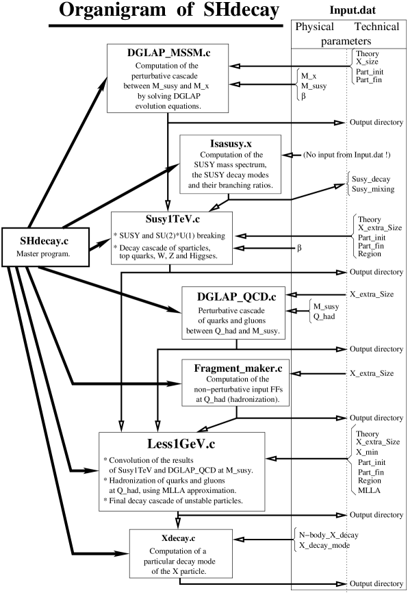
Figure 3.1: Organigram of SHdecay with the interdependence between the different programs and the needed input parameters for each code.

3.2.1 Technical parameters

• “$X_{\rm Size}$” gives the number of $x$ values used to store the FFs on the interval [$10^{-7}$:$1-10^{-7}$]. Because of a) the behavior of the splitting functions at small $x$, b) the fact that we are beginning with “delta functions” at large $x$, and c) the definition of the convolution which is relating the low and large $x$ regions, the two extremities of our interval have to be modeled symmetrically with great accuracy, if we want the integration and (cubic spline) extrapolation procedures to be able to give results at the desired precision of $\sim 10^{-3}$. For this purpose we used a bi-logarithmic scale between [$10^{-7}$:0.5] and [0.5:$1-10^{-7}$], increasing the number of $x$ values towards the two extremities. We are using by default $X_{\rm Size}=101$, i.e. 50 $x$ values on each side of the central value at $x=0.5$. Note that a smaller value could lead to false results, while increasing $X_{\rm Size}$ is increasing greatly the running time needed by all programs. So I really advise the user not to change this value. Note finally that the smallest $x$ value $10^{-7}$ has been chosen at the limit of the validity of the (leading order) DGLAP equations, before MLLA effects become strong (which happens at $\sqrt{\frac{Q_{had}}{M_{X}}}\sim 10^{-8}$ for $M_{X}\sim 10^{25}$ eV and $Q_{had}\sim 1$ GeV; see [19]). At low $x$, the standard LO DGLAP equations will predict a power law behavior (option MLLA = 0), but the MLLA approximation (option MLLA = 1) allows to parameterize some NLO effects like soft gluon emission.

• “$X_{\rm extraSize}$” is a parameter which allows the user to increase homogeneously the overall number of $x$ values on the interval $[10^{-7}:1-10^{-7}]$ after the first program DGLAP_MSSM (which is, once again, the most time consuming part of the complete code) has been completed. But it is quite useless, the initial value of $X_{\rm Size}$ being large enough for all following programs. By default, $X_{\rm extraSize}$ is simply taken to be equal to $X_{\rm Size}$. (Of course, it has to be greater than (or at least equal to!) $X_{\rm Size}$).

• “Part_init” and “Part_fin” describe the initial and final id’s of an interval of initial particles for which the FFs have to be computed. Note that there are 30 initial “compound” particles in the MSSM, and all the $30\times 30=900$ FFs from any particle to any other will be needed for the computation of the whole cascade. Thus the default values are respectively Part_init $=1$ and Part_fin $=30$, which means that the program will treat successively all the 30 possible initial particles. Nevertheless, the treatment of an initial particle being fully independent of the others, any of the 3 programs DGLAP_MSSM, Susy1TeV and Less1GeV can be cut into pieces to be run independently on different computers; for example, you can let a first computer run the chosen program for particles 1 to 15, and another computer run the same program for particles 16 to 30. These two parameters render this task easy and allow to save a lot of time.
  Caution: Note that each of these three programs has to be run over the whole range of particles before running the following one!

• $X_{\rm min}$ gives the lowest value of the final x interval. As stated above, in the lowest x region ($[X_{\rm min}:10^{-7}]$), you can choose two different extrapolations of the FFs: either extrapolating the power law obtained from the LO DGLAP equations, or using the MLLA approximation for taking color coherence effects into account. This parameter, taken by default to be $X_{min}=10^{-13}$, is only used in the very last part of the computation of the cascade: Less1GeV.
  Caution: of course, $X_{\rm min}$ has to be $\geq 10^{-7}$.

3.2.2 DGLAP_MSSM

This program treats completely the perturbative cascade above the $M_{\rm SUSY}$ scale. Starting from input FFs at $M_{\rm SUSY}$ for each type of primary particle $P$ ($D_{P}^{P}(x,M_{\rm SUSY})=\delta(1-x)$ and $\forall j\neq P$, $D_{P}^{j}(x,M_{\rm SUSY})=0)$, it gives the FFs of the 30 interaction eigenstates at scale $Q=M_{X}$: $D_{P}^{j}(x,M_{X})$.

By giving the parameters of the “Input.dat” file, the user can choose one of the 4 available theories, namely 1: MSSM, 2: SM, 3: SUSY-QCD, 4: QCD alone. I point out that this complicated program is certainly not the best one for treating a case as simple as QCD DGLAP equations (or even SUSY-QCD), being unfortunately quite time consuming. This program requires no external input (except Input.dat, of course), and only needs as “physical inputs” the values of $\beta$ and $M_{X}$, described above. The technical parameters $X_{\rm Size}$, “Part_init” and “Part_fin” are used, too. As I already mentioned before, I strongly suggest when possible to run the program on different computers at the same time, using different intervals of initial particles, for saving time.

Finally, the user should specify the corresponding output directory, where the output files will be stored.

Using the structure of the DGLAP evolution equations and $\delta$-functions as input FFs at $M_{\rm SUSY}$ (practically implemented as sharp Gaussians), this program will compute the full set of FFs from one particle to another between $M_{\rm SUSY}$ and $M_{X}$. For this purpose, we use a Runge-Kutta method with a constant logarithmic step in virtuality for solving the system of DGLAP equations. There must be an entire number of these steps between $M_{SUSY}$ and (any value of) $M_{X}$. That’s why it is only possible to use powers of 10 for these scales. Nevertheless, as I said before, this allows already a good accuracy.

Here we can see the interest of the variable “Nb_output_virtualities” and the corresponding array of virtuality values “Output_virtualities_DGLAP_MSSM”: thanks to the fact that this program is computing the FFs from $M_{SUSY}$ to $M_{X}$ through a given number of Runge-Kutta steps, all intermediate virtualities used by the Runge-Kutta program are available as possible outputs; it allows to get the FFs at intermediate virtualities, which are equivalent to lower $X$ masses $M_{X}$. As stated above, the step used for Runge-Kutta is a constant logarithmic step, exactly one order of magnitude each. So practically, the user who wants to study a GUT $X$ particle with mass $M_{X}\sim 10^{25}$ eV can get the results for any other (power of 10) $X$ mass ($10^{21}$, $10^{22}$, $10^{23}$ eV,…) between $M_{SUSY}$ and $M_{X}$. The two variables cited above allow to put these partial results in output files that will be usable later on. Note again that only this program will use the array of values for $M_{X}$. The following ones will simply use one of these values, the one given in the parameter $M_{X}$ itself.

The output is presented in $30\times 30=900$ files giving the FFs of any particle into any other with $X_{\rm Size}$ values of $x$ in the first column and the corresponding values of the FF in the second one. These files are called generically “fragment_(M_X)eV_p1.p2” for the FF of particle p1 into particle p2, where (M_X) contains the mass of the $X$ particle at which the FF was computed. Note that, according to the form of DGLAP equations for a generic FF $D_{p1}^{p2}(x,Q)$, the iterator part $\in[$Part_init,Part_fin$]$ of the program DGLAP_MSSM (and evidently its “brother” DGLAP_QCD) runs over the “final” particles p2. On the contrary, the equivalent iterators in Susy1TeV and Less1GeV run over particles p1. That’s why it is essential to run the different programs successively, after the complete end of the preceding one!.

Finally, it is worth noting that the output of this program only depends on very few parameters: the “theory” chosen as framework for the computation, the $M_{\rm SUSY}$ scale at which the perturbative cascade is ending, and the SUSY parameter $\tan\beta$. Yet, we have seen in section 2.3.3 that these two parameters have very little influence on the final results

. Thus I strongly recommend to let run this program only once, for all $X$ masses you want to study, and to carefully keep these partial results for later use, for studying the influence of other parameters appearing in the following programs.

3.2.3 How to use Isasusy.x

The ISASUSY program, written in fortran 77, is a subset of the whole code called ISAJET . I refer to the user manual of ISASUSY [16] for information about how to use this program. But, as mentioned above, I fully implemented a personalized version of this code, which is available through the master program (option 7). For a given set of SUSY parameters specified by the user in SUSY.dat, it computes the complete SUSY spectrum (masses and mixing angles of all the sparticles, stored in the “Mixing.dat” file), and the allowed decay modes with the corresponding branching ratios (stored in “Decay.dat”). Both files will be stored in the Isasusy directory of SHdecay, and their names have to be given in the “SUSY.dat” input file.

Of course, you can get these files from any other available code providing the same information as ISASUSY, as long as you adapt the output format of this code in order to get the one required by SHdecay (see the model files provided in the Isasusy directory for information about the required format). The furnished version of Isasusy is the one included in Isajet 7.51. If you want to use an updated version of Isasusy, you probably just need to replace the two files called “aldata.f” and “libisajet.a” in the Isasusy repertory of SHdecay (but hopefully not ssrun.f and the Makefile, which I have adapted).Yet, I obviously cannot ensure that this operation will work…

3.2.4 Susy1TeV

This program takes the results of DGLAP_MSSM given at the (unique) $M_{X}$ value specified in Input.dat and deals with the breaking of SUSY and $SU(2)\otimes U(1)$, the supersymmetric decay cascade and the decays of the top quarks, the Higgs, $W$ and $Z$ bosons. The muons and taus existing at this step are decayed too. We considered only 2- and 3-body decays for which we computed the relevant phase space (see Appendix C for details), using the branching ratios and the mass spectrum given by ISASUSY. For any detail on these procedures, we refer to [19].

The input directory has to be the one where the outputs of DGLAP_MSSM have been stored (the user doesn’t have to specify it). On the other hand, the output directory can be different, in order to distinguish between different parameters. For example, the mass of the $X$ particle, which is especially specified in the names of the output files of DGLAP_MSSM (as being the final virtuality of the perturbative cascade) is no more specified in the outputs of Susy1TeV; thus it can be useful to define different output directories for different $X$ masses. Moreover, the large number of output files is easier to handle when stored in different directories.

The program will need the two output files given by Isasusy.x (or any other program, see above); the two files have to be located in the directory “Isasusy”, and their names have to be given in the two corresponding parameters of SUSY.dat: “Decay” and “Mixing”. Here the parameter “Region” also becomes useful. If necessary, the extension of the $x$ array to “$X_{\rm extraSize}$” values instead of “$X_{\rm Size}$” will occur in this program, too.

The output files contain the FFs of the 30 initial particles (interaction eigenstates) into the remaining SM mass eigenstates after the decays, namely the quarks u, d, s, c, b and gluons, the electrons, neutrinos and the LSP. All of them will have a suffix “_1TeV” to distinguish them from the outputs of other programs and the “Region”-suffix, e.g. labeling the set of SUSY parameters you used during the run, or the $X$ mass you used (or both!).

3.2.5 DGLAP_QCD

This program is a simplified copy of DGLAP_MSSM. It computes the pure QCD perturbative partonic cascade for quarks and gluons (so only 6 particles) for a virtuality decreasing from $M_{\rm SUSY}$ to $Q_{\rm had}={\rm max}(m_{\rm quark},1$ GeV). This program is not using any previous result from other ones, and only depends on $M_{\rm SUSY}$ and $Q_{\rm had}$, which are not very sensitive parameters, as stated above. We thus recommend to define their values once and for all (say, keep the default values $M_{\rm SUSY}=1$ TeV and $Q_{\rm had}=1$ GeV), and to run DGLAP_QCD only once. This possibility of sparing running time is the reason why the necessary convolution between the results of this program and the FFs given by the previous one (Susy1TeV) was implemented in Less1GeV, in order to keep DGLAP_QCD fully independent.

The $6\times 6=36$ output files, called generically “fragment_p1.p2” - where p1 and p2 are initial and final partons {u,d,s,c,b,g} - will be stored in the corresponding directory given in Input.dat. We recommend to use a dedicated directory, for the reason stated above: these results are almost parameter independent and can be used for different runs of Susy1TeV and Less1GeV.

3.2.6 Fragment_maker

This program is certainly the weakest part of our treatment, because of the lack of knowledge concerning the non-perturbative FFs at very low $x$. We used the results of [17] for this purpose, which are based on LEP data. Unfortunately they are only valid for $x\geq 0.1$. The reason is that at LEP energies, it is necessary to consider mass effects at small $x$, which can be described by the so-called “MLLA plateau” (see section 2.3.4). Such effects can be taken into account during the computation of the hadronization itself, in Less1GeV. In Fragment_maker, we just keep the FFs given in [17] up to $x=0.1$ and extrapolate them at small $x$, by requiring continuity and the overall conservation of energy.

We finally obtain a set of input functions for light quarks (including the $b$) and for gluons which conserve energy and agree with known data.

This program is fully independent of the others, and is just used to “prepare” the non-perturbative input FFs at low energy needed in Less1GeV. It doesn’t depend on any parameter, and can be run once and for all. Once again, we recommend to use a dedicated directory for storing the output Files of this program; the default value is a directory called “Fragment”.

3.2.7 Less1GeV

This program first computes the convolution between the results of Susy1TeV (describing the evolution of the FFs between $M_{X}$ and $M_{\rm SUSY}$ after SUSY, top, $W$, $Z$ and Higgs decays) and the ones of DGLAP_QCD (describing the further evolution of the partonic part of these FFs between $M_{\rm SUSY}$ and $Q_{\rm had}$). It further deals with the hadronization of quarks and gluons, using external input FFs (The results of the Fragment_maker program described above) which have to be convoluted with the previous results. It finally deals with the decays of the last unstable particles. The 2- and 3-body decays are treated exactly as in Susy1TeV.

The results are once more given in terms of FFs of any initial (interaction eigenstate) particle (between the 30 available in the MSSM, see Appendix E) into the final (physical) stable ones, namely the protons, electrons, photons, three species of neutrinos, and LSPs. To simplify the storing and further use of these (final) results, we grouped all the results corresponding to one initial particle in one file generically called “fragment_p1.all_Region”, where p1 is the initial particle and Region the suffix labeling the set of SUSY parameters. Each file contains seven FFs: the first column gives the values of $x$ (from $1-10^{-7}$ to $X_{\rm min}$, in decreasing order), and the next columns give successively the FFs of p1 into protons, photons, LSPs, electrons, $\nu_{e}$, $\nu_{\mu}$, $\nu_{\tau}$.

3.2.8 Xdecay

This last program allows to study a special decay mode of the X particle, by computing a last convolution between the results obtained in Less1GeV and the phase space of the given decay mode. The number of decay products and their nature (through the associated id, see Appendix E) have to be specified in Input.dat.

If a decay mode for the $X$ particle has been specified in the two parameters “N-body_X_decay” and “X_decay_mode” (respectively the number $N$ of products and the id’s associated to each product - see Appendix E), a last convolution with the $N$-body decay energy spectrum will be computed and the results will be directly given in terms of the FFs of the $X$ particle into the stable final ones. The $N$-body energy spectrum we used is the one given in [26]. If $\rho_{N}(z)$ is the probability density of obtaining a decay product of energy $E$ carrying the energy fraction $x=2E/M_{X}$ of the decaying particle, we have:

$$\rho_{2}(x)=\delta(1-x)\,,$$

$$\rho_{N}(x)=(N-1)(N-2)x(1-x)^{N-3}\,,N\geqslant 3\,.$$

This program has been separated from Less1GeV to allow the user to obtain very quickly any decay mode he wants to study. The final result is stored in the same directory as the results of Less1GeV. It is generically called “frag_X_a_b_c.all_Region” (see section 3.1.4) and has the same format as the one described above for the results of Less1GeV.

3.3 Conclusion

This chapter describes in some detail how to use the code SHdecay, which has been designed for computing the most general decay spectra of any super-heavy particle in the framework of the MSSM. I hope that it will be of some use for other researchers. As I mentioned before, the code as well as a version of this user-guide are available on the web site of our group, under the address: ”www1.physik.tu-muenchen.de/$\sim$barbot/”, and I will be pleased to answer any question you have about it. Of course, any remark or suggestion is welcome, too.

Chapter 4 Applications of SHdecay: phenomenology

4.1 Introduction

Since the first discovery of cosmic rays (CRs) in 1912 by Victor Hess[45], their energy spectrum has been measured over more than 12 decades of magnitude. Although there still are number of discussions going on in this field of research, our general understanding of the typical features of this spectrum has greatly improved. Especially, these CR particles are now known to consist primarily of protons, helium, carbon, nitrogen and other heavy ions up to iron.

Above $10^{14}$ eV, the flux becomes so low that only ground-based experiments with large aperture and long exposure times can hope to acquire a significant number of events. Such experiments exploit the atmosphere as a giant calorimeter. The incident cosmic radiation interacts with the atomic nuclei of air molecules and produces extensive air showers (EAS) which spread out over large areas. Already in 1938, Pierre Auger concluded from the size of EAS that the spectrum extends up to and perhaps beyond $10^{15}$ eV [46, 47]. Nowadays substantial progress has been made in measuring the extraordinarily low flux ($\sim 1$ event km^-2 yr^-1) above $10^{19}$ eV. Continuously running experiments using both arrays of particle detectors on the ground like AGASA and fluorescence detectors which track the cascade through the atmosphere like HiRes, have detected events with primary particle energies higher than $10^{20}$ eV [6, 7, 8, 9, 10, 11, 12, 13], with no evidence that the highest energy recorded thus far is Nature’s upper limit (see fig. 4.1).

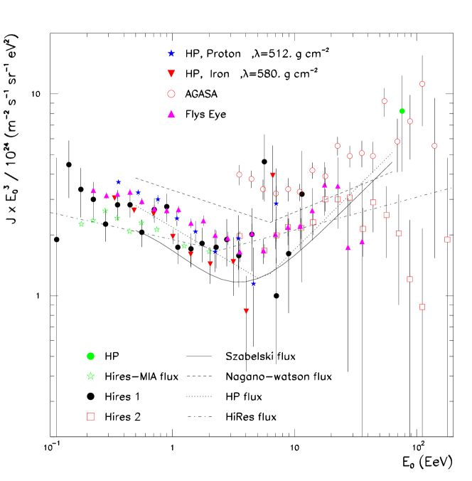
Figure 4.1: A composite energy spectrum including recently reanalyzed Haverah Park data assuming proton and iron primaries (the parameter $\lambda$ measures the attenuation length of the density of charged particles at 600 m from the shower core), stereo Fly’s Eye data, monocular HiRes data from both eyes up to $60^{\circ}$, and hybrid HiRes–MIA data. Published in Ref. [48].

Such tremendous energies, well above the energies that we can expect to reach on Earth in the current and future generations of colliders, defy our understanding for number of reasons; in particular, CRs of energies beyond the ankle ($\sim 10^{18}$ eV) are expected to be of extragalactic origin, and probably coming from distances further than the local cluster of galaxies ($\sim 20$ Mpc), because we know no astrophysical object able to accelerate particles enough to provide them such an energy in our vicinity. Yet, particles carrying energies above $10^{20}$ eV traveling over cosmological distances should lose their energy through propagation effects; for example, a proton will interact with the cosmological microwave background (CMB) and photoproduce pions, with an interaction length of a few tens of Mpc, losing around 20 % of its energy at each interaction. Similar processes occur with nuclei, photons (through gamma-gamma pair production over the radio background (URB) essentially) or electrons (Inverse Compton scattering over the URB). Thus particles with initial energy $\sim 10^{20}$ eV coming from cosmological distances (over 50 Mpc) should reach the Earth with a maximal energy $\sim 5.10^{19}$ eV, as it was already predicted independently by Greisen [49], and Zatsepin and Kuzmin [50] in 1966; the expected fall off of the spectrum is nowadays referred as the GZK cut-off. Yet, events have been registered above this cut-off in very different experiments over the last few decades [6, 9, 8, 51, 10, 11, 12, 54]. A recent review of the experimental results is also given in [55].

The presence or absence of this cut-off in the CR spectrum is still a matter of controversy: as one can see from fig. 4.1, if it seems to be present in the updated HiRes spectrum [13], it is fully absent in the AGASA one [10]. But all experiments agree on the existence of events well above this cut-off; this result is certainly the strongest argument against the classical” acceleration (or “bottom-up”) theories, which are usually recognized to be the most efficient mechanism for producing the CR spectrum at lower energies. Indeed, the bottom–up theories exploit the electromagnetic fields that are likely to be present in objects like gamma ray bursters [56], “hot spots” of radio-galaxies [57] or near super–massive black holes in dormant quasars [58] in order to accelerate charged particles. However, it is difficult to find objects capable of accelerating protons to energies above $10^{20}$ eV, partly because the product of field strength and spatial extension of the field does not seem to be sufficiently large, and partly because the accelerated particles can loose a fair fraction of their energy in synchrotron radiation. Moreover, there is another strong indication against these models: UHECRs are expected to travel rather straight away in the universe, without being deviated by the (inter)galactic magnetic fields. Thus they should point to there sources within a few degrees. Yet, excepted the existence of a few doublets and triplets in the experimental data, the observations are compatible with an almost perfect isotropy above $4.10^{19}$ eV [52].

These remarks lead to the development of another class of models attempting to explain the existence of UHECRs, generically called “top-down” theories. Here one postulates the existence of “new physics” at a very high energy scale, i.e. the existence of super-heavy particles of masses greater than $10^{12}$ GeV, which could decay and hence produce the observed UHECRs. Top–down models can be motivated by a variety of arguments. For example, the recent measurements of the cosmic microwave background and of supernova redshifts have dramatically confirmed that our universe contains a large fraction of cold dark matter [59]. A top–down model in which annihilating or decaying superheavy relic particles produce the highest energy cosmic rays could potentially solve both of these problems [60, 22, 61]. Several mechanisms for the production of such ultra–massive particles at the end of inflation have been suggested [5]. Moreover, particles with the required mass and lifetime are predicted to exist in certain superstring theories [62]. Another explanation for the required long lifetime of these particles is to confine them into topological defects [21]. These ideas have been lengthy reviewed e.g. in [3, 4, 63, 64].

In this chapter, we will focus on this last class of models, in order to see which quantitative predictions we can make within our current knowledge, using the results presented in the previous chapters. We will see that is it possible to make testable predictions for both neutrino and LSP fluxes which could be observed on Earth in the next generation of experiments, thus providing a way to reinforce or rule out this class of models.

4.2 What can we learn?

As we have seen in chapter 3, the SHdecay code provides the spectra of the stable particles at source, from the decay of a unique X particle. In order to make predictions on the real fluxes that could be observed on Earth in the current and future detectors, we need a complete model for the UHECR production and propagation, which includes:

• A given model of $X$ particles, specifying the nature of the $X$ particle, or at least its decay modes (with their branching ratios) - and possibly its lifetime.

• A cosmological model for $X$ particles production and evolution which allows to determine their current distribution in the universe.

• A propagation code for all types of stable particles produced in the decay, taking into account the travel distances, the galactic and intergalactic magnetic fields, and all leading interactions between the UHECRs and the different backgrounds (CMB, infrared, radio).

• An “extensive air shower” code for each kind of initial particles.

• A good knowledge of the detectors, especially their acceptances, exposure times and efficiencies, and a good study of all possible backgrounds for a given signal.

Of course, in our current understanding of these problems, the estimations that can be done are extremely model dependent. Yet, we can parameterize our ignorance and use the current known data to partly get rid of this model dependency. In particular, we certainly don’t need to know all details related to the $X$ particle for pursuing the study: we can consider a few typical decay modes (hadronic/leptonic/bosonic with small or large number $N$ of decay products), and different typical distributions of $X$ particles in the universe, independently of the whole story of their production and evolution since the very early ages of the universe. In order to get the required density of sources, we simply can normalize our spectra on the available data for a given type of observed particles, and use this parameterization for making predictions on the fluxes of other particles. In the next sections, we will follow this phenomenological procedure in order to get “order of magnitude” predictions for the neutrino and neutralino fluxes on Earth.

There is one more point that we have to address here before going further: in order to make quantitative predictions on the neutrino and neutralino fluxes that could be observed on Earth, we need to make an assumption on the composition of the observed UHECR spectrum.

Established particle physics implies that UHE jets fragment predominantly into pions and kaons, with a small admixture of protons [65]. The mesons will eventually decay into photons or electrons plus neutrinos. A typical QCD jet therefore produces more photons than protons. This is true in particular at relatively low values of $x=E_{\rm particle}/E_{\rm jet}$, but even at large $x$ the photon flux is at least as large as the proton flux in a jet [61, 66, 23, 22, 26]. This seems to be in disagreement with mounting evidence that the highest energy cosmic rays are not photons [42]. The observed shower profile of the original Fly’s Eye event [12], with energy exceeding $10^{20}$ eV, fits the assumption of a primary proton, or, possibly, that of a nucleus. The shower profile information is sufficient to conclude that the event is unlikely to be of photon origin [67]. The same conclusion is reached for the Yakutsk event that is characterized by a large number of secondary muons, inconsistent with a purely electromagnetic cascade initiated by a gamma ray. A reanalysis of Haverah Park data further reinforces this conclusion [68]. Very recently AGASA published [10] strong upper limits on the $\gamma/p$ ratio. Their data are compatible with being entirely due to protons, and strongly disfavor scenarios where most events are photonic in origin. This conclusion is again based on the observed number of muons in UHE showers, as well well as on the absence of a south–north asymmetry in the events. Such an asymmetry would be produced by $\gamma\rightarrow e^{+}e^{-}$ conversion in the Earth’s magnetic field, which becomes effective for $E_{\gamma}\geq 10^{19}$ eV. In light of this information, it seems likely that protons, and not gamma rays, dominate the highest energy cosmic ray spectrum. This strongly disfavors superheavy particles as the source of the highest energy cosmic rays, unless UHE photons are depleted from the cosmic ray spectrum near $10^{20}$ eV, leaving a dominant proton component at GZK energies. In fact, the uncertainties associated with the cascading of the jets in the universal and galactic radio backgrounds and with the strength of intergalactic magnetic fields leave this possibility open at least for sources at cosmological distances [3, 69]. If most relevant sources are located in the halo of our own galaxy, as expected for free nonrelativistic particles [22], one would have to assume that the galactic radio background has been underestimated by about an order of magnitude, which may not be impossible [70]. With this in mind, we will choose to normalize the proton spectrum from top–down scenarios to the observed UHECR flux. We recognize that this assumption may be somewhat extreme especially for local sources. However, we believe that it is necessary for the viability of this kind of model; and it is no more extreme than many other proposed explanations of the post–GZK events. Moreover, as we will see in the following sections, relaxing this assumption by allowing a possible fraction of UHE photons in the UHECR spectrum only reduces the predicted event rate by factors of two or three; this is less than the inherent uncertainty of our calculation, arising from the discrepancy in the current data and the unavoidable dependence on the unknown $X$ decay mode.

4.3 UHE neutrino fluxes on Earth: detection at the corner?

Neutrinos are produced more numerously than protons and travel much greater distances. Possible neutrino signals of top–down models have therefore been suggested quite a while ago [38]. Here we perform an up–to–date analysis of these signals in various kinds of detectors, using the most accurate available calculation of the neutrino fluxes at source (see chapter 2 or [18, 19]). Once we “renormalize” the observed cosmic ray flux to protons, we generically predict observable neutrino signals in operating experiments such as AMANDA II, RICE and AGASA. Top–down models, if not revealed, will be severely constrained by high–energy neutrino observations in the near future.

4.3.1 Nucleons from ultra-high energy jets

The assumption that nucleons from the decay (or annihilation) of very massive $X$ particles are the source of the highest energy cosmic rays normalizes the decay or annihilation rate of their sources, once the shape of the spectrum of the produced nucleons is known. One needs mass $M_{X}\geq 10^{21}$ eV in order to explain the observed UHECR events. The presence of such very massive particles strongly indicates the existence of superparticles with masses at or below the TeV scale, since otherwise it would be difficult to keep the weak energy scale ten or more orders of magnitude below $M_{X}$ in the presence of quantum corrections. Moreover, we know that all gauge interactions are of comparable strength at energies near $M_{X}$. These two facts together imply that the evolution of a jet with energy $\geq 10^{21}$ eV shows some new features not present in jets produced at current particle collider experiments.

First of all, primary $X$ decays are likely to produce approximately equal numbers of particles and superparticles, since $M_{X}$ is much larger than the scale $M_{\rm SUSY}\leq 1$ TeV of typical superparticle masses. Even if the primary $X$ decay only produces ordinary particles, superparticles will be produced in the subsequent shower evolution [23, 26]. Note also that (at least at high energies) electroweak interactions should be included when modeling the parton shower. Both effects taken together imply that the jet will include many massive particles – superparticles, electroweak gauge and Higgs bosons, and also top quarks. The decays of these massive particles increase the overall particle multiplicity of the jet, and also produce quite energetic neutrinos, charged leptons and lightest supersymmetric particles (LSPs). Eventually the quarks and gluons in the jet will hadronize into baryons and mesons, many of which will in turn decay.

We model these jets at the point of their origin using SHdecay. The results presented below have been obtained using a “typical” spectrum with superparticles in the hundreds of GeV region; the dependence of the predicted neutrino fluxes on the spectrum of superparticles is much weaker than that on the primary $X$ decay mode discussed below. At virtualities below $M_{\rm SUSY}$ only ordinary QCD interactions contribute significantly to the development of the jet; $b$ and $c$ quarks are decoupled at their respective masses, hadronize, and decay. At a virtuality near $1$ GeV the light quarks and gluons hadronize, with a meson to baryon ratio of roughly thirty to one (five to one) at small (large) $x$. All baryons will eventually decay into protons, while the mesons (mostly pions) decay into photons, electrons and neutrinos (plus their antiparticles). The heavier charged leptons (muons and taus) also decay. The final output of the code is the spectra of seven types of particles which are sufficiently long–lived to reach the Earth: protons, electrons, photons, three flavors of neutrinos, and LSPs. We assume that $X$ decays are CP–symmetric, i.e. we assume equal fluxes of particles and antiparticles of a given species.

The first version of SHdecay (as presented in Ref.[18]) was based on conventional one–loop evolution equations for the relevant fragmentation functions. These may not be reliable in the region of very small $x$. We wish to calculate neutrino fluxes at energies down to $\sim 10^{15}$ eV (1 PeV), which corresponds to $x\sim 10^{-6}\ (10^{-10})$ for $M_{X}=10^{21}\ (10^{25})$ eV. At these very small $x$ values color coherence effects are expected to suppress the shower evolution [71]. We tried to estimate the size of these effects by matching our spectra computed using conventional evolution equations to the so–called asymptotic MLLA spectra (see section 2.3.4 of chapter 2). The effect of this modification on the neutrino event rate is relatively modest for primary jet energy near $10^{21}$ eV, but becomes significant at $10^{25}$ eV. However, even at this higher energy the proton flux, which we only need at $x\geq 10^{-5}$, is not affected significantly.

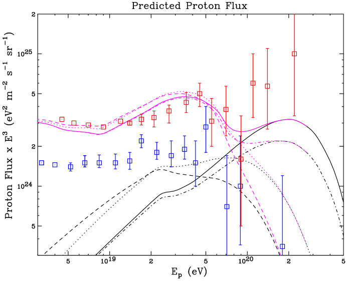
Figure 4.2: The ultra high–energy cosmic ray flux predicted for the decay of superheavy particles with mass $M_{X}=2\cdot 10^{21}$ eV is compared to the HiRes (darker) and AGASA (lighter) cosmic ray data. The distribution of jets used includes an overdensity factor of $10^{5}$ within 20 kpc of the galaxy. Spectra are shown for quark$+$antiquark (solid), quark$+$squark (dot–dash), $SU(2)$ doublet lepton$+$slepton (dots) and 5 quark$+$5 squark (dashes) initial states. Dark (lower) lines are from top–down origin alone whereas lighter (upper) lines are top–down plus an homogeneous extragalactic contribution as predicted in Ref.[3]. Note that all observed super GZK events can be explained by this mechanism.

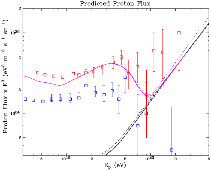
Figure 4.3: As in figure 4.2, but using particles of mass $M_{X}=2\cdot 10^{25}$ eV.

This calculation gives us the shape of the spectra of the stable particles at source. The spectra on Earth might differ significantly due to propagation effects. As stated in section 4.2, we will assume that (almost) all UHE photons get absorbed. This is actually expected to be true for a homogeneous source distribution. However, according to current estimates of the strengths of the magnetic fields and of the radio wave background in (the halo of) our own galaxy most UHE photons produced in the halo of our galaxy are expected to reach the Earth. As we already saw, this seems to be in conflict with observation. We will therefore assume that the interaction length of UHE photons in our galaxy has been greatly over–estimated, and explore the consequences of this assumption for neutrino signals.

As well known, (anti)protons lose energy when traveling through the intergalactic medium, mostly through scattering off photons of the ubiquitous cosmic microwave background (CMB). We calculate the observed spectrum of protons taking into account scattering off the CMB at the $\Delta-$resonance and scattering by $e^{+}e^{-}$ pair production; energy losses through the Hubble expansion of the Universe are also included [3, 72]. Note that the photoproduction of charged pions contributes to the observed neutrino flux on Earth. In order to solve the ultra high–energy cosmic ray problem, the (anti)proton flux must accommodate the events above the GZK cutoff. Observations indicate on the order of a few times $10^{-27}$ events $\rm{m}^{-2}\rm{s}^{-1}\rm{sr}^{-1}\rm{GeV}^{-1}$ in the energy range above the GZK cutoff ($5\times 10^{19}$ eV to $2\times 10^{20}$ eV).

The formalism of a generic top–down scenario is sufficiently flexible to explain the data from either the HiRes [13] or AGASA [10] experiments. Figure 4.2 compares HiRes and AGASA data to the proton spectrum predicted for a galactic distribution of decaying particles with mass $M_{X}=2\cdot 10^{21}\,$ eV. The drop near a few times $10^{19}$ eV is a manifestation of the GZK cutoff. Note, however, that there are sufficient semi–local events to explain all observed super GZK events. Similarly, figure 4.3 compares HiRes and AGASA data to the spectrum predicted for $M_{X}=2\cdot 10^{25}$ eV, rather than $2\cdot 10^{21}$ eV, decaying particles for the same distribution. Although HiRes and AGASA data differ at face value, especially above the GZK cutoff, top–down scenarios can accommodate all events observed above the GZK cutoff in either experiment.

If the cosmic ray sources are not distributed with a large overdensity in the galaxy, the resulting cosmic ray and neutrino spectrum will be modified. For example, using a homogeneous distribution, the GZK cutoff will again be manifest and the observed cosmic ray spectrum will be difficult to explain. A galactic overdensity of $10^{3}$ to $10^{4}$ or more seems necessary to fit the data. The figure 4.2 shows a $10^{5}$ overdensity, which is the overall overdensity of matter in our galaxy at the location of the Sun. Note that for less extreme over-densities, the average distance at which a proton is produced will be larger. This implies larger energy losses, and hence a reduced proton flux on Earth for a given number of sources. Conversely, if we fix the proton flux to the observed flux of UHECR events, models with lower overdensity require more sources. Since neutrino fluxes are not degraded by propagation through the intergalactic medium, the number of neutrinos increases proportionally to the number of sources, with additional contributions to the neutrino flux coming from pion production on the CMB background. Thus, the neutrino event rates and spectrum shown in the figures reflect the most conservative choice of distributions. Table 4.1 shows results for both homogeneous and galactic distributions.

4.3.2 Neutrinos from ultra-high energy jets

Neutrinos, not being limited by scattering, travel up to the age of the universe at the speed of light ($\sim$ 3000 Mpc in an Euclidean approximation). The only nontrivial effect of neutrino propagation is due to oscillations. In our case the propagation distance of neutrinos amounts to many oscillation lengths, if oscillation parameters are fixed by the currently most plausible solutions of the atmospheric and solar neutrino deficits [73]. As a result, the UHE neutrino flux on Earth is the same for all three flavors, and amounts to the average of the fluxes of the three neutrinos flavors at source.

The predicted neutrino flux is shown in figures 4.4 and 4.5. At $E_{\nu}\ll E_{\rm jet}$ the main contribution comes from $\pi^{\pm}\rightarrow\mu^{\pm}\nu_{\mu}\rightarrow e^{\pm}\nu_{e}\nu_{\mu}$ decays, but at larger $E_{\nu}$ there can be significant contributions from the decays of heavy (s)particles. The peak in the dotted curves at $E_{\nu}=E_{\rm jet}$ results from our assumption that in this scenario $X$ decays directly into first or second generation $SU(2)$ doublet (s)leptons, which implies that 50% of all $X$ decays give rise to a primary neutrino; in this case the ratio of neutrino and proton fluxes has a maximum at high energy. On the other hand, if primary $X$ decays are purely hadronic, the neutrino flux at the largest energy is only slightly above the proton flux at that energy. The reason is that neutrinos from meson decays only carry a fraction of the energy of the meson, so a five to one meson to proton ratio at large $x$ leads to a nearly one to one neutrino to proton ratio. We see that the neutrino flux at the highest energy depends quite strongly on how the $X$ particles decay; there is also some dependence on the parameters of the SUSY model [18, 19]. For given proton flux the neutrino flux at smaller $x$ is much less model dependent. At very small $x$ a new uncertainty appears due to coherence effects. These have so far only been studied in a pure QCD parton shower; our treatment of these effects is therefore of necessity rather crude.

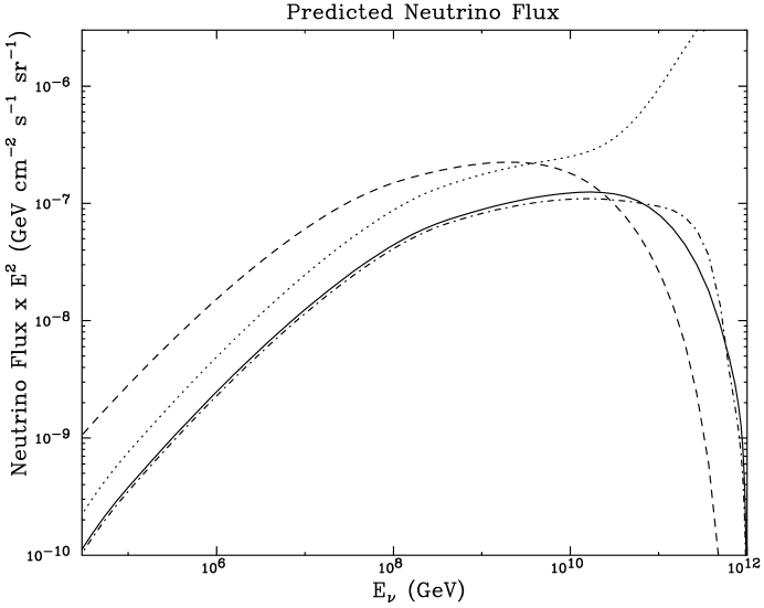
Figure 4.4: The neutrino plus anti–neutrino flux corresponding to the cosmic ray spectra of figure 4.2 from the decay of superheavy particles with mass $M_{X}=2\cdot 10^{21}$ eV. Spectra are shown for quark–antiquark (solid), quark–squark (dot–dash), lepton–slepton (dots) and 5 quark–5 squark (dashes) initial states.

Figure 4.5: As figure 4.4, but corresponding to the cosmic ray spectrum of figure 4.3 with $M_{X}=2\cdot 10^{25}$ eV.

4.3.3 Event rates in high-energy neutrino telescopes and air shower experiments

We will discuss two classes of experiments capable of observing high energy cosmic neutrinos: neutrino telescopes and air shower experiments.

Optical Cerenkov neutrino telescopes such as the operating AMANDA II and next generation IceCube [74] are designed to observe muon tracks from charged current interactions as well as showers which occur in the detector. The probability of detecting a neutrino passing through the detector from its muon track is given by

$$P_{\nu\rightarrow\mu}(E_{\nu},\theta_{\rm zenith})=\sigma_{\nu N}(E_{\nu})\,n_{\rm{H_{2}O}}\,R_{\mu}(E_{\mu},\theta_{\rm zenith}),$$ (4.1)

where $n_{\rm{H_{2}O}}$ is the number density of nucleons in the detector medium (water or ice), and the muon range $R_{\mu}(E_{\mu},\theta_{\rm{zenith}})$ is the average distance traveled by a muon of energy $E_{\mu}$ before falling below some threshold energy (we have used 100 TeV). This quantity depends on the zenith angle of the incoming neutrino because for a detector depth of $\sim 2\,$km, only quasi–horizontal or upgoing events can benefit from longer muon ranges. At the energies we are most concerned with, the majority of muon events will be quasi–horizontal. The number of muon events observed is then given by

$$N_{\rm{events}}=\int dE_{\nu}\,d\Omega\,\frac{d\phi_{\nu}}{dE_{\nu}}\,P_{\nu\rightarrow\mu}(E_{\nu},\theta_{\rm zenith})\,A_{\rm eff}\,T,$$ (4.2)

where $T$ is the time observed and $A_{\rm{eff}}$ is the effective area of the detector: one twentieth square kilometers for AMANDA II and one square kilometer for IceCube.

AMANDA II and IceCube can also observe showers generated in charged or neutral current interactions within the detector volume. The event rate from showers is not enhanced by long muon ranges, but can be generated by all three flavors of neutrinos and with greater cross section (neutral + charged current). We use a shower energy threshold of 100 TeV. The energy threshold imposed effectively removes any background events from atmospheric neutrino events. For a review of Optical Cerenkov neutrino telescopes see Ref.[75].

The operating radio Cerenkov experiment, RICE, is capable of observing showers generated in charged current electron neutrino events. RICE’s effective volume increases with energy. At 1 PeV, RICE has an effective volume less than one hundredth of a cubic kilometer. At higher energies, however, it increases to about ten cubic kilometers [76].

Air shower experiments can also observe very high energy cosmic neutrinos. We consider AGASA, the largest ground array currently in operation [53], and the next generation AUGER array [77].

To determine that an air shower was initiated by a neutrino, rather than a proton or other cosmic ray, we require a slant depth greater than 4000 $\rm{g}/\rm{cm}^{2}$. This corresponds to a zenith angle near 75 degrees. Therefore, only quasi–horizontal air shower events can be identified as neutrinos. Additionally, unlike showers generated in the upper atmosphere, deeply penetrating showers provide both muon and electromagnetic shower components which help them be differentiated from showers with hadronic primaries. The probability of detecting and identifying a neutrino initiated air shower is described in terms of the array’s acceptance, $A$, in units of volume times water equivalent steradians (we sr). The detector’s acceptance increases with energy. For AGASA, the acceptance is about $0.01\,\rm{km}^{3}\,\rm{we}\,{sr}$ at $10^{7}\,$ GeV but increases to $1.0\,\rm{km}^{3}\,\rm{we}\,{sr}$ at $10^{10}\,$ GeV and above. For AUGER, the acceptance is about $0.1\,\rm{km}^{3}\,\rm{we}\,{sr}$ at $10^{8}\,$ GeV and reaches above $10.0\,\rm{km}^{3}\,\rm{we}\,{sr}$ by $10^{10}\,$ GeV. The number of events observed is then

$$N_{\rm events}=\int dE_{\nu}\,d\Omega\,n_{\rm{H_{2}O}}\,\frac{d\phi_{\nu}}{dE_{\nu}}\,\sigma_{\nu N}(E_{\nu})\,A(E_{\nu})\,T,$$ (4.3)

where $T$ is again the time observed, $n_{\rm{H_{2}O}}$ is the number density of nucleons in water and $A(E_{\nu})$ is the detector’s acceptance. AGASA presently has about five years of effective running time between 1995 and 2000 analyzed.

The AUGER array will also be capable of observing upgoing showers generated by tau neutrinos in the shallow earth. The rates for upgoing tau neutrinos events are typically about an order of magnitude higher than the rates for quasi horizontal downgoing neutrino events. For more a detailed description of air shower acceptances and rates from upgoing and quasi horizontal neutrino induced showers, see Ref. [78].

	Amanda II		Agasa		Rice		IceCube		Auger
$q\bar{q}$, $10^{21}$ eV, Gal	0.29		0.030		1.5		9.6		1.2
$q\tilde{q}$, $10^{21}$ eV, Gal	0.29		0.028		1.5		9.5		1.2
$5\times q\tilde{q}$, $10^{21}$ eV, Gal	0.97		0.065		3.5		32.1		2.9
$l\tilde{l}$, $10^{21}$ eV, Gal	0.50		0.079		3.9		16.1		2.5
$q\bar{q}$, $10^{25}$ eV, Gal	0.027		0.0094		0.38		0.80		0.29
$q\tilde{q}$, $10^{25}$ eV, Gal	0.026		0.0092		0.37		0.88		0.28
$5\times q\tilde{q}$, $10^{25}$ eV, Gal	0.034		0.010		0.42		1.0		0.33
$l\tilde{l}$, $10^{25}$ eV, Gal	0.029		0.011		0.42		0.87		0.32
$q\bar{q}$, no MLLA, $10^{25}$ eV, Gal	0.041		0.0099		0.40		1.2		0.31
$q\bar{q}$, $10^{21}$ eV, Hom	2.6		0.27		13.8		86.0		11.0
$q\tilde{q}$, $10^{21}$ eV, Hom	2.6		0.25		13.2		85.1		10.5
$~{}5\times q\tilde{q}$, $10^{21}$ eV, Hom	8.7		0.59		31.5		289.1		25.7
$l\tilde{l}$, $10^{21}$ eV, Hom	4.5		0.71		35.3		144.9		22.9
$q\bar{q}$, $10^{25}$ eV, Hom	0.40		0.14		5.7		12.0		4.3
$q\tilde{q}$, $10^{25}$ eV, Hom	0.39		0.14		5.6		11.7		4.2
$5\times q\tilde{q}$, $10^{25}$ eV, Hom	0.51		0.15		6.3		15.5		5.0
$l\tilde{l}$, $10^{25}$ eV, Hom	0.44		0.16		6.4		13.1		4.7
$q\bar{q}$, no MLLA, $10^{25}$ eV, Hom	0.62		0.15		5.9		18.5		4.6

Table 4.1: Neutrino events per year in top–down scenarios for several operating and next generation experiments. For AMANDA II and IceCube, 100 TeV shower and muon energy thresholds were imposed. Events are only calculated up to $10^{12}$ GeV as discussed in the text.

Table 4.1 shows the event rates expected for a variety of models, and for several experiments. AMANDA-II, with an effective area of $\sim$50,000 square meters can place the strongest limits on high energy neutrino flux presently. Furthermore, AGASA, with five years of effective observing time, has similar sensitivity. RICE, just beginning to release results, will be capable of raising the level to which top–down scenarios can be tested, perhaps being capable of testing many of the models shown in the table. Even if no events are observed with operating experiments, next generation experiments, such as IceCube and AUGER, will be able to test all models with adequate sensitivity.

Event rates shown in table 4.1 include only events below $10^{12}$ GeV. Above this energy, uncertainties in the neutrino–nucleon cross sections and in detector performance make such calculations difficult and unreliable. Our most reasonable extrapolations into this energy range indicate about a 20% enhancement to the event rate if all energies are considered for $10^{25}$ eV jets. There is no effect for the $10^{21}$ eV jet case.

High–energy neutrino event rates have been calculated in Ref. [79] for a similar model. Their calculation used the model of reference [60] which normalized the ultra high–energy cosmic ray flux to the photons and protons generated in superheavy particle decay rather than the proton flux alone. For this reason, their results show only two events per year in a square kilometer neutrino telescope, a smaller rate than we predict for most models. Another recent estimate of neutrino fluxes on Earth in top–down models [80] finds broadly similar results as our’s. However, there the ‘MLLA’ form for the fragmentation functions was used for all energies, which (incorrectly) predicts nearly energy–independent ratios of neutrino, photon and proton fluxes.

4.3.4 Conclusions

If a top–down scenario, such as the decay or the annihilation of superheavy relics, is the source of the highest energy cosmic rays, then a UHE neutrino flux should accompany the observed cosmic ray flux. This neutrino flux will be much higher than the flux of nucleons due to the much greater mean free path of neutrinos and greater multiplicity of neutrinos produced in high–energy hadronic jets.

The UHE neutrino flux generated in such a scenario can be calculated by normalizing the flux of appropriate particles to the UHECR flux. With mounting evidence that the highest energy cosmic rays are protons or nuclei and not photons, we have assumed that the UHE photons are degraded by the universal and/or galactic radio background, leaving protons to dominate the highest energy cosmic ray flux. The neutrino flux must then be normalized to the proton flux resulting in significantly improved prospects for its detection.

A word about the uncertainties in our calculation might be in order. First of all, the uncertainty of the measured UHECR flux, and in particular the discrepancy between the HiRes and AGASA results, leads to an overall uncertainty. On the theoretical side, the main uncertainty probably comes from the calculation of the particle spectra at “small” energies, where currently not very well understood coherence effects can play a role. This effect is bigger for higher primary jet energy, and can change the event rate by up to a factor of about 2 or less (see table 4.1). Relaxing our assumption that all UHE photons are absorbed would lead to a corresponding reduction of the fitted source density, and hence of the neutrino flux. In this context it is worth mentioning that in the scenario which seems to fit the data best, with primary jet energy near $10^{21}$ eV and a galactic source overdensity of about $10^{5}$ (see Fig. 4.2 and ref.[26]), including the photon flux fully would only reduce the predicted event rate by a factor of two to three, since in this case the flux of $10^{20}$ eV photons at source is only slightly larger than the corresponding proton flux. This would still give a neutrino flux in easy striking range of km² scale detectors.

This paper shows that the neutrino flux accompanying the highest energy cosmic rays in top–down scenarios is of order of the limits placed by operating experiments such as AMANDA II, RICE and AGASA. Further data from these experiments, or next generation experiments IceCube and AUGER, can test the viability of top–down scenarios which generate the highest energy cosmic rays. If a signal is found soon, future high statistics experiments should be able to map out the neutrino spectrum, thereby allowing us direct experimental access to physics at energy scales many orders of magnitude beyond the scope of any conceivable particle collider on Earth.

Note Added

After completion of this work HiRes published [13] updated spectra for both their own and the AGASA experiment. The new HiRes spectrum (which, however, does not include the original Fly’s Eye event [12]) is somewhat below the spectrum shown in Figs. 4.2 and 4.3; it shows clear evidence for a spectral break, as predicted by the GZK effect, and is thus consistent with a homogeneous distribution of sources. Ref.[13] also contains an updated AGASA spectrum, which at $E\sim 10^{20}$ eV is slightly higher than the one used in our fits. The discrepancy between these two experiments, and the resulting uncertainty of the UHECR proton flux, is thus larger than previously anticipated. Note, however, that going from a galactic to a homogeneous distribution of sources can over–compensate the reduced normalization of the proton flux indicated by the HiRes spectrum, as far as the rate for neutrinos with energy exceeding 100 TeV is concerned.

4.4 Detecting SUSY in the sky? A new window for neutralino detection

In models where the UHE cosmic ray problem is solved by top-down scenarios, a significant flux of UHE neutralinos is predicted. We calculate the number of events expected from such particles in future experiments such as EUSO or OWL. We show that by using the Earth as a filter, showers generated by neutralinos can be separated from neutrino generated showers. We find that for many models, observable rates are expected.

4.4.1 Ultra-high energy fragmentation to neutralinos

From the general results discussed in chapter 2, we found that the LSP flux depends only mildly on the spectrum of superparticles, as long as the LSP is a bino–like neutralino. Some sample spectra are shown in Fig. 4.6.

Here we have once again conservatively assumed that $X$ particles have an overdensity of $10^{5}$ in the vicinity of our galaxy, as expected [22] for $X$ particles that move freely under the influence of gravity. This minimizes the expected neutralino flux, since, as in the preceeding section, all scenarios are normalized by matching [39] the predicted proton spectrum to the highest energy cosmic ray observations (see discussion in section 4.2).

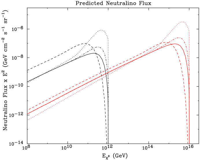
Figure 4.6: The spectrum of neutralino LSP’s predicted for the decay of superheavy particles with mass $M_{X}=2\cdot 10^{21}$ eV (left set of curves) and $M_{X}=2\cdot 10^{25}$ eV (right) normalized [39] by the proton spectrum to the ultra-high energy cosmic ray flux, for a “galactic” distribution of sources where most UHECR events originate from $X$ decays in the halo of our galaxy. For a homogeneous distribution, the spectrum is enhanced by up to a factor of 15. Spectra are shown for primary $X$ decays into quark$+$antiquark (solid), quark$+$squark (dot-dash), $SU(2)$ doublet lepton$+$slepton (dots) and 5 quark$+$5 squark (dashes). Note that for the case of $M_{X}=2\cdot 10^{21}$ eV decays, the spectrum peaks in the energy range most accessible to air shower experiments.

4.4.2 Signatures of ultra-high energy neutralinos

Ultra–relativistic neutralinos interact with quarks by $t-$channel $Z$ and $W^{\pm}$ exchange, as well as by the exchange of squarks in the $s-$ or $u-$channel. These interactions either directly yield an LSP, or produce a heavier neutralino or chargino which quickly decays to the lightest neutralino (except, perhaps, in the case of near–degenerate masses). Either interaction generates a shower which can be observed by air shower experiments.

The background for this signal consists of showers generated by ultra-high energy cosmic neutrinos. The neutrino interaction length becomes comparable to the radius of the earth around $10^{5}$ GeV. By $10^{9}$ GeV, only about one out of 1000 neutrinos passes through the Earth without interaction (see figure 4.7). A neutralino, however, depending on the choice of SUSY parameters, will have a different interaction cross section and, therefore, different absorption properties. The size of this cross section depends sensitively on the neutralino eigenstate, which in general is a composition of bino, wino and neutral higgsinos. A wino– or higgsino–like neutralino has couplings to $W$ and/or $Z$ bosons that resemble or even exceed those of neutrinos. In contrast, a bino–like neutralino has very small couplings to gauge boson, because its superpartner, the $U(1)_{Y}$ gauge boson, does not couple to other gauge bosons. The couplings of bino–like neutralinos to squarks are of full $U(1)_{Y}$ gauge strength, but squark searches at the Tevatron [81] tell us that first and second generation squarks must be at least three times heavier than $W$ bosons. Note also that models with radiative breaking of the electroweak gauge symmetry prefer the lightest neutralino to be bino–like in most of parameter space [82]. Typical parameter choices therefore predict neutralino-nucleon cross sections one or two orders of magnitude smaller than neutrino-nucleon cross sections [61]. With a significantly smaller cross section, very high energy cosmic neutralinos may travel through the Earth producing upgoing events at much higher energies than neutrinos. Upgoing showers with energy above 100 PeV or so would be a smoking gun for cosmic neutralinos.

Figure 4.7: The fraction of neutrinos or neutralinos which pass through the Earth (integrated over zenith angle less than 85 degrees) as a function of energy. Results are shown for particles with total cross sections with nucleons equal to that for neutrinos as well as for particles with cross sections ten and one hundred times smaller. Regeneration effects are not included (see end of sec. 3).

Furthermore, by virtue of $R-$parity, neutralinos will generate less energetic neutralinos in each interaction, thus not depleting their number. Tau neutrinos also display this property [83], but not as dramatically. The difference comes from the fact that high energy tau leptons lose energy in propagation whereas charginos decay quickly enough to lose very little energy in propagation. Also, phase space arguments indicate that a larger fraction of a decaying chargino’s energy goes into the resulting (massive) neutralinos than a decaying tau’s energy goes into the new (essentially massless) tau neutrino. Together, these effects indicate that tau regeneration is largely ineffective above about $10^{8}$ GeV. On the other hand, for even moderately smaller neutralino cross sections, the Earth can remain effectively transparent to cosmic neutralinos at much higher energies.

Our calculations of tau neutrino and neutralino regeneration in the Earth were done with a Monte Carlo simulation which, at each interaction, calculated the energy lost in the interaction and following propagation [83]. Our treatment of $\tau$ propagation includes $e^{+}e^{-}$ pair production, photonuclear interactions, bremsstrahlung and ionization energy losses. As stated earlier, any unstable superparticle produced in LSP interactions is too short–lived to lose energy prior to its decay. We estimate that each interaction, if necessary followed by superparticle decay, will reduce the energy of the LSP by slightly more than a factor of two; this effect is included in our treatment of LSP regeneration. Our code demonstrated the appearance of a ‘pile-up’ of outgoing particles at an energy corresponding to an interaction length equal to the size of the Earth. For tau neutrinos, this occurs at PeV energies, but can be considerably higher for neutralinos, due to their smaller cross section.

4.4.3 Prospects for detection in air shower experiments

The flux of very high energy neutralinos from top-down scenarios can be calculated assuming that this is the mechanism which generates the highest energy cosmic rays [21, 23, 27, 25, 26, 18, 19]. Given a sufficient cosmic flux, these neutralinos may be detected in future air shower experiments. The challenge, however, is not merely observing the showers generated in neutralino interactions but in differentiating these cosmic neutralinos from neutrinos.

We have calculated the number of neutralino events predicted for a variety of top-down models associated with the highest energy cosmic rays in a future experiment such as EUSO [84] or OWL [85]. EUSO and OWL are proposed satellite experiments which observe fluorescence in the Earth’s atmosphere generated in very high energy showers. Such experiments are expected to observe on the order of 150,000 square kilometers of surface area on the Earth. Particles which pass through the Earth can interact in the shallow Earth or atmosphere generating upgoing showers observable by fluorescence or Cerenkov radiation. Ultra-high energy showers reach a maximum near a slant depth of 850 $\rm{g}/\rm{cm}^{2}$, corresponding to a depth of 8.5 meters in water. Including the effective slant depth of the lower atmosphere extends this to $\sim 0.015\,$ km, thus providing a water equivalent effective volume of $\sim 150,000\times 0.015\sim 2250\,$ cubic kilometers, a truly enormous volume. Such an experiment will be capable of measuring both the energy and the direction of an observed particle.

Estimating the rate of neutrino–induced “background” events is difficult at present since the neutrino flux at $E\gtrsim 10^{9}$ GeV is not known. The flux of atmospheric neutrinos is completely negligible at these energies. However, most proposed explanations of the UHECR events also predict a significant UHE neutrino flux. We therefore use the neutrino flux predicted by top–down models [39] to estimate the neutrino background. Fig. 4.8 compares signal and background at $E\geq 1$ EeV for one such model, where we assume a galactic distribution of $X$ particles, with primary $X\rightarrow q\bar{q}$ decay and $M_{X}=2\cdot 10^{12}$ GeV. We see that signal and background clearly have very different angular distributions even for the larger LSP–nucleon cross section of $\sigma_{\nu}/10$. Regeneration effects are included, but they cannot produce neutrino events at large energy and large angle. Requiring the events to emerge more than $5^{\circ}$ below the horizon removes almost all the background, with little loss of signal; in the case at hand, we expect about 2 signal events per year, compared to 0.1 background event. If the LSP–nucleon cross section is smaller, a somewhat stronger angular cut may be advantageous; on the other hand, at even higher energies it might be better to use a slightly weaker cut. However, this variation of the angular cut has negligible effect on the predicted signal rate, compared to the uncertainty inherent in our estimates. In the following we therefore apply a fixed angular cut of $5^{\circ}$ on the signal in all cases. This cut will have to be optimized once the angular resolution of the experiment is known. Moreover, measurements at neutrino telescopes as well as AUGER should soon greatly improve our knowledge of the neutrino flux at very high energies. Finally, this figure also shows that a measurement of the angular distribution of the signal will allow to determine the LSP scattering cross section: for the larger cross section shown, there will be very few vertically upgoing events. The dependence of the angular distribution of the signal on the cross section becomes even more pronounced at higher energies.

Figure 4.8: The neutrino background (dashed) and LSP signal (solid: $\sigma_{\rm LSP}=\sigma_{\nu}/10$; dot–dashed: $\sigma_{\rm LSP}=\sigma_{\nu}/100$) at $E>1$ EeV. Both signal and background result from $X\rightarrow q\bar{q}$ decays of $2\cdot 10^{12}$ GeV $X$ particles with a galactic distribution. The vertical dotted line indicates the angular cut of $5^{\circ}$ applied to the signals listed in table 4.2

Table 4.2 shows signal event rates for two choices of energy threshold, $E_{\chi^{0}}\geq$ 1 EeV and 100 EeV. We also show results for the stronger cut on energy in order to illustrate that at least in some cases the LSP spectrum should be measurable over a significant range of energies. The first case shown in the table corresponds to the situation depicted in Fig. 4.6. Of course, the choice of a 100 EeV threshold is even more effective in reducing the background, to the level of $10^{-3}$ events per year. From the physics point of view an energy threshold of 100 EeV should only be necessary in the unlikely case that the total background of ultra–high energy neutrinos is dominated by some mechanism not related to the observed UHECR events. Regarding the energy threshold which can be achieved experimentally, it has been argued that for upgoing events, the threshold could be as small as a PeV [86].

$E_{\chi^{0}}\geq 1\,\rm{EeV}$	$\sigma_{\chi^{0}}=\sigma_{\nu}/10$	$\sigma_{\chi^{0}}=\sigma_{\nu}/100$
$q\bar{q}$, $10^{21}$ eV, Galactic	1.86	0.196
$q\tilde{q}$, $10^{21}$ eV, Galactic	2.96	0.306
$5\times q\tilde{q}$, $10^{21}$ eV, Galactic	4.05	0.436
$l\tilde{l}$, $10^{21}$ eV, Galactic	28.0	2.81
$q\bar{q}$, $10^{25}$ eV, Galactic	0.187	0.0189
$q\tilde{q}$, $10^{25}$ eV, Galactic	0.213	0.0216
$5\times q\tilde{q}$, $10^{25}$ eV, Galactic	0.213	0.0216
$l\tilde{l}$, $10^{25}$ eV, Galactic	0.615	0.0617
$q\bar{q}$, $10^{21}$ eV, Homogeneous	27.9	2.94
$q\tilde{q}$, $10^{21}$ eV, Homogeneous	44.4	4.56
$5\times q\tilde{q}$, $10^{21}$ eV, Homogeneous	60.8	6.54
$l\tilde{l}$, $10^{21}$ eV, Homogeneous	420.0	42.15
$q\bar{q}$, $10^{25}$ eV, Homogeneous	2.81	0.284
$q\tilde{q}$, $10^{25}$ eV, Homogeneous	3.20	0.324
$5\times q\tilde{q}$, $10^{25}$ eV, Homogeneous	3.20	0.324
$l\tilde{l}$, $10^{25}$ eV, Homogeneous	9.23	0.926
$E_{\chi^{0}}\geq 100\,\rm{EeV}$	$\sigma_{\chi^{0}}=\sigma_{\nu}/10$	$\sigma_{\chi^{0}}=\sigma_{\nu}/100$
$q\bar{q}$, $10^{21}$ eV, Galactic	0.0976	0.0344
$q\tilde{q}$, $10^{21}$ eV, Galactic	0.391	0.122
$5\times q\tilde{q}$, $10^{21}$ eV, Galactic	0.0161	0.00716
$l\tilde{l}$, $10^{21}$ eV, Galactic	10.1	2.38
$q\bar{q}$, $10^{25}$ eV, Galactic	0.0946	0.0143
$q\tilde{q}$, $10^{25}$ eV, Galactic	0.116	0.0169
$5\times q\tilde{q}$, $10^{25}$ eV, Galactic	0.103	0.0159
$l\tilde{l}$, $10^{25}$ eV, Galactic	0.435	0.0576
$q\bar{q}$, $10^{21}$ eV, Homogeneous	1.46	0.516
$q\tilde{q}$, $10^{21}$ eV, Homogeneous	5.87	1.83
$5\times q\tilde{q}$, $10^{21}$ eV, Homogeneous	0.242	0.107
$l\tilde{l}$, $10^{21}$ eV, Homogeneous	151.5	35.7
$q\bar{q}$, $10^{25}$ eV, Homogeneous	1.42	0.215
$q\tilde{q}$, $10^{25}$ eV, Homogeneous	1.74	0.254
$5\times q\tilde{q}$, $10^{25}$ eV, Homogeneous	1.55	0.239
$l\tilde{l}$, $10^{25}$ eV, Homogeneous	6.53	0.864

Table 4.2: Neutralino event rates per year in top-down scenarios in a large area air shower experiment such as EUSO or OWL, with effective volume $\simeq 2250$ cubic kilometers (water equivalent). Rates are shown for two choices of neutralino-nucleon cross sections, two choices of energy threshold and several top-down models. At the energies considered, there is very little neutrino background for upgoing events (see text).

The rates shown in table 4.2 are for a variety of primary $X$ decay modes, and for “galactic” and homogeneous distributions of $X$ particles. It seems highly unlikely that $X$ particles will indeed be distributed homogeneously, but it is conceivable that the majority of sources contributing to the LSP flux is at cosmological distances (e.g. if the $X$ particles are embedded in topological defects); the homogeneous distribution is meant to be representative for such models. Our results show that the $X$ distribution throughout the universe has significant impact on the expected size of our signal. The models are the same as in section 4.3. We note that the neutralino signal is more sensitive to the primary $X$ decay mode than the neutrino signal analyzed previously is. Not surprisingly, scenarios with (at least) one superparticle in the primary decay produce a higher neutralino flux than models where $X$ only decays into quarks. Moreover, leptonic $X$ decays increase the predicted neutralino flux by another order of magnitude, since in this case relatively few protons are produced, leading to a higher source density required to explain the observed UHECR events. On the other hand, choosing $M_{X}=2\cdot 10^{25}$ eV rather than $2\cdot 10^{21}$ eV significantly reduces the predicted flux. Note, however, that in this case $X$ decays can only describe the UHECR flux above $\sim 10^{20}$ eV [39]; events at a few times $10^{19}$ eV then have to be produced by an as yet unknown source.

As stated earlier, we normalize the LSP flux by assuming that (almost) all UHE photons are absorbed between source and Earth. If this evidence is ignored, i.e. if the observe UHECR spectrum is normalized to the sum of photon and proton fluxes, the predicted LSP event rate for models with $M_{X}=2\cdot 10^{25}$ eV would go down by about a factor of 4. If $M_{X}=2\cdot 10^{21}$ eV, the predicted event rate would go down by a factor of 2 to 3 for hadronic primary $X$ decays, and by about an order of magnitude for purely leptonic primary $X$ decay. Note that this ”uncertainty” in the predicted event rate from taking the “proton hypothesis” (see e.g. ref. [42]) seriously or not is comparable to the variation between different primary $X$ decay modes. Finally, we remind the reader that the UHECR spectra measured by AGASA and HiRes differ significantly in the post–GZK region, leading to a corresponding uncertainty in our predicted signal.

4.4.4 Conclusions

The cosmic neutralino flux predicted in top–down scenarios could possibly provide an interesting test of both supersymmetry and GUT scale particle physics. To identify any showers generated in future experiments as being generated by cosmic neutralinos, they will need to occur at energies and from directions at which neutrinos would be absorbed by the Earth. We have calculated the event rates for a variety of such models for a large area air shower experiment such as OWL or EUSO. We find that for many scenarios, the event rate is large enough to be observable in principle. We should mention here that our estimates of annual event rates assume 100% duty cycle. This is clearly not realistic for any experiment based on optical observations. However, planning for the kind of space–based experiment we envision is still in its early stage; a smaller duty cycle might be compensated by a larger area and/or a longer period of observation.

We believe that searching for UHE LSPs is very important, since it is the only measurement that can qualitatively distinguish between “top–down” and the more conventional “bottom–up” explanations for the observed UHE events: in bottom–up models superparticles can only be produced in the collision of accelerated protons, so the UHE LSP flux will be a tiny fraction [typically ${\cal O}(10^{-6})$ or less] of the UHE neutrino flux, much too small to be observed in any currently conceivable experiment. In contrast, a sizable UHE LSP flux is a generic prediction of top–down models. Moreover, the neutralino event rate turns out to be a far more sensitive probe of details of the model than the flux of neutrinos with energy exceeding $\sim 1$ PeV [39]. We therefore find it encouraging that the observation of UHE LSPs along the lines suggested in this paper, while certainly not easy, should at least be possible.

Chapter 5 Summary and perspectives

The spectrum of cosmic rays (CRs) has been measured over more than 12 decades of energy. Even if our understanding of it has grown a lot in the last few decades, many puzzles are remaining. One of them concerns the extremity of this spectrum, at the highest energies, where theorists were expecting a sharp cut-off to occur at energies of the order of $5\cdot 10^{19}$ eV: at these energies, CRs should be of extragalactic origin, and probably coming from distances further than the local cluster of galaxies, because we know no astrophysical object able to accelerate particles enough to give them this energy in our vicinity. However, particles carrying energies above $10^{20}$ eV traveling over cosmological distances should loose their energy through scattering; for example, a proton will interact with the cosmological microwave background (CMB) and photoproduce pions, with an interaction length of a few tens of Mpc, loosing around 20 % of its energy at each interaction. Similar processes occur with nuclei, photons or electrons. Thus particles with initial energy greater than $10^{20}$ eV should reach the Earth with a maximal energy $\sim 5\cdot 10^{19}$ eV, the so-called GZK cut-off. The fact is that events have been registered above this cut-off in very different experiments over the last few decades: the so-called ultra-high energy cosmic rays (UHECR). Such an observation is almost impossible to reconcile with any model of acceleration of charged particles in any astrophysical object.

This lead to the development of another class of models for explaining the existence of UHECR, namely “top-down” theories, which are assuming that the observed events are generated through the decay of some mysterious super-heavy “$X$” particles. The existence of such $X$ particles is e.g. predicted in GUT theories, and they can be created rather naturally at the end of the inflation. Among other more “model dependent” properties, top-down models require that these particles should have a mass bigger than the highest energies observed in UHECR events, $M_{X}>10^{21}$ eV, and a lifetime of the order of (or greater than) the age of the universe. They could be trapped in galaxies, explaining the isotropy of the data, and would constitute semi-local sources for UHECR, avoiding the GZK problem. Moreover, if they are abundant enough and trapped in the galaxies, they could be a good candidate for Dark Matter.

In this thesis, I focused my attention on a detailed study of the decay of these $X$ particles, in the framework of the Minimal Supersymmetric Standard Model (MSSM). The main project was to write a new public code for computing as precisely and model-independently as possible the spectra of the stable decay products of $X$, taking into account all relevant interactions in the parton cascade triggered by the primary $X$ decays (at GUT energies, the electroweak coupling constants and part of the Yukawa ones become as strong as the strong coupling constant of QCD). The description of this code and our main results have been published briefly in [18] and more in detail in [19].

We also wrote two other articles, in collaboration with F. Halzen and D. Hooper, where we used our results as input data for predicting the rates of neutrino [39] and neutralino [43] events observable on Earth in different models and different kinds of future experiments.

Still, a lot of phenomenological work remains to be done in this area. Our results allow to study in great detail any “top-down” model and give quantitative predictions for the fluxes of stable particles at source. One interesting extension would be to connect our code to a program that treats the propagation of photons and charged particles through the interstellar and intergalactic medium. Inclusion of these propagation effects is necessary for the prediction of fluxes arriving on Earth. The treatment of the detection of neutrinos and LSPs in our papers can also be improved.

Our code so far only includes leading order (one loop) effects. Higher order effects at very small $x$ are estimated using the MLLA formalism. However the application of this formalism to theory with massive partons, like SUSY-QCD, currently rests on somewhat shaky assumptions; this needs clarification. More generally, perturbative higher order corrections might be significant.

Top-down models are intriguing because they allow “direct” access to energies beyond the reach of any conceivable Earth-based collider. However, to date it is not known what kinds of “new physics” appearing at an energy scale somewhere between $M_{X}$ and the weak scale would lead to detectable changes in the fluxes of stable particles at very high energies. Possible extensions of the (MS)SM in that energy range include massive (gauge singlet) neutrinos, additional gauge bosons (e.g. for a left-right symmetric gauge group), as well as other exotic particles. Much remains to be done in this area.

On the other hand, if the life time of $X$ particles was not long enough to explain the current existence of UHECR, their decays in the early times of the universe could play a role in different mechanisms like lepto- and baryogenesis. For example, our code might be applied to inflaton (and inflatino) decay, with minor changes.

I conclude this work with the hope that the code SHdecay will be of some use for the particle and astroparticle physics community, and that the next few years will bring us new significant results in the field which, with the help of the theoretical tools already developed, could help us to finally understand what the hell is the actual (new ?) physics hidden behind the UHECR events!…

Appendix A Splitting functions of the MSSM

The splitting function (SF) $P_{ji}(x)$ describes the radiation of particle $j$ off particle $i$. Its $x-$dependence is determined by the Lorentz structure of the corresponding vertex, while the normalization also depends on the associated group [color and $SU(2)$] factors. If there is no vertex relating these two particles the SF is simply 0. We first list the functional forms we will need, together with the spins of the particles involved in the branching process $i\rightarrow j+k$ ($V$ for vector, $F$ for spin$-1/2$ fermion, $S$ for scalar):

$$(0)\;\;\;\delta(1-x)\,,$$

$$(1)\;i=F,j=F,k=V:\ \frac{1+x^{2}}{(1-x)_{+}}\,,$$

$$(2)\;i=F,j=V,k=F:\ \frac{1+(1-x)^{2}}{x}\,,$$

$$(3)\;i=F,j=S,k=F:\ x\,,$$

$$(4)\;i=F,j=F,k=S:\ (1-x)\,,$$

$$(5)\;i=S,j=F,k=F:\ 1\,,$$

$$(6)\;i=S,j=V,k=S:\ \frac{2(1-x)}{x}\,,$$

$$(7)\;i=S,j=S,k=V:\ \frac{2x}{(1-x)_{+}}\,,$$

$$(8)\;i=V,j=F,k=F:\ (1-x)^{2}+x^{2}\,,$$

$$(9)\;i=V,j=V,k=V:\ 2\left[\frac{1-x}{x}+x(1-x)+\frac{x}{(1-x)_{+}}\right]\,,$$

$$(10)\;i=V,j=S,k=S:\ 2x(1-x)\,.$$ (A.1)

For convenience, we also define $(1^{\prime})=(1)+(0)$ and $(7^{\prime})=(7)+(0)$.

$\alpha_{S}$	$i=q$	$\tilde{q}$	$g$	$\tilde{g}$
$j=q$	$\frac{4}{3}$ $(1^{{}^{\prime}})$	$\frac{4}{3}$ (5)	$\frac{N_{q}}{2}$ (8)	$\frac{N_{q}}{2}$ (4)
$\tilde{q}$	$\frac{4}{3}$ (3)	$\frac{4}{3}$ $(7^{{}^{\prime}})$	$\frac{N_{q}}{2}$ (10)	$\frac{N_{q}}{2}$ (3)
$g$	$\frac{4}{3}$ (2)	$\frac{4}{3}$ (6)	$3\left[(9)+\left(\frac{3}{2}-\frac{F}{6}\right)(0)\right]$	3 (2)
$\tilde{g}$	$\frac{4}{3}$ (4)	$\frac{4}{3}$ (5)	3 (8)	$3\left[(1)+\left(\frac{3}{2}-\frac{F}{6}\right)(0)\right]$

Table A.1: SUSY–QCD splitting functions $P_{ji}$, where $j$ and $i$ determine the row and column of the table, respectively. The functional forms denoted by $(n),\ n=0,\dots,10$ have been defined in eq.(A), with $(1^{\prime})=(1)+(0)$ and $(7^{\prime})=(7)+(0)$. The “multiplicity factors” are: $N_{t_{R}}=N_{b_{R}}=1$, $N_{t_{L}}=N_{u_{R}}=N_{d_{R}}=2$ and $N_{q_{L}}=4$. In the MSSM phase, i.e. for $Q>M_{\rm SUSY}$, the number of active flavors (quarks and squarks) is $F=6$.

The 16 SFs of SUSY–QCD listed in table A.1 are derived from [30]; in eq.(2.14) they come with a factor of the strong coupling $\alpha_{S}$. Note that in ref.[30] the chirality index $L,R$ was always summed over; e.g. $P_{tg}=P_{t_{L}g}+P_{t_{R}g}$, where $t_{L}$ now only describes the left–handed top quark (and not the third generation quark doublet). Since these two terms are equal, one has $P_{t_{L}g}=P_{t_{R}g}=P_{qg}/2$. On the other hand, our “(s)quark” distributions always include anti(s)quarks. This re–introduces a factor of 2, so that for us e.g. $P_{t_{R}g}=P_{qg}$ of [30]. Additional factors arise for (s)quarks of the first and second generation. As described in Sec. 2.2, we always average over (s)quarks and anti(s)quarks with given hypercharge of the first two generations. This implies $P_{u_{R}g}=P_{d_{R}g}=2P_{qg}$ and $P_{q_{L}g}=4P_{qg}$, where the additional factor of two in the second expression comes from summing over the $SU(2)$ index of the doublet $q_{L}$. The same factors appear in SFs describing gluon to squark splitting as well as gluino splitting into a squark and a quark. A complete list of these factors $N_{q}$ is given in the table caption. On the other hand, in the absence of flavor–changing interactions SFs involving quarks and squarks only always come with factor 1 if the “compound particles” $u_{R},q_{L}$ etc. are properly normalized.

$g_{2}=e/\sin\theta_{W}$	$i=W$	$\tilde{W}$	$f_{L}$	$\tilde{f}_{L}$
$j=W$	$2\left[(9)+\left(\frac{3}{2}-\frac{N_{d}}{8}\right)(0)\right]$	2 (2)	$\frac{3}{4}$ (2)	$\frac{3}{4}$ (6)
$\tilde{W}$	2 (8)	2 $\left[(1)+\left(\frac{3}{2}-\frac{N_{d}}{8}\right)\,(0)\right]$	$\frac{3}{4}$ (4)	$\frac{3}{4}$ (5)
$f_{L}$	$\frac{N_{f}}{2}$ (8)	$\frac{N_{f}}{2}$ (4)	$\frac{3}{4}$ $(1^{\prime})$	$\frac{3}{4}$ (5)
$\tilde{f}_{L}$	$\frac{N_{f}}{2}$ (10)	$\frac{N_{f}}{2}$ (3)	$\frac{3}{4}$ (3)	$\frac{3}{4}$ $(7^{{}^{\prime}})$

Table A.2: $SU(2)$ splitting functions $P_{ji}$, where particles $j$ and $i$ are associated with the row and column, respectively. The functional forms denoted by $(n),\ n=0,\dots,10$ have been defined in eq.(A), with $(1^{\prime})=(1)+(0)$ and $(7^{\prime})=(7)+(0)$. $N_{d}$ is the total number of $SU(2)$ doublets; in the MSSM, $N_{d}=14$. $f$ stands for any matter or Higgs fermion, with $N_{f}$ being the number of doublets (not counting anti–doublets) described by $f_{L}$ or $\tilde{f}_{L}$. For our “compound” states, these are: $N_{q_{L}}=6$, $N_{l_{L}}=2$, $N_{t_{L}}=3$, $N_{\tau_{L}}=N_{H_{1}}=N_{H_{2}}=1$.

The SFs stemming from electroweak interactions have similar structures; we just need to compute the correct group and multiplicity factors. The results are listed in tables A.2 and A.3. In these tables we list SFs including the appropriate multiplicity factors; a single $SU(2)$ doublet without antiparticles would have $N_{f}=1/2$. Note that there is no difference between Higgs and $SU(2)$ doublet lepton superfields as far as gauge interactions are concerned. Finally, due to the absence of self–interactions of $U(1)$ gauge bosons, the splitting functions $P_{BB}$ and $P_{\tilde{B}\tilde{B}}$ are pure delta–functions, with coefficients fixed by energy conservation, eq.(2.6). In all three gauge interactions we find that the coefficient of the $\delta-$function is the same in $P_{ff}$ and $P_{\tilde{f}\tilde{f}}$ for any matter fermion $f$, and also in $P_{VV}$ and $P_{\tilde{V}\tilde{V}}$ for a gauge boson $V$; this latter coefficient is $-1/2$ times the coefficient in the $\beta-$function of the corresponding gauge coupling.

Finally, Yukawa couplings only appear in $Hf_{L}f_{R},\ \tilde{h}\tilde{f}_{L}f_{R}$ and $\tilde{h}f_{L}\tilde{f}_{R}$ vertices. We therefore only need functional forms (3), (4) and (5) from eq.(A). The coefficients can be determined from the analogous terms due to $U(1)_{Y}$ interactions by replacing $(g_{Y}Y_{f})^{2}$ by $\lambda_{f}^{2}/2$, where the extra factor of $1/2$ corrects for the factor $\sqrt{2}$ appearing in front of gaugino–fermion–sfermion vertices in the supersymmetric Lagrangian. Since Yukawa interactions couple matter fields with different chiral indices all diagonal SFs due to Yukawa couplings are pure $\delta-$functions, the coefficients again being determined by energy conservation; as before, we find equal coefficients for diagonal SFs of a particle and its superpartner. The resulting SFs are listed in table A.4. As usual, these SFs are multiplied with $\alpha_{f}/(2\pi)\equiv\lambda_{f}^{2}/(8\pi^{2})$ in the DGLAP equations. The three interactions we consider, involving the top, bottom and tau Yukawa couplings, can all be treated using table A.4, by identifying the matter and Higgs fields appropriately and using the correct color factors, as explained in the caption. The $SU(2)$ factors, which lead to the factor of 2 difference between SFs describing radiation off $SU(2)$ singlet or doublet (s)fermions, are the same in all three cases.

$g_{Y}=e/\cos\theta_{W}$	$i=B$	$\tilde{B}$	$f$	$\tilde{f}$
$j=B$	$-\frac{1}{2}\sum_{f}Y_{f}^{2}$ (0)	0	$Y_{f}^{2}$ (2)	$Y_{f}^{2}$ (6)
$\tilde{B}$	0	$-\frac{1}{2}\sum_{f}Y_{f}^{2}$ (0)	$Y_{f}^{2}$ (4)	$Y_{f}^{2}$ (5)
$f$	$n_{f}Y_{f}^{2}$ (8)	$n_{f}Y_{f}^{2}$ (4)	$Y_{f}^{2}$ (1’)	$Y_{f}^{2}$ (5)
$\tilde{f}$	$n_{f}Y_{f}^{2}$ (10)	$n_{f}Y_{f}^{2}$ (3)	$Y_{f}^{2}$ (3)	$Y_{f}^{2}$ (7’)

Table A.3: $U(1)_{Y}$ splitting functions $P_{ji}$, where particles $j$ and $i$ are associated with the row and column, respectively. The functional forms denoted by $(n),\ n=0,\dots,10$ have been defined in eq.(A), with $(1^{\prime})=(1)+(0)$ and $(7^{\prime})=(7)+(0)$. The sum of squared hypercharges of all particles $\sum_{f}Y_{f}^{2}=11$ in the MSSM. $f$ stands for any matter or Higgs fermion with hypercharge $Y_{f}$, while $n_{f}$ is the number of degrees of freedom (not counting anti–particles) described by $f$ or $\tilde{f}$. For our “compound” states, these are: $Y_{q_{L}}^{2}=1/36,n_{q_{L}}=12$; $Y^{2}_{u_{R}}=4/9,n_{u_{R}}=6$; $Y^{2}_{d_{R}}=1/9,n_{d_{R}}=6$; $Y^{2}_{l_{L}}=1/4,n_{l_{L}}=4$; $Y^{2}_{l_{R}}=1,n_{l_{R}}=2$; $Y^{2}_{t_{L}}=1/36,n_{t_{L}}=6$; $Y^{2}_{t_{R}}=4/9,n_{t_{R}}=3$; $Y^{2}_{b_{R}}=1/9,n_{b_{R}}=3$; $Y^{2}_{\tau_{L}}=Y^{2}_{H_{1}}=Y^{2}_{H_{2}}=1/4,n_{\tau_{L}}=n_{H_{1}}=n_{H_{2}}=2$; $Y^{2}_{\tau_{R}}=1,n_{\tau_{R}}=1$.

$\lambda_{f}$	$i=H$	$\tilde{H}$	$f_{L}$	$\tilde{f}_{L}$	$f_{R}$	$\tilde{f}_{R}$
$j=H$	$-\frac{N_{c}}{2}$ (0)	0	$\frac{1}{2}$ (3)	0	(3)	0
$\tilde{H}$	0	$-\frac{N_{c}}{2}$ (0)	$\frac{1}{2}$ (4)	$\frac{1}{2}$ (5)	(4)	(5)
$f_{L}$	$\frac{N_{c}}{2}$ (5)	$\frac{N_{c}}{2}$ (4)	$-\frac{1}{2}$ (0)	0	(4)	(5)
$\tilde{f}_{L}$	0	$\frac{N_{c}}{2}$ (3)	0	$-\frac{1}{2}$ (0)	(3)	0
$f_{R}$	$\frac{N_{c}}{2}$ (5)	$\frac{N_{c}}{2}$ (4)	$\frac{1}{2}$ (4)	$\frac{1}{2}$ (5)	$-1$ (0)	0
$\tilde{f}_{R}$	0	$\frac{N_{c}}{2}$ (3)	$\frac{1}{2}$ (3)	0	0	$-1$ (0)

Table A.4: Splitting functions $P_{ji}$ originating from Yukawa interactions, where particles $j$ and $i$ are associated with the row and column, respectively. The functional forms denoted by $(n),\ n=0,3,4,5$ have been defined in eq.(A). Since we only include Yukawa interactions for the third generation, we only have to consider three cases. For the top Yukawa coupling, $f_{L}=t_{L},\,f_{R}=t_{R},\,H=H_{2}$ and number of colors $N_{c}=3$; for the bottom Yukawa coupling, $f_{L}=t_{L},\,f_{R}=b_{R},\,H=H_{1}$ and $N_{c}=3$; finally, for the tau Yukawa coupling, $f_{L}=\tau_{L},\,f_{R}=\tau_{R},\ H=H_{1}$ and $N_{c}=1$.

Appendix B Unitary transformations between current and mass eigenstates in the MSSM

In this Appendix we describe the unitary transformations occurring during the SUSY and $SU(2)\otimes U(1)$ breaking, where the quarks, leptons, weak gauge bosons and Higgs bosons as well as all superparticles acquire their masses [2]. The superscript $b$ denotes the mass eigenstates of the broken theory. The fields in the unbroken theory are the same as those described in Sec. 2.2. For example, $q_{L}$ stands for all left–handed quarks and antiquarks of the two first generations, i.e. the $SU(2)$ doublets $(u_{L},d_{L})$, $(c_{L},s_{L})$ and their antiparticles $(\bar{u}_{L},\bar{d}_{L})$, $(\bar{c}_{L},\bar{s}_{L})$, and thus describes eight degrees of freedom (times three, if color is counted separately). Similarly, $l_{L}$ stands for both $SU(2)$ doublets $(e_{L},\nu_{e})$ and $(\mu_{L},\nu_{\mu})$ and their antiparticles $(\bar{e}_{L},\bar{\nu}_{e})$ and $(\bar{\mu}_{L},\bar{\nu}_{\mu})$. On the other hand, $u^{b}$ only describes $u-$quarks and their antiparticles, but includes both chirality states, and thus describes four degrees of freedom (not counting color). Recall that the transformation between mass and current eigenstates in eq.(2.15) only affects the upper index of the (generalized) FFs. In the given context $q_{L}$ therefore stands for the sum, not the average, of its “constituent fields”, as discussed in Sec. 2.2. Recall finally that massive gauge bosons “eat” Goldstone modes from the Higgs sector. These considerations lead to the following transformations for SM fields and Higgs bosons:

$$u^{b} = c^{b}=\frac{1}{4}\,q_{L}+\frac{1}{2}\,u_{R}\,,$$

$$d^{b} = s^{b}=\frac{1}{4}\,q_{L}+\frac{1}{2}\,d_{R}\,,$$

$$b^{b} = \frac{1}{2}\,t_{L}+b_{R}\,,$$

$$t^{b} = \frac{1}{2}\,t_{L}+t_{R}\,,$$

$$e^{b} = \mu^{b}=\frac{1}{4}\,l_{L}+\frac{1}{2}\,e_{R}\,,$$

$$\tau^{b} = \frac{1}{2}\,\tau_{L}+\tau_{R}\,,$$

$$\nu^{b}_{e} = \nu^{b}_{\mu}=\frac{1}{4}\,l_{L}\,,$$

$$\nu^{b}_{\tau} = \frac{1}{2}\,\tau_{L}\,,$$

$$g^{b} = g\,,$$

$$W^{b} := W^{+}+W^{-}=2\left(\frac{1}{3}W+\cos^{2}{\beta}\frac{H_{1}}{4}+\sin^{2}{\beta}\frac{H_{2}}{4}\right)\,,$$

$$Z^{b} = \sin^{2}(\theta_{W})\,B+\cos^{2}(\theta_{W})\,\frac{W}{3}+\cos^{2}{\beta}\frac{H_{1}}{4}+\sin^{2}{\beta}\frac{H_{2}}{4}\,,$$

$$\gamma^{b} = \cos^{2}(\theta_{W})\,B+\sin^{2}(\theta_{W})\,\frac{W}{3}\,,$$

$$h^{0\,b} = \sin^{2}{\alpha}\,\frac{H_{1}}{4}+\cos^{2}{\alpha}\,\frac{H_{2}}{4}\,,$$

$$H^{0\,b} = \cos^{2}{\alpha}\,\frac{H_{1}}{4}+\sin^{2}{\alpha}\,\frac{H_{2}}{4}\,,$$

$$A^{0\,b} = \sin^{2}{\beta}\,\frac{H_{1}}{4}+\cos^{2}{\beta}\,\frac{H_{2}}{4}\,,$$

$$H^{b} := H^{+}+H^{-}=2\left(\sin^{2}{\beta}\,\frac{H_{1}}{4}+\cos^{2}{\beta}\,\frac{H_{2}}{4}\right)\,.$$ (B.1)

All superparticles also acquire masses at this stage, and the particles with identical quantum numbers mix together to give the mass eigenstates:

$$\tilde{q}_{L/R}^{b} = \tilde{q}_{L/R}\,\,{\rm for}\,q=u,d,s,c\,,$$

$$\tilde{b}_{1}^{b} = \frac{1}{2}\cos^{2}(\theta_{b})\,\tilde{t}_{L}+\sin^{2}(\theta_{b})\,\tilde{b}_{R}\,,$$

$$\tilde{t}_{1}^{b} = \frac{1}{2}\cos^{2}(\theta_{t})\,\tilde{t}_{L}+\sin^{2}(\theta_{t})\,\tilde{t}_{R}\,,$$

$$\tilde{b}_{2}^{b} = \frac{1}{2}\sin^{2}(\theta_{b})\,\tilde{t}_{L}+\cos^{2}(\theta_{b})\,\tilde{b}_{R}\,,$$

$$\tilde{t}_{2}^{b} = \frac{1}{2}\sin^{2}(\theta_{t})\,\tilde{t}_{L}+\cos^{2}(\theta_{t})\,\tilde{t}_{R}\,,$$

$$\tilde{e}_{L}^{b} = \tilde{\mu}_{L}^{b}=\frac{1}{4}\,\tilde{l}_{L}\,,$$

$$\tilde{e}_{R}^{b} = \tilde{\mu}_{R}^{b}=\frac{1}{2}\,\tilde{e}_{R}\,,$$

$$\tilde{\tau}_{1}^{b} = \frac{1}{2}\,\cos^{2}(\theta_{\tau})\,\tilde{\tau}_{L}+\sin^{2}(\theta_{\tau})\,\tilde{\tau}_{R}\,,$$

$$\tilde{\tau}_{2}^{b} = \frac{1}{2}\,\sin^{2}(\theta_{\tau})\,\tilde{\tau}_{L}+\cos^{2}(\theta_{\tau})\,\tilde{\tau}_{R}\,,$$

$$\tilde{\nu}_{e}^{b} = \tilde{\nu}_{\mu}^{b}=\frac{1}{4}\,\tilde{l}_{L}\,,$$

$$\tilde{\nu}_{\tau}^{b} = \frac{1}{2}\,\tilde{\tau}_{L}\,,$$

$$\tilde{g}^{b} = \tilde{g}\,,$$

$$\tilde{\chi}_{1}^{b} := \tilde{\chi}_{1}^{+}+\tilde{\chi}_{1}^{-}=\left[\sin^{2}(\gamma_{R})+\sin^{2}(\gamma_{L})\right]\,\frac{\tilde{W}}{3}+\cos^{2}(\gamma_{R})\,\frac{\tilde{H}_{2}}{2}+\cos^{2}(\gamma_{L})\,\frac{\tilde{H}_{1}}{2}\,,$$

$$\tilde{\chi}_{2}^{b} := \tilde{\chi}_{2}^{+}+\tilde{\chi}_{2}^{-}=\left[\cos^{2}(\gamma_{R})+\cos^{2}(\gamma_{L})\right]\,\frac{\tilde{W}}{3}+\sin^{2}(\gamma_{R})\,\frac{\tilde{H}_{2}}{2}+\sin^{2}(\gamma_{L})\,\frac{\tilde{H}_{1}}{2}\,,$$

$$\tilde{\chi}_{i}^{0b} = \left|v_{1}^{(i)}\right|^{2}\frac{\tilde{H}_{1}}{2}+\left|v_{2}^{(i)}\right|^{2}\frac{\tilde{H}_{2}}{2}+\left|v_{3}^{(i)}\right|^{2}\frac{\tilde{W}}{3}+\left|v_{4}^{(i)}\right|^{2}{\tilde{B}}.$$ (B.2)

Here we have largely followed the notation of ISASUSY [16]. However, we have used the more common symbol $\tilde{\chi}$ for charginos and neutralinos; in ISASUSY notation, $\tilde{\chi}_{1}^{b}=\widetilde{W}_{-},\ \tilde{\chi}_{2}^{b}=\widetilde{W}_{+}$, and $\tilde{\chi}_{i}^{0b}=\widetilde{Z}_{i}$. The mixing angles $\alpha$ (in the Higgs sector), $\theta_{b},\,\theta_{t},\,\theta_{\tau}$ (in the sfermion sector), $\gamma_{L},\,\gamma_{R}$ (in the chargino sector) as well as the $v_{i}^{(j)}$ (in the neutralino sector) have been computed numerically using ISASUSY.

Appendix C Two- and three-body decay spectra

C.1 Generalities

We want to define the decay functions (DFs) $\tilde{P}_{sS}$ describing two– or three–body decay $S\rightarrow s$, see eq.(2.16). These DFs can be obtained directly from the decay spectrum of $S$ in the ultra–relativistic limit, where the energy $E_{S}$ is much larger than the mass $M$ of $S$:

$$\tilde{P}_{sS}(z)=\frac{1}{\Gamma}\frac{d\Gamma(E_{S})}{dz},$$ (C.1)

where $z=E_{s}/E_{S}$. This spectrum can e.g. be evaluated by first computing the double differential decay distribution $d^{2}\Gamma/(dE_{s}^{*}d\cos\theta^{*})$ in the rest frame of $S$, then boosting the four–momentum of $s$ with boost factor $\gamma=E_{S}/M$ at angle $\theta^{*}$ relative to $\vec{p}_{s}$, and finally integrating over $\cos\theta^{*}$ subject to the constraint that the boosted energy of $s$ equals $E_{s}$. Note that eq.(C.1) implies $\int_{0}^{1}\tilde{P}_{sS}(z)dz=1$; if $S-$decays produce $N$ identical particles $s$, the corresponding $\tilde{P}_{sS}$ would thus have to be multiplied with an extra factor of $N$, in order to correctly reproduce the total multiplicity in the final state. Finally, momentum conservation implies $\sum_{s}\int_{0}^{1}z\tilde{P}_{sS}(z)=1$.

In case of two–body decays $S\rightarrow i+j$ the energy $E_{s}^{*}$ in the rest frame of $S$ is fixed completely by the kinematics. The boost and integration over $\cos\theta^{*}$ then leads to a flat decay function:

$$\tilde{P}^{(2)}_{iS}(z)=\left\{\left[1-\left(\frac{m_{1}+m_{2}}{M}\right)^{2}\right]\left[1-\left(\frac{m_{1}-m_{2}}{M}\right)^{2}\right]\right\}^{-\frac{1}{2}}\Theta(z-z^{(i)}_{-})\,\Theta(z^{(i)}_{+}-z)$$ (C.2)

for the decay product $i$ with $i=1$ or $2$. The kinematic minimum and maximum $z^{(i)}_{\pm}$ of $z$ are given by:

$$z^{(i)}_{\pm}=\frac{1}{2}\left(1+\frac{m_{i}^{2}-m_{j}^{2}}{M^{2}}\pm\sqrt{\left[1-\left(\frac{m_{1}+m_{2}}{M}\right)^{2}\right]\left[1-\left(\frac{m_{1}-m_{2}}{M}\right)^{2}\right]}\right).$$ (C.3)

For example, for $m_{1}\rightarrow M,\ m_{2}\rightarrow 0$, eq.(C.3) implies $z^{(1)}_{\pm}\rightarrow 1,\ z^{(2)}_{\pm}\rightarrow 0$, i.e. the entire energy of $S$ goes into the massive decay product. In contrast, for $m_{1}=m_{2}$, the energy of $S$ will on average be shared equally between the two decay products; if $m_{1}=m_{2}\rightarrow 0$, the $z^{(i)}$ can lie anywhere between zero and one. Since $E_{s}^{*}$ is fixed in this case, our treatment of two–body decays is exact up to possible polarization effects; we do not expect these effects to be very important, except perhaps in case of $\tau$ decays (which, however, usually do not contribute very much to the final spectra of stable particles).

Three–body decays lead to a nontrivial distribution of the energy of the decay products already in the rest frame of $S$. For simplicity we assume that at most one of the three decay products is massive; this should be a safe approximation, except for $b\rightarrow c\tau\nu_{\tau}$ decays, which have a rather small branching ratio. We then need separate DFs for the massive and massless decay products. For the massive decay product, with mass $m$, we find

$$\tilde{P}^{(3)}_{sS}(z)=N_{3}\left[1-z+\frac{m^{2}}{M^{2}}\left(1-\frac{1}{z}\right)\right]$$ (C.4)

where $z\in[\frac{m^{2}}{M^{2}},1]$ and the normalization factor is given by:

$$N_{3}=\left[\frac{1}{2}\left(1-\frac{m^{4}}{M^{4}}\right)+\frac{m^{2}}{M^{2}}\log\frac{m^{2}}{M^{2}}\right]^{-1}.$$ (C.5)

If on the contrary, $s$ is one of the massless decay products, we find:

$$\tilde{P}^{(3)}_{sS}(z)=N_{3}\left[1-z-\frac{m^{2}}{M^{2}}\left(1+\log\frac{M^{2}}{m^{2}}+\log(1-z)\right)\right],$$ (C.6)

where now $z\in[0,1-\frac{m^{2}}{M^{2}}]$; the normalization factor $N_{3}$ has been given in eq.(C.5).

Our treatment of three–body decays is not exact, since it ignores dynamical effects (described by the invariant Feynman amplitude) on the decay spectrum in the $S$ rest frame. However, treating these effects properly is quite nontrivial, since it would force us to introduce many different three–body decay functions. Note in particular that massive superparticles (charginos and neutralinos) do generally not decay via $V-A$ interactions, unlike the $b$ and $c$ quarks and heavy $\mu$ and $\tau$ leptons in the SM. Moreover, the Feynman amplitudes in many cases depend nontrivially on the polarization of the decaying particle; this could only be described at the cost of introducing many additional generalized fragmentation functions, since we would have to keep track of left– and right–handed particles separately. However, experience from hadron collider physics teaches us that including the exact decay matrix elements is usually not very important if one is only interested in single–particle inclusive spectra. We expect this to be true in our case as well, since the convolution with parton distribution functions necessary at hadron colliders is reminiscent of the convolution with generalized FFs in our case. We finally note that longer decay chains involving two– and three–body decays can be treated by simply convoluting appropriate factors of $\tilde{P}^{(2)}_{sS}$ and $\tilde{P}^{(3)}_{sS}$.

C.2 Treatment of heavy quark decays

The top quark being very heavy ($m_{t}\sim 175$ GeV $\gg m_{\rm had}\sim 1$ GeV), it decays before hadronizing, and can thus be included in the decay cascade at scale $M_{\rm SUSY}$. On the other hand, the hadronization of the $b$ and $c$ quarks has to be treated with some care. The “input” fragmentation functions we used [17] already include the final hadrons (nucleons, kaons and pions) produced at the end of the decay cascade of $c-$ and $b-$flavored hadrons. However, they do not include the leptons arising from this cascade, which are not negligible. We therefore implemented a special treatment for this component, using the empirical FFs proposed by Peterson et al. [36] for heavy quarks as a basis for the fragmentation of $c-$ and $b-$hadrons. To that end, we used two “generic” particles, a $c-$ and a $b-$hadron, with respective average masses $\overline{m}_{c}=2.1$ GeV and $\overline{m}_{b}=5.3$ GeV; we also had to renormalize the complete set of FFs for $b$’s and $c$’s. The scheme can be described by Fig. 12. Here, $B_{l}(b)$ and $B_{l}(c)$ describe the branching ratio of the semi–leptonic decay modes of $b-$ and $c-$flavored hadrons, respectively [summed over all accessible pairs ($l$,$\nu_{l}$)].

Figure C.1: Schematic hadronization and decay cascade for heavy quarks $c$ and $b$. The “$s-$hadrons”, mainly kaons, are already included in the FFs given in [17].

As mentioned earlier, the leptonic $b$ and $c$ decay products have to be included in the normalization of the FFs $D_{b}^{h}$ and $D_{c}^{h}$. To that end, we introduce $R_{c}$ and $R_{s}$, the energy carried by the $c$ and $s$ quark in semi–leptonic $b-$ and $c-$ decays, respectively, as well as $x_{B}$ and $x_{D}$, the energy fraction of the $b$ ($c$) quark carried by the $b-$flavored ($c-$flavored) hadron. The latter are given by

$$x_{B,D}=\int_{0}^{1}zD_{\rm Pet}^{b,c}(z)\,dz\,,$$ (C.7)

where $D_{\rm Pet}^{b,c}$ is the Peterson FF [36] for $b$ and $c$ quarks, respectively; we took $\epsilon_{c}=0.15,\,\epsilon_{b}=0.015$ for the single free parameter in these FFs. We compute $R_{c}$ and $R_{s}$ from pure phase space, i.e. we again ignore possible effects of the Feynman amplitudes on the three–body decay distributions. This gives:

$$R_{c} = \frac{1}{\overline{m}_{b}\Gamma(b\rightarrow cl\nu)}\int_{\overline{m}_{c}}^{E_{c},{\rm max}}dE_{c}\,E_{c}\,\frac{d\Gamma(b\rightarrow cl\nu)}{dE_{c}}$$ (C.8)

$$= \frac{(1-r)^{3}}{3(1-r^{2})-6r\log r}\,,$$

where $r=\overline{m}_{c}^{2}/\overline{m}_{b}^{2}=0.157$ for our choice of average $b-$ and $c-$hadron masses; note that $R_{c}\rightarrow 1/3\ (1)$ for $r\rightarrow 0\ (1)$. Eq.(C.8) can also be used for the computation of $R_{s}$, with $\overline{m}_{c}\rightarrow\overline{m}_{s}\simeq 0.5$ GeV, $\overline{m}_{b}\rightarrow\overline{m}_{c}$. The FFs of [17] only include the hadrons produced in the fragmentation and decays of the $c-$ and $b-$quarks. Their normalization, which we need to know for the necessary extrapolation of these FFs towards small $x$ as discussed in Appendix D, is therefore given by

$$\frac{1}{x_{B}}\sum_{h}\int_{0}^{1}zD_{b}^{h}(z)\,dz = \frac{1-x_{B}}{x_{B}}$$ (C.9)

$$+ [1-B_{l}(b)]\cdot[1-B_{l}(c)]$$

$$+ \,B_{l}(b)\cdot[1-B_{l}(c)]\cdot R_{c}$$

$$+ \,[1-B_{l}(b)]\cdot B_{l}(c)\cdot(R_{c}\cdot R_{s}+1-R_{c})$$

$$+ \,B_{l}(b)\cdot B_{l}(c)\cdot R_{c}\cdot R_{s}$$

$$= \frac{1}{x_{B}}-B_{l}(b)\cdot(1-R_{c})-R_{c}\cdot B_{l}(c)\cdot(1-R_{s}).$$

The right hand side can be understood as follows: the first line describes the contribution of the light hadrons produced when the $b-$quark hadronizes into a $b-$flavored hadron; the second line describes purely hadronic decays; the third line describes leptonic primary $b$ decays followed by hadronic $c$ decays (in this case only the fraction $R_{c}$ of the $b-$hadrons energy goes into hadrons); the fourth line describes the hadronic energy fraction in the case of a hadronic primary $b$ decay followed by leptonic $c-$decays; finally, the fifth line describes the hadronic energy fraction after leptonic decays in both the primary and secondary decays. The same holds for $c-$hadron decays, up to the simplifying fact that “$s-$hadrons” are already fully included into the FFs of [17]. We get:

$$\frac{1}{x_{D}}\sum_{h}\int_{0}^{1}zD_{c}^{h}(z)\,dz=\frac{1}{x_{D}}-B_{l}(c)+B_{l}(c)\cdot R_{s}.$$ (C.10)

Appendix D Parameterization of the input fragmentation functions

Here we give the input fragmentation functions (FFs) we used to describe the hadronization of quarks and gluons, taken from [17], and the parameters of the extrapolation we made in the small $x$ region.

The functions taken from ref [17] are given with the functional form $Nx^{\alpha}(1-x)^{\beta}$; there are given in table D.1, at the scale where quarks and hadrons hadronize, i.e. $Q_{0}=max(m_{q},Q_{had})$. We used the NLO results, excepted for the s quark, for which we had to use the LO ones, because the NLO form didn’t allow us to impose energy conservation and continuity at low x.

$D_{p}^{h}(x,Q_{0}^{2})$	$p$	$n$	$\pi^{\pm}$	$\pi^{0}$	$K^{\pm}$	$K^{0}$
$=Nx^{\alpha}(1-x)^{\beta}$
$u$	$N=1.26$	0.63	0.448	0.224	0.178	4.96
	$\alpha=0.0712$	0.0712	-1.48	-1.48	-0.537	0.0556
	$\beta=4.13$	4.13	0.913	0.913	0.759	2.8
$d$	0.63	1.26	0.448	0.224	4.96	0.178
	0.0712	0.0712	-1.48	-1.48	0.0556	-0.537
	4.13	4.13	0.913	0.913	2.8	0.759
$s$	4.08	4.08	22.3	11.15	0.259	0.259
	-0.0974	-0.0974	0.127	0.127	-0.619	-0.619
	4.99	4.99	6.14	6.14	0.859	0.859
$c$	0.0825	0.0825	6.17	3.085	4.26	4.26
	-1.61	-1.61	-0.536	-0.536	-0.241	-0.241
	2.01	2.01	5.6	5.6	4.21	4.21
$b$	24.3	24.3	0.259	0.1295	1.32	1.32
	0.579	0.579	-1.99	-1.99	-0.884	-0.884
	12.1	12.1	3.53	3.53	6.15	6.15
$g$	1.56	1.56	3.73	1.865	0.231	0.231
	0.0157	0.0157	-0.742	-0.742	-1.36	-1.36
	3.58	3.58	2.33	2.33	1.8	1.8

Table D.1: Input fragmentation functions at small $x$, with functional form $Nx^{\alpha}(1-x)^{\beta}$, taken from [17] at $Q_{0}=max(m_{q},Q_{had})$. We took their NLO results for u,d,c,b and g, but the LO result for the s quark. See the text for further details.

As we showed in Sec. 2.2.3, the final result at low $x$ depends very little on the chosen power law in our parameterization

$$f(x)=ax^{-\alpha^{\prime}}+b\log{x}+c\,,\ a>0,$$ (D.1)

once energy conservation has been imposed. Here we therefore only give results for a parameterization where $\alpha^{\prime}$ is taken to be 1. That is, we assume that the multiplicity due to non–perturbative effects gets the same contribution for each decade of energy, if the hadron’s energy is small compared to that of the initial parton.

In order to obtain a unique solution with the only two constraints at our disposal (energy conservation and continuity of the FFs), we imposed these constraints on the sum of the FFs $\sum_{h}D_{i}^{h}(x,Q^{2})$, where $i$ is a given initial parton, and $h$ runs over the final hadrons. Of course, energy will be conserved independently for each initial parton $i$. For each $i$ we define a cut–off $x_{0}^{i}$ which defines the transition between the functions given in [17] and our extrapolation. The $x_{0}^{i}$ have to be chosen such that the equations of energy conservation admit a solution; a necessary (but generally not sufficient) requirement is that the integral over the original FFs satisfy $\sum_{h}\int_{x_{0}}^{1}dzz\,D_{i}^{h}(z)<1$. Our requirement of continuity at $x_{0}$ implies that the final results depend very little on the precise values of the $x_{0}^{i}$. For simplicity we assume that all the $D_{i}^{h}(x,Q^{2}_{\rm had})$ for a given $i$ have the same shape at small $x$; recall that purely perturbative effects ensure that this is true after DGLAP evolution, which anyway greatly reduces the sensitivity to the input. The normalizations for the various hadrons can then be read off directly from the results of ref.[17], once $x_{0}$ has been determined. The results are presented in table. D.2, which lists the cut-off $x_{0}^{i}$, the coefficients $a,b,c$ of the functional form (D.1) describing the sum $\sum_{h}D_{i}^{h}$ for fixed parton $i$, and the normalization coefficients $N_{i}^{h}$, so that $D_{i}^{h}=N_{i}^{h}\sum_{h}D_{i}^{h}$; of course, $\sum_{h}N_{i}^{h}=1\ \forall i$.

initial parton	$x_{0}$	$a$	$b$	$c$	$p$	$n$	$\pi^{\pm}$	$\pi^{0}$	$K^{\pm}$	$K^{0}$
$u$	0.27	4.06	-9.74	-14.40	0.05	0.025	0.38	0.19	0.05	0.31
$d$	0.27	4.06	-9.74	-14.40	0.025	0.05	0.38	0.19	0.31	0.05
$s$	0.20	5.74	-18.47	-31.42	0.14	0.14	0.41	0.21	0.05	0.05
$c$	0.27	4.06	-4.16	-6.24	0.05	0.05	0.30	0.15	0.22	0.22
$b$	0.20	5.74	-27.81	-49.27	0.08	0.08	0.35	0.17	0.16	0.16
$g$	0.37	1.82	-4.81	-2.40	0.05	0.05	0.50	0.25	0.07	0.07

Table D.2: Coefficients of the extrapolation of the input fragmentation functions at small $x$. Column 2 gives the cut–off $x_{0}$ where we switch from the FFs from [17] to a parameterization in the form (D.1). Columns 3 to 5 give the coefficients of this parameterization, as applied to the sum $\sum_{h}D_{i}^{h}$. The remaining columns give normalizations $N_{i}^{h}$, so that $D_{i}^{h}=N_{i}^{h}\,\sum_{h}D_{i}^{h}$. Note that $h$ always stands for the sum of particle and anti–particle, whenever the two are not identical; for example, $\pi^{\pm}$ stands for the sum of $\pi^{+}$ and $\pi^{-}$, $K^{0}$ stands for the sum of $K^{0}$ and $\overline{K^{0}}$, etc.

Appendix E Description of the compound particles used in SHdecay

Here I describe the 30 interaction eigenstates (or “compound particles”) of the MSSM which have been used as possible decay products for the $X$ particle. As the decay is occuring well above the breaking scales of SUSY and $SU(2)\otimes U(1)$, one has to allow a decay into supersymmetric particles as well as SM particles, and to distinguish between the helicities (Left or Right) of the Dirac fermions; yet, well above the breaking scales of SUSY and $SU(2)\otimes U(1)$, it is assumed that one doesn’t need to distinguish between the components of a given SU(2) multiplet, in particular between the “up” and “down” components of the SU(2) doublets. Moreover, up to the Yukawa couplings which become relevant only for the third generation of fermions, no difference is made between the generations, all particles being massless above the $SU(2)\otimes U(1)$ breaking scale. If we consider a perfect CP symmetry, one doesn’t need to distinguish between particles and antiparticles, either. In summary, for example, the fields ($u_{L}$, $d_{L}$), ($c_{L}$, $s_{L}$), ($\bar{u}_{L}$, $\bar{d}_{L}$), and ($\bar{c}_{L}$, $\bar{s}_{L}$) all obey exactly the same DGLAP evolution equation and thus can be considered as a single “particle” which is taken to be an average over all these fields. This “coumpound particle” is called $q_{L}$ in our nomenclature and has id 1. We give in table E.1 all fermionic compound particles we used, together with the associated superparticles, and their respective id’s.

The same occurs for bosons and bosinos, where we only have to consider the unbroken fields $B$, $W$, $g$ (for gluons), the two SU(2) Higgs doublets of the MSSM $H_{1}$ (coupled to leptons and down-type quarks of the third generation) and $H_{2}$ (coupled to the up-type quarks of the third generation), and their superpartners. The well known particles and antiparticles at lower energies are mixtures of the components of these interaction eigenstates. We give the corresponding id’s in table E.2.

compound particle	id
$q_{L}=\frac{1}{4}\left[\left(\frac{u_{L}}{d_{L}}\right)+\left(\frac{c_{L}}{s_{L}}\right)+\left(\frac{\bar{u}_{L}}{\bar{d}_{L}}\right)+\left(\frac{\bar{s}_{L}}{\bar{c}_{L}}\right)\right]$	1
$q_{R}=\frac{1}{4}\left[u_{R}+c_{R}+\bar{u}_{R}+\bar{c}_{R}\right]$	2
$d_{R}=\frac{1}{4}\left[d_{R}+s_{R}+\bar{d}_{R}+\bar{s}_{R}\right]$	3
$t_{L}=\frac{1}{2}\left[\left(\frac{t_{L}}{b_{L}}\right)+\left(\frac{\bar{t}_{L}}{\bar{b}_{L}}\right)\right]$	4
$t_{R}=\frac{1}{2}(t_{R}+\bar{t}_{R})$	5
$b_{R}=\frac{1}{2}(b_{R}+\bar{b}_{R})$	6
$\tilde{q}_{L}=\frac{1}{4}\left[\left(\frac{\tilde{u}_{L}}{\tilde{d}_{L}}\right)+\left(\frac{\tilde{c}_{L}}{\tilde{s}_{L}}\right)+\left(\frac{\tilde{\bar{u}}_{L}}{\tilde{\bar{d}}_{L}}\right)+\left(\frac{\tilde{\bar{s}}_{L}}{\tilde{\bar{c}}_{L}}\right)\right]$	7
$u_{R}=\frac{1}{4}\left[\tilde{u}_{R}+\tilde{c}_{R}+\tilde{\bar{u}}_{R}+\tilde{\bar{c}}_{R}\right]$	8
$d_{R}=\frac{1}{4}\left[\tilde{d}_{R}+\tilde{s}_{R}+\tilde{\bar{d}}_{R}+\tilde{\bar{s}}_{R}\right]$	9
$t_{L}=\frac{1}{2}\left[\left(\frac{\tilde{t}_{L}}{\tilde{b}_{L}}\right)+\left(\frac{\tilde{\bar{t}}_{L}}{\tilde{\bar{b}}_{L}}\right)\right]$	10
$t_{R}=\frac{1}{2}(\tilde{t}_{R}+\tilde{\bar{t}}_{R})$	11
$b_{R}=\frac{1}{2}(\tilde{b}_{R}+\tilde{\bar{b}}_{R})$	12
$l_{L}=\frac{1}{4}\left[\left(\frac{e_{L}}{\nu_{e}}\right)+\left(\frac{\mu_{L}}{\nu_{\mu}}\right)+\left(\frac{\bar{e}_{L}}{\bar{\nu}_{e}}\right)+\left(\frac{\bar{\mu}_{L}}{\bar{\nu}_{\mu}}\right)\right]$	13
$l_{R}=\frac{1}{4}\left[e_{R}+\mu_{R}+\bar{e}_{R}+\bar{\mu}_{R}\right]$	14
$\tau_{L}=\frac{1}{2}\left[\left(\frac{\tau_{L}}{\nu_{\tau}}\right)+\left(\frac{\bar{\tau}_{L}}{\bar{\nu}_{\tau}}\right)\right]$	15
$\tau_{R}=\frac{1}{2}(\tau_{R}+\bar{\tau}_{R})$	16
$\tilde{l}_{L}=\frac{1}{4}\left[\left(\frac{\tilde{e}_{L}}{\tilde{\nu}_{e}}\right)+\left(\frac{\tilde{\mu}_{L}}{\tilde{\nu}_{\mu}}\right)+\left(\frac{\tilde{\bar{e}}_{L}}{\tilde{\bar{\nu}}_{e}}\right)+\left(\frac{\tilde{\bar{\mu}}_{L}}{\tilde{\bar{\nu}}_{\mu}}\right)\right]$	17
$l_{R}=\frac{1}{4}\left[\tilde{e}_{R}+\tilde{\mu}_{R}+\tilde{\bar{e}}_{R}+\tilde{\bar{\mu}}_{R}\right]$	18
$\tau_{L}=\frac{1}{2}\left[\left(\frac{\tilde{\tau}_{L}}{\tilde{\nu}_{\tau}}\right)+\left(\frac{\tilde{\bar{\tau}}_{L}}{\tilde{\bar{\nu}}_{\tau}}\right)\right]$	19
$\tau_{R}=\frac{1}{2}(\tilde{\tau}_{R}+\tilde{\bar{\tau}}_{R})$	20

Table E.1: Definition and id’s of the compound SM fermions and their superpartners in SHdecay.

compound particle	id
$W=\frac{1}{3}(W_{1}+W_{2}+W_{3})$	21
$B$	22
$g$	23
$H_{1}=\frac{1}{2}(H_{1}^{1}+H_{1}^{2})$	24
$H_{2}=\frac{1}{2}(H_{2}^{1}+H_{2}^{2})$	25
$\tilde{W}=\frac{1}{3}(\tilde{W}_{1}+\tilde{W}_{2}+\tilde{W}_{3})$	26
$\tilde{B}$	27
$\tilde{g}$	28
$\tilde{H}_{1}=\frac{1}{2}(\tilde{H}_{1}^{1}+\tilde{H}_{1}^{2})$	29
$\tilde{H}_{2}=\frac{1}{2}(\tilde{H}_{2}^{1}+\tilde{H}_{2}^{2})$	30

Table E.2: Definition and id’s of the compound bosonic SM particles and their superpartners in SHdecay.

Appendix F Stable particle spectra for different initial (super)particles

Here we give an almost complete set of FFs for different initial particles, for one set of SUSY parameters, with low $\tan\beta$ and gaugino–like LSP; the dependence of these results on the SUSY parameters has been analyzed in Sec. 2.3.3. We used a ratio of Higgs vevs $\tan\beta=3.6$, a gluino and scalar mass scale $M_{\rm SUSY}\sim 500$ GeV, a supersymmetric Higgs mass parameter $\mu=500$ GeV, a CP–odd Higgs boson mass $m_{A}=500$ GeV and trilinear soft breaking parameter $A_{t}=1$ TeV. As usual, we plot $x^{3}\cdot D_{I}^{P}(x,M_{X})$. We take $M_{X}=10^{16}$ GeV, as appropriate for a GUT interpretation of the $X$ particle.

Figure F.1: Fragmentation functions of a first or second generation $SU(2)$ doublet quark (top) and a squark (bottom) into stable particles.

Figure F.2: Fragmentation functions of a first or second generation $SU(2)$ singlet quark (top) and a squark (bottom) into stable particles.

Figure F.3: Fragmentation functions of a third generation $SU(2)$ doublet quark (top) and a squark (bottom) into stable particles.

Figure F.4: Fragmentation functions of a third generation $SU(2)$ singlet quark (top) and a squark (bottom) into stable particles.

Figure F.5: Fragmentation functions of a first or second generation $SU(2)$ doublet lepton (top) or slepton (bottom) into stable particles. The structures in some of the curves in the lower frame originate from 2–body decay kinematics.

Figure F.6: Fragmentation functions of a first or second generation $SU(2)$ singlet lepton (top) or slepton (bottom) into stable particles. The structures in some of the curves in the lower frame originate from 2–body decay kinematics.

Figure F.7: Fragmentation functions of a third generation $SU(2)$ doublet lepton (top) or slepton (bottom) into stable particles. The structures in some of the curves in the lower frame originate from 2–body decay kinematics.

Figure F.8: Fragmentation functions of a third generation $SU(2)$ singlet lepton (top) or slepton (bottom) into stable particles. The structures in some of the curves in the lower frame originate from 2–body decay kinematics.

Figure F.9: Fragmentation functions of a $B$ boson(top) and a Bino (bottom) into stable particles.

Figure F.10: Fragmentation functions of a $W$ boson (top) and a Wino (bottom) into stable particles.

Figure F.11: Fragmentation functions of a gluon (top) and a gluino (bottom) into stable particles.

Figure F.12: Fragmentation functions of a $H_{1}$ Higgs boson (top) and a $\tilde{H}_{1}$ higgsino (bottom) into stable particles.

Figure F.13: Fragmentation functions of a $H_{2}$ Higgs boson (top) and a $\tilde{H}_{2}$ higgsino (bottom) into stable particles.

Bibliography

-
[1]
U. Amaldi, W. de Boer and H. Fürstenau,
“Comparison of grand unified theories with electroweak and strong coupling constants measured at LEP,”
Phys. Lett. B260 (1991) 447;
P. Langacker and M. Luo,
“Implications of precision electroweak experiments for M(t), rho(0), sin**2-Theta(W) and grand unification,”
Phys. Rev. D44 (1991) 817;
J. Ellis, S. Kelley and D.V. Nanopoulos,
“Probing The Desert Using Gauge Coupling Unification,”
Phys. Lett. B260 (1991) 131;
C. Giunti, C.W. Kim and U.W. Lee,
“Running Coupling Constants And Grand Unification Models,”
Mod. Phys. Lett. A6 (1991) 1745. -
[2]
S. P. Martin,
“A supersymmetry primer,”
In Kane, G.L. (ed.): Perspectives on supersymmetry, 1-98 (hep-ph/9709356); S. Sarkar, hep-ph/0202013; L. Anchordoqui, T. Paul, S. Reucroft and J. Swain, Int. J. Mod. Phys. A 18 (2003) 2229 hep-ph/0206072. -
[3]
P. Bhattacharjee and G. Sigl,
“Origin and propagation of extremely high energy cosmic rays,”
Phys. Rept. 327 (2000) 109, (astro-ph/9811011). -
[4]
J. W. Cronin, T. K. Gaisser, and S. P. Swordy,
“Cosmic Rays at the Energy Frontier,”
Sci. Amer. 276, January 44 (1997). -
[5]
D.J.H. Chung, E.W. Kolb and A. Riotto,
“Nonthermal supermassive dark matter,”
Phys. Rev. Lett. 81, 4048 (1998), (hep-ph/9805473);
D.J.H. Chung, E.W. Kolb, A. Riotto and I.I. Tkachev,
“Probing Planckian physics: Resonant production of particles during inflation and features in the primordial power spectrum,”
Phys. Rev. D62, 043508 (2000), (hep-ph/9910437);
D.J.H. Chung, P. Crotty, E.W. Kolb and A. Riotto,
“On the gravitational production of superheavy dark matter,”
Phys. Rev. D64, 043503 (2001), (hep-ph/0104100);
R. Allahverdi and M. Drees,
“Production of massive stable particles in inflaton decay,”
Phys. Rev. Lett. 89, 091302 (2002), (hep-ph/02031180), and
“Thermalization after inflation and production of massive stable particles,”
Phys. Rev. D66, 063513 (2002), (hep-ph/0205246). -
[6]
J. Linsley,
“Evidence for a primary cosmic-ray particle with energy eV”
Phys. Rev. Lett. 10, 146 (1963) and
Proc. 8th International Cosmic Ray Conference 4 (1963) 295.
J. Linsley and A. A. Watson,
“Validity Of Scaling To 10**20-Ev And High-Energy Cosmic Ray Composition,”
Phys. Rev. Lett. 46, 459 (1981);
J. Linsley, L. Scarsi, and B. Rossi,
“Extremely energetic cosmic ray event,”
Phys. Rev. Lett. 6, 485 (1961). H. E. Bergeson et al.,
“Measurement Of Light Emission From Remote Cosmic Ray Air Showers,”
Phys. Rev. Lett. 39, 847 (1977). -
[7]
K. Suga, H. Sakuyama, S. Kawaguchi and T. Hara,
“Evidence For A Primary Cosmic-Ray Particle With Energy 4x10-To-The-21 Ev,”
Phys. Rev. Lett. 27, 1604 (1971). -
[8]
A. V. Glushkov et al.,
“Giant Shower With E(0) = 10**20-Ev Recorded At Yakutsk Apparatus,”
Bull. Acad. Sci. USSR; Phys. Ser. 55 (1991) No. 4 95-97;
(Izv. Akad. Nauk SSSR, Fiz. 55 (1991) 717-719). -
[9]
M. A. Lawrence, R. J. O. Reid, and A. A. Watson,
“The Cosmic Ray Energy Spectrum Above 4x10**17-Ev As Measured By The Haverah Park Array,”
J. Phys. G Nucl. Part. Phys. 17 (1991) 733
See also http://ast.leeds.ac.uk/haverah/hav-home.html. -
[10]
N. Hayashida et al.,
“Observation of a very energetic cosmic ray well beyond the predicted 2.7-K cutoff in the primary energy spectrum,”
Phys. Rev. Lett. 73, 3491 (1994). N. Sakaki et al. [AGASA Collaboration],
“Cosmic Ray Energy Spectrum above eV”
Proc. of 27th ICRC (Hamburg) 1, 333 (2001). N. Hayashida et al., [AGASA collab.],
“Updated AGASA event list above 4*10**19-eV,”
Astrophys. J. 522, 225 (1999), (astro-ph/0008102). M. Takeda et al. [AGASA collab.],
“Extension of the cosmic-ray energy spectrum beyond the predicted Greisen-Zatsepin-Kuzmin cutoff,”
Phys. Rev. Lett. 81, 1163 (1998), (astro-ph/9807193).
See also the AGASA Homepage, www-akeno.icrr.u-tokyo.ac.jp/AGASA -
[11]
C. C. Jui [HiRes Collaboration],
“Results from the High Resolution Fly’s Eye experiment,”
in 26th International Cosmic Ray Conference: Invited Rapporteur and Highlight Papers, edited by B. L. Dingus, D. B. Kieda, and M. H. Salamon, AIP Conf. Proc. No.516 (AIP, Melville, NY, 2000), p.370.
D. J. Bird et al. [HiRes Collaboration],
“The Cosmic Ray Energy Spectrum Observed By The Fly’s Eye,”
Astrophys. J. 424, 491 (1994).
See also the HIRES Homepage, www.cosmic-ray.org. -
[12]
D. J. Bird et al. [HiRes Collaboration],
“Detection of a cosmic ray with measured energy well beyond the expected spectral cutoff due to comic microwve radiation,”
Astrophys. J. 441, 144 (1995).
E. E. Antonov et al.,
“Record Energy Of A Giant Shower,”
JETP Lett. 69, 650 (1999) [Pisma Zh. Eksp. Teor. Fiz. 69, 614 (1999)]. -
[13]
T. Abu–Zayyad et al., [HiRes collaboration],
“Measurement of the spectrum of UHE cosmic rays by the FADC detector of the HiRes experiment,”
(astro-ph/0208301). -
[14]
J. Wess and J. Bagger,
“Supersymmetry and Supergravity,”
Princeton, USA: Univ. Pr. (1992) 259 p. -
[15]
G. Altarelli and G. Parisi,
“Asymptotic Freedom In Parton Language,”
Nucl. Phys. B126 (1977) 298. -
[16]
H. Baer, F. E. Paige, S. D. Protopopescu, and X. Tata,
“Simulating supersymmetry with ISAJET 7.0 / ISASUSY 1.0,”
Argonne Accel.Phys.1993:0703-720 (QCD161:W588:1993) (hep-ph/9305342).
See also http://www.phy.bnl.gov/ isajet/ -
[17]
B. A. Kniehl, G. Kramer, and B. Pötter,
“Fragmentation functions for pions, kaons, and protons at next-to-leading order,”
Nucl. Phys. B582 (2000) 514, (hep-ph/0010289). -
[18]
C. Barbot and M. Drees,
“Production of ultra-energetic cosmic rays through the decay of super-heavy X particles,”
Phys. Lett. B533 (2002) 107, (hep-ph/0202072). -
[19]
C. Barbot and M. Drees,
“Detailed analysis of the decay spectrum of a super-heavy X particle,”
(hep-ph/0211406), accepted for publication in Astroparticle Physics. -
[20]
E. Reya,
‘Perturbative Quantum Chromodynamics,”
Phys. Rept. 69 (1981) 195. -
[21]
C.T. Hill, D.N. Schramm and T.P. Walker,
“Ultrahigh-Energy Cosmic Rays From Superconducting Cosmic Strings,”
Phys. Rev. D36, (1987) 1007;
P. Bhattacharjee, C.T. Hill and D.N. Schramm,
“Grand unified theories, topological defects and ultrahigh-energy cosmic rays,”
Phys. Rev. Lett. 69 (1992) 567;
R. J. Protheroe and T. Stanev,
“Limits on models of the ultrahigh-energy cosmic rays based on topological defects,”
Phys. Rev. Lett. 77, 3708 (1996), (astro-ph/9605036);
G. Sigl, S. Lee, P. Bhattacharjee and S. Yoshida,
“Probing grand unified theories with cosmic ray, gamma ray and neutrino astrophysics,”
Phys. Rev. D 59, 043504 (1999), (hep-ph/9809242);
R. J. Protheroe and P. L. Biermann,
“A new estimate of the extragalactic radio background and implications…”
Astropart. Phys. 6, 45 (1996), [Erratum: ibid. 7, 181 (1996)], (astro-ph/9605119). -
[22]
M. Birkel and S. Sarkar,
“Extremely high energy cosmic rays from relic particle decays,”
Astropart. Phys. 9 (1998) 297, (hep-ph/9804285). -
[23]
V. Berezinsky and M. Kachelriess,
“Monte Carlo simulation for jet fragmentation in SUSY-QCD,”
Phys. Rev. D63 (2001) 034007, (hep-ph/0009053). -
[24]
N. Rubin,
PhD thesis, http://www.stanford.edu/nrubin/Thesis.ps -
[25]
C. Coriano and A. E. Faraggi,
“SUSY QCD and high energy cosmic rays. I: Fragmentation functions of SUSY QCD,”
Phys. Rev. D65 (2002) 075001, (hep-ph/0106326). -
[26]
S. Sarkar and R. Toldra,
“The high energy cosmic ray spectrum from massive particle decay,”
Nucl. Phys. B621 (2002) 495, (hep-ph/0108098). -
[27]
Z. Fodor and S.D. Katz,
“Grand unification signal from ultrahigh-energy cosmic rays?,”
Phys. Rev. Lett. 86 (2001) 3224, (hep-ph/0008204). -
[28]
A. Ibarra and R. Toldra,
“Neutralino spectrum in top-down models of UHECR,”
JHEP 0206, (2002) 006, 8hep-ph/02021119. -
[29]
V. Berezinsky, M. Kachelriess and S. Ostapchenko,
“Electroweak jet cascading in the decay of superheavy particles,”
Phys. Rev. Lett. 89 (2002) 171802, (hep-ph/0205218). -
[30]
S. K. Jones and C. H. Llewellyn Smith,
“Leptoproduction Of Supersymmetric Particles,”
Nucl. Phys. B217 (1983) 145. -
[31]
M. Ciafaloni, P. Ciafaloni and D. Comelli,
“Towards collinear evolution equations in electroweak theory,”
Phys. Rev. Lett. 88 (2002) 102001, (hep-ph/0111109). -
[32]
See e.g. K. Inoue, A. Kakuto, H. Komatsu and S. Takeshita,
“Renormalization Of Supersymmetry Breaking Parameters Revisited,”
Prog. Theor. Phys. 71 (1984) 413. -
[33]
Y.L. Dokshitzer, V.A. Khoze, A.H. Mueller and S.I. Troian,
“Basics of Perturbative QCD”,
Gif-sur-Yvette, France, Ed. Frontières (1991). -
[34]
Y.I. Azimov, Y.L. Dokshitzer, V.A. Khoze and S.I. Troian,
“The String Effect And QCD Coherence,”
Phys. Lett. B165 (1985) 147, and
“Similarity Of Parton And Hadron Spectra In QCD Jets,”
Z. Phys. C27 (1985) 65. -
[35]
W. Furmanski and R. Petronzio,
“Lepton - Hadron Processes Beyond Leading Order In Quantum Chromodynamics,”
Z. Phys. C11 (1982) 293. -
[36]
C. Peterson, D. Schlatter, I. Schmitt, and P. M. Zerwas,
“Scaling Violations In Inclusive E+ E- Annihilation Spectra,”
Phys. Rev. D27 (1983) 105. -
[37]
Recent analyses are:
J.L. Feng, K.T. Matchev and F. Wilczek,
“Neutralino dark matter in focus point supersymmetry,”
Phys. Lett. B482, 388 (2000), (hep-ph/0004043);
R. Arnowitt, B. Dutta and Y. Santoso,
“Coannihilation effects in supergravity and D-brane models,”
Nucl. Phys. B606,59 (2001), (hep-ph/0102181);
J.R. Ellis et al.,
“The CMSSM parameter space at large tan(beta),”
Phys. Lett. B510, 236 (2001), (hep-ph/0102098); A. Djouadi, M. Drees and J.-L. Kneur,
“Constraints on the minimal supergravity model and prospects for SUSY particle production at future linear e+ e- colliders,”
JHEP 0108, 055 (2001), (hep-ph/0107316);
H. Baer et al.,
“Updated constraints on the minimal supergravity model,”
JHEP 0207, 050 (2002), (hep-ph/0205325);
A.B. Lahanas, D.V. Nanopoulos and V.C. Spanos,
“Updating the constraints to CMSSM from cosmology and accelerator experiments,”
(hep-ph/0211286). -
[38]
P. Gondolo, G. Gelmini and S. Sarkar,
“Cosmic neutrinos from unstable relic particles,”
Nucl. Phys. B392 (1993) 111, (hep-ph/9209236);
F. Halzen and D. Hooper,
“High-energy neutrino astronomy: The cosmic ray connection,”
Rept. Prog. Phys. 65 (2002) 1025, (astro-ph/0204527). -
[39]
C. Barbot, M. Drees, F. Halzen and D. Hooper,
“Neutrinos associated with cosmic rays of top-down origin,”
Phys. Lett. B 555, 22 (2003) (hep-ph/0205230). -
[40]
C.P. Fong and B.R. Webber,
“Higher Order QCD Corrections To Hadron Energy Distributions In Jets,”
Phys. Lett. B229 (1989) 289. -
[41]
V. Berezinsky and M. Kachelriess,
“Limiting SUSY-QCD spectrum and its application for decays of superheavy particles,”
Phys. Lett. B434 (1998) 61, (hep-ph/9803500). -
[42]
R.A. Vazquez et al.,
Astropart. Phys. 3 (1995) 151; M. Ave, J. A. Hinton, R. A. Vazquez, A. A. Watson and E. Zas,
“New constraints from Haverah Park data on the photon and iron fluxes of UHE cosmic rays,”
Phys. Rev. Lett. 85 (2000) 2244 (2000), (astro-ph/0007386), and
“Constraints on the ultra high energy photon flux using inclined showers from the Haverah Park array,”
Phys. Rev. D65 (2002) 063007, (astro-ph/0110613);
K. Shinozaki et al., [AGASA collab.],
“Upper Limit On Gamma-Ray Flux Above 10**19-Ev Estimated By The Akeno Giant Air Shower Array Experiment,”
Astrophys. J. 571, L117 (2002). -
[43]
C. Barbot, M. Drees, F. Halzen and D. Hooper,
“SUSY in the sky: Observing ultra-high energy cosmic neutralinos,”
Accepted for publication in Phys. Lett. B (hep-ph/0207133). -
[44]
R. Toldra,
“A C++ code to solve the DGLAP equations applied to ultra high energy cosmic rays,”
Comput. Phys. Commun. 143, 287 (2002) (hep-ph/0108127). -
[45]
V. F. Hess,
Phys. Z. 13, 1804 (1912). -
[46]
P. Auger, R. Maze, T. Grivet-Meyer,
Comptes Rendus 206, 1721 (1938). -
[47]
P. Auger, P. Ehrenfest, R. Maze, J. Daudin, Robley, and A. Fréon,
“ Extensive Cosmic Ray Showers”
Rev. Mod. Phys. 11, 288 (1939). -
[48]
A. A. Watson,
“Ultra high energy cosmic rays: Present status and future prospects,”
(astro-ph/0112474). -
[49]
K. Greisen,
“End To The Cosmic Ray Spectrum?,”
Phys. Rev. Lett. 16, 748 (1966); -
[50]
G. T. Zatsepin and V. A. Kuzmin,
“Upper Limit Of The Spectrum Of Cosmic Rays,”
JETP Lett. 4, 78 (1966) [Pisma Zh. Eksp. Teor. Fiz. 4, 114 (1966)]. -
[51]
R. G. Brownlee et al.,
Can. J. Phys. 46 (1968) S259;
M. M. Winn et al.,
J. Phys. G 12 (1986) 653;
see also http://www.physics.usyd.edu.au/hienergy/sugar.html. -
[52]
M. Teshima et al. [AGASA Collaboration],
“Anisotropy of cosmic-ray arrival direction at eV observed by AGASA”
Proc. of 27th ICRC (Hamburg) 1, 337 (2001).
N. Hayashida et al. [AGASA Collaboration],
“The anisotropy of cosmic ray arrival directions around 10**18-eV,”
Astropart. Phys. 10, 303 (1999) (astro-ph/9807045).
M. Takeda et al.,
“Small-scale anisotropy of cosmic rays above 10**19-eV observed with the Akeno Giant Air Shower Array,”
(astro-ph/9902239). -
[53]
N. Chiba et al.,
Nucl. Instrum. Meth. A 311, 338 (1992);
S. Yoshida, et al. [AGASA Collaboration],
in Proceedings of the 27th International Cosmic Ray Conference, Hamburg, Germany, 2001, Vol.3, p.1142. -
[54]
A. Borione et al.,
“A Large Air Shower Array To Search For Astrophysical Sources Emitting Gamma Rays With Energies ¿= 10**14-Ev,”
Nucl. Instrum. Meth. A 346, 329 (1994). -
[55]
S. Yoshida and H. Dai,
“The extremely high energy cosmic rays,”
J. Phys. G 24, 905 (1998) (astro-ph/9802294). -
[56]
E. Waxman,
“Cosmological gamma-ray bursts and the highest energy cosmic rays,”
Phys. Rev. Lett. 75 (1995) 386, (astro-ph/9505082). -
[57]
J. P. Rachen and P. L. Biermann,
“Extragalactic ultrahigh-energy cosmic rays. 1. Contribution from hot spots in FR-II radio galaxies,”
Astron. Astrophys. 272 (1993) 161, (astro-ph/9301010). -
[58]
E. Boldt and P. Ghosh,
“Cosmic rays from remnants of quasars?,”
(astro-ph/9902342). -
[59]
C. B. Netterfield et al.,
“A measurement by BOOMERANG of multiple peaks in the angular power spectrum of the cosmic microwave background,”
(astro-ph/0104460);
C. Pryke, N. W. Halverson, E. M. Leitch, J. Kovac, J. E. Carlstrom, W. L. Holzapfel and M. Dragovan,
“Cosmological Parameter Extraction from the First Season of Observations with DASI,”
Astrophys. J. 568, 46 (2002) (astro-ph/0104490);
A. Balbi et al.,
“Constraints on cosmological parameters from MAXIMA-1,”
Astrophys. J. 545, L1 (2000), (astro-ph/0005124);
S. Perlmutter et al. [Supernova Cosmology Project Collaboration],
“Measurements of Omega and Lambda from 42 High-Redshift Supernovae,”
Astrophys. J. 517, 565 (1999), (astro-ph/9812133). -
[60]
V. Berezinsky and M. Kachelriess,
“Ultra-high energy LSP,”
Phys. Lett. B422, 163 (1998), (hep-ph/9709485). -
[61]
V. Berezinsky, M. Kachelriess, and A. Vilenkin,
“Ultra-high energy cosmic rays without GZK cutoff,”
Phys. Rev. Lett. 79 (1997) 4302, (astro-ph/9708217);
V. A. Kuzmin and V. A. Rubakov,
“Ultrahigh-energy cosmic rays: A window on postinflationary reheating epoch of the universe?,”
Phys. Atom. Nucl. 61 (1998) 1028, (astro-ph/9709187);
E.W. Kolb, D.J. Chung and A. Riotto,
“WIMPzillas!,”
Published in Buenos Aires 1998, Trends in theoretical physics 2 91-105 (hep-ph/9810361), and
“Superheavy dark matter,”
Phys. Rev. D59 (1999) 023501, (hep-ph/9802238);
H. Ziaeepour,
“Searching the footprint of WIMPZILLAs,”
Astropart. Phys. 16 (2001) 101, (astro-ph/0001137);
V. Berezinsky,
“Ultra high energy cosmic rays from cosmological relics,”
Nucl. Phys. Proc. Suppl. 87 (2000) 387, (hep-ph/0001163). -
[62]
J. Ellis, J. Lopez and D.V. Nanopoulos,
“Confinement Of Fractional Charges Yields Integer Charged Relics In String Models,”
Phys. Lett. B247 (1990) 257; S. Chang, C. Coriano and A.E. Faraggi,
“Stable superstring relics,”
Nucl. Phys. B477 (1996) 65, (hep-ph/9605325);
K. Benakli, J.R. Ellis and D.V. Nanopoulos,
“Natural candidates for superheavy dark matter in string and M theory,”
Phys. Rev. D59 (1999) 047301, (hep-ph/9803333);
K. Hamaguchi, Y. Nomura and T. Yanagida,
“Superheavy dark matter with discrete gauge symmetries,”
Phys. Rev. D58 (1998) 103503, (hep-ph/9805346), and
“Long lived superheavy dark matter with discrete gauge symmetries,”
Phys. Rev. D59 (1999) 063507, (hep-ph/9809426);
K. Hamaguchi, K.I. Izawa, Y. Nomura and T. Yanagida,
“Long-lived superheavy particles in dynamical supersymmetry-breaking models in supergravity,”
Phys. Rev. D60 (1999) 125009, (hep-ph/9903207);
C. Coriano, A.E. Faraggi and M. Plümacher,
“Stable superstring relics and ultrahigh energy cosmic rays,”
Nucl. Phys. B614 (2001) 233, (hep-ph/0107053). -
[63]
L. Anchordoqui, T. Paul, S. Reucroft and J. Swain,
“Ultrahigh energy cosmic rays: The state of the art before the Auger observatory,”
Int. J. Mod. Phys. A 18 (2003) 2229 (hep-ph/0206072). -
[64]
S. Sarkar,
“Ultra-high energy cosmic rays and new physics,”
(hep-ph/0202013). -
[65]
R. Akers et al. [OPAL Collaboration],
“Measurement of the production rates of charged hadrons in e+ e- annihilation at the Z0,”
Z. Phys. C 63 (1994) 181;
P. Abreu et al. [DELPHI Collaboration],
“Inclusive measurements of the K+- and p / anti-p production in hadronic Z0 decays,”
Nucl. Phys. B 444 (1995) 3;
R. Barate et al. [ALEPH Collaboration],
“Studies of quantum chromodynamics with the ALEPH detector,”
Phys. Rept. 294, 1 (1998). -
[66]
V. Berezinsky, P. Blasi and A. Vilenkin,
“Signatures of topological defects,”
Phys. Rev. D 58, 103515 (1998). -
[67]
F. Halzen, R. A. Vazquez, T. Stanev and H. P. Vankov,
“The highest energy cosmic ray,”
Astropart. Phys. 3, 151 (1995). -
[68]
M. Ave, J. Knapp, J. Lloyd-Evans, M. Marchesini and A. A. Watson,
“The energy spectrum of cosmic rays above 3 x 10**17-eV as measured with the Haverah Park Array,”
Astropart. Phys. 19, 47 (2003) (astro-ph/0112253);
-
[69]
G. Sigl, S. Lee, P. Bhattacharjee and S. Yoshida,
“Probing grand unified theories with cosmic ray, gamma-ray and neutrino astrophysics,”
Phys. Rev. D 59, 043504 (1999), (hep-ph/9809242);
R. J. Protheroe and T. Stanev,
“Limits on models of the ultrahigh energy cosmic rays based on topological defects,”
Phys. Rev. Lett. 77, 3708 (1996), [Erratum: ibid. 78, 3420 (1996)], (astro-ph/9605036);
R. J. Protheroe and P. L. Biermann,
“A new estimate of the extragalactic radio background and implications for ultra-high-energy gamma ray propagation,”
Astropart. Phys. 6, 45 (1996), [Erratum: ibid. 7, 181 (1996)], (astro-ph/9605119). - [70] S. Sarkar, private communication.
-
[71]
See e.g. G. Marchesini and B. R. Webber,
“Simulation Of QCD Jets Including Soft Gluon Interference,”
Nucl. Phys.B238, 1 (1984). -
[72]
T. Stanev, R. Engel, A. Mucke, R. J. Protheroe and J. P. Rachen,
“Propagation of ultra-high energy protons in the nearby universe,”
Phys. Rev. D 62, 093005 (2000), (astro-ph/0003484). -
[73]
For a review, see M.C. Gonzalez–Garcia and Y. Nir,
“Developments in neutrino physics,”
(hep-ph/0202058).
The impact of most recent data is included in J. Bahcall, M.C. Gonzalez–Garcia and Carlos Pena–Garay,
“Before and after: How has the SNO neutral current measurement changed things?,”
JHEP 0207, 054 (2002) (hep-ph/0204314);
V. Barger, D. Marfatia, K. Whisnant and B. P. Wood,
“Imprint of SNO neutral current data on the solar neutrino problem,”
Phys. Lett. B 537, 179 (2002), (hep-ph/0204253). -
[74]
J. Alvarez-Muniz and F. Halzen,
“10**20-eV cosmic ray and particle physics with IceCube,”
AIP Conf. Proc. 579, 305 (2001) (astro-ph/0102106). -
[75]
F. Halzen and D. Hooper,
“High-energy neutrino astronomy: The cosmic ray connection,”
Rept. Prog. Phys. 65, 1025 (2002) (astro-ph/0204527);
E. Andres et al.,
Nature 410, 441 (2001). -
[76]
I. Kravchenko et al.,
“Limits on the ultra-high energy electron neutrino flux from the RICE experiment,”
(astro-ph/0206371);
I. Kravchenko et al. [RICE Collaboration],
“Performance and simulation of the RICE detector,”
Astropart. Phys. 19, 15 (2003)(astro-ph/0112372);
S. Seunarine,
“Status Of The Radio Ice Cerenkov Experiment (Rice),”
Int. J. Mod. Phys. A 16S1C, 1016 (2001). - [77] See homepage http://www.auger.org/admin/.
-
[78]
P. Billoir,
“Neutrino Capabilities Of The Auger Detector,”
Prepared for 8th International Workshop on Neutrino Telescopes, Venice, Italy, 23-26 Feb 1999;
X. Bertou, P. Billoir, O. Deligny, C. Lachaud and A. Letessier-Selvon,
“Tau neutrinos in the Auger observatory: A new window to UHECR sources,”
Astropart. Phys. 17, 183 (2002) (astro-ph/0104452);
J. L. Feng, P. Fisher, F. Wilczek and T. M. Yu,
“Observability of earth-skimming ultra-high energy neutrinos,”
Phys. Rev. Lett. 88, 161102 (2002), (hep-ph/0105067);
L. A. Anchordoqui, J. L. Feng, H. Goldberg and A. D. Shapere,
“Black holes from cosmic rays: Probes of extra dimensions and new limits on TeV-scale gravity,”
Phys. Rev. D 65, 124027 (2002) (hep-ph/0112247). -
[79]
J. Alvarez–Muniz and F. Halzen,
“10**20-eV cosmic-ray and particle physics with kilometer-scale neutrino telescopes,”
Phys. Rev. D 63, 037302 (2001), (astro-ph/0007329);
J. Alvarez–Muniz and F. Halzen,
“10**20-eV cosmic ray and particle physics with IceCube,”
AIP Conf. Proc. 579, 305 (2001) (astro-ph/0102106). -
[80]
O.E. Kalashev, V.A. Kuzmin, D.V. Semikoz and G. Sigl,
“Ultra-high energy neutrino fluxes and their constraints,”
Phys. Rev. D 66, 063004 (2002) (hep-ph/0205050). -
[81]
S. Abachi et al., [D0 collab.]
“Search for squarks and gluinos in p anti-p collisions at S**(1/2) = 1.8-TeV,”
Phys. Rev. Lett. 75, 618 (1995);
F. Abe et al., [CDF collab.]
“Search for gluinos and squarks at the Fermilab Tevatron collider,”
Phys. Rev. D56, 1357 (1997). -
[82]
See e.g. B.C. Allanach et al.,
presented at APS/DPF/DPB Summer Study on the Future of Particle Physics (Snowmass 2001), Snowmass, Colorado, 30 June - 21 July 2001 (hep-ph/0202233). -
[83]
F. Halzen and D. Saltzberg,
“Tau neutrino appearance with a 1000-Megaparsec baseline,”
Phys. Rev. Lett. 81, 4305 (1998), (hep-ph/9804354);
J. F. Beacom, P. Crotty and E. W. Kolb,
“Enhanced signal of astrophysical tau neutrinos propagating through earth,”
Phys. Rev. D66, 021302 (2002), (astro-ph/0111482);
S. I. Dutta, M. H. Reno and I. Sarcevic,
“Tau-neutrinos underground: Signals of nu/mu nu/tau oscillations with extragalactic neutrinos,”
Phys. Rev. D62, 123001 (2000), (hep-ph/0005310). -
[84]
L. Scarsi,
in Metepec 2000, “Observing ultrahigh energy cosmic rays from space and earth”, 113-127;
O. Catalano,
“Extreme Universe Space Observatory - Euso: An Innovative Project For The Detection Of Extreme Energy Cosmic Rays And Neutrinos,”
Nuovo Cim. 24C, 445 (2001). -
[85]
D. B. Cline,
prepared for the Ultra High-Energy Cosmic Ray Workshop on Observing Giant Cosmic Ray Air Showers for eV Particles from Space, College Park, MD, 13-15 Nov 1997;
R. E. Streitmatter [OWL Collaboration],
prepared for the Ultra High-Energy Cosmic Ray Workshop on Observing Giant Cosmic Ray Air Showers for eV Particles from Space, College Park, MD, 13-15 Nov 1997. -
[86]
D. B. Cline and F. W. Stecker,
“Exploring the ultrahigh energy neutrino universe,”
(astro-ph/0003459).