RM3-TH/03-9

ROME1-1355/03

SHEP 0318

Lifetime Differences and CP Violation Parameters
of Neutral $B$ Mesons
at the Next-to-Leading Order in QCD

M. Ciuchini^a, E. Franco^b, V. Lubicz^a,

F. Mescia^c, and C. Tarantino^a

^a Dip. di Fisica, Univ. di Roma Tre and INFN, Sezione di Roma III,
Via della Vasca Navale 84, I-00146 Rome, Italy
^b Dip. di Fisica, Univ. di Roma “La Sapienza” and INFN, Sezione di Roma,
P.le A. Moro 2, I-00185 Rome, Italy
^c Dept. of Physics and Astronomy, Univ. of Southampton,
Highfield, Southampton, SO17 1BJ, U.K.

1 Introduction

$B$ physics plays an important role to test and improve our understanding of the Standard Model (SM). By exploiting the production of $B_{d}$ mesons with a large boost, experiments such as BaBar and Belle can provide accurate measurements of the decay time distributions and hence valuable information for the $B_{d}$-meson lifetimes, CP violation and mixing parameters. The production of $B_{s}$, on the other hand, is out of the reach of the $B$-factories and improved measurements of the related physical observables will come from the Run II at Tevatron and from the LHC. Recently, the measurement of the mass difference $\Delta m_{d}$, which controls the frequency of $B_{d}$ oscillations, has been further improved. The world average is now $\Delta m_{d}=(0.502\pm 0.006)\>\mathrm{ps}^{-1}$ [1]. For $\Delta m_{s}$ and for the width differences $\Delta\Gamma_{d}$ and $\Delta\Gamma_{s}$, instead, only weak limits exist at present. Theoretically, the width differences are suppressed by a factor $m^{2}_{b}/m^{2}_{t}$ with respect to the corresponding mass differences. In addition, $\Delta\Gamma_{s}$ is predicted to be larger than $\Delta\Gamma_{d}$, the latter being doubly Cabibbo-suppressed.

The present world average for the width difference of $B_{s}$ mesons is [1]

$$\Delta\Gamma_{s}/\Gamma_{s}=0.07\begin{array}[]{l}+0.09\\ -0.07\end{array}\,,$$ (1)

where the constraint $\tau(B_{s})=\tau(B_{d})$ has been used. Concerning the $B_{d}$ system, a preliminary result for $\Delta\Gamma_{d}$ has been recently presented by the BaBar collaboration [2]. The experimental result reads 

$$\Delta\Gamma_{d}/\Gamma_{d}=0.008\pm 0.037(\rm{stat.})\pm 0.018(\rm{syst.}).$$ (2)

In ref. [2], a preliminary measurement of the parameter $|(q/p)_{d}|$, which defines the amount of CP violation in the mixing, is also presented

$$|(q/p)_{d}|-1=0.029\pm 0.013(\rm{stat.})\pm 0.011(\rm{syst.}).$$ (3)

In the SM, the CP violation parameters $|(q/p)_{d}|-1$ and $|(q/p)_{s}|-1$ are suppressed, with respect to the width differences, by a factor $m_{c}^{2}/m_{b}^{2}$. Moreover, $|(q/p)_{s}|-1$ has an additional suppression factor $\lambda^{2}$ (where $\lambda$ is the sine of the Cabibbo angle) with respect to $|(q/p)_{d}|-1$.

The phenomenology of $B_{q}-\overline{B}_{q}$ oscillations is described in terms of a $2\times 2$ effective Hamiltonian matrix, $M^{q}-i\Gamma^{q}/2$. The b-quark mass, being large compared to $\Lambda_{QCD}$, allows to apply an operator product expansion (OPE) to the calculation of the decay-width matrix $\Gamma^{q}$  [4, 5]. In the case of the off-diagonal matrix elements, which the observables $\Delta\Gamma$ and $(q/p)$ are related to, the leading term in this expansion is represented by the so-called “spectator effect” contributions.

Recently, spectator effects have been computed at ${\cal O}(\alpha_{s})$ and ${\cal O}(\Lambda_{QCD}/m_{b})$ for the B-meson and $\Lambda_{b}$ lifetimes [6]-[9] and for the Cabibbo-favoured transition ($\bar{b}s\to c\bar{c}$) contributing to $\Delta\Gamma_{s}$ [10, 11]. In the case of $\Delta\Gamma_{d}$, the complete set of the $\Lambda_{QCD}/m_{b}$ contributions has been presented in [12], but the QCD next-to-leading order (NLO) corrections have been only estimated in that paper in the limit of vanishing charm quark mass, using the results of [11].

The main result of this paper is the calculation of NLO QCD corrections to $\Gamma^{d}_{21}$ including the contributions from a non-vanishing charm quark mass. Our results for the NLO Wilson coefficients of $\Gamma^{s}_{21}$ agree with ref. [11] and in addition we have computed the Cabibbo-suppressed contributions. We have also checked the computation of the $\Lambda_{QCD}/m_{b}$ corrections to $\Gamma^{s}_{21}$ and $\Gamma^{d}_{21}$ at the LO in QCD and the results agree with refs. [10, 12]. Finally, we have computed the matching between the QCD and HQET $\Delta B=2$ operators at the NLO in QCD and found agreement with the results presented in ref. [13]. As phenomenological applications of our calculations, by using the lattice determinations of the relevant hadronic matrix elements [13], we estimate the width differences $\Delta\Gamma_{d}$, $\Delta\Gamma_{s}$ and the CP violation parameters $(q/p)_{d}$ and $(q/p)_{s}$.

The inclusion of NLO corrections is important in order to match the scale and scheme dependence of the renormalized operators entering the OPE with that of the Wilson coefficients, thus reducing the theoretical uncertainties. In addition, the NLO corrections are found to be generally large. Taking into account the finite value of the charm quark mass is also an important issue for a proper NLO estimate of $\Delta\Gamma_{d}$ and of the CP violation parameters $|(q/p)_{d}|$ and $|(q/p)_{s}|$. In the limit $m_{c}\to 0$, $\Delta\Gamma_{d}$ becomes independent of the phase of the mixing amplitude ($2\beta$ in the SM) and CP is not violated in the mixing, i.e. $|(q/p)_{d}|$ and $|(q/p)_{s}|$ are simply equal to one [14]. Therefore, the dependence on the mixing phase as well as the CP violating terms disappear from the NLO corrections in the vanishing charm mass limit.

Our theoretical estimates of the width differences, obtained by using the lattice determinations of the relevant hadronic matrix elements [13], are

$$\Delta\Gamma_{s}/\Gamma_{s}=(7.4\pm 2.4)\times 10^{-2}\,,\quad\Delta\Gamma_{d}/\Gamma_{d}=(2.42\pm 0.59)\times 10^{-3}\,.$$ (4)

These results can only be compared at present with the experimental determinations given in eqs. (1) and (2). The predictions are consistent with the measured values but, given the large experimental uncertainties, it is certainly premature to draw any conclusion. Our estimates are accurate at the NLO in $\alpha_{s}$ for the leading term in the $1/m_{b}$ expansion and at the LO for the first power-correction.

It is interesting to consider also the estimate of the ratio $\Delta\Gamma_{d}/\Delta\Gamma_{s}$, for which we obtain the prediction

$$\Delta\Gamma_{d}/\Delta\Gamma_{s}=(3.2\pm 0.8)\times 10^{-2}\,.$$ (5)

In this ratio the uncertainties coming from higher orders of QCD and $\Lambda_{QCD}/m_{b}$ corrections, as well as from the non perturbative estimates of the hadronic matrix elements, cancel out to some extent.

Finally, our predictions for the CP violation parameters are

$$\left|\left(q/p\right)_{d}\right|-1=(2.96\pm 0.67)\times 10^{-4}\,,\quad\left|\left(q/p\right)_{s}\right|-1=-(1.28\pm 0.27)\times 10^{-5}\,.$$ (6)

The value of $\left|\left(q/p\right)_{d}\right|$ can be compared with the preliminary experimental determination given in eq. (3). Improved measurements are certainly needed to make this comparison more significant.

We conclude this section by presenting the plan of this paper. In sect. 2 we review the basic formalism of the $B_{q}-\overline{B}_{q}$ mixing, introducing all the physical quantities we are interested in. The details of the NLO calculation are presented in sect. 3, along with the calculation of the $\Lambda_{QCD}/m_{b}$ correction. In sect. 4 we present the theoretical predictions for the observables under consideration in both the $B_{d}-\overline{B}_{d}$ and $B_{s}-\overline{B}_{s}$ systems. Finally, the analytical expressions for the matching coefficient functions are given in appendix A, while detailed definitions of the renormalization schemes used in the calculation and results for the matching between QCD and HQET operators can be found in appendix B.

2 $B_{q}-\overline{B}_{q}$ Basic Formalism

The neutral $B_{d}$ and $B_{s}$ mesons mix with their antiparticles leading to oscillations between the mass eigenstates. The time evolution of the neutral mesons doublet is described by a Schroedinger equation with an effective $2\times 2$ Hamiltonian

$$i\frac{d}{dt}\pmatrix{B_{q}\cr{\overline{B}}_{q}}=\left[\pmatrix{M_{11}^{q}&{M_{21}^{q}}^{*}\cr M_{21}^{q}&M_{11}^{q}}-\frac{i}{2}\pmatrix{\Gamma_{11}^{q}&{\Gamma_{21}^{q}}^{*}\cr\Gamma_{21}^{q}&\Gamma_{11}^{q}}\right]\pmatrix{B_{q}\cr{\overline{B}}_{q}}\,.$$ (7)

The mass difference $\Delta m_{q}$ and the width difference $\Delta\Gamma_{q}$ are defined as

$$\Delta m_{q}=m^{q}_{H}-m^{q}_{L}\,,\quad\Delta\Gamma_{q}=\Gamma^{q}_{L}-\Gamma^{q}_{H}\,,$$ (8)

where $H$ and $L$ denote the Hamiltonian eigenstates with the heaviest and lightest mass eigenvalue respectively. These states can be written as

$$|B_{q}^{L,H}\rangle={1\over\sqrt{1+|(q/p)_{q}|^{2}}}\,\left(|B_{q}\rangle\pm\left(q/p\right)_{q}|{\overline{B}}_{q}\rangle\right)\,.$$ (9)

The phase of $(q/p)_{q}$ depends on the phase convention of the $B$ states and hence it is not measurable by itself. In this paper, we are interested in $|(q/p)_{q}|$ only.

Theoretically, the experimental observables $\Delta m_{q}$, $\Delta\Gamma_{q}$ and $|(q/p)_{q}|$ are related to $M^{q}_{21}$ and $\Gamma^{q}_{21}$ in eq. (7) as follows 

$$\begin{array}[]{c}(\Delta m_{q})^{2}-{\displaystyle{1\over 4}}(\Delta\Gamma_{q})^{2}=4|M^{q}_{21}|^{2}-|\Gamma^{q}_{21}|^{2},\cr\Delta m_{q}\,\Delta\Gamma_{q}=-4\,\mathrm{Re}\left(M^{q\,*}_{21}\,\Gamma^{q}_{21}\right)\,,\quad\,\left|\left({q/p}\right)_{q}\right|=\left|\sqrt{{\displaystyle{2M^{q}_{21}-i\Gamma^{q}_{21}\over 2M^{q\,*}_{21}-i\Gamma^{q\,*}_{21}}}}\right|\,.\end{array}$$

In the $B_{d}-\overline{B}_{d}$ and $B_{s}-\overline{B}_{s}$ systems, the ratio $\Gamma^{q}_{21}/M^{q}_{21}$ is of ${\cal O}(m_{b}^{2}/m_{t}^{2})\simeq 10^{-3}$. Therefore, by neglecting terms of ${\cal O}(m_{b}^{4}/m_{t}^{4})$, eq. (2) can be simply written as

$$\Delta m_{q}=2\,|M^{q}_{21}|\,,\quad\Delta\Gamma_{q}=-2\,|M^{q}_{21}|\,{\mathrm{Re}}\left({\displaystyle{\Gamma^{q}_{21}\over M^{q}_{21}}}\right)\,,\quad\left|\left(q/p\right)_{q}\right|=1+{\displaystyle{1\over 2}}\,{\mathrm{Im}}\left({\displaystyle{\Gamma^{q}_{21}\over M^{q}_{21}}}\right)\,.$$ (10)

The matrix elements $M^{q}_{21}$ and $\Gamma^{q}_{21}$ are related to the dispersive and the absorptive parts of the $\Delta B=2$ transitions respectively. In the SM, these transitions are the result of second-order charged weak interactions involving the well-known box diagrams.

The quantity $M^{q}_{21}$ has been computed, at the NLO in QCD, in ref. [15] and it is given by

$$M^{q}_{21}=\frac{G_{F}^{2}M_{W}^{2}\eta_{B}}{(4\pi)^{2}(2M_{B_{q}})}(V_{tb}^{*}V_{tq})^{2}S_{0}(x_{t})\,\langle\overline{B}_{q}|(\bar{b}_{i}q_{i})_{V-A}(\bar{b}_{j}q_{j})_{V-A})|B_{q}\rangle\,,$$ (11)

where $x_{t}=\bar{m}_{t}^{2}/M_{W}^{2}$, $\eta_{B}$ is the QCD correction factor and $S_{0}$ is the Inami–Lim function. Here and in the following we use the notation $(\bar{q}q)_{V\pm A}=\bar{q}\gamma_{\mu}(1\pm\gamma_{5})q$ and $(\bar{q}q)_{S\pm P}=\bar{q}(1\pm\gamma_{5})q$. A sum over repeated colour indices is always understood.

The matrix element $\Gamma^{q}_{21}$ can be written as

$$\Gamma^{q}_{21}=\frac{1}{2M_{B_{q}}}\mathrm{Disc}\langle\overline{B}_{q}|i\int d^{4}x\;T\left({\cal H}_{eff}^{\Delta B=1}(x){\cal H}_{eff}^{\Delta B=1}(0)\right)|B_{q}\rangle\,,$$ (12)

where “$\mathrm{Disc}$” picks up the discontinuities across the physical cut in the time-ordered product of the effective Hamiltonians.

The $\Delta B=1$ effective Hamiltonian relevant to $b\to d$ and $b\to s$ transitions is

$${\cal H}_{eff}^{\Delta B=1}=\frac{G_{F}}{\sqrt{2}}\Bigg{\{}\Bigg{[}\Bigg{(}V^{\ast}_{cb}V_{ud}\left(C_{1}Q_{1}+C_{2}Q_{2}\right)+V^{\ast}_{cb}V_{cd}\left(C_{1}Q^{c}_{1}+C_{2}Q^{c}_{2}\right)+\left(c\leftrightarrow u\right)\Bigg{)}-$$

$$\qquad V^{\ast}_{tb}V_{td}\left(\sum_{i=3}^{6}C_{i}Q_{i}+C_{8G}Q_{8G}\right)\Bigg{]}+\Bigg{[}d\to s\Bigg{]}\Bigg{\}}+h.c.\,.$$ (13)

The $C_{i}$ are the $\Delta B=1$ Wilson coefficients, known at the NLO in perturbation theory [16]-[18], and the operators $Q_{i}$ are defined as

$$\begin{array}[]{ll}Q_{1}=(\bar{b}_{i}c_{j})_{V-A}(\bar{u}_{j}d_{i})_{V-A}\,,&Q_{2}=(\bar{b}_{i}c_{i})_{V-A}(\bar{u}_{j}d_{j})_{V-A}\,,\\ Q^{c}_{1}=(\bar{b}_{i}c_{j})_{V-A}(\bar{c}_{j}d_{i})_{V-A}\,,&Q^{c}_{2}=(\bar{b}_{i}c_{i})_{V-A}(\bar{c}_{j}d_{j})_{V-A}\,,\\ Q_{3}=(\bar{b}_{i}d_{i})_{V-A}\mathop{\displaystyle\sum}\limits_{q}(\bar{q}_{j}q_{j})_{V-A}\,,&Q_{4}=(\bar{b}_{i}d_{j})_{V-A}\mathop{\displaystyle\sum}\limits_{q}(\bar{q}_{j}q_{i})_{V-A}\,,\\ Q_{5}=(\bar{b}_{i}d_{i})_{V-A}\mathop{\displaystyle\sum}\limits_{q}(\bar{q}_{j}q_{j})_{V+A}\,,&Q_{6}=(\bar{b}_{i}d_{j})_{V-A}\mathop{\displaystyle\sum}\limits_{q}(\bar{q}_{j}q_{i})_{V+A}\,,\\ Q_{8G}={\displaystyle{g_{s}\over 8\pi^{2}}}m_{b}\bar{b}_{i}\sigma^{\mu\nu}\left(1-\gamma^{5}\right)t^{a}_{ij}d_{j}G^{a}_{\mu\nu}\,.\end{array}$$ (14)

Due to the large mass of the $b$ quark, the time-ordered product in eq. (12) can be expanded in a sum of local operators of increasing dimension [4, 5]. Up to order $1/m_{b}$, this expansion reads

$$\Gamma^{q}_{21}=-{\displaystyle{G_{F}^{2}m_{b}^{2}\over 24\pi M_{B_{q}}}}\left[c^{q}_{1}(\mu_{2}){\langle\overline{B}_{q}|{\cal O}^{q}_{1}(\mu_{2})|B_{q}\rangle}+c^{q}_{2}(\mu_{2}){\langle\overline{B}_{q}|{\cal O}^{q}_{2}(\mu_{2})|B_{q}\rangle}+\delta^{q}_{1/m}\right]\,,$$ (15)

where

$${\cal O}^{q}_{1}=(\bar{b}_{i}q_{i})_{V-A}(\bar{b}_{j}q_{j})_{V-A}\,,\qquad{\cal O}^{q}_{2}=(\bar{b}_{i}q_{i})_{S-P}(\bar{b}_{j}q_{j})_{S-P}\,,$$ (16)

and $\delta^{q}_{1/m}$ denotes the sub-leading $1/m_{b}$ corrections. Thus, the OPE of $\Gamma^{q}_{21}$ at the leading order is expressed in terms of only two local four-fermion operators, ${\cal O}^{q}_{1}$ and ${\cal O}^{q}_{2}$.

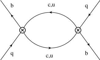
Figure 1: Feynman diagram contributing to $\Gamma_{21}^{q}$ at the LO in QCD.

In terms of the CKM matrix elements $V^{*}_{cb}V_{cq}$ and $V^{*}_{tb}V_{tq}$ (the latter regulates the $M^{q}_{21}$ contribution), the Wilson coefficients $c^{q}_{i}$ and the $\delta^{q}_{1/m_{b}}$ in eq. (15) can be written as

$$\begin{array}[]{l}c^{q}_{i}=(V^{*}_{tb}V_{tq})^{2}\,D^{uu}_{i}+2\,V^{*}_{cb}V_{cq}V^{*}_{tb}V_{tq}\,\left(D^{uu}_{i}-D^{cu}_{i}\right)+(V^{*}_{cb}V_{cq})^{2}\,\left(D^{cc}_{i}+D^{uu}_{i}-2\,D^{cu}_{i}\right)\,,\cr\delta^{q}_{1/m}=(V^{*}_{tb}V_{tq})^{2}\,\delta^{uu\,q}_{1/m}+2\,V^{*}_{cb}V_{cq}V^{*}_{tb}V_{tq}\,\left(\delta^{uu\,q}_{1/m}-\delta^{cu\,q}_{1/m}\right)+(V^{*}_{cb}V_{cq})^{2}\,\left(\delta^{cc\,q}_{1/m}+\delta^{uu\,q}_{1/m}-2\,\delta^{cu\,q}_{1/m}\right)\end{array}$$ (17)

where the labels $cc,\,cu$ and $uu$ denote the intermediate quark pair contributing to $\Gamma_{21}^{q}$, see the diagram in fig. 1. The unitarity of the CKM matrix has been used to drop out $V^{*}_{ub}V_{uq}=-V^{*}_{cb}V_{cq}-V^{*}_{tb}V_{tq}$.

In this paper, we compute the QCD NLO corrections to $D^{cc}_{i}\,,D^{cu}_{i}\,,D^{uu}_{i}$ taking into account the finite value of the charm quark mass. Our results are collected in appendix A. The results for $D^{cc}_{i}$ are in agreement with a previous calculation [11]. The functions $D^{cu}_{i}\,,D^{uu}_{i}$ have been previously estimated [12] taking the limit of a massless charm quark of $D^{cc}_{i}$. As stressed in the introduction, this approximation is not fully satisfactory, in particular if one wants to investigate the dependence on the phase of the mixing in $\Delta\Gamma_{d}/\Gamma_{d}$ and the $|q/p|$ parameters.

As far as the $1/m$ contributions are concerned, $\delta^{cc\,q}_{1/m}$ and $\delta^{cu\,q}_{1/m}$, $\delta^{uu\,q}_{1/m}$ in eq. (17) have been calculated in [10] and [12] respectively. We have repeated the calculation by expanding in $1/m_{b}$ the relevant Feynman diagrams and found agreement with the previous results.

3 Calculation of the Wilson coefficients for $\Gamma^{q}_{21}$

In this section, we discuss the basic ingredients of the calculation of the NLO QCD corrections to $\Gamma^{q}_{21}$, at the leading power in $1/m_{b}$, and of the calculation of the $1/m_{b}$ corrections at the LO in QCD. We refer the interested reader to refs. [6, 8] for further details on the NLO calculation.

3.1 NLO QCD corrections at the leading order in $1/m_{b}$

Although at the leading order in $1/m_{b}$ the heavy quark expansion of the width difference could be expressed directly in terms of QCD operators, we found it easier to perform first the expansion in terms of HQET operators and then translating the results into QCD, once IR divergences are canceled out.

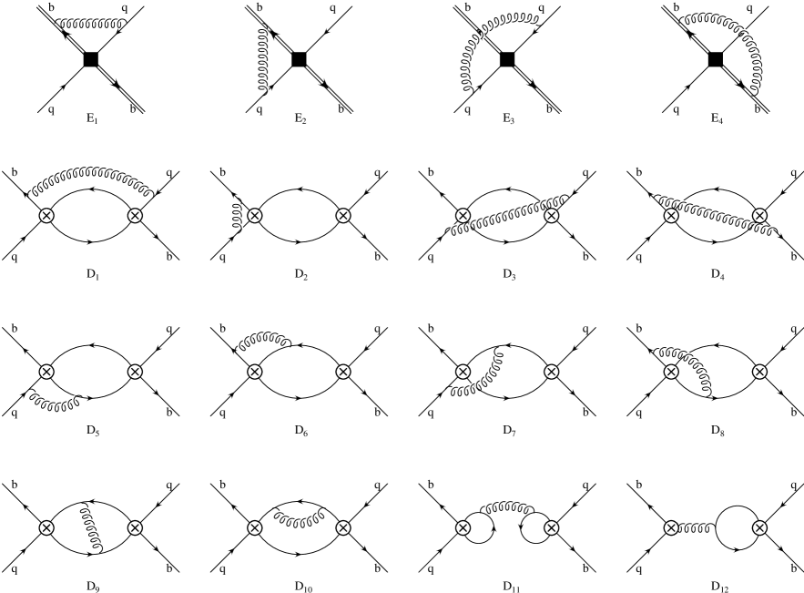
Figure 2: Feynman diagrams which contribute at the NLO to the matrix element of the transition operator ${\cal T}$, both in the full theory ($D_{i}$) and in the effective theory ($E_{i}$). The diagrams obtained from $E_{1},\,E_{2},\,D_{1},\,D_{2},\,D_{5},\,D_{6},\,D_{7},\,D_{8},\,D_{10}$ and $D_{12}$ by a $180^{o}$ rotation (keeping fixed the flavour of the internal lines), as well as those containing the self-energy one-loop corrections to the external fields are not shown.

In order to compute the Wilson coefficients of the $\Delta B=2$ operators at the NLO, we have evaluated in QCD the imaginary part of the diagrams $D_{i}$ shown in fig. 2 (full theory) and in the HQET the diagrams $E_{i}$ (effective theory). The external quark states have been taken on-shell and all quark masses, except $m_{b}$ and $m_{c}$, have been neglected. More specifically, we have chosen the heavy quark momenta $p_{b}^{2}=m_{b}^{2}$ in QCD and $k_{b}=0$ in the HQET while, for the external light quarks, $p_{q}=0$ in both cases. We have performed the calculation in a generic covariant gauge, in order to check the gauge independence of the final results. Two-loop integrals have been reduced to a set of independent master integrals by using the TARCER package [19].

IR and UV divergences have been regularized by $D$-dimensional regularization with anticommuting $\gamma_{5}$ (NDR). As discussed in detail in ref. [6], in the presence of dimensionally-regularized IR divergences the matching must be consistently performed in $D$ dimensions, including the contribution of (renormalized) evanescent operators [20]. All the evanescent operators entering the matching procedure are collected in appendix B.

As a check of the perturbative calculation, we have verified that our results for the Wilson coefficients satisfy the following requirements:

• gauge invariance: the coefficient functions in the $\overline{\rm{MS}}$ scheme are explicitly gauge-invariant. The same is true for the full and the effective amplitudes separately;

• renormalization-scale dependence: the coefficient functions have the correct logarithmic scale dependence as predicted by the LO anomalous dimensions of the $\Delta B=2$ and $\Delta B=1$ operators;

• renormalization-scheme dependence: we performed the calculation in two different $\mbox{NDR-}\overline{\rm{MS}}$ schemes for the $\Delta B=2$ operators (see appendix B and refs. [11, 21] for a detailed definition of these schemes) and verified that the NLO Wilson coefficients obtained in the two cases are related by the appropriate matching matrix;

• IR divergences: the coefficient functions are infrared finite;

• IR regularization: in the limit $m_{c}\to 0$, we have also checked that a calculation using the gluon mass as IR regulator gives the same results. In this case, the matrix elements of the renormalized evanescent operators vanish and hence these operators do not give contribution in the matching procedure;

• comparison with the results in [11]: our results for $D^{cc}_{i}$ defined in eq. (17) and given in appendix A agree with those obtained in ref. [11].

The $\Delta B=2$ effective theory is derived from the double insertion of the $\Delta B=1$ effective Hamiltonian. Therefore, the coefficient functions $D^{cc}_{k}$, $D^{cu}_{k}$ and $D^{uu}_{k}$ of the $\Delta B=2$ effective theory depend quadratically on the coefficient functions $C_{i}$ of the $\Delta B=1$ effective Hamiltonian. The dependence on the renormalization scheme and on the scale $\mu_{1}$ of the $\Delta B=1$ operators actually cancels order by order in perturbation theory against the corresponding dependence of the $\Delta B=1$ Wilson coefficients $C_{i}$. Therefore, the coefficient functions $c^{q}_{k}$ only depend on the renormalization scheme and on the scale $\mu_{2}$ of the $\Delta B=2$ operators.

	LO	${\cal O}(\alpha_{s})$	NLO	${\cal O}(\alpha_{s})$	NLO
		$\alpha_{s}m_{c}=0$
$D^{uu}_{1}$	0.260	-0.123	0.174	-0.123	0.174
$D^{uu}_{1}-D^{cu}_{1}$	0.103	0	0.105	-0.034	0.072
$D^{cc}_{1}+D^{uu}_{1}-2\,D^{cu}_{1}$	0.004	0	0.004	-0.005	-0.001
$D^{uu}_{2}$	-1.56	0.44	-1.00	0.44	-1.00
$D^{uu}_{2}-D^{cu}_{2}$	-0.035	0	-0.033	0.012	-0.022
$D^{cc}_{2}+D^{uu}_{2}-2\,D^{cu}_{2}$	0.016	0	0.015	-0.014	0.001

Table 1: Values of the Wilson coefficients defined in eq. (17) computed at the reference scales $\mu_{1}=\mu_{2}=m_{b}=4.75$ GeV. The LO (first column) and NLO (third and fifth column) coefficients are shown together with the pure ${\cal O}(\alpha_{s})$ contribution (second and fourth column). The results given in the second and third column are those obtained by neglecting the ${\cal O}(\alpha_{s}m_{c})$ corrections.

The analytical expressions of the Wilson coefficients are collected in appendix A. For illustrative purposes, the corresponding numerical values, at the reference scales $\mu_{1}=\mu_{2}=m_{b}$ are presented in table 1. In this table, the LO and NLO coefficients are shown together with the pure ${\cal O}(\alpha_{s})$ contribution, both in the case of a finite charm quark mass and in the charm massless limit . The NLO coefficients refer to the QCD operators renormalized in the $\mbox{NDR-}\overline{\rm{MS}}$ scheme of ref. [11]. In order to obtain the numerical results we used the central values of the input parameters given in table 2.

By looking at the results shown in table 1, we see that the NLO corrections are large and the effect of charm contributions is crucial to estimate accurately all the terms in eq. (17).

3.2 $1/m_{b}$ Corrections to $\Gamma_{21}^{q}$ at the LO in QCD

In order to compute the $1/m_{b}$ correction at the LO in QCD, the imaginary part of the diagrams in fig. 1 have been evaluated between on-shell quark states and expanded in the quark momenta . The result of the full theory has been then matched at ${\cal O}(1/m_{b})$ onto the following independent set of QCD operators,

$$\begin{array}[]{ll}R^{q}_{1}={\displaystyle{m_{q}\over m_{b}}}(\bar{b}_{i}q_{i})_{S-P}(\bar{b}_{j}q_{j})_{S+P}\,,&\!\!\!\!\!\!\!R^{q}_{2}={\displaystyle{1\over m^{2}_{b}}}(\bar{b}_{i}{\overleftarrow{D}}_{\!\rho}\gamma^{\mu}(1-\gamma_{5})D^{\rho}q_{i})(\bar{b}_{j}\gamma_{\mu}(1-\gamma_{5})q_{j})\,,\cr R^{q}_{3}={\displaystyle{1\over m^{2}_{b}}}(\bar{b}_{i}{\overleftarrow{D}}_{\!\rho}(1-\gamma_{5})D^{\rho}q_{i})(\bar{b}_{j}(1-\gamma_{5})q_{j})\,,&R^{q}_{4}={\displaystyle{1\over m_{b}}}(\bar{b}_{i}(1-\gamma_{5})iD_{\mu}q_{i})(\bar{b}_{j}\gamma^{\mu}(1-\gamma_{5})q_{j})\,.\end{array}$$ (18)

Since derivatives acting on $b$ fields scale as $m_{b}$, the above operators are manifestly of order $1/m_{b}$. The results for the $1/m_{b}$ terms defined in eq. (17) read

$$\delta^{cc\,q}_{1/m} = \sqrt{1-4\,z}\,((1+2z)\left[K_{2}\,(\langle R^{q}_{2}\rangle+2\,\langle R^{q}_{4}\rangle)-2\,K_{1}\,(\langle R^{q}_{1}\rangle+\langle R^{q}_{2}\rangle)\right]$$

$$- {\displaystyle{12\,z^{2}\over 1-4\,z}}\left[K_{1}\,(\langle R^{q}_{2}\rangle+2\,\langle R^{q}_{3}\rangle)+2\,K_{2}\,\langle R^{q}_{3}\rangle\right])\,,$$

$$\delta^{cu\,q}_{1/m} = \left(1-z\right)^{2}((1+2z)\left[K_{2}\,(\langle R^{q}_{2}\rangle+2\,\langle R^{q}_{4}\rangle)-2\,K_{1}\,(\langle R^{q}_{1}\rangle+\langle R^{q}_{2}\rangle)\right]$$

$$- {\displaystyle{6\,z^{2}\over(1-z)}}(K_{1}\,(\langle R^{q}_{2}\rangle+2\,\langle R^{q}_{3}\rangle)+2\,K_{2}\,\langle R^{q}_{3}\rangle))\,,$$

$$\delta^{uu\,q}_{1/m} = \left[K_{2}\,(\langle R^{q}_{2}\rangle+2\,\langle R^{q}_{4}\rangle)-2\,K_{1}\,(\langle R^{q}_{1}\rangle+\langle R^{q}_{2}\rangle)\right]\,,$$

where $K_{1}$ and $K_{2}$ are related to the $\Delta B=1$ coefficients, $K_{1}=3\,C^{2}_{1}+2\,C_{1}\,C_{2}$ and $K_{2}=C^{2}_{2}$, and $z=(m_{c}/m_{b})^{2}$. Our results agree with previous calculations [10, 12] .

4 Width differences and CP violation parameters in $B_{q}-\overline{B}_{q}$ mixing

In this section we present the theoretical estimates for the quantities of interest in this paper: the width differences $\Delta\Gamma_{d}/\Gamma_{d}$ and $\Delta\Gamma_{s}/\Gamma_{s}$ and the CP violation parameters $|(q/p)_{d}|$ and $|(q/p)_{s}|$.

Our estimates neglect terms of ${\cal O}(\alpha_{s}^{2})$, ${\cal O}(\alpha_{s}\,(\Lambda_{QCD}/m_{b}))$ and ${\cal O}((\Lambda_{QCD}/m_{b})^{2})$, whereas the charm quark mass contributions have been fully taken into account. For the relevant hadronic matrix elements we have used the lattice determination of ref. [13].

In eq. (10), the width difference $\Delta\Gamma_{q}$ and the parameter $|(q/p)_{q}|$ for neutral $B$ mesons are expressed in terms of the real and the imaginary part of $\Gamma^{q}_{21}/M^{q}_{21}$ respectively. Taking into account the expressions obtained in eq. (11) for $M^{q}_{21}$ and eqs. (15)-(17) for $\Gamma^{q}_{21}$, we can write

$$\Delta\Gamma_{q} = {\displaystyle{\Delta m_{q}\,{\cal K}\over\langle\overline{B}_{q}|{\cal O}^{q}_{1}|B_{q}\rangle}}\times$$ (20)

$$\left(\mathop{\displaystyle\sum}\limits_{i=1,2}\langle\overline{B}_{q}|{\cal O}^{q}_{i}|B_{q}\rangle\left[D^{uu}_{i}+{\displaystyle{\cos 2\beta_{q}\over R^{2}_{t\,q}}}\,\left(D^{cc}_{i}+D^{uu}_{i}-2\,D^{cu}_{i}\right)-2\,{\displaystyle{\cos\beta_{q}\over R_{t\,q}}}\,\left(D^{uu}_{i}-D^{cu}_{i}\right)\right]\right.$$

$$+\left.\left[\delta^{uu\,q}_{1/m}+{\displaystyle{\cos 2\beta_{q}\over R^{2}_{t\,q}}}\,\left(\delta^{cc\,q}_{1/m}+\delta^{uu\,q}_{1/m}-2\,\delta^{cu\,q}_{1/m}\right)-2\,{\displaystyle{\cos\beta_{q}\over R_{t\,q}}}\,\left(\delta^{uu\,q}_{1/m}-\delta^{cu\,q}_{1/m}\right)\right]\right)\,,$$

$$\left|\left({\displaystyle{q\over p}}\right)_{q}\right|-1 = -{\displaystyle{{\cal K}\over 2\,\langle\overline{B}_{q}|{\cal O}^{q}_{1}|B_{q}\rangle}}\times$$ (21)

$$\left(\mathop{\displaystyle\sum}\limits_{i=1,2}\langle\overline{B}_{q}|{\cal O}^{q}_{i}|B_{q}\rangle\left[{\displaystyle{\sin 2\beta_{q}\over R^{2}_{t\,q}}}\,\left(D^{cc}_{i}+D^{uu}_{i}-2\,D^{cu}_{i}\right)-2\,{\displaystyle{\sin\beta_{q}\over R_{t\,q}}}\,\left(D^{uu}_{i}-D^{cu}_{i}\right)\right]\right.$$

$$+\left.\left[{\displaystyle{\sin 2\beta_{q}\over R^{2}_{t\,q}}}\,\left(\delta^{cc\,q}_{1/m}+\delta^{uu\,q}_{1/m}-2\,\delta^{cu\,q}_{1/m}\right)-2\,{\displaystyle{\sin\beta_{q}\over R_{t\,q}}}\,\left(\delta^{uu\,q}_{1/m}-\delta^{cu\,q}_{1/m}\right)\right]\right)\,.$$

The two operators entering these expansions at the leading order, ${\cal O}^{q}_{1}$ and ${\cal O}^{q}_{2}$, are defined in eq. (16). The coefficient ${\cal K}$ is given by ${\cal K}=4\pi m_{b}^{2}/(3M_{W}^{2}\eta_{B}S_{0}(x_{t}))$. In addition we have used

$$V^{*}_{cb}V_{cq}/(V^{*}_{tb}V_{tq})=-e^{i\beta_{q}}/R_{t\,q}\,.$$ (22)

$\beta_{d}$ and $R_{t\,d}$ are the usual angle $\beta$ and the side $R_{t}$ of the unitarity triangle respectively, whereas $\beta_{s}$ and $R_{t\,s}$ parameterize the Cabibbo-suppressed contributions to the $B_{s}$ system. For completeness, we give their expansion in terms of the parameters of CKM matrix, up to and including ${\cal O}(\lambda^{4})$ terms. They read

$$\begin{array}[]{l l}R_{td}=\sqrt{(1-\bar{\rho})^{2}+\bar{\eta}^{2}}\,,&\sin\beta_{d}=\bar{\eta}/R_{td}\,,\cr R_{ts}=1+\lambda^{2}\bar{\rho}+\frac{1}{2}\lambda^{4}(2\bar{\rho}+\bar{\eta}^{2})\,,&\sin\beta_{s}=-\lambda^{2}\bar{\eta}\left[1+\lambda^{2}\left(1-\bar{\rho}\right)\right]\,.\end{array}$$ (23)

The Cabibbo-suppressed contributions are practically irrelevant for $\Delta\Gamma_{s}$ so that, to an excellent approximation, one can put $\beta_{s}=0$ and $R_{t\,s}=1$ in eq. (20) to obtain

$$\Delta\Gamma_{s} = {\displaystyle{\Delta m_{s}\,{\cal K}\over\langle\overline{B}_{s}|{\cal O}^{s}_{1}|B_{s}\rangle}}\,\left(\mathop{\displaystyle\sum}\limits_{i=1,2}\langle\overline{B}_{s}|{\cal O}^{s}_{i}|B_{s}\rangle D^{cc}_{i}+\delta^{cc\,s}_{1/m}+{\cal O}(\lambda^{2})\right)\,.$$ (24)

The contributions neglected in the previous equation, however, give rise to the CP violation effects in the $B_{s}-\overline{B}_{s}$ mixing, which are accounted for by the deviation of the parameter $|(q/p)_{s}|$ from unity. Using $\beta_{s}=0$ and $R_{t\,s}=1$ in eq. (21) gives in fact $|(q/p)_{s}|=1$.

For the matrix elements entering our calculation (see eqs. (16) and (18)), we use the following parameterization

$$\begin{array}[]{ll}\langle\overline{B}_{q}|{\cal O}^{q}_{1}|B_{q}\rangle={\displaystyle{8\over 3}}\,f_{B_{q}}^{2}M^{2}_{B_{q}}\,B^{q}_{1}\,,&\langle\overline{B}_{q}|{\cal O}^{q}_{2}|B_{q}\rangle=-{\displaystyle{5\over 3}}\,{\displaystyle{f_{B_{q}}^{2}M^{4}_{B_{q}}\over(m_{b}+m_{q})^{2}}}\,B^{q}_{2}\,,\cr\langle\overline{B}_{q}|R^{q}_{1}|B_{q}\rangle={\displaystyle{7\over 3}}\,{\displaystyle{m_{q}\over m_{b}}}\,f_{B_{q}}^{2}M_{B_{q}}^{2}\,B^{q}_{R_{1}},&\langle\overline{B}_{q}|R^{q}_{2}|B_{q}\rangle=-{\displaystyle{2\over 3}}\,f_{B_{q}}^{2}M_{B_{q}}^{2}\left({\displaystyle{M_{B_{q}}^{2}\over m_{b}^{2}}}-1\right)\,B^{q}_{R_{2}}\,,\cr\langle\overline{B}_{q}|R^{q}_{3}|B_{q}\rangle={\displaystyle{7\over 6}}\,f_{B_{q}}^{2}M_{B_{q}}^{2}\left({\displaystyle{M_{B_{q}}^{2}\over m_{b}^{2}}}-1\right)\,B^{q}_{R_{3}}\,,&\langle\overline{B}_{q}|R^{q}_{4}|B_{q}\rangle=-f_{B_{q}}^{2}M_{B_{q}}^{2}\left({\displaystyle{M_{B_{q}}^{2}\over m_{b}^{2}}}-1\right)\,B^{q}_{R_{4}}\,.\cr\end{array}$$ (25)

Among these $B$-parameters, $B^{q}_{1}$ and $B^{q}_{2}$ are the most widely studied and well known in lattice QCD [13], [23]-[29]. In this paper we use the results of ref. [13], in which the complete set of $\Delta B=2$, dimension-six, four-fermion operators has been determined in the quenched approximation of QCD. For $B^{q}_{1}$ and $B^{q}_{2}$, the results of [13] are in very good agreement with those obtained in [24, 25] by using the lattice NRQCD approach. In addition, it has been shown in refs. [28, 29] that the effect of the quenching approximation for these quantities is practically irrelevant. Thus, the systematic uncertainties in the present lattice estimates of $B^{q}_{1}$ and $B^{q}_{2}$ are quite under control.

To our knowledge, the matrix elements of the operators $R^{q}_{i}$ defined in eq. (25), entering the $1/m_{b}$ corrections, have been only estimated so far in the VSA. Using the complete set of operator matrix elements calculated in [13], however, two of the four independent parameters $B^{q}_{R_{i}}$ can be also evaluated. Besides the operators ${\cal O}^{q}_{1,2}$, the complete basis studied in [13] includes

$${\cal O}^{q}_{3}=(\bar{b}_{i}q_{j})_{S-P}(\bar{b}_{j}q_{i})_{S-P}\,,\quad{\cal O}^{q}_{4}=(\bar{b}_{i}q_{i})_{S-P}(\bar{b}_{j}q_{j})_{S+P}\,,\quad{\cal O}^{q}_{5}=(\bar{b}_{i}q_{j})_{S-P}(\bar{b}_{j}q_{i})_{S+P}\,,$$ (26)

whose matrix elements are parametrized as

$$\langle\overline{B}_{q}|{\cal O}^{q}_{3}|B_{q}\rangle = {1\over 3}\,\left({m_{B_{q}}\over m_{b}+m_{q}}\right)^{2}m_{B_{q}}^{2}f_{B_{q}}^{2}B^{q}_{3}\,,$$

$$\langle\overline{B}_{q}|{\cal O}^{q}_{4}|B_{q}\rangle = 2\,\left({m_{B_{q}}\over m_{b}+m_{q}}\right)^{2}m_{B_{q}}^{2}f_{B_{q}}^{2}B^{q}_{4}\,,$$ (27)

$$\langle\overline{B}_{q}|{\cal O}^{q}_{5}|B_{q}\rangle = {2\over 3}\,\left({m_{B_{q}}\over m_{b}+m_{q}}\right)^{2}m_{B_{q}}^{2}f_{B_{q}}^{2}B^{q}_{5}\,.$$

We then notice that the operator $R^{q}_{1}$ defined in eq. (18) is trivially related to ${\cal O}^{q}_{4}$,

$$R^{q}_{1}={\displaystyle{m_{q}\over m_{b}}}\,{\cal O}^{q}_{4}\,.$$ (28)

In addition, by using the Fierz identities and the equations of motion, the operator $R^{q}_{4}$ can be expressed as [10]

$$2R^{q}_{4}={\cal O}^{q}_{3}+{\cal O}^{q}_{1}/2+{\cal O}^{q}_{2}-2{\displaystyle{m_{q}\over m_{b}}}\,{\cal O}^{q}_{5}+R^{q}_{2}\,.$$ (29)

Thus, eqs. (28) and (29) can be used to get rid of the two parameters $B^{q}_{R_{1}}$ and $B^{q}_{R_{4}}$.

The values of the $B$-parameters obtained in ref. [13] and used in our calculation are collected in table 2. Concerning the unknown matrix elements of the operators $R^{q}_{2}$ and $R^{q}_{3}$, they have been estimated in the VSA and we have included a 30% of relative error to account for the corresponding systematic uncertainty .

$m_{b}$ = $4.75\pm 0.11$ GeV	$m_{c}/m_{b}$ = $0.30\pm 0.02$
${\overline{m}}_{t}({\overline{m}}_{t})=165.0\pm 5.0$ GeV	${\overline{m}}_{s}({\overline{m}}_{b})=87\pm 21$ MeV
$M_{W}=80.41$ GeV	$\Delta m_{d}$ = $0.502\pm 0.006$ $\rm{ps}^{-1}$
$\tau(B_{s})=1.461\pm 0.057$ ps	$\tau(B_{d})=1.540\pm 0.014$ ps
$M_{B_{d}}=5.279$ GeV	$M_{B_{s}}=5.369$ GeV
$\eta_{b}(m_{b})=0.85\pm 0.02$	$\xi=1.24\pm 0.04$
$\lambda=0.2240\pm 0.0036$	$\alpha_{s}(m_{Z})=0.118$
$\bar{\rho}=0.162\pm 0.046$	$\bar{\eta}=0.347\pm 0.027$
$B_{1}^{s}$ = $0.87\pm 0.05$	$B_{1}^{s}/B_{1}^{d}$ = $0.99\pm 0.02$
$B_{2}^{s}$ = $0.84\pm 0.04$	$B_{2}^{s}/B_{2}^{d}$ = $1.01\pm 0.02$
$B_{3}^{s}$ = $0.91\pm 0.08$	$B_{3}^{s}/B_{3}^{d}$ = $1.01\pm 0.03$
$B_{4}^{s}$ = $1.16\pm 0.07$	$B_{4}^{s}/B_{4}^{d}$ = $1.01\pm 0.02$
$B_{5}^{s}$ = $1.75\pm 0.20$	$B_{5}^{s}/B_{5}^{d}$ = $1.01\pm 0.03$

Table 2: Central values and standard deviations of the input parameters used to obtain the theoretical estimates of the width differences and of the CP violation parameters. When the error is not quoted, the parameter has been kept fixed in the numerical analysis. The values of $m_{b}$ and $m_{c}$ refer to the pole masses, while ${\overline{m}}_{s}$ and ${\overline{m}}_{t}$ are the masses in the $\mbox{NDR-}\overline{\rm{MS}}$ scheme. The $B$-parameters are renormalized in the $\mbox{NDR-}\overline{\rm{MS}}$ scheme at the scale $m_{b}$. The definition of the renormalization scheme can be found in [11] for $B_{1}^{q}$, $B_{2}^{q}$ and $B_{3}^{q}$ and in [20] for $B_{4}^{q}$ and $B_{5}^{q}$, see also appendix B.

In order to obtain the theoretical predictions presented in this paper, we have performed a Bayesian statistical analysis by implementing a simple Monte Carlo calculation. The input parameters have been extracted with flat distributions, by assuming the central values and standard deviations given in table 2.

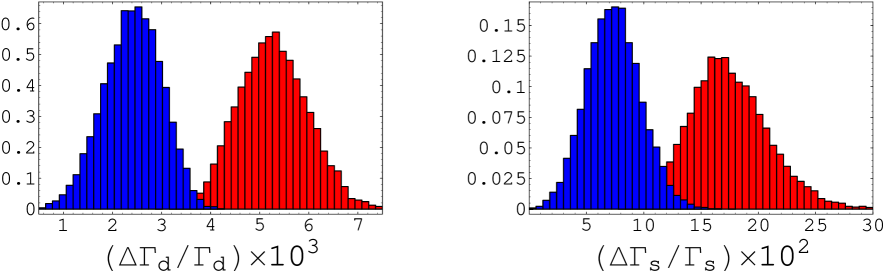
Figure 3: Theoretical distributions for the width differences in the $B_{d}$ and $B_{s}$ systems. The predictions are shown at both the LO (light/red) and NLO (dark/blue).

4.1 Width differences: $\Delta\Gamma_{d}/\Gamma_{d}$, $\Delta\Gamma_{s}/\Gamma_{s}$ and $\Delta\Gamma_{d}/\Delta\Gamma_{s}$

The theoretical predictions for the width differences $\Delta\Gamma_{d}/\Gamma_{d}$ and $\Delta\Gamma_{s}/\Gamma_{s}$, as obtained from eq. (20) as functions of the CKM matrix elements and of the $B$-parameters entering at the LO in $1/m_{b}$, can be expressed as

$$\left(\frac{\Delta\Gamma_{d}}{\Gamma_{d}}\right) = 10^{-3}\,\left[0.96(10)+5.48(34){\displaystyle{B^{d}_{2}\over B^{d}_{1}}}-2.9(1.3){\displaystyle{1\over B^{d}_{1}}}\right.$$ (30)

$$\phantom{10^{-3}}-{\displaystyle{\cos\beta\over R_{t}}}\left(0.80(13)+0.24(7){\displaystyle{B^{d}_{2}\over B^{1}_{d}}}-0.03(6){\displaystyle{1\over B^{d}_{1}}}\right)$$

$$\phantom{10^{-3}}\left.+\frac{\cos 2\beta}{R_{t}^{2}}\left(-0.005(4)-0.007(16)\frac{B^{d}_{2}}{B^{d}_{1}}-0.008(17)\frac{1}{B^{d}_{1}}\right)\right]\,,$$

$$\left(\frac{\Delta\Gamma_{s}}{\Gamma_{s}}\right) = \frac{10^{-2}}{(\lambda\,R_{t})^{2}}\,\left(0.02(2)+0.77(7){\displaystyle{B^{s}_{2}\over B^{s}_{1}}}-0.47(18){\displaystyle{1\over B^{s}_{1}}}\right).$$ (31)

These formulae are one of the main results of this paper. In the above expressions, the terms proportional to $1/B^{q}_{1}$ represent the contributions of the $1/m_{b}$ corrections. Note also that, in order to obtain the prediction for $\Delta\Gamma_{s}/\Gamma_{s}$, the mass difference $\Delta m_{s}$ has been evaluated in terms of $\Delta m_{d}$ by using

$$\Delta m_{s}=\Delta m_{d}\,{\displaystyle{M_{B_{s}}\over M_{B_{d}}}}\,\left|{\displaystyle{V_{ts}\over V_{td}}}\right|^{2}\xi^{2}\,,$$ (32)

where $\xi=\Big{(}f_{B_{s}}\sqrt{B^{s}_{1}}\Big{)}/\Big{(}f_{B_{d}}\sqrt{B^{d}_{1}}\Big{)}$.

The errors on the numerical coefficients presented in eqs. (30) and (31) take into account both the residual NNLO dependence on the renormalization scale of the $\Delta B=1$ operators and the theoretical uncertainties on the various input parameters. To estimate the former, the scale $\mu_{1}$ has been varied in the interval between $m_{b}/2$ and $2m_{b}$. These errors are strongly correlated, since they originate from the theoretical uncertainties on the same set of input parameters. For this reason, they have not been used to derive our final predictions for the width differences. For these predictions, we quote the average and the standard deviation of the corresponding probability distribution functions obtained directly from the Monte Carlo simulation, namely

$$\Delta\Gamma_{d}/\Gamma_{d}=(2.42\pm 0.59)\times 10^{-3}\,,\qquad\Delta\Gamma_{s}/\Gamma_{s}=(7.4\pm 2.4)\times 10^{-2}\,.$$ (33)

The theoretical distributions are shown in fig. 3. Notice that the difference between the NLO and LO distributions is remarkable. The NLO corrections decrease the values of both $\Delta\Gamma_{d}/\Gamma_{d}$ and $\Delta\Gamma_{s}/\Gamma_{s}$ by about a factor two with respect to the LO predictions. We find that the total error on the width differences is dominated by the uncertainty on the $b$-quark mass in the first place, followed closely by the one due to the renormalization scale variation. Other contributions to the error, coming from the ratio $m_{c}/m_{b}$, the $B$- and the CKM-parameters are smaller, though not entirely negligible.

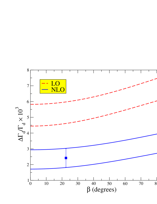
Figure 4: Prediction for $\Delta\Gamma_{d}/\Gamma_{d}$ as a function of $\beta$ as obtained at the LO and NLO. The NLO estimate of $\Delta\Gamma_{d}/\Gamma_{d}$ at the measured value of $\beta$ is also shown.

In fig. 4 we show the dependence of $\Delta\Gamma_{d}/\Gamma_{d}$ on the mixing phase $\beta$ as given in eq. (30). NLO corrections in the limit of vanishing $m_{c}$ just shift the LO curve, while $m_{c}$-dependent terms modify also its profile. In principle, a measurement of $\Delta\Gamma_{d}/\Gamma_{d}$ could allow a determination of $\beta$, but we find that the dependence is so mild that the extracted value would be affected by a very large error.

Another interesting prediction concerns the ratio $\Delta\Gamma_{d}/\Delta\Gamma_{s}$. This quantity is of particular interest, because the uncertainties coming from higher order QCD and $\Lambda_{QCD}/m_{b}$ corrections, as well as those coming from the non-perturbative estimates of the $B$-parameters, are expected to cancel in this ratio to some extent. From our numerical analysis, we obtain the NLO prediction

$$\Delta\Gamma_{d}/\Delta\Gamma_{s}=(3.2\pm 0.8)\times 10^{-2}\,.$$ (34)

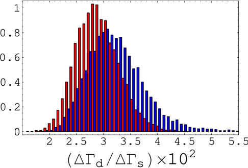
Figure 5: Theoretical distribution for the ratio $\Delta\Gamma_{d}/\Delta\Gamma_{s}$ as obtained at both the LO (light/red) and NLO (dark/blue).

The corresponding theoretical distributions at the LO and NLO are shown in fig. 5. As can be seen from the plot, this quantity is practically unaffected by the NLO corrections.

4.2 CP Violation parameters: $|(q/p)_{d}|$ and $|(q/p)_{s}|$

CP violation in the mixing shows up only for a non-vanishing value of the charm quark mass, as can be explicitly verified from the expression of $|(q/p)_{q}|$ in eq. (21). In addition, it is apparent from eq. (21) that $|(q/p)_{s}|-1$ is suppressed with respect to $|(q/p)_{d}|-1$ by a factor $\sin\beta_{s}\sim\lambda^{2}$.

For the parameters $|(q/p)_{d}|$ and $|(q/p)_{s}|$, expressed in terms of the CKM matrix elements and the $B$-parameters $B^{q}_{1},\,B^{q}_{2}$, we obtain the expression

$$\left|\left({\displaystyle{q\over p}}\right)_{q}\right|-1 = 10^{-4}\left[{\displaystyle{\sin\beta_{q}\over R_{tq}}}\left(5.19(84)+1.57(47){\displaystyle{B^{q}_{2}\over B^{q}_{1}}}-0.22(39){\displaystyle{1\over B^{q}_{1}}}\right)\right.$$ (35)

$$\phantom{10^{-4}}\left.+\frac{\sin 2\beta_{q}}{R_{tq}^{2}}\left(0.04(3)+0.04(10)\frac{B^{q}_{2}}{B^{q}_{1}}+0.05(11)\frac{1}{B^{q}_{1}}\right)\right]\,,$$

where $q=d,s$.

By using the values of the CKM and $B$-parameters given in table 2 we obtain from the Monte Carlo analysis the final predictions

$$\left|\left({\displaystyle{q\over p}}\right)_{d}\right|-1=(2.96\pm 0.67)\times 10^{-4}\quad,\quad\left|\left({\displaystyle{q\over p}}\right)_{s}\right|-1=-(1.28\pm 0.27)\times 10^{-5}\,.$$ (36)

The theoretical distributions for these quantities are shown in fig. 6 both at the LO and NLO.

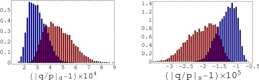
Figure 6: Theoretical distributions for $|(q/p)_{q}|-1$ in the $B_{d}$ and $B_{s}$ systems. The predictions are shown at the LO (light/red) and NLO (dark/blue).

One can see that the effect of the NLO corrections turns out to be important also for these quantities. The error on $|(q/p)_{q}|-1$ is largely dominated by the uncertainties on $m_{c}/m_{b}$ and on the CKM parameters. We note in particular that the dependence on the $B$-parameters is practically negligible, making these predictions free from hadronic uncertainties.

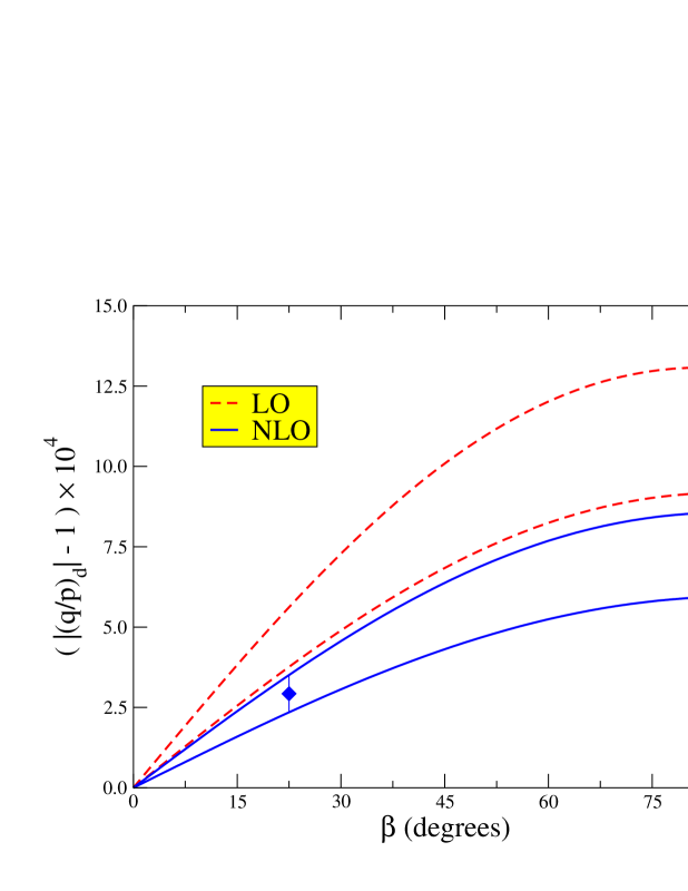
Figure 7: Prediction for the CP violation parameter $|(q/p)_{d}|-1$ as a function of $\beta$ as obtained at both the LO and NLO. The NLO estimate of $|(q/p)_{d}|-1$ at the measured value of $\beta$ is also shown.

Finally, we show in fig. 7 the LO and NLO predictions for $|(q/p)_{d}|-1$ as functions of $\beta$. In this case, NLO corrections without charm mass leave the LO result practically unchanged, while the $m_{c}$-dependent terms give a sizable contribution. The dependence on $\beta$ is quite strong, allowing for a determination of the mixing angle once $|(q/p)_{d}|$ will be measured.

5 Conclusions

The main result of this paper is the NLO QCD calculation of the Wilson coefficients entering the heavy quark expansion of $\Gamma_{21}^{d}$ and $\Gamma_{21}^{s}$, including the effects of a non-vanishing charm quark mass. For $\Gamma_{21}^{s}$ we find agreement with a previous result [11]. Using our results, we improve the theoretical predictions for different observables in the neutral $B$-meson systems, namely the width differences $\Delta\Gamma_{d}/\Gamma_{d}$ and $\Delta\Gamma_{s}/\Gamma_{s}$ and the CP violation parameters $|(q/p)_{d}|$ and $|(q/p)_{s}|$.

Using formulae including the NLO $\alpha_{s}$ corrections at the lowest order in the $1/m_{b}$ expansion and the first power corrections at the LO in $\alpha_{s}$, we find

$$\frac{\Delta\Gamma_{d}}{\Gamma_{d}}=(2.42\pm 0.59)\times 10^{-3}\,,\quad\frac{\Delta\Gamma_{s}}{\Gamma_{s}}=(7.4\pm 2.4)\times 10^{-2}\,,\quad\frac{\Delta\Gamma_{d}}{\Delta\Gamma_{s}}=(3.2\pm 0.8)\times 10^{-2}\,,$$

$$\left|\left(q/p\right)_{d}\right|-1=(2.96\pm 0.67)\times 10^{-4}\,,\quad\left|\left(q/p\right)_{s}\right|-1=-(1.28\pm 0.27)\times 10^{-5}\,.$$ (37)

NLO QCD corrections are in general important for theoretical consistency and give sizable contributions to the Wilson coefficients considered in this paper. We find that the charm quark mass effects at NLO are numerically important, in particular for $|(q/p)_{q}|$, and should be included in the phenomenological analyses.

Note added

Just before this paper was finalized, a paper by Beneke et al. on the same subject was submitted to the e-print archive [34]. Comparing the results, we found that the NLO contribution to the Wilson coefficients $D_{k}^{cu}$ of eqs. (17) and (38) differ from the ones given in eq. (25) of ref. [34]. Had we assumed that the diagrams $D_{6}$, $D_{7}$ and $D_{8}$ in fig. 2 were equal to the corresponding “rotated” ones (i.e. those diagrams where the gluon is attached to the other external quark leg with the same flavour and to the other virtual quark line), we would have obtained the result of ref. [34]. However this assumption, which is correct when the two virtual lines correspond to the same flavour, does not hold when the two quarks are different. This may explain the origin of the discrepancy.

Appendix A: Analytical Results for the $\Delta B=2$ Wilson Coefficients

In this appendix we collect the analytical expressions of the Wilson coefficients, both at the LO and NLO. The LO coefficients have been computed in refs. [10, 12] and are given here for completeness.

The coefficient functions $D^{uu}_{k}$, $D^{cu}_{k}$ and $D^{cc}_{k}$ defined in eq.(17) depend quadratically on the coefficient functions $C_{i}$ of the $\Delta B=1$ effective Hamiltonian and can be written as

$$D^{uu}_{k}(\mu_{2}) = \mathop{\displaystyle\sum}_{i,j=1,2}C_{i}(\mu_{1})\,C_{j}(\mu_{1})F^{uu}_{k,ij}(\mu_{1},\mu_{2})+\frac{\alpha_{s}}{4\pi}\,C_{2}(\mu_{1})^{2}P^{uu}_{k,22}(\mu_{1},\mu_{2})$$

$$+ 2\,\frac{\alpha_{s}}{4\pi}\,C_{2}\,C_{8G}P^{u}_{k,28}+2\,\mathop{\displaystyle\sum}_{i=1,2}\mathop{\displaystyle\sum}_{r=3,6}C_{i}\,C_{r}P^{u}_{k,ir}\,,$$

$$D^{cu}_{k}(\mu_{2}) = \sum_{i,j=1,2}C_{i}(\mu_{1})\,C_{j}(\mu_{1})\,F^{cu}_{k,ij}(\mu_{1},\mu_{2})+\frac{\alpha_{s}}{4\pi}\,C_{2}(\mu_{1})^{2}P^{cu}_{k,22}(\mu_{1},\mu_{2})$$

$$+ \frac{\alpha_{s}}{4\pi}\,C_{2}\,C_{8G}\left(P^{c}_{k,28}+P^{u}_{k,28}\right)+\,\mathop{\displaystyle\sum}_{i=1,2}\mathop{\displaystyle\sum}_{r=3,6}C_{i}\,C_{r}\left(P^{c}_{k,ir}+P^{u}_{k,ir}\right)\,,$$

$$D^{cc}_{k}(\mu_{2}) = \mathop{\displaystyle\sum}_{i,j=1,2}C_{i}(\mu_{1})\,C_{j}(\mu_{1})F^{cc}_{k,ij}(\mu_{1},\mu_{2})+\frac{\alpha_{s}}{4\pi}\,C_{2}(\mu_{1})^{2}P^{cc}_{k,22}(\mu_{1},\mu_{2})$$ (38)

$$+ 2\,\frac{\alpha_{s}}{4\pi}\,C_{2}\,C_{8G}P^{c}_{k,28}+2\,\mathop{\displaystyle\sum}_{i=1,2}\mathop{\displaystyle\sum}_{r=3,6}C_{i}\,C_{r}P^{c}_{k,ir}\,.$$

The functions $F^{qq^{\prime}}_{k,ij}$ are obtained from the insertion of the operators $Q_{i}$ and $Q_{j}$ in the Feynman diagrams $D_{1}-D_{10}$ of fig. 2, whereas the diagrams $D_{11}$ and $D_{12}$ contribute to the functions $P^{qq^{\prime}}_{k,22}(\mu_{1},\mu_{2})$ and $P^{q}_{k,ij}$ respectively. Contributions with the double insertion of penguin operators have been neglected, since the Wilson coefficients $C_{3}$–$C_{6}$ are numerically small.

We distinguish the leading and next-to-leading contributions in the coefficients $F^{qq^{\prime}}_{k,ij}$ by writing the expansion

$$F^{qq^{\prime}}_{k,ij}=A^{qq^{\prime}}_{k,ij}+\frac{\alpha_{s}}{4\pi}B^{qq^{\prime}}_{k,ij}\,,$$ (39)

where $(qq^{\prime})=\{(uu),(cu),(cc)\}$. Since only the sum of $F^{qq^{\prime}}_{k,12}$ and $F^{qq^{\prime}}_{k,21}$ contributes to eq. (38), we just give in the following the average of the components 12 and 21. Moreover, we do not write explicitly the results for the functions $D^{uu}_{k}$ since they can be obtained by taking the limit $m_{c}\to 0$ of $D^{cc}_{k}$.

In terms of the ratio $z=m_{c}^{2}/m_{b}^{2}$, the LO coefficients $A^{qq^{\prime}}_{k,ij}$ read

$$\begin{array}[]{lll}A^{cu}_{1,11}={\frac{3}{2}}\,\left(2-3\,z+{z^{3}}\right)\,,&A^{cu}_{1,12}=A^{cu}_{1,21}={\frac{1}{2}}\,\left(2-3\,z+{z^{3}}\right)\,,&A^{cu}_{1,22}={\frac{1}{2}}\,{\left(1-z\right)}^{3}\,,\\ A^{cu}_{2,11}=3\,{{\left(1-z\right)}^{2}}\,\left(1+2\,z\right)\,,&A^{cu}_{2,12}=A^{cu}_{2,21}={{\left(1-z\right)}^{2}}\,\left(1+2\,z\right)\,,&A^{cu}_{2,22}=-{{\left(1-z\right)}^{2}}\,\left(1+2\,z\right)\,.\end{array}$$ (40)

$$\begin{array}[]{lll}A^{cc}_{1,11}=3\,{\sqrt{1-4\,z}}\,\left(1-z\right)\,,&A^{cc}_{1,12}={\sqrt{1-4\,z}}\,\left(1-z\right)\,,&A^{cc}_{1,22}={\frac{1}{2}}\,{\left(1-4\,z\right)}^{\frac{3}{2}}\,,\\ A^{cc}_{2,11}=3\,{\sqrt{1-4\,z}}\,\left(1+2\,z\right)\,,&A^{cc}_{2,12}={\sqrt{1-4\,z}}\,\left(1+2\,z\right)\,,&A^{cc}_{2,22}=-{\sqrt{1-4\,z}}\,\left(1+2\,z\right)\,.\end{array}$$ (41)

The NLO results for the coefficients $B^{qq^{\prime}}_{k,ij}$ are presented in the $\mbox{NDR-}\overline{\rm{MS}}$ scheme of ref. [21] for the $\Delta B=1$ operators and the $\mbox{NDR-}\overline{\rm{MS}}$ scheme of ref. [11] for the $\Delta B=2$ operators, in QCD. We find

$$B^{cu}_{1,11} = {\frac{109}{6}}-37\,z+{\frac{3\,{z^{2}}}{2}}+{\frac{52\,{z^{3}}}{3}}+2\,{{\left(1-z\right)}^{2}}\,\left(5+z\right)\,\log x_{2}-4\,{{\left(1-z\right)}^{2}}\,\left(5+7\,z\right)\,\log(1-z)-$$

$$2\,z\,\left(10+14\,z-15\,{z^{2}}\right)\,\log z+8\,\left(2-3\,z+{z^{3}}\right)\,\log(1-z)\,\log z+16\,\left(2-3\,z+{z^{3}}\right)\,\mathrm{Li_{2}}(z)\,,$$

$$B^{cu}_{2,11} = {-\frac{4}{3}\,\left(10-33\,z+54\,{z^{2}}-31\,{z^{3}}\right)}-8\,{{\left(1-z\right)}^{2}}\,\left(4+14\,z-3\,{z^{2}}\right)\,\log(1-z)+$$ (42)

$$8\,z\,\left(2-23\,z+21\,{z^{2}}-3\,{z^{3}}\right)\,\log z-$$

$$16\,{{\left(1-z\right)}^{2}}\,\left(1+2\,z\right)\,\left(2\,\log x_{2}-\log(1-z)\,\log z-2\,\mathrm{Li_{2}}(z)\right)\,,$$

$${\displaystyle{B^{cu}_{1,12}+B^{cu}_{1,21}\over 2}} = {\frac{-502+912\,z-387\,{z^{2}}-23\,{z^{3}}}{36}}-{{\left(1-z\right)}^{2}}\,\left(17+4\,z\right)\,\log x_{1}+\frac{2}{3}\left(1-z\right)^{2}\,\left(5+z\right)\,\log x_{2}-$$

$${\frac{{{\left(1-z\right)}^{2}}}{12\,z}\,\left(2+33\,z+94\,{z^{2}}\right)\,\log(1-z)}-{\frac{z}{12}\left(80+69\,z-126\,{z^{2}}\right)\,\log z}+$$

$${\frac{8}{3}\,\left(2-3\,z+{z^{3}}\right)\,\left(\log(1-z)\,\log z+2\,\mathrm{Li_{2}}(z)\right)}\,,$$

$${\displaystyle{B^{cu}_{2,12}+B^{cu}_{2,21}\over 2}} = {\frac{-130+93\,z+144\,{z^{2}}-107\,{z^{3}}}{9}}-{\frac{2\,{{\left(1-z\right)}^{2}}}{3\,z}\,\left(1+15\,z+47\,{z^{2}}-12\,{z^{3}}\right)\,\log(1-z)}+$$ (43)

$${\frac{2}{3}\,z\,\left(8-93\,z+87\,{z^{2}}-12\,{z^{3}}\right)\,\log z}-$$

$${\frac{8}{3}\,{{\left(1-z\right)}^{2}}\,\left(1+2\,z\right)\,\left(3\,\log x_{1}+4\,\log x_{2}-2\,\log(1-z)\,\log z-4\,\mathrm{Li_{2}}(z)\right)}\,,$$

$$B^{cu}_{1,22} = {-\frac{{{\pi}^{2}}}{3}\,\left(1-5\,z+4\,{z^{2}}\right)}+{\frac{-136-159\,z+738\,{z^{2}}-443\,{z^{3}}}{18}}-2\,{{\left(1-z\right)}^{2}}\,\left(5+4\,z\right)\,\log x_{1}+$$

$${\frac{2}{3}\,{{\left(1-z\right)}^{2}}\,\left(4-z\right)\,\log x_{2}}+{\frac{{{\left(1-z\right)}^{2}}}{6\,z}\,\left(7+32\,{z^{2}}+3\,{z^{3}}\right)\,\log(1-z)}-$$

$${\frac{z}{6}\,\left(62-39\,z-30\,{z^{2}}+3\,{z^{3}}\right)\,\log z}+{\frac{\left(5-3\,z-18\,{z^{2}}+16\,{z^{3}}\right)}{3}\,\left(\log(1-z)\,\log z+2\,\mathrm{Li_{2}}(z)\right)}\,,$$

$$B^{cu}_{2,22} = {\frac{8}{3}\,{{\pi}^{2}}\,\left(1+z-2\,{z^{2}}\right)}-{\frac{28}{9}\,\left(5+3\,z-27\,{z^{2}}+19\,{z^{3}}\right)}-16\,{{\left(1-z\right)}^{2}}\,\left(1+2\,z\right)\,\log x_{1}+$$ (44)

$${\frac{32}{3}\,{{\left(1-z\right)}^{2}}\,\left(1+2\,z\right)\,\log x_{2}}-{\frac{4\,{{\left(1-z\right)}^{2}}}{3\,z}\,\left(1-12\,z-16\,{z^{2}}-3\,{z^{3}}\right)\,\log(1-z)}+$$

$${\frac{4}{3}\,z\,\left(2-3\,z+18\,{z^{2}}-3\,{z^{3}}\right)\,\log z}+{\frac{8}{3}\,\left(1-3\,z-6\,{z^{2}}+8\,{z^{3}}\right)\,\left(\log(1-z)\,\log z+2\,\mathrm{Li_{2}}(z)\right)}\,,$$

$$B^{cc}_{1,11} = {\frac{{\sqrt{1-4\,z}}\,\left(109-226\,z+168\,{z^{2}}\right)}{6}}-\left(52-104\,z-16\,{z^{2}}+56\,{z^{3}}\right)\,\log\sigma+$$

$$2\,\left(5-8\,z\right)\,{\sqrt{1-4\,z}}\,\log x_{2}-12\,{\sqrt{1-4\,z}}\,\left(3-2\,z\right)\,\log(1-4\,z)+4\,\left(13-10\,z\right)\,{\sqrt{1-4\,z}}\,\log z+$$

$$16\,\left(1-3\,z+2\,{z^{2}}\right)\,\left(3\,{{\log}^{2}\sigma}+2\,\log\sigma\,\log(1-4\,z)-3\,\log\sigma\,\log z+4\,\mathrm{Li_{2}}(\sigma)+2\,\mathrm{Li_{2}}({\sigma^{2}})\right)\,,$$

$$B^{cc}_{2,11} = {\frac{-8\,{\sqrt{1-4\,z}}\,\left(5-23\,z-42\,{z^{2}}\right)}{3}}-16\,\left(4-2\,z-7\,{z^{2}}+14\,{z^{3}}\right)\,\log\sigma-32\,{\sqrt{1-4\,z}}\,\left(1+2\,z\right)\,\log x_{2}-$$ (45)

$$48\,{\sqrt{1-4\,z}}\,\left(1+2\,z\right)\,\log(1-4\,z)+64\,{\sqrt{1-4\,z}}\,\left(1+2\,z\right)\,\log z+$$

$$16\,\left(1-4\,{z^{2}}\right)\,\left(3\,{{\log}^{2}\sigma}+2\,\log\sigma\,\log(1-4\,z)-3\,\log\sigma\,\log z+4\,\mathrm{Li_{2}}(\sigma)+2\,\mathrm{Li_{2}}({\sigma^{2}})\right)\,,$$

$$B^{cc}_{1,12} = {\frac{-{\sqrt{1-4\,z}}\,\left(127-199\,z-75\,{z^{2}}\right)}{9}}+{\frac{\left(2-259\,z+662\,{z^{2}}-76\,{z^{3}}-200\,{z^{4}}\right)\,\log\sigma}{12\,z}}-$$

$$\left(17-26\,z\right)\,{\sqrt{1-4\,z}}\,\log x_{1}+{\frac{2\,\left(5-8\,z\right)\,{\sqrt{1-4\,z}}\,\log x_{2}}{3}}-4\,{\sqrt{1-4\,z}}\,\left(3-2\,z\right)\,\log(1-4\,z)-$$

$${\frac{{\sqrt{1-4\,z}}\,\left(2-255\,z+316\,{z^{2}}\right)\,\log z}{12\,z}}+$$

$${\frac{16\,\left(1-3\,z+2\,{z^{2}}\right)\,\left(3\,{{\log}^{2}\sigma}+2\,\log\sigma\,\log(1-4\,z)-3\,\log\sigma\,\log z+4\,\mathrm{Li_{2}}(\sigma)+2\,\mathrm{Li_{2}}({\sigma^{2}})\right)}{3}}\,,$$

$$B^{cc}_{2,12} = {\frac{-2\,{\sqrt{1-4\,z}}\,\left(68+49\,z-150\,{z^{2}}\right)}{9}}+{\frac{2\,\left(1-35\,z+4\,{z^{2}}+76\,{z^{3}}-100\,{z^{4}}\right)\,\log\sigma}{3\,z}}+$$ (46)

$$\left(16-64\,{z^{2}}\right)\,{{\log}^{2}\sigma}-8\,{\sqrt{1-4\,z}}\,\left(1+2\,z\right)\,\log x_{1}-{\frac{32\,{\sqrt{1-4\,z}}\,\left(1+2\,z\right)\,\log x_{2}}{3}}-$$

$$16\,{\sqrt{1-4\,z}}\,\left(1+2\,z\right)\,\log(1-4\,z)-{\frac{2\,{\sqrt{1-4\,z}}\,\left(1-33\,z-76\,{z^{2}}\right)\,\log z}{3\,z}}+$$

$${\frac{16\,\left(1-4\,{z^{2}}\right)\,\left(2\,\log\sigma\,\log(1-4\,z)-3\,\log\sigma\,\log z+4\,\mathrm{Li_{2}}(\sigma)+2\,\mathrm{Li_{2}}({\sigma^{2}})\right)}{3}}\,,$$

$$B^{cc}_{1,22} = {\frac{-{{\pi}^{2}}\,\left(1-10\,z\right)}{3}}-{\frac{{\sqrt{1-4\,z}}\,\left(115+632\,z+96\,{z^{2}}\right)}{18}}-{\frac{\left(7+13\,z-194\,{z^{2}}+304\,{z^{3}}-64\,{z^{4}}\right)\,\log\sigma}{6\,z}}-$$

$$2\,{\sqrt{1-4\,z}}\,\left(5-2\,z\right)\,\log x_{1}+{\frac{4\,\left(2-5\,z\right)\,{\sqrt{1-4\,z}}\,\log x_{2}}{3}}-4\,\left(1-6\,z\right)\,{\sqrt{1-4\,z}}\,\log(1-4\,z)+$$

$${\frac{\left(13-54\,z+8\,{z^{2}}\right)\,\log\sigma\,\log(1-4\,z)}{3}}+{\frac{{\sqrt{1-4\,z}}\,\left(7+27\,z-250\,{z^{2}}\right)\,\log z}{6\,z}}+$$

$$\left(7-32\,z+4\,{z^{2}}\right)\,\left({{\log}^{2}\sigma}-\log\sigma\,\log z\right)+{\frac{4\,\left(5-12\,z+4\,{z^{2}}\right)\,\mathrm{Li_{2}}(\sigma)}{3}}+{\frac{4\,\left(4-21\,z+2\,{z^{2}}\right)\,\mathrm{Li_{2}}({\sigma^{2}})}{3}}\,,$$

$$B^{cc}_{2,22} = {\frac{8\,{{\pi}^{2}}\,\left(1+2\,z\right)}{3}}-{\frac{8\,{\sqrt{1-4\,z}}\,\left(19+53\,z+24\,{z^{2}}\right)}{9}}+{\frac{4\,\left(1+7\,z+10\,{z^{2}}-68\,{z^{3}}+32\,{z^{4}}\right)\,\log\sigma}{3\,z}}-$$ (47)

$$8\,{{\left(1+2\,z\right)}^{2}}\,{{\log}^{2}\sigma}-16\,{\sqrt{1-4\,z}}\,\left(1+2\,z\right)\,\log x_{1}+{\frac{32\,{\sqrt{1-4\,z}}\,\left(1+2\,z\right)\,\log x_{2}}{3}}+$$

$$16\,{\sqrt{1-4\,z}}\,\left(1+2\,z\right)\,\log(1-4\,z)-{\frac{8\,\left(1+6\,z+8\,{z^{2}}\right)\,\log\sigma\,\log(1-4\,z)}{3}}-$$

$${\frac{4\,{\sqrt{1-4\,z}}\,\left(1+9\,z+26\,{z^{2}}\right)\,\log z}{3\,z}}+8\,{{\left(1+2\,z\right)}^{2}}\,\log\sigma\,\log z+$$

$${\frac{32\,\left(1-4\,{z^{2}}\right)\,\mathrm{Li_{2}}(\sigma)}{3}}-{\frac{32\,\left(1+3\,z+2\,{z^{2}}\right)\,\mathrm{Li_{2}}({\sigma^{2}})}{3}}\,,$$

where $\sigma$ is the ratio

$$\sigma=\frac{1-\sqrt{1-4z}}{1+\sqrt{1-4z}}\,,$$ (48)

and we have defined $x_{1}=\mu_{1}/m_{b}$ and $x_{2}=\mu_{2}/m_{b}$.

The contributions of the diagram $D_{11}$ in fig. 2 and of the insertions of the penguin and chromomagnetic operators, read

$$P^{cu}_{1,22} = -{\frac{1}{27}}-{\frac{2\,z}{9}}-{\frac{\log x_{1}}{9}}-{\frac{{\sqrt{1-4\,z}}\,\left(1+2\,z\right)\,\left(2+3\,\log\sigma+6\,\log x_{1}\right)}{54}}+{\frac{\log z}{18}}\,,$$

$$P^{cu}_{2,22} = {\frac{8}{27}}+{\frac{16\,z}{9}}+{\frac{8\,\log x_{1}}{9}}+{\frac{4\,{\sqrt{1-4\,z}}\,\left(1+2\,z\right)\,\left(2+3\,\log\sigma+6\,\log x_{1}\right)}{27}}-{\frac{4\,\log z}{9}}\,,$$ (49)

$$P^{cc}_{1,22} = {\frac{-2\,{\sqrt{1-4\,z}}\,\left(1+8\,z+12\,{z^{2}}\right)}{27}}-{\frac{\log\sigma}{9}}+{\frac{4\,{z^{2}}\,\log\sigma}{3}}+{\frac{16\,{z^{3}}\,\log\sigma}{9}}-$$

$${\frac{{\sqrt{1-4\,z}}\,\left(1+2\,z\right)\,\left(2\,\log x_{1}-\log z\right)}{9}}\,,$$

$$P^{cc}_{2,22} = {\frac{16\,{\sqrt{1-4\,z}}\,\left(1+8\,z+12\,{z^{2}}\right)}{27}}+{\frac{8\,\log\sigma}{9}}-{\frac{32\,{z^{2}}\,\log\sigma}{3}}-{\frac{128\,{z^{3}}\,\log\sigma}{9}}+$$ (50)

$${\frac{8\,{\sqrt{1-4\,z}}\,\left(1+2\,z\right)\,\left(2\,\log x_{1}-\log z\right)}{9}}\,,$$

$$\begin{array}[]{lll}P^{c}_{1,13}=3\,{\sqrt{1-4\,z}}\,\left(1-z\right)\,,&P^{c}_{1,23}={\sqrt{1-4\,z}}\,\left(1-z\right)\,,&P^{c}_{1,14}={\sqrt{1-4\,z}}\,\left(1-z\right)\,,\\ P^{c}_{2,13}=3\,{\sqrt{1-4\,z}}\,\left(1+2\,z\right)\,,&P^{c}_{2,23}={\sqrt{1-4\,z}}\,\left(1+2\,z\right)\,,&P^{c}_{2,14}={\sqrt{1-4\,z}}\,\left(1+2\,z\right)\,.\end{array}$$ (51)

$$\begin{array}[]{lll}P^{c}_{1,24}={\frac{1}{2}}\,{\left(1-4\,z\right)}^{\frac{3}{2}}\,,&P^{c}_{1,15}=9\,z\,{\sqrt{1-4\,z}}\,,&P^{c}_{1,25}=3\,z\,{\sqrt{1-4\,z}}\,,\\ P^{c}_{2,24}=-{\sqrt{1-4\,z}}\,\left(1+2\,z\right)\,,&P^{c}_{2,15}=0\,,&P^{c}_{2,25}=0\,.\end{array}$$ (52)

$$\begin{array}[]{lll}P^{c}_{1,16}=3\,z\,{\sqrt{1-4\,z}}\,,&P^{c}_{1,26}=3\,z\,{\sqrt{1-4\,z}}\,,&P^{c}_{1,28}=-\,{\frac{1}{6}}\,{\sqrt{1-4\,z}}\,\left(1+2\,z\right)\,,\\ P^{c}_{2,16}=0\,,&P^{c}_{2,26}=0\,,&P^{c}_{2,28}={\frac{4}{3}}\,{\sqrt{1-4\,z}}\,\left(1+2\,z\right)\,.\end{array}$$ (53)

The functions $P^{u}_{k,ij}$ can be obtained from $P^{c}_{k,ij}$ by taking the limit $z\to 0$.

Appendix B: Evanescent Operators and Renormalization Schemes

In this appendix, we define the $\mbox{NDR-}\overline{\rm{MS}}$ scheme chosen to renormalize the QCD, $\Delta B=2$ operators whose Wilson coefficients are given in appendix A. This scheme is introduced in ref. [11] by giving three prescriptions (eqs. (13)-(15) of that paper) which define implicitly the relevant evanescent operators. In order to make it more explicit, we write out in this appendix the complete basis of operators and evanescent operators defining this scheme. Although this renormalization scheme is the only one needed to define our results, we think it may be useful, for future applications, to present also the matching matrix which relates the QCD operators in the $\mbox{NDR-}\overline{\rm{MS}}$ of [11] to a corresponding set of HQET operators. This matrix has been computed and used in the intermediate steps of our calculation. To this purpose, we consider a $\mbox{NDR-}\overline{\rm{MS}}$ scheme for the HQET operators which is a simple generalization of the one defined in ref. [22]. In addition, since a second $\mbox{NDR-}\overline{\rm{MS}}$ renormalization scheme has been introduced in ref. [21] for the $\Delta B=2$ operators in QCD, we also discuss this scheme and present the corresponding NLO matching matrix relating the QCD operators to the HQET ones.

To start with, we introduce the following set of $\Delta B=2$ four-fermion operators,

$$\begin{array}[]{ll}{O}^{q}_{1}=(\bar{b}_{i}q_{i})_{V-A}(\bar{b}_{j}q_{j})_{V-A}\,,&{O}^{q}_{2}=(\bar{b}_{i}q_{i})_{S-P}(\bar{b}_{j}q_{j})_{S-P}\,,\cr{O}^{q}_{3}=(\bar{b}_{i}\,\sigma^{\mu\nu}_{L}\,q_{i})(\bar{b}_{j}\,\sigma_{\mu\nu\,L}\,q_{j})\,,&{O}^{q}_{4}=(\bar{b}_{i}\,q_{j})_{S-P}(\bar{b}_{j}\,q_{i})_{S-P}\,,\cr\end{array}$$ (54)

where, for any string $\Gamma$ of Dirac matrices, we define $\Gamma_{L}=\Gamma(1-\gamma_{5})$.

Concerning the evanescent operators, it is worth to recall that they are renormalized, in any given renormalization scheme, in such a way that their matrix elements vanish on IR finite, physical external states. Consequently, the anomalous dimension matrix elements mixing the physical and the evanescent operators vanish to all orders [33]. Furthermore, while the evanescent operators usually only enter the definition of the renormalization scheme, in some cases they can also contribute beyond the LO to the matching of the physical operators. In particular, when the matching is performed in the presence of IR divergences, as in our calculation, one should properly take into account the contribution of the matrix elements of the evanescent operators to the matching conditions of the physical operators [6, 20].

We now proceed by defining in details the several renormalization schemes discussed above.

$\mbox{NDR-}\overline{\rm{MS}}$ scheme for QCD operators of ref. [11]

This scheme concerns $\Delta B=2$ operators in QCD. The four-dimensional basis involves the operators $O^{q}_{1}$, $O^{q}_{2}$ and $O^{q}_{4}$ in eq. (54), whereas the evanescent operators are

$$S^{q}_{1} = (\bar{b}_{i}\,q_{j})_{V-A}(\bar{b}_{j}\,q_{i})_{V-A}-{O}^{q}_{1}\,,$$

$$S^{q}_{2} = (\bar{b}_{i}\,\gamma^{\mu}\gamma^{\nu}\gamma^{\rho}_{L}\,q_{j})(\bar{b}_{j}\,\gamma_{\mu}\gamma_{\nu}\gamma_{\rho\,L}\,q_{i})-\left(16-4\,\varepsilon\right)\left(S^{q}_{1}+{O}^{q}_{1}\right)\,,$$

$$S^{q}_{3} = (\bar{b}_{i}\,\sigma^{\mu\nu}_{L}\,q_{j})(\bar{b}_{j}\,\sigma_{\mu\nu\,L}\,q_{i})-(4-2\,\varepsilon)\,{O}^{q}_{4}-(8-8\,\varepsilon)\,{O}^{q}_{2}\,,$$ (55)

$$S^{q}_{4} = (\bar{b}_{i}\,\gamma^{\mu}\gamma^{\nu}\gamma^{\rho}_{L}\,q_{i})(\bar{b}_{j}\,\gamma_{\mu}\gamma_{\nu}\gamma_{\rho\,L}\,q_{j})-(16-4\varepsilon)\,{O}^{q}_{1}\,,$$

$$S^{q}_{5} = (\bar{b}_{i}\,\sigma^{\mu\nu}_{L}\,q_{i})(\bar{b}_{j}\,\sigma_{\mu\nu\,L}\,q_{j})-(4-2\,\varepsilon)\,{O}^{q}_{2}-(8-8\,\varepsilon)\,{O}^{q}_{4}\,.$$

$\mbox{NDR-}\overline{\rm{MS}}$ scheme for QCD operators of ref. [21]

This scheme is defined by choosing $O^{q}_{1}$, $O^{q}_{2}$ and $O^{q}_{3}$ in eq. (54) as operators of the physical basis and the following set of evanescent operators

$$M^{q}_{1} = (\bar{b}_{i}\,q_{j})_{V-A}(\bar{b}_{j}\,q_{i})_{V-A}-{O}^{q}_{1}\,,$$

$$M^{q}_{2} = (\bar{b}_{i}\,\gamma^{\mu}\gamma^{\nu}\gamma^{\rho}_{L}\,q_{j})(\bar{b}_{j}\,\gamma_{\mu}\gamma_{\nu}\gamma_{\rho\,L}\,q_{i})-\left(16-4\,\varepsilon\right)\left(M^{q}_{1}+{O}^{q}_{1}\right)\,,$$

$$M^{q}_{3} = (\bar{b}_{i}\,\sigma^{\mu\nu}_{L}q_{j})(\bar{b}_{j}\,\sigma_{\mu\nu\,L}q_{i})-6\,{O}^{q}_{2}-{O}^{q}_{3}/2\,,$$

$$M^{q}_{4} = (\bar{b}_{i}\,q_{j})_{S-P}(\bar{b}_{j}\,q_{i})_{S-P}+{O}^{q}_{2}/2-{O}^{q}_{3}/8\,,$$ (56)

$$M^{q}_{5} = (\bar{b}_{i}\,\gamma^{\mu}\gamma^{\nu}\gamma^{\rho}\gamma^{\sigma}_{L}\,q_{j})(\bar{b}_{j}\,\gamma_{\mu}\gamma_{\nu}\gamma_{\rho}\gamma_{\sigma\,L}\,q_{i})-16\,M^{q}_{3}-64\,M^{q}_{4}-64\,{O}^{q}_{2}-16\,\left(1-\varepsilon\right)\,{O}^{q}_{3}\,,$$

$$M^{q}_{6} = (\bar{b}_{i}\,\gamma^{\mu}\gamma^{\nu}\gamma^{\rho}_{L}\,q_{i})(\bar{b}_{j}\,\gamma_{\mu}\gamma_{\nu}\gamma_{\rho\,L}\,q_{j})-\left(16-4\,\varepsilon\right)\,{O}^{q}_{1}\,,$$

$$M^{q}_{7} = (\bar{b}_{i}\,\gamma^{\mu}\gamma^{\nu}\gamma^{\rho}\gamma^{\sigma}_{L}\,q_{i})(\bar{b}_{j}\,\gamma_{\mu}\gamma_{\nu}\gamma_{\rho}\gamma_{\sigma\,L}\,q_{j})-\left(64-96\,\varepsilon\right){O}^{q}_{2}-\left(16-8\,\varepsilon\right){O}^{q}_{3}\,.$$

$\mbox{NDR-}\overline{\rm{MS}}$ scheme for HQET operators

In the $\Delta B=2$ HQET Hamiltonian, we choose the operators $O^{q}_{1}$ and $O^{q}_{2}$ in eq. (54) as operators of the physical basis and the following set of evanescent operators,

$$H^{q}_{1} = (\bar{b}_{i}\,q_{j})_{V-A}(\bar{b}_{j}\,q_{i})_{V-A}-{O}^{q}_{1}$$

$$H^{q}_{2} = (\bar{b}_{i}\,\gamma^{\mu}\gamma^{\nu}\gamma^{\rho}_{L}\,q_{j})(\bar{b}_{j}\,\gamma_{\mu}\gamma_{\nu}\gamma_{\rho\,L}\,q_{i})-\left(16-4\,\varepsilon\right)\left(H^{q}_{1}+{O}^{q}_{1}\right)$$

$$H^{q}_{3} = (\bar{b}_{i}\,\sigma^{\mu\nu}_{L}q_{j})(\bar{b}_{j}\,\sigma_{\mu\nu\,L}q_{i})+\left(4-2\,\varepsilon\,\tau\right)\left(H^{q}_{1}+{O}^{q}_{1}\right)+\left(4-2\,\varepsilon\,\sigma\right)\left(H^{q}_{4}-{O}^{q}_{1}/2-{O}^{q}_{2}\right)$$

$$H^{q}_{4} = {O}^{q}_{4}+{O}^{q}_{1}/2+{O}^{q}_{2}$$ (57)

$$H^{q}_{5} = (\bar{b}_{i}\,\gamma^{\mu}\gamma^{\nu}\gamma^{\rho}_{L}\,q_{i})(\bar{b}_{j}\,\gamma_{\mu}\gamma_{\nu}\gamma_{\rho\,L}\,q_{j})-\left(16-4\,\varepsilon\right)\,{O}^{q}_{1}$$

$$H^{q}_{6} = {O}^{q}_{3}+\left(4-2\,\varepsilon\,\tau\right){O}^{q}_{1}+\left(4-2\,\varepsilon\,\sigma\right){O}^{q}_{2}$$

where $O^{q}_{3}$ and $O^{q}_{4}$ are also defined in eq. (54). The parameters $\sigma$ and $\tau$ are not fixed and enter the definition of the renormalization scheme. For the specific choice $\sigma=\tau$ this scheme reduces to the one considered in ref. [22]. In four dimensions the operators $H^{q}_{1}-H^{q}_{6}$ vanish because of the Fierz identities, the Chisholm identity

$$\gamma_{\mu}\gamma_{\nu}\gamma_{\rho}=g_{\mu\nu}\,\gamma_{\rho}+g_{\nu\rho}\gamma_{\mu}-g_{\mu\rho}\gamma_{\nu}+i\,\varepsilon_{\alpha\mu\nu\rho}\,\gamma^{\alpha}\gamma_{5}$$ (58)

and the equation $\gamma^{0}b=b$, verified by the $b$-field operator in the static limit. Notice that, since $H^{q}_{4}$ and $H^{q}_{6}$ are evanescent, both $O^{q}_{3}$ and $O^{q}_{4}$ in the HQET are reducible in terms of $O^{q}_{1}$ and $O^{q}_{2}$ and need not to be included in the basis.

Matching between QCD and HQET operators

We now discuss the matching, at the NLO, between QCD and HQET operators. The matching condition can be written as

$$O_{k}(m_{b})_{\rm QCD}=C_{kl}\,O_{l}(m_{b})_{\rm HQET}\,+{\cal O}(1/m_{b}),$$ (59)

where a common renormalization scale $\mu=m_{b}$ has been chosen. Let us stress that the equation above is only valid once the operators are sandwiched between external on-shell states.

For the QCD $\mbox{NDR-}\overline{\rm{MS}}$ scheme of ref. [11], the matrix $\widehat{C}$ has been given at ${\cal O}(\alpha_{s})$ in ref. [13], by considering in the HQET the renormalization scheme defined above with the particular choice $\sigma=\tau=0$. We have repeated the calculation for generic $\sigma$ and $\tau$ and obtained

$$\left(\begin{array}[]{c}{O}_{1}(m_{b})\cr{O}_{2}(m_{b})\cr{O}_{4}(m_{b})\cr\end{array}\right)^{\rm{ref.}~{}\cite[cite]{[\@@bibref{}{Beneke:1998sy}{}{}]}}_{\rm QCD}=\left[\left(\begin{array}[]{ccc}1&0\cr 0&1\cr-1/2&-1\cr\end{array}\right)+{\displaystyle{\alpha_{s}(m_{b})\over 4\pi}}\,D_{1}\right]\,\left(\begin{array}[]{c}{O}_{1}(m_{b})\cr{O}_{2}(m_{b})\cr\end{array}\right)_{\rm HQET},$$ (60)

$$D_{1}=\left(\begin{array}[]{ccc}-14&-8\cr{\displaystyle{39-3\sigma+4\tau\over 24}}&{\displaystyle{25-\sigma\over 3}}\cr{\displaystyle{121+3\sigma-4\tau\over 24}}&{\displaystyle{11+\sigma\over 3}}\cr\end{array}\right).$$ (61)

For $\sigma=\tau=0$ this confirms the previous results.

Notice that in QCD the operator $O^{q}_{4}$ is in general independent from the operators $O^{q}_{1}$ and $O^{q}_{2}$. However, its matrix elements between external on-shell states can be expressed in terms of the matrix elements of $O^{q}_{1}$ and $O^{q}_{2}$. This relation has been given in ref. [11] in terms of the operator

$$R^{q}_{0}={O}^{q}_{4}+{O}^{q}_{1}/2+{O}^{q}_{2}\,.$$ (62)

The on-shell matrix elements of $R^{q}_{0}$ are of short-distance origin and their values can be easily obtained by using the matching coefficients between QCD and HQET operators given in eq. (60).

When the QCD operators are renormalized in the $\mbox{NDR-}\overline{\rm{MS}}$ of ref. [21] the matrix $\widehat{C}$ is given by

$$\left(\begin{array}[]{c}{O}_{1}(m_{b})\cr{O}_{2}(m_{b})\cr{O}_{3}(m_{b})\cr\end{array}\right)^{\rm{ref.}~{}\cite[cite]{[\@@bibref{}{db2nlo1}{}{}]}}_{\rm QCD}=\left[\left(\begin{array}[]{ccc}1&0\cr 0&1\cr 4&4\cr\end{array}\right)+{\displaystyle{\alpha_{s}(m_{b})\over 4\pi}}\,D_{1}\right]\left(\begin{array}[]{c}{O}_{1}(m_{b})\cr{O}_{2}(m_{b})\cr\end{array}\right)_{\rm HQET},$$ (63)

$$D_{1}=\left(\begin{array}[]{ccc}-14&-8\cr{\displaystyle{35-3\sigma+4\tau\over 24}}&{\displaystyle{13-\sigma\over 3}}\cr{\displaystyle{237+3\sigma-4\tau\over 6}}&4{\displaystyle{27+\sigma\over 3}}\cr\end{array}\right).$$ (64)

By using the above results one also finds that in this scheme the matching of the operator ${O}_{4}$ onto the HQET operators is given by

$$\left(\begin{array}[]{c}{O}_{4}(m_{b})\cr\end{array}\right)^{\rm{ref.}~{}\cite[cite]{[\@@bibref{}{db2nlo1}{}{}]}}_{\rm QCD}=\left[\left(\begin{array}[]{ccc}-1/2&-1\cr\end{array}\right)+{\displaystyle{\alpha_{s}(m_{b})\over 4\pi}}\,\left(\begin{array}[]{ccc}{\displaystyle{101+3\sigma-4\tau\over 24}}&{\displaystyle{7+\sigma\over 3}}\cr\end{array}\right)\right]\,\left(\begin{array}[]{c}{O}_{1}(m_{b})\cr{O}_{2}(m_{b})\cr\end{array}\right)_{\rm HQET}.$$ (65)

References

[1]
M. Battaglia et al.,
arXiv:hep-ph/0304132.
See also The Heavy Flavor Averaging Group (HFAG),
http://www.slac.stanford.edu/ xorg/hfag/
[2]
B. Aubert et al. [BABAR Collaboration],
arXiv:hep-ex/0303043.
[3]
M. Ciuchini, E. Franco, F. Parodi, V. Lubicz, L. Silvestrini and A. Stocchi,
arXiv:hep-ph/0307195.
[4]
V.A. Khoze, M.A. Shifman, N.G. Uraltsev and M.B. Voloshin,
Sov. J. Nucl. Phys. 46 (1987) 112
[Yad. Fiz. 46 (1987) 181].
[5]
J. Chay, H. Georgi and B. Grinstein,
Phys. Lett. B 247 (1990) 399.
[6]
M. Ciuchini, E. Franco, V. Lubicz and F. Mescia,
Nucl. Phys. B 625, 211 (2002)
[hep-ph/0110375].
[7]
M. Beneke, G. Buchalla, C. Greub, A. Lenz and U. Nierste,
Nucl. Phys. B 639, 389 (2002)
[hep-ph/0202106].
[8]
E. Franco, V. Lubicz, F. Mescia and C. Tarantino,
Nucl. Phys. B 633, 212 (2002)
[hep-ph/0203089].
[9]
F. Gabbiani, A. I. Onishchenko and A. A. Petrov,
arXiv:hep-ph/0303235.
[10]
M. Beneke, G. Buchalla and I. Dunietz,
Phys. Rev. D 54, 4419 (1996)
[hep-ph/9605259].
[11]
M. Beneke, G. Buchalla, C. Greub, A. Lenz and U. Nierste,
Phys. Lett. B 459, 631 (1999)
[hep-ph/9808385].
[12]
A. S. Dighe, T. Hurth, C. S. Kim and T. Yoshikawa,
Nucl. Phys. B 624, 377 (2002)
[hep-ph/0109088].
[13]
D. Becirevic, V. Gimenez, G. Martinelli, M. Papinutto and J. Reyes,
JHEP 0204, 025 (2002)
[hep-lat/0110091].
[14]
J. S. Hagelin,
Nucl. Phys. B 193, 123 (1981).
[15]
A. J. Buras, M. Jamin and P. H. Weisz,
Nucl. Phys. B 347, 491 (1990).
[16]
A.J. Buras, M. Jamin, M.E. Lautenbacher and P.H. Weisz,
Nucl. Phys. B 400 (1993) 37
[hep-ph/9211304].
[17]
A.J. Buras, M. Jamin and M.E. Lautenbacher,
Nucl. Phys. B 400 (1993) 75
[hep-ph/9211321].
[18]
M. Ciuchini, E. Franco, G. Martinelli and L. Reina,
Nucl. Phys. B 415 (1994) 403
[hep-ph/9304257].
[19]
R. Mertig and R. Scharf,
Comput. Phys. Commun. 111 (1998) 265
[hep-ph/9801383].
[20]
M. Misiak and J. Urban,
Phys. Lett. B 451 (1999) 161
[hep-ph/9901278].
[21]
A. J. Buras, M. Misiak and J. Urban,
Nucl. Phys. B 586, 397 (2000)
[hep-ph/0005183].
[22]
V. Gimenez and J. Reyes,
Nucl. Phys. B 545 (1999) 576
[arXiv:hep-lat/9806023].
[23]
V. Gimenez and J. Reyes,
Nucl. Phys. Proc. Suppl. 94 (2001) 350
[hep-lat/0010048].
[24]
S. Hashimoto, K. I. Ishikawa, T. Onogi, M. Sakamoto, N. Tsutsui and N. Yamada,
Phys. Rev. D 62 (2000) 114502
[hep-lat/0004022].
[25]
S. Aoki et al. [JLQCD Collaboration],
Phys. Rev. D 67 (2003) 014506
[hep-lat/0208038].
[26]
D. Becirevic, D. Meloni, A. Retico, V. Gimenez, V. Lubicz and G. Martinelli,
Eur. Phys. J. C 18 (2000) 157
[hep-ph/0006135].
[27]
L. Lellouch and C. J. Lin [UKQCD Collaboration],
Phys. Rev. D 64 (2001) 094501
[hep-ph/0011086].
[28]
N. Yamada et al. [JLQCD Collaboration],
Nucl. Phys. Proc. Suppl. 106 (2002) 397
[hep-lat/0110087].
[29]
S. Aoki et al. [JLQCD Collaboration],
arXiv:hep-ph/0307039.
[30]
J. G. Korner, A. I. Onishchenko, A. A. Petrov and A. A. Pivovarov,
arXiv:hep-ph/0306032.
[31]
K. Hagiwara, S. Narison and D. Nomura,
Phys. Lett. B 540, 233 (2002)
[hep-ph/0205092].
[32]
S. Narison and A. A. Pivovarov,
Phys. Lett. B 327, 341 (1994)
[hep-ph/9403225].
[33]
M. J. Dugan and B. Grinstein,
Phys. Lett. B 256 (1991) 239.
[34]
M. Beneke, G. Buchalla, A. Lenz and U. Nierste,
arXiv:hep-ph/0307344.