Unitarity at the LHC energies

Phenomena related to the non-perturbative aspects of strong interactions at the LHC are discussed with emphasis on elastic and inelastic soft and hard diffraction processes. Predictions for the global characteristics and angular distributions in proton-proton collisions with elastic and multiparticle final states are given. Potential for discovery of the novel effects related to the increasing role of the elastic scattering at the LHC energies and its physical implications in diffractive and multiparticle production processes are reviewed.

Introduction

The knowledge of hadron structure and hadron interaction dynamics is the ultimate goal of strong interaction theory. Nowadays quantum chromodynamics (QCD) is generally accepted as such a theory. Perturbative QCD enables one to describe successfully spin-averaged observables at short distances. However, perturbative calculations can not be applied already at the distances larger than $0.1$ fm due to chiral symmetry breaking. Moreover, any real hadron hard interaction process involves also long range interaction at some stage. The fundamental problems of the strong interactions theory are well known and related to confinement and chiral symmetry breaking phenomena. These phenomena have deal with collective, coherent properties of quarks and gluons. Closely related are the problems of the spin structure of a nucleon and helicity non-conservation on the quark and hadron levels.

From the phenomenological point of view all above mentioned phenomena take place in the region of diffractive physics. Thus understanding of the diffractive interactions plays a fundamental role under the studies of high-energy limit of QCD. Studies of diffractive processes are also important in the broad context of hadron physics problems [6]. It was rather surprising that a high relative probability of coherent processes at high energies was revealed in the experiments on hard diffraction at CERN [1] and diffractive events in the deep-inelastic scattering at HERA [2, 3]. Significant fraction of high-$t$ events among the diffractive events in deep-inelastic scattering and in hadron-hadron interactions were also observed at HERA [4] and Tevatron [5] respectively. These experimental results renewed interest in the further experimental and theoretical studies of diffractive processes and stimulated interest to the dedicated QCD experimental studies at the LHC (cf. [7]).

Among the global problems of strong interactions the total cross–section behaviour and its rise constitute a most important question. There are various approaches which provide the total cross-section increase with energy but the reason leading to such behaviour remains obscure. The nature of the total–cross section rising energy dependence currently is not understood since underlying microscopic mechanism is dominated by the non-perturbative QCD effects and even rather simple question on universality or non-universality of this mechanism has no definite answer. An important role here belongs to elastic scattering where hadron constituents interact coherently. Single diffraction dissociation is a most simple inelastic diffractive process and studies of soft and hard final states in this process could become the next step after the elastic scattering.

Multiparticle production and the global observables such as mean multiplicity and its energy dependence alongside with the total, elastic and inelastic cross–sections provide a clue to the mechanisms of confinement and hadronization.

General principles play an essential role in the nonperturbative sector of QCD and unitarity which regulates the relative strength of elastic and inelastic processes is the most important one. Owing to the experimental efforts during recent decades it has become evident that coherent elastic scattering process will survive at high energies and in particular at the LHC. However, it is not evident: will hadron interaction remain to be dominated by multiparticle production? Or at some distances elastic scattering channel can become playing a dominating role at the LHC energy. This question constitutes an important problem for the background estimates for the LHC experiments. We give here arguments in favor of the unorthodox point of view, i.e. we would like to discuss possible realization of the new scattering mode where elastic scattering prevails at super high energies and consider experimental signatures in the studies of hadronic interactions at the LHC. Such experiments will be crucial for understanding of microscopic nature of the driving mechanism which provide rising cross–section, its possible parton structure, high-energy limit of strong interactions and approach to the asymptotical region.

Prevalent role of elastic scattering at very high energies has in some extent been implied by the limitations for inelastic processes obtained on the basis of the general principles. In particular, it has been shown that the effective interaction radius of any inelastic process cannot be greater than the interaction radius of the corresponding (i.e. the process with the same particles in the initial state) elastic scattering process [8].

The appearance of antishadowing would be associated with significant spin correlations of the produced particles. We briefly mention some spin related experimental possibilities then.

In general we review here particular problems in hadron interactions which in some cases closely or in other cases not that much but related to the phenomena of antishadowing. Several original results have already been published in [9], others are discussed here for the first time.

1 Approach to asymptotical region and
unitarization methods

It is always important to know how far the asymptotical region lie. Unfortunately, at the moment the answer for the above question can be given in the model dependent way only and currently there is no an universal criterion. There are many model parameterizations for the total cross-sections which use $\ln^{2}s$ dependence for $\sigma_{tot}(s)$. Such models were used widely since the first CERN ISR results had appeared. This implies the saturation of the Froissart–Martin bound, however with coefficient in front of $\ln^{2}s$ which is lower than the asymptotical bound . On the other side the power-like parameterizations of $\sigma_{tot}(s)$ disregard the Froissart–Martin bound and considers it as a matter of the very distant asymptopia. Both approaches provide successful fits to the experimental data in the available energy range and even lead to similar predictions for the LHC energies.

However, it is not clear whether the power–like energy dependence would obey unitarity bound for the partial–wave amplitudes at the LHC energies and beyond. Meanwhile as it is mentioned unitarity is an important principle which is needed to be fulfilled anyway. The most straightforward way is to construct an amplitude which ab initio satisfy unitarity. But the most common way consists in use of an unitarization procedure of some input power-like “amplitude”. Unitarization provides a complicated energy dependence of $\sigma_{tot}(s)$ which can be approximated by the various functional forms depending on particular energy range under consideration. These forms providing a good description of the experimental data in the limited energy range have nothing to do with the true asymptotical dependence $\ln^{2}s$. Of course, unitarization will lead to the $\ln^{2}s$ dependence but only at $s\to\infty$.

Unitarity of the scattering matrix $SS^{+}=1$ implies, in principle, an existence at high energies $s>s_{0}$, where $s_{0}$ is some threshold, of the new scattering mode – antishadow one. It has been revealed in [11] and described in some detail (cf. [12] and references therein) and the most important feature of this mode is the self-damping of the contribution from the inelastic channels.

We argue here that the antishadow scattering mode could be definitely revealed at the LHC energies and give quantitative and qualitative predictions based on the rational unitarization, i.e. $U$-matrix unitarization method [13]. There is no universal, generally accepted method to implement unitarity in high energy scattering and as a result of this fact a related problem of the absorptive corrections role and their sign has a long history (cf. [14] and references therein). However, a choice of particular unitarization scheme is not just a matter of taste. Long time ago the arguments based on analytical properties of the scattering amplitude were put forward [15] in favor of the rational form of unitarization. It was shown that this form of unitarization reproduced correct analytical properties of the scattering amplitude in the complex energy plane much easier compared to the exponential form, (simple eikonal singularities would lead to an essential singularities in the amplitude). In potential scattering the eikonal (exponential) and $U$–matrix (rational) forms of unitarization correspond to two different approximations of the scattering wave function, which satisfy the Schrödinger equation to the same order. Rational form of unitarization corresponds to an approximate wave function which changes both the phase and amplitude of the wave. This form follows from dispersion theory. It can be rewritten in the exponential form but with completely different resultant phase function, and relation of the two phase functions is given in [15].

2 Unitarity: particle production and
elastic scattering

In the impact parameter representation the unitarity relation written for the elastic scattering amplitude $f(s,b)$ at high energies has the form

$$Imf(s,b)=|f(s,b)|^{2}+\eta(s,b)$$ (1)

where the inelastic overlap function $\eta(s,b)$ is the sum of all inelastic channel contributions. It can be expressed as a sum of $n$–particle production cross–sections at the given impact parameter

$$\eta(s,b)=\sum_{n}\sigma_{n}(s,b).$$ (2)

The impact parameter $b$ has a simple geometrical meaning as the distance in the transverse plane between the centers of the two colliding hadrons. Unitarity equation has the two solutions for the case of pure imaginary amplitude:

$$f(s,b)=\frac{i}{2}[1-\sqrt{1-4\eta(s,b)}],$$ (3)

$$f(s,b)=\frac{i}{2}[1+\sqrt{1-4\eta(s,b)}].$$ (4)

Almost everywhere the second solution is not taken into account, since $f(s,b)\to 0$ and $\eta(s,b)\to 0$ at $b\to\infty$. However, there is nothing wrong with the second solution in the limited region of impact parameters. Existence of the second solution leads to interesting experimental predictions and should be taken into account. Both solutions of unitarity are naturally reproduced by the rational ($U$–matrix) form of unitarization. In the $U$–matrix approach the form of the elastic scattering amplitude in the impact parameter representation is the following:

$$f(s,b)=\frac{U(s,b)}{1-iU(s,b)}.$$ (5)

$U(s,b)$ is the generalized reaction matrix, which is considered to be an input dynamical quantity similar to eikonal function. It is worth noting that transition to antishadowing at small impact parameters can be incorporated into eikonal unitarization, however, the latter should have a very peculiar form. Inelastic overlap function is connected with $U(s,b)$ by the relation

$$\eta(s,b)=\frac{\mbox{Im}U(s,b)}{|1-iU(s,b)|^{2}}.$$ (6)

Construction of the particular models in the framework of the $U$–matrix approach proceeds the common steps, i.e. the basic dynamics as well as the notions on hadron structure being used to obtain a particular form for the $U$–matrix. $U$–matrix unitarization scheme and eikonal scheme lead to different predictions for the asymptotical behaviour of inelastic cross–section and for the ratio of elastic to total cross-section. This ratio in the $U$–matrix unitarization scheme reaches its maximal possible value at $s\rightarrow\infty$, i.e. growth of the elastic cross–section is to be steeper than the growth of the inelastic cross–section beyond some threshold energy

$$\sigma_{el}(s)\sim\sigma_{tot}(s)\sim\ln^{2}s,\quad\sigma_{inel}(s)\sim\ln s,$$ (7)

which reflects in fact that the upper bound for the partial–wave amplitude in the $U$–matrix approach (unitarity limit) is $|f_{l}|\leq 1$ while the bound for the case of imaginary eikonal is (black disk limit): $|f_{l}|\leq 1/2$. When the amplitude exceeds the black disk limit (in central collisions at high energies) then the scattering at such impact parameters turns out to be of an antishadow nature. In this antishadow scattering mode the elastic amplitude increases with decrease of the inelastic channels contribution.

It is worth noting that the shadow scattering mode is considered usually as the only possible one. But as it was already mentioned existence of the second solution of unitarity in the limited range of impact parameters is completely lawful and an antishadow scattering mode should not be excluded. Antishadowing can occur in the limited region of impact parameters $b<R(s)$ (while at large impact parameters only shadow scattering mode can be realized. Shadow scattering mode can exist without antishadowing, but the opposite statement is not valid.

Appearance of the antishadow scattering mode is consistent with the basic idea that the particle production is the driving force for elastic scattering. Indeed, the imaginary part of the generalized reaction matrix is the sum of inelastic channel contributions:

$$\mbox{Im}U(s,b)=\sum_{n}\bar{U}_{n}(s,b),$$ (8)

where $n$ runs over all inelastic states and

$$\bar{U}_{n}(s,b)=\int d\Gamma_{n}|U_{n}(s,b,\{\zeta_{n}\}|^{2}$$ (9)

and $d\Gamma_{n}$ is the $n$–particle element of the phase space volume. The functions $U_{n}(s,b,\{\zeta_{n}\})$ are determined by the dynamics of $2\rightarrow n$ processes. Thus, the quantity $\mbox{Im}U(s,b)$ itself is a shadow of the inelastic processes. However, unitarity leads to self–damping of the inelastic channels [16] and increase of the function $\mbox{Im}U(s,b)$ results in decrease of the inelastic overlap function $\eta(s,b)$ when $\mbox{Im}U(s,b)$ exceeds unity.

Respective inclusive cross–section [17, 18] which takes into account unitarity in the direct channel has the form

$$\frac{d\sigma}{d\zeta}=8\pi\int_{0}^{\infty}bdb\frac{I(s,b,\zeta)}{|1-iU(s,b)|^{2}}.$$ (10)

The function $I(s,b,\zeta)$ in Eq. (10) is expressed via the functions $U_{n}(s,b,\zeta,\{\zeta_{n-1}\})$ determined by the dynamics of the processes $h_{1}+h_{2}\rightarrow h_{3}+X_{n-1}$:

$$I(s,b,\zeta)=\sum_{n\geq 3}n\int d\Gamma_{n}|U_{n}(s,b,\zeta,\{\zeta_{n-1}\})|^{2}$$ (11)

and

$$\int I(s,b,\zeta)d\zeta=\bar{n}(s,b)\mbox{Im}U(s,b).$$ (12)

The kinematical variables $\zeta$ ($x$ and $p_{\perp}$, for example) refer to the produced particle $h_{3}$ and the set of variables $\{\zeta_{n-1}\}$ describe the system $X_{n-1}$ of $n-1$ particles.

Let us consider now transition to the antishadow scattering mode, which was revealed in [11]. With conventional parameterizations of the $U$–matrix (which provide rising cross–sections) inelastic overlap function increases with energies at modest values of $s$. It reaches its maximum value $\eta(s,b=0)=1/4$ at some energy $s=s_{0}$ and beyond this energy the antishadow scattering starts to develop at small values of $b$ first. The region of energies and impact parameters corresponding to the antishadow scattering mode is determined by the conditions $\mbox{Im}f(s,b)>1/2$ and $\eta(s,b)<1/4$. The quantitative analysis of the experimental data [19] gives the threshold value of energy: $\sqrt{s_{0}}\simeq 2$ TeV. This value is confirmed by the another model considerations [20].

Thus, the function $\eta(s,b)$ becomes peripheral when energy is increasing beyond $s=s_{0}$. At such energies the inelastic overlap function reaches its maximum value at $b=R(s)$ where $R(s)$ is the interaction radius. So, beyond the transition energy there are two regions in impact parameter space: the central region of antishadow scattering at $b<R(s)$ and the peripheral region of shadow scattering at $b>R(s)$. The impact parameter dependence of the inelastic channel contribution $\eta(s,b)$ at $s>s_{0}$ are represented in Fig. 1 for the case of standard unitarization scheme and for the unitarization scheme with anishadowing.

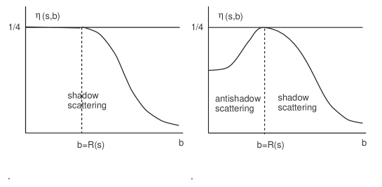
Figure 1: Impact parameter dependence of the inelastic overlap function in the standard unitarization scheme (left panel) and in the unitarization scheme with antishadowing (right panel).

The region of the LHC energies is the one where antishadow scattering mode is to be presented. It will be demonstrated in the next section that this mode can be revealed directly measuring $\sigma_{el}(s)$ and $\sigma_{tot}(s)$ and not only through the analysis in impact parameter representation.

3 Approach to asymptotics in the $U$–matrix model

To get the numerical estimates we shall use the following ansatz for the generalized reaction matrix

$$U(s,b)=ig\left[1+\alpha\frac{\sqrt{s}}{m_{Q}}\right]^{N}\exp(-Mb/\xi)\equiv ig(s)\exp(-Mb/\xi),$$ (13)

where $M=\sum^{N}_{q=1}m_{Q}$. Here $m_{Q}$ is the mass of constituent quark, which is taken to be $0.35$ $GeV$, $N$ is the total number of valence quarks in the colliding hadrons, i.e. $N=6$ for $pp$–scattering. The value for the other parameters were obtained in [19] and have the following values $g=0.24$, $\xi=2.5$, $\alpha=0.56\cdot 10^{-4}$. With these values of parameters the model provides satisfactory description of the available experimental data for the forward elastic $pp$-scattering. To obtain the above explicit form for the function $U(s,b)$ we used chiral quark model for $U$–matrix [21] where $U(s,b)$ is chosen as a product of the averaged quark amplitudes

$$U(s,b)=\prod^{N}_{Q=1}\langle f_{Q}(s,b)\rangle$$ (14)

in accordance with the assumed quasi-independence of valence quark scattering. The $b$–dependence of the function $\langle f_{Q}\rangle$ has a simple form $\langle f_{Q}\rangle\propto\exp(-m_{Q}b/\xi)$ which correspond to quark interaction radius $r_{Q}=\xi/m_{Q}$.

For the LHC energy $\sqrt{s}=14$ $TeV$ we have

$$\sigma_{tot}\simeq 230\;\mbox{mb}$$ (15)

and

$$\sigma_{el}/\sigma_{tot}\simeq 0.67.$$ (16)

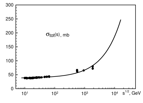
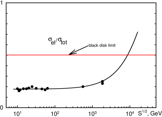
Figure 2: Total and ratio of elastic to total cross-sections of $pp$–interactions

Thus, the antishadow scattering mode could be discovered at LHC by measuring $\sigma_{el}/\sigma_{tot}$ ratio which is greater than the black disc value $1/2$ (cf. Fig. 2).

However, the LHC energy is not in the asymptotic region yet; the total, elastic and inelastic cross-sections behave like

$$\sigma_{tot,el}\propto\ln^{2}\left[g\left(1+\alpha\frac{\sqrt{s}}{m_{Q}}\right)^{N}\right],\;\sigma_{inel}\propto\ln\left[g\left(1+\alpha\frac{\sqrt{s}}{m_{Q}}\right)^{N}\right].$$ (17)

Asymptotical behavior

$$\sigma_{tot,el}\propto\ln^{2}s,\;\;\sigma_{inel}\propto\ln s$$ (18)

is expected at $\sqrt{s}>100$ $TeV$.

Another predictions of the chiral quark model is decreasing energy dependence of the the cross-section of the inelastic diffraction at $s>s_{0}$. Decrease of diffractive production cross–section at high energies ($s>s_{0}$) is due to the fact that $\eta(s,b)$ becomes peripheral at $s>s_{0}$ and the whole picture corresponds to the antishadow scattering at $b<R(s)$ and to the shadow scattering at $b>R(s)$ where $R(s)$ is the interaction radius:

$$\frac{d\sigma_{diff}}{dM_{X}^{2}}\simeq\frac{8\pi g^{*}\xi^{2}}{M_{X}^{2}}\eta(s,0).$$ (19)

The parameter $g^{*}<1$ is the probability of the excitation of a constituent quark during interaction. Diffractive production cross–section has the familiar $1/M^{2}$ dependence which is related in this model to the geometrical size of excited constituent quark.

At the LHC energy $\sqrt{s}=14$ $GeV$ the single diffractive inelastic cross-sections is limited by the value $\sigma_{diff}(s)\leq 2.4\;\mbox{mb}$.

The above predicted values for the global characteristics of $pp$ – interactions at LHC differ from the most common predictions of the other models. First, the total cross–section is predicted to be twice as much of the common predictions in the range 95-120 mb [22] and it even overshoots the existing cosmic ray data. However, extracting total proton–proton cross sections from cosmic ray experiments is model dependent and far from straightforward (see, e.g. [23] and references therein). Those experiments measure the attenuation lengths of the showers initiated by the cosmic particles in the atmosphere and are sensitive to the model dependent parameter called inelasticity. They do not provide any information on elastic scattering channel.

4 Angular structure of elastic scattering and diffraction dissociation

Elastic scattering amplitude $F(s,t)$ is determined by the singularities in the impact parameter complex plane $\beta=b^{2}$ plane. It has poles which positions are determined by the solutions of the following equation:

$$1+U(s,\beta)=0$$ (20)

and the branching point at $\beta=0$ (cf. Fig. 3), i.e.

$$F(s,t)=F_{p}(s,t)+F_{c}(s,t).$$

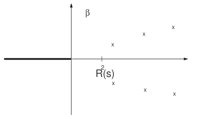
Figure 3: Singularities of scattering amplitude in the complex $\beta$-plane

Contribution of the poles located at the points

$$\beta_{n}(s)=\left[R(s)+i\frac{\xi}{M}\pi n\right]^{2},\quad n=\pm 1,\pm 3,...$$

where

$$R(s)=\frac{\xi}{M}\ln g(s)$$

determines the elastic amplitude in the region $|t|/s\ll 1\,(t\neq 0)$. The amplitude in this region can be represented in a form of series over the parameter $\tau(\sqrt{-t})$:

$$F(s,t)=s\sum_{k=1}^{\infty}\tau^{k}(\sqrt{-t})\varphi_{k}[R(s),\sqrt{-t}],$$ (21)

where the parameter $\tau$ decreases exponentially with $\sqrt{-t}$:

$$\tau(\sqrt{-t})=\exp(-\frac{2\pi\xi}{M}\sqrt{-t}).$$

This series provides diffraction peak and dip-bump structure of the differential cross-section in elastic scattering. In the region of moderate $t$ it is sufficient to keep few or even one of the terms of series Eq. (21). The differential cross-section in this region has well known Orear behavior. For elastic scattering amplitude $F(s,t)$ the pole and cut contributions are decoupled dynamically when $g(s)\rightarrow\infty$ at $s\rightarrow\infty$. At large momentum transfer ($s\to\infty$, $|t|/s$ - fixed) the contribution from the branching point ($\beta=0$) is a dominating one. The angular distribution in this region has the power dependence

$$\frac{d\sigma}{dt}\propto\left(\frac{1}{s}\right)^{N+3}f(\theta).$$ (22)

There is a direct interrelation of the power law behavior of the differential cross sections of large angle scattering with rising behavior of the total cross sections at high energies.

Similarity between elastic and inelastic diffraction in the $t$-channel approach suggests that the latter one would have similar to elastic scattering behavior of the differential cross-section. However, it cannot be taken for granted and e.g. transverse momentum distribution of diffractive events in the deep-inelastic scattering at HERA shows a power-like behavior without apparent dips [24]. Similar behavior was observed also in the hadronic diffraction dissociation process at CERN [1] where also no dip and bump structure was observed. Angular dependence of diffraction dissociation together with the measurements of the differential cross–section in elastic scattering would allow to determine the geometrical properties of elastic and inelastic diffraction, their similar and distinctive features and origin. In the $U$-matrix approach the impact parameter amplitude of diffraction dissociation $F_{diff}(s,b,M_{X})$ can be written in the pure imaginary case as a square root of the cross-section, i.e.

$$F_{diff}(s,b,M_{X})={\sqrt{U_{diff}(s,b,M_{X})}}/{[1+U(s,b)]}$$ (23)

and the amplitude $F_{diff}(s,t,M_{X})$ is

$$F_{diff}(s,t,M_{X})=\frac{is}{\pi^{2}}\int_{0}^{\infty}bdbJ_{0}(b\sqrt{-t}){\sqrt{U_{diff}(s,b,M_{X})}}/{[1+U(s,b)]}.$$ (24)

The corresponding amplitude $F_{diff}(s,t,M_{X})$ can be calculated analytically. To do so we continue the amplitudes $F_{diff}(s,\beta,M_{X}),\,\beta=b^{2}$, to the complex $\beta$–plane and then $F_{diff}(s,t,M_{X})$ can be represented as a sum of the pole contribution and the contribution of the cut [25]:

$$F_{diff}(s,t,M_{X})=F_{diff,p}(s,t,M_{X})+F_{diff,c}(s,t,M_{X})$$ (25)

The situation is different in the case of diffraction production. Instead of dynamical separation of the pole and cut contribution discussed above we have a suppression of the pole contribution at high energies since at fixed $t$

$$F_{diff,p}=O(s[g(s)]^{-\frac{M_{X}}{2{M}}}\ln^{1/2}g(s)),\quad F_{diff,c}=O(s[g(s)]^{-\frac{1}{2}}).$$ (26)

Therefore, at all $t$ values we will have

$$F_{diff}(s,t,M_{X})\simeq F_{diff,c}(s,t,M_{X}),$$ (27)

where

$$F_{diff,c}(s,t,M_{X})\simeq ig^{*}g^{-1/2}(s)(1-\frac{t}{\bar{M}_{X}^{2}})^{-3/2},$$ (28)

where $\bar{M}_{X}=(M_{X}-M-1)/2\xi$. This means that the differential cross-section of the diffraction production will have smooth dependence on $t$ with no apparent dips and bumps

$$\frac{d\sigma_{diff}}{dtdM_{X}^{2}}\propto(1-\frac{t}{\bar{M}_{X}^{2}})^{-3}.$$ (29)

It is interesting to note that at large values of $M_{X}\gg M$ the normalized differential cross-section $\frac{1}{\sigma_{0}}\frac{d\sigma}{dtdM_{X}^{2}}$ ($\sigma_{0}$ is the value of cross-section at $t=0$) will exhibit scaling behavior

$$\frac{1}{\sigma_{0}}\frac{d\sigma}{dtdM_{X}^{2}}=f(-t/M_{X}^{2}),$$ (30)

and explicit form of the function $f(-t/M_{X}^{2})$ is the following

$$f(-t/M_{X}^{2})=(1-4\xi^{2}t/M_{X}^{2})^{-3}.$$ (31)

This dependence is depicted on Fig. 4.

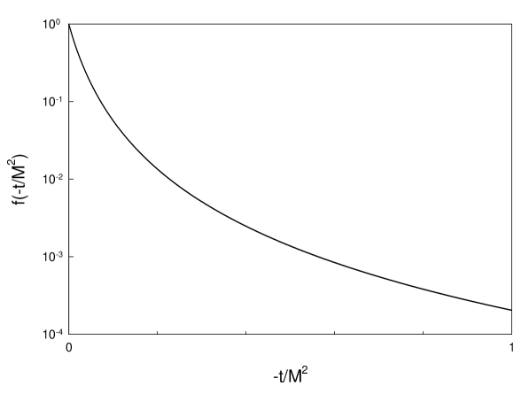
Figure 4: Scaling behavior of the normalized differential cross-section $\frac{1}{\sigma_{0}}\frac{d\sigma}{dtdM^{2}}$.

The above scaling has been obtained in the model approach, however it might have a more general meaning.

The angular structure of diffraction dissociation processes given by Eq. (29) takes place at high energies where $g(s)>1$ while at moderate and low energies where $g(s)\leq 1$ the both contributions from poles and cut are significant. In this region

$$F_{diff}(s,t,M_{X}^{2})=s\sum_{k=1}^{\infty}\tau^{k}(\sqrt{-t})\varphi_{diff,k}[R(s),\sqrt{-t},M_{X}^{2}],$$ (32)

where the parameter $\tau(\sqrt{-t})$ is the same as it is in the elastic scattering. Thus at low energies the situation is similar to the elastic scattering, i.e. diffraction cone and possible dip-bump structure should be present in the region of small values of $t$, and the overall behaviour of the differential cross-section will be rather complicated and incorporates diffraction cone, Orear type and power-like dependencies.

However, at high energies a simple power-like dependence on $t$ Eq. (29) is predicted. It was shown that the normalized differential cross-section has a scaling form and only depends on the ratio $-t/M_{X}^{2}$ at large values of $M_{X}^{2}$.

In fact, our particular comparative analysis of the poles and cut contributions has very little with the model form of the $U$–matrix. This is why it has a more general meaning.

At the LHC energies the diffractive events with the masses as large as 3 TeV could be studied. It would be interesting to check this prediction at the LHC where the scaling and simple power-like behavior of diffraction dissociation differential cross-section should be observed. Observation of such behavior would confirm the diffraction mechanism based on excitation of the complex hadronlike object – the constituent quark.

5 Angular distributions of leading protons in central production processes

It was proposed in [26] to study influence of centrally produced particles on the angular distribution of leading protons in the processes with two rapidity gaps, which are also known as a double Pomeron exchange (dpe) processes:

$$p+p\to p+X+p.$$ (33)

In what follows we will consider symmetrical case $t_{1}=t_{2}=t$. It is interesting to study how the diffractive pattern observed in elastic scattering will be changed in the corresponding processes with centrally produced particles.

First of all elastic scattering and process (33) are very different from the point of view of unitarity equation (1). The process (33) is one of the many contributing processes to the function $\eta(s,b)$ and consequently into the amplitude of elastic scattering $f(s,b)$. In the $U$-matrix approach the impact parameter amplitude of the process (33) $F_{dpe}(s,b,\zeta)$ can be written in the pure imaginary case according to (10) as a square root of the cross-section, i.e.

$$F_{dpe}(s,b,\zeta)={\sqrt{I(s,b,\zeta)}}/{[1+U(s,b)]}$$ (34)

and the amplitude $F_{dpe}(s,t,\zeta)$ is

$$F_{dpe}(s,t,\zeta)=\frac{is}{\pi^{2}}\int_{0}^{\infty}bdbJ_{0}(b\sqrt{-t}){\sqrt{I(s,b,\zeta)}}/{[1+U(s,b)]}.$$ (35)

The variable $t$ is the momentum transfer to one of the protons, while the variable $\zeta$ is related to the system of particles $X$ or to one particle from this system. Using relation (12) we can represent $I(s,b,\zeta)$ in the form

$$I(s,b,\zeta)=\Phi(s,b,\zeta)\mbox{Im}U(s,b),$$ (36)

where

$$\int\Phi(s,b,\zeta)d\zeta=\bar{n}(s,b).$$ (37)

For the mean multiplicity we suppose that the multiplicity of the centrally produced particles is given by the following expression

$$\bar{n}(s,b)=\beta N_{0}(s)D_{C}(b),$$ (38)

where the function $D_{C}(b)$ describes distribution of two hadron condensates clouds in the overlapping region. Arguments in favor of such form and assumed hadron structure are desribed in the next section. The corresponding amplitude $F_{dpe}(s,t,\zeta)$ can be calculated analytically and calculations are similar to the case of elastic scattering amplitude and amplitude of diffraction dissociation. It is necessary to continue the amplitudes $F_{dpe}(s,\beta,\zeta)$ ($\beta=b^{2}$), to the complex $\beta$–plane and transform the Fourier–Bessel integral over
impact parameter into the integral in the complex $\beta$ – plane over the contour $C$ which goes around the positive semiaxis. The amplitude $F_{dpe}(s,\beta,\zeta)$ has the poles and a branching point at $\beta=0$. Therefore it can be represented as a sum of the pole contributions and the contribution of the cut:

$$F_{dpe}(s,t,\zeta)=F_{dpe,p}(s,t,\zeta)+F_{dpe,c}(s,t,\zeta)$$ (39)

Then, using relation (37) and assuming

$$\Phi(s,b,\zeta)=\bar{n}(s,b)\phi(\zeta)$$

we obtain that

$$F_{dpe,p}\sim s\sum_{n=\pm 1,\pm 3,...}[\bar{n}(s,\sqrt{\beta_{n}})\phi(\zeta)]\sqrt{\beta_{n}}K_{0}(\sqrt{t\beta_{n}}),$$ (40)

i.e. diffractive pattern of leading protons will depend on the distribution of mean multiplicity in impact parameter of the centrally produced particles. Using for the mean multiplicity results described in Section 6, the amplitude (40) can be rewritten in the form

$$F_{dpe,p}\sim ss^{\frac{1}{4}(1-\frac{M_{C}\xi}{m_{Q}})}\phi(\zeta)\sum_{n=\pm 1,\pm 3,...}e^{i\pi n\frac{M_{C}\xi}{2M}}\sqrt{\beta_{n}}K_{0}(\sqrt{t\beta_{n}})$$ (41)

Thus, the presence of oscillating factor $e^{i\pi n\frac{M_{C}\xi}{2M}}$ would lead to significant differences in the diffractive patterns of leading protons in the processes (33) and elastic scattering. Indeed, at small values of $t$ all terms of the series (41) are important. In elastic scattering the summation over all $n$ leads to the exponential behavior of the differential cross section [21]:

$$\frac{d\sigma}{dt}\propto\exp\left(B(s)t\right),\quad B(s)\propto\ln^{2}s.$$ (42)

However, for the process (33) the terms with the large values of $n$ will be suppressed due the oscillation factor. Thus, we expect that the Orear type behaviour will lake place already at low values of $t$ and differential cross section would have the following $t$–dependence already at small and moderate values of $t$:

$$\frac{d\sigma}{dtd\zeta}\propto\exp\left(-\frac{2\pi\xi}{M}\sqrt{-t}\right).$$ (43)

6 Multiparticle production and antishadowing

The region of the LHC energies is the one where new, antishadow scattering mode can be observed. Immediate question arises on consistency of the antishadowing with the growth of mean multiplicity in hadronic collisions with energy. Moreover, many models and the experimental data suggest a power-like energy dependence of mean multiplicity and a priori the compatibility of such dependence with antishadowing is not evident.

Now we turn to the mean multiplicity and consider first the corresponding quantity in the impact parameter representation. As it follows from (11) and (12) the $n$–particle production cross–section $\sigma_{n}(s,b)$

$$\sigma_{n}(s,b)=\frac{\bar{U}_{n}(s,b)}{|1-iU(s,b)|^{2}}$$ (44)

Then the probability

$$P_{n}(s,b)\equiv\frac{\sigma_{n}(s,b)}{\sigma_{inel}(s,b)}=\frac{\bar{U}_{n}(s,b)}{\mbox{Im}U(s,b)}.$$ (45)

Thus, we observe the cancellation of unitarity corrections in the ratio of the cross-sections $\sigma_{n}(s,b)$ and $\sigma_{inel}(s,b)$. Therefore the mean multiplicity in the impact parameter representation

$$\bar{n}(s,b)=\sum_{n}nP_{n}(s,b)$$

is not affected by unitarity corrections and therefore cannot be proportional to $\eta(s,b)$. This conclusion is consistent with Eq. (12). The above mentioned proportionality is a rather natural assumption in the framework of the geometrical models, but it is in conflict with the unitarity. Because of that the results [30] based on such assumption should be taken with precaution. However, the above cancellation of unitarity corrections does not take place for the quantity $\bar{n}(s)$ which we address now.

We use a model for the hadron scattering described in [21] which is based on the ideas of chiral quark models. The picture of a hadron consisting of constituent quarks embedded into quark condensate implies that overlapping and interaction of peripheral clouds occur at the first stage of hadron interaction (Fig. 5). Nonlinear field couplings could transform then the kinetic energy to the internal energy and mechanism of such transformation was discussed by Heisenberg [10] and Carruthers [31]. As a result massive virtual quarks appear in the overlapping region and some effective field is generated. Valence constituent quarks located in the central part of hadrons are supposed to scatter simultaneously in a quasi-independent way by this effective field.

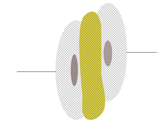
Figure 5: Schematic view of initial stage of the hadron interaction.

Massive virtual quarks play a role of scatterers for the valence quarks in elastic scattering and their hadronization leads to production of secondary particles in the central region. To estimate number of such scatterers one could assume that part of hadron energy carried by the outer condensate clouds is being released in the overlap region to generate massive quarks. Then this number can be estimated by:

$$\tilde{N}(s,b)\,\propto\,\frac{(1-\langle k_{Q}\rangle)\sqrt{s}}{m_{Q}}\;D^{h_{1}}_{c}\otimes D^{h_{2}}_{c}\equiv N_{0}(s)D_{C}(b),$$ (46)

where $m_{Q}$ – constituent quark mass, $\langle k_{Q}\rangle$ – average fraction of hadron energy carried by the constituent valence quarks. Function $D^{h}_{c}$ describes condensate distribution inside the hadron $h$, and $b$ is an impact parameter of the colliding hadrons.

Thus, $\tilde{N}(s,b)$ quarks appear in addition to $N=n_{h_{1}}+n_{h_{2}}$ valence quarks. In elastic scattering those quarks are transient ones: they are transformed back into the condensates of the final hadrons. Calculation of elastic scattering amplitude has been performed in [21]. However, valence quarks can excite a part of the cloud of the virtual massive quarks and these virtual massive quarks will subsequently fragment into the multiparticle final states. Such mechanism is responsible for the particle production in the fragmentation region and should lead to strong correlations between secondary particles. It means that correlations exist between particles from the same (short–range correlations) and different clusters (long–range correlations) and, in particular, the forward–backward multiplicity correlations should be observed. This mechanism can be called as a correlated cluster production mechanism. Evidently, similar mechanism should be significantly reduced in $e^{+}e^{-}$–annihilation processes and therefore large correlations are not to be expected there.

As it was already mentioned simple (not induced by interactions with valence quarks) hadronization of massive $\tilde{N}(s,b)$ quarks leads to formation of the multiparticle final states, i.e. production of the secondary particles in the central region. The latter should not provide any correlations in the multiplicity distribution.

Remarkably, existence of the massive quark-antiquark matter in the stage preceding hadronization seems to be supported by the experimental data obtained at CERN SPS and RHIC (see [32] and references therein).

Since the quarks are constituent, it is natural to expect direct proportionality between a secondary particles multiplicity and number of virtual massive quarks appeared (due to both mechanisms of multiparticle production) in collision of the hadrons with given impact parameter:

$$\bar{n}(s,b)=\alpha(n_{h_{1}}+n_{h_{2}})N_{0}(s)D_{F}(b)+\beta N_{0}(s)D_{C}(b),$$ (47)

with constant factors $\alpha$ and $\beta$ and

$$D_{F}(b)\equiv D_{Q}\otimes D_{C},$$

where the function $D_{Q}(b)$ is the probability amplitude of the interaction of valence quark with the excitation of the effective field, which is in fact related to the quark matter distribution in this hadron-like object called the valence constituent quark [21]. The mean multiplicity $\bar{n}(s)$ can be calculated according to the formula

$$\bar{n}(s)=\frac{\int_{0}^{\infty}\bar{n}(s,b)\eta(s,b)bdb}{\int_{0}^{\infty}\eta(s,b)bdb}.$$ (48)

It is evident from Eq. (48) and Fig. 1 that the antishadow mode with the peripheral profile of $\eta(s,b)$ suppresses the region of small impact parameters, and the main contribution to the mean multiplicity is due to peripheral region of $b\sim R(s)$.

To make explicit calculations we model for simplicity the condensate distribution $D_{C}(b)$ and the impact parameter dependence of the probability amplitude $D_{Q}(b)$ of the interaction of valence quark with the excitation of the effective field by the exponential forms, and thus we use exponential dependencies for the functions $D_{F}(b)$ and $D_{C}(b)$ with the different radii. Then the mean multiplicity

$$\bar{n}(s,b)=\tilde{\alpha}N_{0}(s)\exp(-b/R_{F})+\tilde{\beta}N_{0}(s)\exp(-b/R_{C}).$$ (49)

After calculation of the integrals (48) we arrive to the power-like dependence of the mean multiplicity $\bar{n}(s)$ at high energies

$$\bar{n}(s)=as^{\delta_{F}}+bs^{\delta_{C}},$$ (50)

where

$$\delta_{F}={\frac{1}{2}\left(1-\frac{\xi}{m_{Q}R_{F}}\right)}\quad\mbox{and}\quad\delta_{C}={\frac{1}{2}\left(1-\frac{\xi}{m_{Q}R_{C}}\right)}.$$

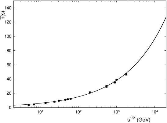
Figure 6: Energy dependence of mean multiplicity, theoretical curve is given by the equation $\bar{n}(s)=as^{\delta}$ ($a=2.328$, $\delta=0.201$); experimental data from the Refs. [33].

There are four free parameters in the model, $\tilde{\alpha}$, $\tilde{\beta}$ and $R_{F}$, $R_{C}$, and the freedom in their choice is translated to $a$, $b$ and $\delta_{F}$, $\delta_{C}$. The value of $\xi=2$ is fixed from the data on angular distributions [21] and for the mass of constituent quark the standard value $m_{Q}=0.35$ GeV was taken. However, fit to experimental data on the mean multiplicity leads to approximate equality $\delta_{F}\simeq\delta_{C}$ and actually Eq. (50) is reduced to the two-parametric power-like energy dependence of mean multiplicity

$$\bar{n}=as^{\delta},$$

which is in good agreement with the experimental data (Fig. 6). Equality $\delta_{F}\simeq\delta_{C}$ means that variation of the correlation strength with energy is weaker than the power-like one and could be described, e.g. by a logarithmic function of energy. From the comparison with the data on mean multiplicity we obtain that $\delta\simeq 0.2$, which corresponds to the effective masses, which are determined by the respective radii ($M=1/R$), $M_{C}\simeq M_{F}\simeq 0.3m_{Q}$, i.e. $M_{F}\simeq M_{C}\simeq m_{\pi}$.

The value of mean multiplicity expected at the LHC energy ($\sqrt{s}=14$ TeV) is about 110. It is not surprising that it is impossible to differentiate contributions from the two mechanisms of particle production at the level of mean multiplicity. The studies of correlations are necessary for that purpose.

Multiplicity distribution $P_{n}(s,b)$ and mean multiplicity $\bar{n}(s,b)$ in the impact parameter representation have no absorptive corrections, but since antishadowing leads to suppression of particle production at small impact parameters and the main contribution to the integral multiplicity $\bar{n}(s)$ comes from the region of $b\sim R(s)$. Of course, this prediction is to be valid for the energy range where antishadow scattering mode starts to develop and is therefore consistent with the “centrality” dependence of the mean multiplicity observed at RHIC [35].

It would be interesting to note that due to peripheral form of the inelastic overlap function the secondary particles will be mainly produced at impact parameters $b\sim R(s)$ and thus will carry out large orbital angular momentum

$$L\simeq R(s)\frac{\sqrt{s}}{2}\bar{n}(s,b=R(s)).$$

To compensate this orbital momentum spins of secondary particles should become lined up, i.e. the spins of the produced particles should demonstrate significant correlations when the antishadow scattering mode appears. Similar conclusion on spin correlations of secondary particles has been made long time ago by Yang and Chou under utilization of the concept of partition temperature in the geometric model for hadron production [36].

It is also worth noting that no limitations follow from the general principles for the mean multiplicity, besides the well known one based on the energy conservation law. Having in mind relation (49), we could say that the obtained power–like dependence which takes into account unitarity effects could be considered as a kind of a saturated upper bound for the mean multiplicity growth.

Elastic scattering domination at the LHC and the appearance of the antishadow scattering mode implies a somewhat unusual scattering picture. At high energies the proton should be represented as a very loosely bounded composite system and it appears that this system has a high probability to reinstate itself only in the central collisions where all of its parts participate in the coherent interactions. Therefore the central collisions are responsible for elastic processes while the peripheral ones where only few parts of weekly bounded protons are involved result in the production of the secondary particles. This leads to the peripheral impact parameter profile of the inelastic overlap function. Such evolution could be accomplished with spin correlations of the produced particles.

7 Polarization measurements

In soft hadronic interactions significant single-spin effects could be expected since the helicity conservation does not work for interactions at large distances, once the chiral $SU(3)_{L}\times SU(3)_{R}$ symmetry of the QCD Lagrangian is spontaneously broken in the real world. Thus, studies of the $p_{\perp}$–dependence of the one–spin asymmetries can be used as a way to reveal a transition from a non–perturbative phase ($P\neq 0$) to the perturbative one ($P=0$). The essential point here is an assumption that at short distances the vacuum is perturbative. However, the very existence of the above transition can not be taken for granted since the vacuum, even at short distances, could be filled up with the fluctuations of gluon and quark fields. The measurements of the one–spin transverse asymmetries and polarization is an important probe of the chiral structure of the effective QCD Lagrangian.

At the same time we can note that polarization effects as well as some other recent experimental data demonstrate that hadron interactions have a significant degree of coherence. Experimentally, spin asymmetries increase at high transverse momentum in elastic scattering and are flat in inclusive processes.

It is interesting to note that on the base of the model in [37] one should expect a zero polarization in the region where quark–gluon plasma (QGP) has been formed, since chiral symmetry is restored and there is no room for quasiparticles such as constituent quarks. Thus, the absence or strong diminishing e. g. of transverse hyperon polarization can be used as a signal of QGP formation in heavy-ion collisions. This prediction should also be valid for the models based on confinement, e.g. the Lund and Thomas precession model. We could use a vanishing polarization of e. g. $\Lambda$–hyperons in heavy ion collisions as a sole result of QGP formation provided the corresponding observable is non-zero in proton–proton collisions. The prediction based on this observation would be a decreasing behavior of polarization of $\Lambda$ with the impact parameter in heavy-ion collisions in the region of energies and densities where QGP was produced:

$$P_{\Lambda}(b)\to 0\quad\mbox{at}\quad b\to 0,$$ (51)

since the overlap is maximal at $b=0$. The value of the impact parameter can be controlled by the centrality in heavy–ion collisions. The experimental program could therefore include measurements of $\Lambda$–polarization in $pp$–interactions first, and then if a significant polarization would be measured, the corresponding measurements could be a useful tool for the QGP detection. Such measurements seem to be experimentally feasible at RHIC and LHC provided it is supplemented with forward detectors.

Conclusion

The possibility to reveal a new scattering mode at the LHC is an intriguing one. It would significantly change our picture of hadron scattering and lead to better understanding of the non-perturbative region of QCD. Diffraction and related processes are very important for studies of collective, coherent phenomena in hadronic interactions. Predictions for the experimental observables in these processes presented in this review and their experimental verifications will certainly increase the scope of strong interaction studies at the LHC.

References

- [1] R. Bonino et al.//Phys. Lett. B 1988. V.211. P.239. ; A. Brandt et al., Nucl. Phys.// B 1998. V.514. P.3.
- [2] T. Ahmed et al.// Phys. Lett. B 1995. V.348. P.681.
- [3] M. Derrick et al.// Z. Phys. C 1995. V.68. P.569.
- [4] C. Adloff et al.// Z. Phys. C 1997. V.76. P.613.
- [5] L. Alvero et al.//Phys. Rev. D 1999. V.59. P.074022.
- [6] J. D. Bjorken// Invited talk at 7th Conference on Intersections Between Particle and Nuclear Physics (CIPANP 2000), Quebec City, Quebec, Canada, 22-28 May 2000. Published in AIP Conf.Proc. 2002. V.549. P.211.; hep-ph/0008048.
- [7] A. Ageev et al.// J. Phys. G 2002. V.28. P.R117.
- [8] A. A. Logunov, Nguyen Van Hieu, O. A. Khrustalev, Essays dedicated to Nikolai N. Bogolyubov on the occasion of his sixtieth birthday, Moscow, Nauka, 1969. P.90.
- [9] S. M. Troshin and N. E. Tyurin// Eur. Phys. J. C 2001. V.21. P.679.; V.A. Petrov, A. V. Prokudin, S. M. Troshin and N. E. Tyurin// J. Phys. G 2001. V.27. P.2225.
- [10] W. Heisenberg// Z. Phys. 1952. V.133. P.65.
- [11] S. M. Troshin and N. E. Tyurin// Phys. Lett. B 1993. V.316. P.175.
- [12] S. M. Troshin and N. E. Tyurin// Phys. Part. Nucl. 1999. V.30. P.550.
- [13] A. A. Logunov, V.I. Savrin, N. E. Tyurin and O. A. Khrustalev// Teor. Mat. Fiz. 1971. V.6. P.157.
- [14] C. T. Sachrajda and R. Blankenbecler// Phys. Rev. D 1975. V.12. P.1754.
- [15] R. Blankenbecler and M. L. Goldberger// Phys. Rev. 1962. V.126. P.766.
- [16] M. Baker and R. Blankenbecler// Phys. Rev. 1962. V.128. P.415.
- [17] S. M. Troshin and N. E. Tyurin// Teor. Mat. Fiz. 1976. V.28. P.139.
- [18] S. M. Troshin and N. E. Tyurin// Z. Phys. C 1989. V.45. P.171.
- [19] P.M. Nadolsky, S. M. Troshin and N. E. Tyurin// Z. Phys. C 1995. V.69. P.131.
- [20] P.Desgrolard , L. Jenkovszky, B. Struminsky// Eur. Phys. J. C 1999. V.11. P.144.
- [21] S.M. Troshin and N.E. Tyurin// Nuovo Cim. A 1993. V.106. P.327.; Proc. of the Vth Blois Workshop on Elastic and Diffractive Scattering, Providence, Rhode Island, P.387 1993; Phys. Rev. D 1994. V.49. P.4427.; Z. Phys. C 1994. V.64. P.311.
- [22] J. Velasco , J. Perez-Peraza, A. Gallegos-Cruz, M. Alvarez-Madrigal, A. Faus-Golfe, A. Sanchez-Hertz// hep-ph/9910484
- [23] M. M. Block, F. Halzen and T. Stanev// hep-ph/9908222.
- [24] C. Adloff et al.// Eur. Phys. J. C 1998. V.10. P.443.
- [25] S. M. Troshin and N. E. Tyurin// hep-ph/0008274.
- [26] V.A. Petrov// talk given at the International Symposium “ LHC Physics and Detectors”, Dubna, 28-30 June 2000.
- [27] J. Manjavidze and A. Sissakian// Phys. Rept. 2001. V.346. P.1.
- [28] P.C. Beggio, M.J. Menon and P.Valin// Phys. Rev. D 2000. V.61. P.034015.
- [29] F. Ravndal// ”Feynman’s (secret?) parton model for diffraction scattering”, contributed paper presented at the Conference QCD — 20 Years Later, Aachen, June 9-13, 1992; further discussions of this paper and model can be found in S. Barshay, P.Heiliger and D. Rein, Mod. Phys. Lett A 1992. V.7. P.2559.
- [30] L. L. Jenkovszky and B.V.Struminsky// hep-ph/0205322.
- [31] P.Carruthers// Nucl. Phys. A 1984. V.418. P.501.
- [32] J. Zimányi, P.Lévai, T.S. Biró// hep-ph/0205192.
-
[33]
G.J. Alner et al.// Phys. Lett. B 1985. V.160. P.199.;
C. Albajar et al.// Nucl. Phys. B 1988. V.309. P.405.;
R. E. Ansorge et al.// Z. Phys. C 1987. V.43. P.357.;
G. J. Alner et al.// Phys. Rep. 1987. V.154 P.247.;
T. Alexopoulos et al.// Phys. Lett. B 1998. V.435. P.453. - [34] S. Barshay and G. Kreyerhoff// Nucl. Phys. A 2002. V.697. P.563.
- [35] K. Adcox et al. (PHENIX Collaboration)// Phys. Rev. Lett. 2001. V.86. P.3500.
- [36] C. N. Yang and T. T. Chou// J. Phys. Soc. Japan 1986. V.55. P.53.
- [37] S. M. Troshin and N. E. Tyurin// Phys. Rev. D 1997. V.55. P.1265.