Impact of $U_{e3}$ on Neutrino Models

Morimitsu Tanimoto

Department of Physics, Niigata University, Ikarashi 2-8050, 950-2181 Niigata, JAPAN

ABSTRACT

We have discussed the impact of $U_{e3}$ on the model of the neutrino mass matrix. In order to get the small $U_{e3}$, some flavor symmetry is required. Typical two models are investigated. The first one is the model in which the bi-maximal mixing is realized at the symmetric limit. The second one is the texture zeros of the neutrino mass matrix.

1 Introduction

In these years empirical understanding of the mass and mixing of neutrinos have been advanced [1, 2, 3]. The KamLAND experiment selected the neutrino mixing solution that is responsible for the solar neutrino problem nearly uniquely [4], only large mixing angle solution. We have now good understanding concerning the neutrino mass difference squared and neutrino flavor mixings [5]. A constraint has also been placed on the mixing from the reactor experiment of CHOOZ [6].

These results indicate two large flavor mixings and one small flavor mixing. It is therefore important to investigate how the textures of lepton mass matrices can link up with the observables of the flavor mixing. There are some ideas to explain the large mixing angles. The mass matrices, which lead to the large mixing angle, are “lopsided mass matrix”[7], “democratic mass matrix” [8] and “Zee mass matrix”[9]. These textures are reconciled with some flavor symmetry.

We have another problem. Is the small $U_{e3}$ always guaranteed in the model with two large mixing angles? The answer is “No”. There are some models to give a large $U_{e3}$. The typical one is “Anarchy” mass matrix [10], which gives a rather large $U_{e3}$. Another example is the model, in which the large solar neutrino mixing comes from the charged lepton sector while the large atmospheric neutrino mixing comes from the neutrino sector. In this model $U_{e3}=1/2$ is predicted.

In order to get the small $U_{e3}$, some flavor symmetry is required. Typical two models are investigated in this talk. The first one is the model in which the bi-maximal mixing is realized at the symmetric limit. The second one is the texture zeros of the neutrino mass matrix.

2 Deviation from the Bi-Maximal Mixings

We consider the symmetric limit with the bi-maximal flavor mixing at which $U_{e3}=0$ as follows [11]:

$$\nu_{\alpha}=U^{(0)}_{\alpha i}\nu_{i}\ ,$$ (1)

where

$$U^{(0)}=\left(\matrix{\frac{1}{\sqrt{2}}&\frac{1}{\sqrt{2}}&0\cr-\frac{1}{2}&\frac{1}{2}&\frac{1}{\sqrt{2}}\cr\frac{1}{2}&-\frac{1}{2}&\frac{1}{\sqrt{2}}\cr}\right)\ .$$ (2)

One can parametrize the deviation $U^{(1)}$ in $\nu_{\alpha}=[U^{(1)^{\dagger}}U^{(0)}]_{\alpha i}\nu_{i}$ as follows:

$$U^{(1)}=\left(\matrix{c^{1}_{13}c^{1}_{12}&c^{1}_{13}s^{1}_{12}&s^{1}_{13}e^{-i\phi}\cr-c^{1}_{23}s^{1}_{12}-s^{1}_{23}s^{1}_{13}c^{1}_{12}e^{i\phi}&c^{1}_{23}c^{1}_{12}-s^{1}_{23}s^{1}_{13}s^{1}_{12}e^{i\phi}&s^{1}_{23}c^{1}_{13}\cr s^{1}_{23}s^{1}_{12}-c^{1}_{23}s^{1}_{13}c^{1}_{12}e^{i\phi}&-s^{1}_{23}c^{1}_{12}-c^{1}_{23}s^{1}_{13}s^{1}_{12}e^{i\phi}&c^{1}_{23}c^{1}_{13}\cr}\right)$$ (3)

where $s^{1}_{ij}\equiv\sin{\theta^{1}_{ij}}$ and $c^{1}_{ij}\equiv\cos{\theta^{1}_{ij}}$ denote the mixing angles in the bi-maximal basis and $\phi$ is the CP violating Dirac phase. The mixings $s^{1}_{ij}$ are expected to be small since these are deviations from the bi-maximal mixing. Here, the Majorana phases are absorbed in the neutrino mass eigenvalues.

Let us assume the mixings $s^{1}_{ij}$ to be hierarchical like the ones in the quark sector, $s^{1}_{12}\gg s^{1}_{23}\gg s^{1}_{13}$. Then, taking the leading contribution due to $s^{1}_{12}$, we have

$$|U_{e1}|\simeq\frac{1}{\sqrt{2}}\left(c^{1}_{12}+\frac{1}{\sqrt{2}}s^{1}_{12}\right)\ ,\quad|U_{e2}|\simeq\frac{1}{\sqrt{2}}\left(c^{1}_{12}-\frac{1}{\sqrt{2}}s^{1}_{12}\right)\ ,$$ (4)

which lead to

$$\tan^{2}\theta_{\rm sol}=\left(\frac{c^{1}_{12}-\frac{1}{\sqrt{2}}s^{1}_{12}}{c^{1}_{12}+\frac{1}{\sqrt{2}}s^{1}_{12}}\right)^{2}=1-2\sqrt{2}s^{1}_{12}+\mathrm{O}({(s^{1}_{12})}^{2})\,.$$ (5)

Thus, the solar neutrino mixing is somewhat reduced due to $s^{1}_{12}$. By using the data of the solar neutrino mixing, we predict the small $U_{e3}$ such as

$$|U_{e3}|\simeq\frac{1}{\sqrt{2}}s^{1}_{12}=0.03\sim 0.2\ ,$$ (6)

which is testable in the future experiments. In the next section, we present another approach, texture zeros.

3 Texture Zeros of Neutrino Mass Matrix

The texture zeros of the neutrino mass matrix have been discussed to explain these neutrino masses and mixings [12, 13, 14]. Recently, Frampton, Glashow and Marfatia [15] found acceptable textures of the neutrino mass matrix with two independent vanishing entries in the basis of the diagonal charged lepton mass matrix. The KamLAND result has stimulated the phenomenological analyses of the texture zeros [16, 17, 18, 19]. These results favour texture zeros for the neutrino mass matrix phenomenologically.

There are 15 textures with two zeros for the effective neutrino mass matrix $M_{\nu}$, which have five independent parameters. The two zero conditions give

$$(M_{\nu})_{ab}=\sum^{3}_{i=1}U_{ai}U_{bi}\lambda_{i}=0\ ,\qquad\qquad(M_{\nu})_{\alpha\beta}=\sum^{3}_{i=1}U_{\alpha i}U_{\beta i}\lambda_{i}=0\ ,$$ (7)

where $\lambda_{i}$ is the i-th eigenvalue including the Majorana phase, and indices $(ab)$ and $(\alpha\beta)$ denote the flavor components, respectively.

Solving these equations, the ratios of neutrino masses $m_{1}$, $m_{2}$, $m_{3}$, which are absolute values of $\lambda_{i}$’s, are given in terms of the neutrino mixing matrix $U$ [20] as follows:

$$\frac{m_{1}}{m_{3}} = \left|\frac{U_{a3}U_{b3}U_{\alpha 2}U_{\beta 2}-U_{a2}U_{b2}U_{\alpha 3}U_{\beta 3}}{U_{a2}U_{b2}U_{\alpha 1}U_{\beta 1}-U_{a1}U_{b1}U_{\alpha 2}U_{\beta 2}}\right|\ ,$$

$$\frac{m_{2}}{m_{3}} = \left|\frac{U_{a1}U_{b1}U_{\alpha 3}U_{\beta 3}-U_{a3}U_{b3}U_{\alpha 1}U_{\beta 1}}{U_{a2}U_{b2}U_{\alpha 1}U_{\beta 1}-U_{a1}U_{b1}U_{\alpha 2}U_{\beta 2}}\right|\ .$$ (8)

Then, one can test textures in the ratio $R_{\nu}$,

$$R_{\nu}\equiv\left|\frac{m^{2}_{2}-m^{2}_{1}}{m^{2}_{3}-m^{2}_{2}}\right|\approx\frac{\Delta m^{2}_{\rm sun}}{\Delta m^{2}_{\rm atm}}\ ,$$ (9)

which has been given by the experimental data. The ratio $R_{\nu}$ is given only in terms of four parameters (three mixing angles and one phase) in

$$U=\left(\matrix{c_{13}c_{12}&c_{13}s_{12}&s_{13}e^{-i\delta}\cr-c_{23}s_{12}-s_{23}s_{13}c_{12}e^{i\delta}&c_{23}c_{12}-s_{23}s_{13}s_{12}e^{i\delta}&s_{23}c_{13}\cr s_{23}s_{12}-c_{23}s_{13}c_{12}e^{i\delta}&-s_{23}c_{12}-c_{23}s_{13}s_{12}e^{i\delta}&c_{23}c_{13}\cr}\right)$$ (10)

where $c_{ij}$ and $s_{ij}$ denote $\cos\theta_{ij}$ and $\sin\theta_{ij}$, respectively.

Seven acceptable textures with two independent zeros were found for the neutrino mass matrix [15], and they have been studied in detail [17, 18]. Among them, the textures $\rm A_{1}$ and $\rm A_{2}$ [15], which correspond to the hierarchical neutrino mass spectrum, are strongly favoured by the recent phenomenological analyses [16, 17, 18]. Therefore, we study these two textures in this paper.

In the texture $A_{1}$, which has two zeros as $(M_{\nu})_{ee}=0$ and $(M_{\nu})_{e\mu}=0$, the mass ratios are given as

$$\frac{m_{1}}{m_{3}} = \left|\frac{s_{13}}{c^{2}_{13}}\left(\frac{s_{12}s_{23}}{c_{12}c_{23}}-s_{13}e^{-i\delta}\right)\right|\ ,$$

$$\frac{m_{2}}{m_{3}} = \left|\frac{s_{13}}{c^{2}_{13}}\left(\frac{c_{12}s_{23}}{s_{12}c_{23}}+s_{13}e^{-i\delta}\right)\right|\ .$$ (11)

In the texture $A_{2}$, which has two zeros as $(M_{\nu})_{ee}=0$ and $(M_{\nu})_{e\tau}=0$, the mass ratios are given as

$$\frac{m_{1}}{m_{3}} = \left|\frac{s_{13}}{c^{2}_{13}}\left(\frac{s_{12}c_{23}}{c_{12}s_{23}}+s_{13}e^{-i\delta}\right)\right|\ ,$$

$$\frac{m_{2}}{m_{3}} = \left|\frac{s_{13}}{c^{2}_{13}}\left(\frac{c_{12}c_{23}}{s_{12}s_{23}}-s_{13}e^{-i\delta}\right)\right|\ .$$ (12)

If $\theta_{12}$, $\theta_{23}$, $\theta_{13}$ and $\delta$ are fixed, we can predict $R_{\nu}$ in eq.(9), which can be compared with the experimental value ${\Delta m^{2}_{\rm sun}}/{\Delta m^{2}_{\rm atm}}$.

Taking account of the following data with $90\%$ C.L. [5],

$$\sin^{2}2\th_{\rm atm}\geq 0.92\ ,\qquad \Delta m^{2}_{\rm atm}=(1.5\sim 3.9)\times 10^{-3}{\rm eV}^{2}\ ,$$

$$\tan^{2}\th_{\rm sun}=0.33\sim 0.67\ ,\qquad \Delta m_{\rm sun}^{2}=(6\sim 8.5)\times 10^{-5}{\rm eV}^{2}\ ,$$ (13)

with $\sin\th_{\scriptscriptstyle\rm CHOOZ}\leq 0.2$, we predict $R_{\nu}$.

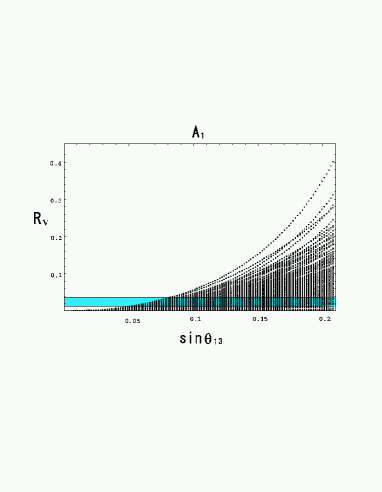
Figure 1: Scatter plot of $R_{\nu}$ versus $\sin\theta_{13}$ for the texture $A_{1}$. The unknown phase $\delta$ is taken in the whole region $-\pi\sim\pi$. The gray horizontal band is the experimental allowed region.

In Fig.1, we present the scatter plot of the predicted $R_{\nu}$ versus $\sin\theta_{13}$, in which $\delta$ is taken in the whole range $-\pi\sim\pi$ for the texture $A_{1}$. The parameters are taken in the following ranges in $\theta_{12}=30^{\circ}\sim 39^{\circ}$, $\theta_{23}=37^{\circ}\sim 53^{\circ}$, $\theta_{13}=1^{\circ}\sim 12^{\circ}$ and $\delta=-\pi\sim\pi$ with constant distributions those are flat on a linear scale. It is found that many predicted values of $R_{\nu}$ lie outside the experimental allowed region. This result means that some tunings among four parameters are demanded to be consistent with the experimental data. We get $\sin\theta_{13}\geq 0.05$ from the experimental value of $R_{\nu}$ as seen in Fig.1.

In order to present the allowed region of $\sin\theta_{13}$, we show the scatter plot of $\sin\theta_{13}$ versus $\tan^{2}\theta_{12}$ and $\tan^{2}\theta_{23}$ in Fig.2 and Fig.3, respectively, for the texture $A_{1}$. For the texture $A_{2}$, the numerical results is similar with the one in the texture $A_{1}$ because those are obtained only by replacing $\tan\theta_{23}$ in $A_{1}$ with $-\cot\theta_{23}$.

The allowed regions in Fig.2 and Fig.3 are quantitatively understandable in the following approximate relations:

$$|U_{e3}|\equiv\sin\theta_{13}\simeq\frac{1}{2}\tan 2\theta_{12}\ \cot\theta_{23}\sqrt{R_{\nu}\cos 2\theta_{12}}\ ,$$ (14)

for the texture $A_{1}$, and

$$|U_{e3}|\equiv\sin\theta_{13}\simeq\frac{1}{2}\tan 2\theta_{12}\ \tan\theta_{23}\sqrt{R_{\nu}\cos 2\theta_{12}}\ ,$$ (15)

for the texture $A_{2}$, respectively, where the phase $\delta$ is neglected because it is a next leading term. As $\tan\theta_{12}$ increases, the lower bound of $|U_{e3}|$ increases, and as $\tan\theta_{23}$ decreases, it increases. It is found in Fig.2 that the lower bound $|U_{e3}|=0.05$ is given in the case of the smallest $\tan^{2}\theta_{12}$, while $|U_{e3}|=0.08$ is given in the largest $\tan^{2}\theta_{12}$. On the other hand, as seen in Fig.3, the lower bound $|U_{e3}|=0.05$ is given in the largest $\tan^{2}\theta_{23}$, while $|U_{e3}|=0.08$ is given in the smallest $\tan^{2}\theta_{23}$. In the future, error bars of experimental data in eq.(13) will be reduced. Especially, KamLAND is expected to determine $\Delta m^{2}_{12}$ precisely. Therefore, the predicted region of $|U_{e3}|$ will be reduced significantly in the near future.

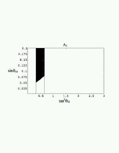
Figure 2: Scatter plot of $\sin\theta_{13}$ versus $\tan^{2}\theta_{12}$ for the texture $A_{1}$.

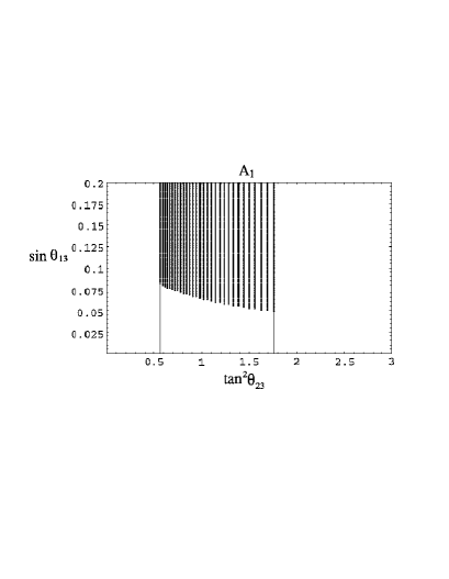
Figure 3: Scatter plot of $\sin\theta_{13}$ versus $\tan^{2}\theta_{23}$ for the texture $A_{1}$.

Above predictions are important ones in the texture zeros. The relative magnitude of each entry of the neutrino mass matrix is roughly given as follows:

$$M_{\nu}\sim\left(\matrix{{0}&{0}&\lambda\cr{0}&1&1\cr\lambda&1&1\cr}\right)\ \ \ {\rm for\ A_{1}}\ ,\qquad\qquad\left(\matrix{0&\lambda&0\cr\lambda&1&1\cr 0&1&1\cr}\right)\ \ \ {\rm for\ A_{2}}\ ,$$ (16)

where $\lambda\simeq 0.2$. However, these texture zeros are not preserved to all orders. Even if zero-entries of the mass matrix are given at the high energy scale, non-zero components may evolve instead of zeros at the low energy scale due to radiative corrections. Those magnitudes depend on unspecified interactions from which lepton masses are generated. Moreover, zeros of the neutrino mass matrix are given while the charged lepton mass matrix has off-diagonal components in the model with some flavor symmetry. Then, zeros are not realized in the diagonal basis of the charged lepton mass matrix. In other words, zeros of the neutrino mass matrix is polluted by the small off-diagonal elements of the charged lepton mass matrix.

Therefore, one need the careful study of stability of the prediction for $U_{e3}$ because this is a small quantity. In order to see the effect of the small non-zero components, the conditions of zeros in eq.(7) are changed. The two conditions turn to

$$(M_{\nu})_{ab}=\sum^{3}_{i=1}U_{ai}U_{bi}\lambda_{i}=\epsilon\ ,\qquad\qquad(M_{\nu})_{\alpha\beta}=\sum^{3}_{i=1}U_{\alpha i}U_{\beta i}\lambda_{i}=\omega\ ,$$ (17)

where $\epsilon$ and $\omega$ are arbitrary parameters with the mass unit, which are much smaller than other non-zero components of the mass matrix. These parameters are supposed to be real for simplicity. For the texture $A_{1}$, we get

$$\frac{m_{1}}{m_{3}} = \left|\frac{U_{13}U_{13}U_{12}U_{22}-U_{12}U_{12}U_{13}U_{23}-U_{12}U_{22}\overline{\epsilon}+U_{12}U_{12}\overline{\omega}}{U_{12}U_{12}U_{11}U_{21}-U_{11}U_{11}U_{12}U_{22}}\right|\ ,$$

$$\frac{m_{2}}{m_{3}} = \left|\frac{U_{11}U_{11}U_{13}U_{23}-U_{13}U_{13}U_{11}U_{21}-U_{11}U_{21}\overline{\epsilon}+U_{11}U_{11}\overline{\omega}}{U_{12}U_{12}U_{11}U_{21}-U_{11}U_{11}U_{12}U_{22}}\right|\ ,$$ (18)

where $\overline{\epsilon}$ and $\overline{\omega}$ are normalized ones as $\overline{\epsilon}=\epsilon/\lambda_{3}$ and $\overline{\omega}=\omega/\lambda_{3}$, respectively. We obtain approximately

$$\frac{m_{1}}{m_{3}} \simeq s_{13}t_{12}t_{23}-\frac{t_{12}}{c_{23}}\overline{\omega}+\overline{\epsilon}\ ,$$

$$\frac{m_{2}}{m_{3}} \simeq -s_{13}\frac{1}{t_{12}}t_{23}-\frac{1}{t_{12}c_{23}}\overline{\omega}-\overline{\epsilon}\ ,$$ (19)

where $t_{ij}=\tan\theta_{ij}$. The $|U_{e3}|=\sin\theta_{13}$ is given as

$$\sin\theta_{13} \simeq \frac{1}{2}\tan 2\theta_{12}\ \cot\theta_{23}\sqrt{R_{\nu}\cos 2\theta_{12}}-\frac{\overline{\omega}}{\sin\theta_{23}}\ \frac{1+\tan^{4}\theta_{12}}{1-\tan^{4}\theta_{12}}$$ (20)

$$-\frac{t_{12}}{t_{23}}\frac{\overline{\epsilon}}{1+\tan^{2}\theta_{12}}\ .$$

It is remarked that the second and third terms in the right hand side could be comparable with the first one.

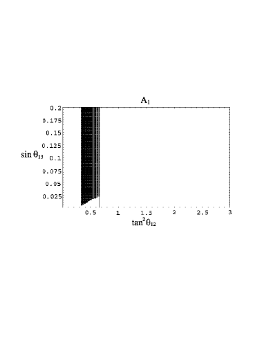
Figure 4: Scatter plot of $\sin\theta_{13}$ versus $\tan^{2}\theta_{12}$ in the case of $\kappa=2\overline{\omega}=0.07$.

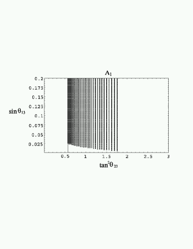
Figure 5: Scatter plot of $\sin\theta_{13}$ versus $\tan^{2}\theta_{23}$ in the case of $\kappa=2\overline{\omega}=0.07$.

In order to estimate the effect of $\overline{\omega}$ and $\overline{\epsilon}$, we consider the case in which the charged lepton mass matrix has small off-diagonal components. Suppose that the two zeros in eq.(16) is still preserved for the neutrino sector. The typical model of the charged lepton is the Georgi-Jarlskog texture [21], in which the charged lepton mass matrix $M_{E}$ is given as

$$M_{E}\simeq\ \left(\matrix{0&\sqrt{m_{e}m_{\mu}}&0\cr\sqrt{m_{e}m_{\mu}}&m_{\mu}&\sqrt{m_{e}m_{\tau}}\cr 0&\sqrt{m_{e}m_{\tau}}&m_{\tau}\cr}\right)\ ,$$ (21)

where each matrix element is written in terms of the charged lepton masses, and phases are neglected for simplicity. This matrix is diagonalized by the unitary matrix $U_{E}$, in which the mixing between the first and second families is $\sqrt{\frac{m_{e}}{m_{\mu}}}\simeq 0.07$ and the mixing between the second and third families is $\sqrt{\frac{m_{e}}{m_{\tau}}}\simeq 0.02$. Since the neutrino mass matrix is still the texture $A_{1}$, it turns to

$$M_{\nu}\sim\ \ \left(\matrix{\kappa^{2}&\kappa&\lambda\cr\kappa&1&1\cr\lambda&1&1\cr}\right)\ ,$$ (22)

in the diagonal basis of the charged lepton mass matrix. Here only the leading mixing term of $\kappa=\sqrt{\frac{m_{e}}{m_{\mu}}}$ is taken.

By using the texture of the neutrinos in eq.(22), we show our results of the allowed region of $\sin\theta_{13}$ versus $\tan^{2}\theta_{12}$ and $\tan^{2}\theta_{23}$ in Fig.4 and Fig.5, respectively. These results should be compared with the ones in Fig.2 and Fig.3. It is noticed that the lower bound of $\sin\theta_{13}$ considerably comes down due to the correction $\kappa$. The small $U_{e3}$ of $5\times 10^{-3}$ is allowed.

4 Summary

We have discussed $|U_{e3}|$ in the models, in which the samll $|U_{e3}|$ is predicted. The first one is the model in which the bi-maximal mixing is realized at the symmetric limit. The second one is the texture zeros of the neutrino mass matrix. In the first model, $|U_{e3}|=0.03\sim 0.2$ is predicted. In the second model, the lower bound of $|U_{e3}|$ is given as $0.05$, which considerably depends on $\tan^{2}\theta_{12}$ and $\tan^{2}\theta_{23}$. We have investigated the stability of these predictions by taking account of small corrections, which may come from radiative corrections or off-diagonal elements of the charged lepton mass matrix. The lower bound of $|U_{e3}|$ comes down significantly in the case of $\overline{\omega}\gg 0.01$, while $\overline{\epsilon}$ is rather insensitive to $|U_{e3}|$. The measurement of $|U_{e3}|$ will be an important test of the texture zeros in the future.

This talk is based on the reserach work with M. Honda and S. Kaneko. The research was supported by the Grant-in-Aid for Science Research, Ministry of Education, Science and Culture, Japan(No.12047220).

References

- [1] Super-Kamiokande Collaboration, Y. Fukuda et al, Phys. Rev. Lett. 81 (1998) 1562; ibid. 82 (1999) 2644; ibid. 82 (1999) 5194.
- [2] Super-Kamiokande Collaboration, S. Fukuda et al. Phys. Rev. Lett. 86, 5651; 5656 (2001).
-
[3]
SNO Collaboration: Q. R. Ahmad et al.,
Phys. Rev. Lett. 87 (2001) 071301;
nucl-ex/0204008, 0204009. - [4] KamLAND Collaboration, K. Eguchi et al., hep-ex/0212021.
-
[5]
G. L. Fogli, E. Lisi, M. Marrone, D. Montanino, A. Palazzo
and A.M. Rotunno, hep-ph/0212127;
J. N. Bahcall, M. C. Gonzalez-Garcia and C. Pea-Garay, JHEP 0302 (2003) 009;
M. Maltoni, T. Schwetz and J.W.F. Valle, hep-ph/0212129;
P.C. Holanda and A. Yu. Smirnov, hep-ph/0212270;
V. Barger and D. Marfatia, hep-ph/0212126. - [6] CHOOZ Collaboration, M. Apollonio et al., Phys. Lett. B466 (1999) 415.
-
[7]
J. Sato and T. Yanagida, Phys. Lett. B430 (1998) 123;
C.H. Albright, K.S. Babu and S.M. Barr, Phys. Rev. Lett. 81 (1998) 1167;
J. K. Elwood, N. Irges and P. Ramond, Phys. Rev. Lett. 81 (1998) 5064;
M. Bando and T. Kugo, Prog. Theor. Phys. 101 (1999)1313. -
[8]
H. Fritzsch and Z. Xing, Phys. Lett. B372 (1996) 265;
ibid. B440 (1998) 313;
M. Fukugita, M. Tanimoto and T. Yanagida, Phys. Rev. D57 (1998) 4429;
M. Tanimoto, Phys. Rev. D59 (1999) 017304;
M. Tanimoto, T. Watari and T. Yanagida, Phys. Lett. B461 (1999) 345. -
[9]
A. Zee, Phys. Lett. B93 (1980) 389; B161 (1985) 141;
L. Wolfenstein, Nucl. Phys. B175 (1980) 92;
S. T. Petcov, Phys. Lett. B115 (1982) 401;
C. Jarlskog, M. Matsuda, S. Skadhauge and M. Tanimoto, Phys. Lett. B449 (1999) 240;
P. H. Frampton and S. Glashow, Phys. Lett. B461 (1999) 95. -
[10]
L. J. Hall, H. Murayama and N. Weiner, Phys. Rev. Lett. 84
(2000) 2572;
N. Haba and H. Murayama, Phys. Rev. D63 (2001) 053010. - [11] C. Giunti and M. Tanimoto, Phys. Rev. D66 (2002) 053013; ibid. 113006.
- [12] H. Nishiura, K. Matsuda and T. Fukuyama, Phys. Rev. D60 (1999) 013006.
- [13] E. K. Akhmedov, G. C. Branco, M. N. Rebelo, Phys. Rev. Lett. 84 (2000) 3535.
- [14] S.K. Kang and C.S. Kim, Phys. Rev. D63 (2001) 113010.
- [15] P.H. Frampton, S.L. Glashow and D. Marfatia, Phys. Lett. B536 (2002) 79.
- [16] Z. Xing, Phys. Lett. B530 (2002) 159.
- [17] W. Guo and Z. Xing, hep-ph/0212142.
- [18] R. Barbieri, T. Hambye and A. Romanino, hep-ph/0302118.
- [19] M. Bando and M. Obara, hep-ph/0212242, 0302034.
- [20] Z. Maki, M. Nakagawa and S. Sakata, Prog. Theor. Phys. 28 (1962) 870.
- [21] H. Georgi and C. Jarlskog, Phys. Lett. B86 (1979) 297.