TUM-HEP-510/03

DESY 03-065

Running Neutrino Masses, Mixings and CP Phases: Analytical Results and Phenomenological Consequences

Stefan Antusch, Jörn Kersten, Manfred Lindner

Physik-Department T30, Technische Universität München
James-Franck-Straße, 85748 Garching, Germany

Michael Ratz

Deutsches Elektronensynchrotron DESY
22603 Hamburg, Germany

We derive simple analytical formulae for the renormalization group running of neutrino masses, leptonic mixing angles and CP phases, which allow an easy understanding of the running. Particularly for a small angle $\theta_{13}$ the expressions become very compact, even when non-vanishing CP phases are present. Using these equations we investigate: (i) the influence of Dirac and Majorana phases on the evolution of all parameters, (ii) the implications of running neutrino parameters for leptogenesis, (iii) changes of the mass bounds from WMAP and neutrinoless double $\beta$ decay experiments, relevant for high-energy mass models, (iv) the size of radiative corrections to $\theta_{13}$ and $\theta_{23}$ and implications for future precision measurements.

1 Introduction

The Standard Model (SM) agrees very well with experiments and the only solid evidence for new physics consists in the observation of neutrino masses. Compared to quarks and charged leptons they are tiny, for which the see-saw mechanism [1, 2, 3, 4] provides an attractive explanation. The parameters which enter into the neutrino mass matrix usually stem from model predictions at high energy scales, such as the scale $M_{\mathrm{GUT}}$ of grand unification. The measurements and bounds for neutrino masses and lepton mixings, on the other hand, determine the parameters at low energy. The high- and low-energy parameters are related by the renormalization group (RG) evolution, so that low-energy data yield only indirect restrictions for mass models or other high-energy mechanisms like leptogenesis [5]. It is well-known that the model independent RG evolution between low energy and the lowest see-saw scale can have large effects on the leptonic mixing angles and on the mass squared differences, in particular if the neutrinos have quasi-degenerate masses [6, 7, 8, 9, 10, 11, 12, 13, 14, 15, 16, 17, 18, 19, 20, 21, 22, 23]. RG effects may even serve as an explanation for the discrepancy between the mixings in the quark and the lepton sector [24].

The RG equations (RGEs) for the neutrino mass operator and for all the other parameters of the theory have to be solved simultaneously. The mixing angles, phases and mass eigenvalues can then be extracted from the evolved mass matrices. Both steps are, however, non-trivial and can only be performed numerically in practice. In order to determine the change of the parameters under the RG flow in a qualitative and, to a reasonable accuracy, also quantitative way, it is useful to derive analytical formulae for the running of the masses, mixing angles and phases. This was done in [10] assuming CP conservation and in [11] for the general case. We modify the derivation of [11] by a step which simplifies the formulae that arise after explicitly writing out the dependence on the mixing parameters. These results are exact, and they make it easier to derive simple approximations in the limit of small $\theta_{13}$. These approximations are very useful in understanding the RG evolution of the phases and the phase dependence of the evolution of other parameters. For example, we find that the phases show significant running. Consequently, vanishing phases at low energy appear unnatural unless exact CP conservation is a boundary condition at high energy, which seems unlikely, since the CP phase in the quark sector is sizable. The presence of CP phases at low energies has significant impact on observations [25, 26, 27].

The outline for the paper is: In Sec. 2 we present analytical formulae for the RG evolution of the neutrino masses, leptonic mixing angles and phases, where an expansion in the small angle $\theta_{13}$ is performed. This leads to very simple and in most cases accurate formulae which are compared with numerical results. Sec. 3 is devoted to phenomenological consequences for leptogenesis, the WMAP bound, the effective neutrino mass relevant for neutrinoless double beta decay and precision measurements of $\theta_{13}$ and $\theta_{23}$.

2 RG Evolution of Leptonic Mixing Parameters and Neutrino Masses

In this study, we will focus on neutrino masses which can be described by the lowest-dimensional neutrino mass operator compatible with the gauge symmetries of the SM. This operator reads in the SM

$$\mathscr{L}_{\kappa}=\frac{1}{4}\kappa_{gf}\,\overline{\ell_{\mathrm{L}}^{\mathrm{C}}}^{g}_{c}\varepsilon^{cd}\phi_{d}\,\,\ell_{\mathrm{L}b}^{f}\varepsilon^{ba}\phi_{a}+\text{h.c.}\;,$$ (1)

and in its minimal supersymmetric extension, the MSSM,

$$\mathscr{L}_{\kappa}^{\mathrm{MSSM}}\,=\,\mathscr{W}_{\mathrm{\kappa}}\big{|}_{\theta\theta}+\text{h.c.}=-\tfrac{1}{4}{\kappa}_{gf}\,\mathbb{l}^{g}_{c}\varepsilon^{cd}\mathbb{h}^{(2)}_{d}\,\,\mathbb{l}_{b}^{f}\varepsilon^{ba}\mathbb{h}^{(2)}_{a}\big{|}_{\theta\theta}+\text{h.c.}\;.$$ (2)

$\kappa_{gf}$ has mass dimension $-1$ and is symmetric under interchange of the generation indices $f$ and $g$, $\varepsilon$ is the totally antisymmetric tensor in 2 dimensions, and $\ell_{\mathrm{L}}^{\mathrm{C}}$ is the charge conjugate of a lepton doublet. $a,b,c,d\in\{1,2\}$ are $\mathrm{SU}(2)_{\mathrm{L}}$ indices. The double-stroke letters $\mathbb{l}$ and $\mathbb{h}$ denote lepton doublets and the up-type Higgs superfield in the MSSM. After electroweak (EW) symmetry breaking, a Majorana neutrino mass matrix proportional to $\kappa$ emerges as illustrated in Fig. 1.

$\vbox{\hbox{\includegraphics[scale={1}]{KappaSM.eps}}}\xrightarrow[\mbox{{\small breaking}}]{\mbox{{\small EW symmetry}}}\vbox{\hbox{\includegraphics[scale={1}]{KappaEWSB.eps}}}$

Figure 1: Vertex from the dimension 5 operator which yields a Majorana mass matrix for the light neutrinos.

The above mass operator provides a rather model-independent way to introduce neutrino masses as there are many possibilities to realize it radiatively or at tree-level within a renormalizable theory (see e.g. [28]). The tree-level realizations from integrating out heavy singlet fermions and/or Higgs triplets naturally appear for instance in left-right-symmetric extensions of the SM or MSSM and are usually referred to as type I and type II see-saw mechanisms.

The energy dependence of the effective neutrino mass matrix below the scale where the operator is generated (which we will call $M_{1}$ in the following) is described by its RGE. At the one-loop level, this equation is given by [29, 30, 31, 32]

$$16\pi^{2}\,\frac{\mathrm{d}\kappa}{\mathrm{d}t}\,=\,C\,(Y_{e}^{\dagger}Y_{e})^{T}\,\kappa+C\,\kappa\,(Y_{e}^{\dagger}Y_{e})+\alpha\,\kappa\;,$$ (3)

where $t=\ln(\mu/\mu_{0})$ and $\mu$ is the renormalization scale and where

$$C = 1\hphantom{-\frac{3}{2}}\;\;\text{in the MSSM}\;,$$

$$C = -\frac{3}{2}\hphantom{1}\;\;\text{in the SM}\;.$$ (4)

In the SM and in the MSSM, $\alpha$ reads

$$\alpha_{\mathrm{SM}} = -3g_{2}^{2}+2(y_{\tau}^{2}+y_{\mu}^{2}+y_{e}^{2})+6\left(y_{t}^{2}+y_{b}^{2}+y_{c}^{2}+y_{s}^{2}+y_{d}^{2}+y_{u}^{2}\right)+\lambda\;,$$ (5a)

$$\alpha_{\mathrm{MSSM}} = -\frac{6}{5}g_{1}^{2}-6g_{2}^{2}+6\left(y_{t}^{2}+y_{c}^{2}+y_{u}^{2}\right)\;.$$ (5b)

Here $Y_{f}$ ($f\in\{e,d,u\}$) represent the Yukawa coupling matrices of the charged leptons, down- and up-type quarks, respectively, $g_{i}$ denote the gauge couplings and $\lambda$ the Higgs self-coupling in the SM. We work in the basis where $Y_{e}$ is diagonal.

The parameters of interest are the masses, which are proportional to the eigenvalues of $\kappa$ and defined to be non-negative, as well as the mixing angles and physical phases of the MNS matrix [34]

$$U_{\mathrm{MNS}} = V(\theta_{12},\theta_{13},\theta_{23},\delta)\,\operatorname{diag}(e^{-\mathrm{i}\varphi_{1}/2},e^{-\mathrm{i}\varphi_{2}/2},1)\;,$$ (6)

which diagonalizes $\kappa$ in this basis. $V$ is the leptonic analogon to the CKM matrix in the quark sector. The parametrization we use will be explained in more detail in App. A. Currently, we learn from experiments that there occur two oscillations with mass squared differences $\Delta m^{2}_{\mathrm{sol}}$ and $\Delta m^{2}_{\mathrm{atm}}$ and corresponding mixing angles $\theta_{12}$ and $\theta_{23}$, respectively. For the third mixing angle $\theta_{13}$ and the absolute scale of light neutrino masses, there are only upper bounds at the moment (see Tab. 1 for the present status).

	Best-fit value	Range (for $\theta_{ij}\in[0^{\circ},45^{\circ}]$)	C.L.
$\theta_{12}$ [${\>}^{\circ}$]	$32.6$	$25.6-42.0$	$99\%\;(3\sigma)$
$\theta_{23}$ [${\>}^{\circ}$]	$45.0$	$33.2-45.0$	$99\%\;(3\sigma)$
$\theta_{13}$ [${\>}^{\circ}$]	$-$	$0.0-9.2$	$90\%$
$\Delta m^{2}_{\mathrm{sol}}$ [eV2]	$7.3\cdot 10^{-5}$	$4\cdot 10^{-5}-2.8\cdot 10^{-4}$	$99\%\;(3\sigma)$
$|\Delta m^{2}_{\mathrm{atm}}|$ [eV2]	$2.5\cdot 10^{-3}$	$1.2\cdot 10^{-3}-5\cdot 10^{-3}$	$99\%\;(3\sigma)$

Table 1: Experimental data for the neutrino mixing angles and mass squared differences. For the solar angle $\theta_{12}$ and the solar mass squared difference, the LMA solution as confirmed by KamLAND is shown. The results stem from the analysis [35] of the recent KamLAND and the SNO data, the Super-Kamiokande atmospheric data [36] and the CHOOZ experiment [37].

2.1 The Analytical Formulae

In this section, we present explicit RGEs for the physical parameters. They determine the slope of the RG evolution at a given energy scale and thus yield an insight into the RG behavior. The derivation will be discussed in App. B. Note that a naive linear interpolation, i.e.  assuming the right-hand sides of the equations to be constant, will not always give the correct RG evolution. As we will show later, this is mainly due to large changes of $\theta_{12}$ and the mass squared differences. In the following, we will neglect ${y_{e}}$ and ${y_{\mu}}$ against $y_{\tau}$ and introduce the abbreviation

$$\zeta\,:=\,\frac{\Delta m^{2}_{\mathrm{sol}}}{\Delta m^{2}_{\mathrm{atm}}}\;,$$ (7)

whose LMA best-fit value is about 0.03. In order to keep the expressions short, we will only show the leading terms in an expansion in the small angle $\theta_{13}$ for the mixing parameters. In almost all cases they are sufficient for understanding the features of the RG evolution. In all cases except for the running of the Dirac phase $\delta$, the limit $\theta_{13}\to 0$ causes no difficulties, the subtleties arising for $\delta$ will be discussed in Sec. 2.4.1. We furthermore define $m_{i}(t):=v^{2}\,\kappa_{i}(t)/4$ with $v=246\,\mathrm{GeV}$ in the SM or $v=246\,\mathrm{GeV}\cdot\sin\beta$ in the MSSM and, as usual, $\Delta m^{2}_{\mathrm{sol}}:=m_{2}^{2}-m_{1}^{2}$ and $\Delta m^{2}_{\mathrm{atm}}:=m_{3}^{2}-m_{2}^{2}$. Note that our formulae cannot be applied if one of the mass squared differences vanishes. For a discussion of RG effects in this case, see e.g. [7, 8, 9, 22, 38]. With these conventions, we obtain the following analytical expressions for the mixing angles:

$$\dot{\theta}_{12} = -\frac{Cy_{\tau}^{2}}{32\pi^{2}}\,\sin 2\theta_{12}\,s_{23}^{2}\,\frac{|{m_{1}}\,e^{\mathrm{i}\varphi_{1}}+{m_{2}}\,e^{\mathrm{i}\varphi_{2}}|^{2}}{\Delta m^{2}_{\mathrm{sol}}}+\mathscr{O}(\theta_{13})\;,$$ (8)

$$\dot{\theta}_{13} = \frac{Cy_{\tau}^{2}}{32\pi^{2}}\,\sin 2\theta_{12}\,\sin 2\theta_{23}\,\frac{m_{3}}{\Delta m^{2}_{\mathrm{atm}}\left(1+\zeta\right)}\times$$ (9)

$$\quad\times\left[m_{1}\cos(\varphi_{1}-\delta)-\left(1+\zeta\right)m_{2}\,\cos(\varphi_{2}-\delta)-\zeta m_{3}\,\cos\delta\right]+\mathscr{O}(\theta_{13})\;,$$

$$\dot{\theta}_{23} = -\frac{Cy_{\tau}^{2}}{32\pi^{2}}\,\sin 2\theta_{23}\,\frac{1}{\Delta m^{2}_{\mathrm{atm}}}\left[c_{12}^{2}\,|m_{2}\,e^{\mathrm{i}\varphi_{2}}+m_{3}|^{2}+s_{12}^{2}\,\frac{|m_{1}\,e^{\mathrm{i}\varphi_{1}}+m_{3}|^{2}}{1+\zeta}\right]$$ (10)

$${}+\mathscr{O}(\theta_{13})\;.$$

Note that in order to apply Eq. (9) to the case $\theta_{13}=0$, where $\delta$ is undefined, the analytic continuation of the latter, which will be given in Eq. (25), has to be inserted. The $\mathscr{O}(\theta_{13})$ terms in the above RGEs can become important if $\theta_{13}$ is not too small and in particular if cancellations appear in the leading terms. For example, this is the case for $|\varphi_{1}-\varphi_{2}|=\pi$ in (8), as we will discuss below in more detail. The RGE for the Dirac phase is given by

$$\dot{\delta}\,=\,\frac{Cy_{\tau}^{2}}{32\pi^{2}}\frac{\delta^{(-1)}}{\theta_{13}}+\frac{Cy_{\tau}^{2}}{8\pi^{2}}\delta^{(0)}+\mathscr{O}(\theta_{13})\;,$$ (11)

where

$$\delta^{(-1)} = \sin 2\theta_{12}\,\sin 2\theta_{23}\,\frac{m_{3}}{\Delta m^{2}_{\mathrm{atm}}\left(1+\zeta\right)}\times$$ (12a)

$$\quad\times\left[m_{1}\sin(\varphi_{1}-\delta)-\left(1+\zeta\right)m_{2}\,\sin(\varphi_{2}-\delta)+\zeta m_{3}\,\sin\delta\right]\;,$$

$$\delta^{(0)} = \frac{m_{1}m_{2}\,s_{23}^{2}\,\sin(\varphi_{1}-\varphi_{2})}{\Delta m^{2}_{\mathrm{sol}}}$$ (12b)

$${}+m_{3}\,s_{12}^{2}\left[\frac{m_{1}\,\cos 2\theta_{23}\,\sin\varphi_{1}}{\Delta m^{2}_{\mathrm{atm}}(1+\zeta)}+\frac{m_{2}\,c_{23}^{2}\,\sin(2\delta-\varphi_{2})}{\Delta m^{2}_{\mathrm{atm}}}\right]$$

$${}+m_{3}\,c_{12}^{2}\left[\frac{m_{1}\,c_{23}^{2}\,\sin(2\delta-\varphi_{1})}{\Delta m^{2}_{\mathrm{atm}}(1+\zeta)}+\frac{m_{2}\,\cos 2\theta_{23}\,\sin\varphi_{2}}{\Delta m^{2}_{\mathrm{atm}}}\right]\;.$$

For the physical Majorana phases, we obtain

$$\dot{\varphi}_{1} = \frac{Cy_{\tau}^{2}}{4\pi^{2}}\left\{m_{3}\,\cos 2\theta_{23}\,\frac{m_{1}s_{12}^{2}\,\sin\varphi_{1}+\left(1+\zeta\right)m_{2}\,c_{12}^{2}\,\sin\varphi_{2}}{\Delta m^{2}_{\mathrm{atm}}\left(1+\zeta\right)}\right.$$ (13)

$$\hphantom{\frac{Cy_{\tau}^{2}}{4\pi^{2}}\left\{\right.}\left.{}+\frac{m_{1}m_{2}\,c_{12}^{2}\,s_{23}^{2}\,\sin(\varphi_{1}-\varphi_{2})}{\Delta m^{2}_{\mathrm{sol}}}\right\}+\mathscr{O}(\theta_{13})\;,$$

$$\dot{\varphi}_{2} = \frac{Cy_{\tau}^{2}}{4\pi^{2}}\left\{m_{3}\,\cos 2\theta_{23}\,\frac{m_{1}s_{12}^{2}\,\sin\varphi_{1}+\left(1+\zeta\right)m_{2}\,c_{12}^{2}\sin\varphi_{2}}{\Delta m^{2}_{\mathrm{atm}}\left(1+\zeta\right)}\right.$$ (14)

$$\hphantom{\frac{Cy_{\tau}^{2}}{4\pi^{2}}\left\{\right.}\left.{}+\frac{m_{1}m_{2}\,s_{12}^{2}\,s_{23}^{2}\,\sin(\varphi_{1}-\varphi_{2})}{\Delta m^{2}_{\mathrm{sol}}}\right\}+\mathscr{O}(\theta_{13})\;.$$

We would like to emphasize that the above expressions do not contain expansions in $\zeta$, i.e. their $\zeta$ dependence is exact. In many cases, they can be further simplified by neglecting $\zeta$ against 1 without losing much accuracy. Note that singularities can appear in the $\mathscr{O}(\theta_{13})$-terms at points in parameter space where the phases are not well-defined. For the masses, the results for $y_{e}=y_{\mu}=0$ but arbitrary $\theta_{13}$ are

$$16\pi^{2}\,\dot{m}_{1} = \left[\alpha+Cy_{\tau}^{2}\left(2s_{12}^{2}\,s_{23}^{2}+F_{1}\right)\right]m_{1}\;,$$ (15a)

$$16\pi^{2}\,\dot{m}_{2} = \left[\alpha+Cy_{\tau}^{2}\left(2c_{12}^{2}\,s_{23}^{2}+F_{2}\right)\right]m_{2}\;,$$ (15b)

$$16\pi^{2}\,\dot{m}_{3} = \left[\alpha+2Cy_{\tau}^{2}\,c_{13}^{2}\,c_{23}^{2}\right]m_{3}\;,$$ (15c)

where $F_{1}$ and $F_{2}$ contain terms proportional to $\sin\theta_{13}$,

$$F_{1} = -s_{13}\,\sin 2\theta_{12}\,\sin 2\theta_{23}\,\cos\delta+2s_{13}^{2}\,c_{12}^{2}\,c_{23}^{2}\;,$$ (16a)

$$F_{2} = s_{13}\,\sin 2\theta_{12}\,\sin 2\theta_{23}\,\cos\delta+2s_{13}^{2}\,s_{12}^{2}\,c_{23}^{2}\;.$$ (16b)

These formulae can be translated into RGEs for the mass squared differences,

$$\!8\pi^{2}\,\frac{\mathrm{d}}{\mathrm{d}t}\Delta m_{\mathrm{sol}}^{2}\, = \!\alpha\,\Delta m_{\mathrm{sol}}^{2}+Cy_{\tau}^{2}\left[2s_{23}^{2}\left(m_{2}^{2}\,c_{12}^{2}-m_{1}^{2}\,s_{12}^{2}\right)+F_{\mathrm{sol}}\right]\;,$$ (17a)

$$8\pi^{2}\,\frac{\mathrm{d}}{\mathrm{d}t}\Delta m_{\mathrm{atm}}^{2} = \!\alpha\,\Delta m_{\mathrm{atm}}^{2}+Cy_{\tau}^{2}\left[2m_{3}^{2}\,c_{13}^{2}\,c_{23}^{2}-2m_{2}^{2}\,c_{12}^{2}\,s_{23}^{2}+F_{\mathrm{atm}}\right]\;,$$ (17b)

where

$$F_{\mathrm{sol}} = \left(m_{1}^{2}+m_{2}^{2}\right)s_{13}\,\sin 2\theta_{12}\,\sin 2\theta_{23}\,\cos\delta$$ (18a)

$${}+2s_{13}^{2}\,c_{23}^{2}\left(m_{2}^{2}\,s_{12}^{2}-m_{1}^{2}\,c_{12}^{2}\right)\;,$$

$$F_{\mathrm{atm}} = -m_{2}^{2}\,s_{13}\,\sin 2\theta_{12}\,\sin 2\theta_{23}\,\cos\delta-2m_{2}^{2}\,s_{13}^{2}\,s_{12}^{2}\,c_{23}^{2}\;.$$ (18b)

2.2 Generic Enhancement and Suppression Factors

From Eqs. (8)–(14) it follows that there are generic enhancement and suppression factors for the RG evolution of the mixing parameters, depending on whether the mass scheme is hierarchical, partially degenerate or nearly degenerate. We have listed these factors in the approximation of small $\theta_{13}$ in Tab. 2. They can be compensated by cancellations due to a special alignment of the phases. For example, an opposite CP parity of the first and second mass eigenstate, i.e.  $|\varphi_{1}-\varphi_{2}|=\pi$, results in a maximal suppression of the running of the solar mixing angle, which has been pointed out earlier in papers like [11, 39, 13, 17]. Nevertheless, Tab. 2 allows to determine which angles or phases have a potential for a strong RG evolution. Obviously, the expressions for $\dot{\delta}$ are not applicable for $\theta_{13}=0$. This special case will be discussed at the end of Sec. 2.4.1.

	$\dot{\theta}_{12}$	$\dot{\theta}_{13}$	$\dot{\theta}_{23}$	$\dot{\delta}$	$\dot{\varphi}_{i}$
n.h.	1	$\displaystyle\sqrt{\zeta}$	$1$	$\displaystyle\sqrt{\zeta}\,\theta_{13}^{-1}$	$\displaystyle\sqrt{\zeta}$
p.d.(n.)	$\displaystyle\frac{m_{1}^{2}}{\Delta m^{2}_{\mathrm{sol}}}$	$\displaystyle\frac{m_{1}}{\sqrt{\Delta m^{2}_{\mathrm{atm}}}}$	$1$	$\displaystyle\frac{m_{1}}{\sqrt{\Delta m^{2}_{\mathrm{atm}}}}\theta_{13}^{-1}+\frac{m_{1}^{2}}{\Delta m^{2}_{\mathrm{sol}}}$	$\displaystyle\frac{m_{1}^{2}}{\Delta m^{2}_{\mathrm{sol}}}$
i.h.	$\zeta^{-1}$	$\mathscr{O}(\theta_{13})$	$1$	$\zeta^{-1}$	$\displaystyle\zeta^{-1}$
p.d.(i.)	$\zeta^{-1}$	$\displaystyle\frac{m_{3}}{\sqrt{\Delta m^{2}_{\mathrm{atm}}}}$	$1$	$\displaystyle\frac{m_{3}}{\sqrt{\Delta m^{2}_{\mathrm{atm}}}}\theta_{13}^{-1}+\zeta^{-1}$	$\displaystyle\zeta^{-1}$
d.	$\displaystyle\frac{m^{2}}{\Delta m^{2}_{\mathrm{sol}}}$	$\displaystyle\frac{m^{2}}{\Delta m^{2}_{\mathrm{atm}}}$	$\displaystyle\frac{m^{2}}{\Delta m^{2}_{\mathrm{atm}}}$	$\displaystyle\frac{m^{2}}{\Delta m^{2}_{\mathrm{atm}}}\theta_{13}^{-1}+\displaystyle\frac{m^{2}}{\Delta m^{2}_{\mathrm{sol}}}$	$\displaystyle\frac{m^{2}}{\Delta m^{2}_{\mathrm{sol}}}$

Table 2: Generic enhancement and suppression factors for the RG evolution of the mixing parameters. A ‘1’ indicates that there is no generic enhancement or suppression. ‘n.h.’ and ‘p.d.(n.)’ denote the hierarchical and partially degenerate mass spectrum in the case of a normal hierarchy, i.e. $m_{1}^{2}\ll\Delta m_{\mathrm{sol}}^{2}$ or $\Delta m^{2}_{\mathrm{sol}}\ll m_{1}^{2}\lesssim\Delta m_{\mathrm{atm}}^{2}$. ‘i.h.’ and ‘p.d.(i.)’ denote the analogous spectra in the inverted case, i.e.  $m_{3}^{2}\ll\Delta m_{\mathrm{sol}}^{2}$ or $\Delta m^{2}_{\mathrm{sol}}\ll m_{3}^{2}\lesssim\Delta m_{\mathrm{atm}}^{2}$. Finally, ‘d.’ means nearly degenerate masses, $\Delta m^{2}_{\mathrm{atm}}\ll m_{1}^{2}\sim m_{2}^{2}\sim m_{3}^{2}\sim m^{2}$.

Let us consider some numerical values in order to estimate the size of RG effects. The SM $\tau$ Yukawa coupling is $y_{\tau}^{\mathrm{SM}}=\frac{\sqrt{2}}{v}m_{\tau}\approx 0.01$. Thus, the typical factor in the formulae for the mixing angles and phases amounts to

$$\frac{3y_{\tau}^{2}}{64\pi^{2}}\approx 0.5\cdot 10^{-6}\;.$$ (19)

In the MSSM it changes to

$$\frac{y_{\tau}^{2}}{32\pi^{2}}\approx 0.3\cdot 10^{-6}\left(1+\tan^{2}\beta\right)\;.$$ (20)

If the running was purely logarithmic, it would yield a factor of

$$\ln\frac{M_{1}}{M_{Z}}\approx\ln\frac{10^{13}}{10^{2}}\approx 25$$ (21)

for $M_{1}=10^{13}\,\mathrm{GeV}$. If we assume that the solar and atmospheric angle are large and that the phases do not cause excessive cancellations, then multiplying the above two contributions with the enhancement factor $\Gamma_{\mathrm{enh}}$ from Tab. 2 yields a rough estimate for the change of the angles and phases due to the RG evolution,

$$\Delta_{\mathrm{RG}}\sim 10^{-5}\left(1+\tan^{2}\beta\right)\Gamma_{\mathrm{enh}}\;.$$ (22)

Of course the factor $1+\tan^{2}\beta$ has to be omitted in the SM. It is immediately clear that even in the MSSM with very large $\tan\beta$ no significant change occurs if the enhancement factor is 1 or less – except maybe for $\theta_{13}$, where even a change by $1^{\circ}$ could be interesting. However, for quasi-degenerate neutrinos large enhancement factors are possible. As an example, let us estimate the size of the absolute neutrino mass scale (the ‘amount of degeneracy’) needed for a sizable RG change of $\theta_{12}$, say $0.1\approx 6^{\circ}$. In the SM, this requires $\Gamma_{\mathrm{enh}}\sim 10^{4}$, corresponding to a neutrino mass of the order of $1\,\mathrm{eV}$, which is excluded by WMAP and double beta decay experiments. On the other hand, in the MSSM this mass scale can easily be lowered to about $0.1\,\mathrm{eV}$ with $\tan\beta$ as small as 8.

2.3 Discussion and Comparison with Numerical Results

We now study in detail the running of the mixing angles and masses, in particular the influence of the phases. The RG evolution of the phases will be studied separately in Sec. 2.4. We solve the RGEs for the neutrino mass operator and for the other parameters numerically and compare the results with those obtained from the analytical formulae of Sec. 2.1. For the numerics we follow the ‘run and diagonalize’ procedure, i.e. we first compute the running of the mass matrix and then extract the evolving mass eigenvalues and mixing parameters. The algorithm used for this is described in App. A. As an example, we consider the MSSM with $\tan\beta=50$, a normal mass hierarchy for the neutrinos, $m_{1}=0.1\,\mathrm{eV}$ for the mass of the lightest neutrino, and a mass of about $120\,\mathrm{GeV}$ for the light Higgs. These boundary conditions are given at the electroweak scale, i.e.  we calculate the evolution from low to high energies. Below the SUSY-breaking scale, which we take to be $1.5\,\mathrm{TeV}$, we assume the SM to be valid as an effective theory and use the corresponding RGEs. Above, we apply the ones of the MSSM.

2.3.1 RG Evolution of $\boldsymbol{\theta_{12}}$

From Tab. 2, we see that the solar angle $\theta_{12}$ generically has the strongest RG effects among the mixing angles. The reason for this is the smallness of the solar mass squared difference associated with it, in particular compared to the atmospheric one, which leads to an enhanced running for quasi-degenerate neutrinos and for the case of an inverted mass hierarchy. Furthermore, it is known that in the MSSM the solar angle always increases when running down from $M_{1}$ for $\theta_{13}=0$ [20]. This is confirmed by our formula (8). From the term $|{m_{1}}\,e^{\mathrm{i}\varphi_{1}}+{m_{2}}\,e^{\mathrm{i}\varphi_{2}}|^{2}$ in Eq. (8), we see that a non-zero value of the difference $|\varphi_{1}-\varphi_{2}|$ of the Majorana phases damps the RG evolution. The damping becomes maximal if this difference equals $\pi$, which corresponds to an opposite CP parity of the mass eigenstates $m_{1}$ and $m_{2}$. This is in agreement with earlier studies, e.g. [11, 39, 13, 17].

Let us now compare the analytical approximation for $\dot{\theta}_{12}$ of Eq. (8) with the numerical solution for the running in the case of nearly degenerate masses, which is shown in Fig. 2 in detail. The dark-gray region shows the evolution with LMA best-fit values for the neutrino parameters, $\theta_{13}$ varying in the interval $[0^{\circ},9^{\circ}]$ and all CP phases equal to zero. The medium-gray regions show the evolution for $|\varphi_{1}-\varphi_{2}|\in\{0^{\circ},90^{\circ},180^{\circ},270^{\circ}\}$, $\theta_{13}\in[0^{\circ},9^{\circ}]$ and $\delta\in\{0^{\circ},90^{\circ},180^{\circ},270^{\circ}\}$, confirming the expectation of the damping influence of $\varphi_{1}$ and $\varphi_{2}$. The flat line at low energy stems from the SM running below $M_{\mathrm{SUSY}}$, which is negligible as we have seen earlier. Note that the numerics never yield negative values of $\theta_{12}$ due to the algorithm used for extracting the mixing parameters from the MNS matrix, which guarantees $0\leq\theta_{12}\leq 45^{\circ}$ (see App. A.3 for further details).

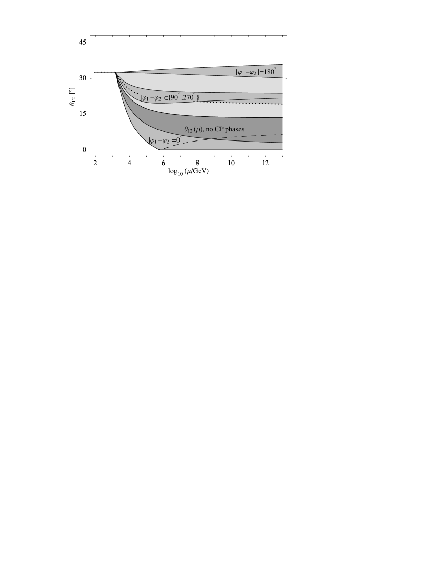
Figure 2: RG evolution of $\theta_{12}$ in the MSSM with $\tan\beta=50$, a normal mass hierarchy and $m_{1}=0.1\,\mathrm{eV}$. The dark-gray region shows the evolution with best-fit values for the neutrino parameters, $\theta_{13}\in[0^{\circ},9^{\circ}]$ and all CP phases equal to zero. The medium-gray regions show the evolution for $|\varphi_{1}-\varphi_{2}|=0^{\circ}$, $|\varphi_{1}-\varphi_{2}|\in\{90^{\circ},270^{\circ}\}$ and $|\varphi_{1}-\varphi_{2}|=180^{\circ}$. They emerge from varying $\theta_{13}\in[0^{\circ},9^{\circ}]$ and $\delta\in\{0^{\circ},90^{\circ},180^{\circ},270^{\circ}\}$. The light-gray regions can be reached by choosing specific values for the CP phases different from the ones listed above. The dashed line shows the RG evolution with $|\varphi_{1}-\varphi_{2}|=0$, $\theta_{13}=9^{\circ}$ and $\delta=180^{\circ}$. Note that for the numerics we use the convention where $\theta_{12}$ is restricted to the interval $[0^{\circ},45^{\circ}]$, so that the angle increases again after reaching 0. The dotted line shows the evolution with $|\varphi_{1}-\varphi_{2}|=90^{\circ}$ and $\theta_{13}=0^{\circ}$.

As can be seen from the relatively broad dark-gray band in the figure, the $\mathscr{O}(\theta_{13})$-term in the RGE is quite important here. The dominant part of this term is

$$\Upsilon = \frac{Cy_{\tau}^{2}}{32\pi^{2}}\frac{m_{2}+m_{1}}{m_{2}-m_{1}}\,\sin 2\theta_{23}\,\cos\frac{\varphi_{1}-\varphi_{2}}{2}\times$$ (23)

$$\quad{}\times\Bigl{(}\cos 2\theta_{12}\,\cos\delta\,\cos\frac{\varphi_{1}-\varphi_{2}}{2}+\sin\delta\,\sin\frac{\varphi_{1}-\varphi_{2}}{2}\Bigr{)}\cdot\theta_{13}\;.$$

Clearly, the RG evolution of $\theta_{12}$ is independent of the Dirac phase $\delta$ only in the approximation $\theta_{13}=0$. The largest running, where $\theta_{12}$ can even become zero, occurs for $\theta_{13}$ as large as possible ($9^{\circ}$), $\delta=\pi$ and $\varphi_{1}-\varphi_{2}=0$. In this case the leading and the next-to-leading term add up constructively. It is also interesting to observe that due to $\mathscr{O}(\theta_{13})$ effects $\theta_{12}$ can run to slightly larger values. The damping due to the Majorana phases is maximal in this case, which almost eliminates the leading term. Then, all the running comes from the next-to-leading term (23).

In the inverted scheme, $m_{1}\gg m_{2}-m_{1}$ always holds, so that large RG effects are generic, i.e.  always present except for the case of cancellations due to Majorana phases. For a normal mass hierarchy with a small $m_{1}$, the running of the solar mixing is of course rather insignificant.

Finally, we would like to emphasize that it is not appropriate to assume the right-hand sides of Eq. (8) and Eq. (23) to be constant in order to interpolate $\theta_{12}$ up to a high energy scale, since non-linear effects especially from the running of $\sin 2\theta_{12}$ and $\Delta m^{2}_{\mathrm{sol}}$ cannot be neglected here. This is easily seen from the curved lines in Fig. 2.

2.3.2 RG Evolution of $\boldsymbol{\theta_{13}}$

The analytical approximation for $\dot{\theta}_{13}$ is given in Eq. (9). As already pointed out, in order to apply it to the case $\theta_{13}=0$, where $\delta$ is undefined, the analytic continuation of the latter has to be inserted. It will be given in Eq. (25) in section 2.4.1, where the phases are treated in detail. The comparison with the numerical results in Fig. 3 shows that above $M_{\mathrm{SUSY}}$ the angle runs linearly on a logarithmic scale to a good approximation. Thus, using Eq. (9) with a constant right-hand side yields pretty accurate results. With $\varphi_{1}\neq\varphi_{2}$, significant RG effects can be expected for nearly degenerate masses. This is confirmed by the light-gray region in Fig. 3.

The fastest running occurs if $\varphi_{1}-\varphi_{2}=\pi$ and $\varphi_{1}-\delta\in\{0,\pi\}$, so that the terms proportional to $m_{1}$ and $m_{2}$ in the RGE are maximal and add up. Interestingly, cancellations between the first two terms in the second line of Eq. (9) appear for $\varphi_{1}=\varphi_{2}$, in particular if all phases are zero. If so, the leading contribution to the evolution of $\theta_{13}$ is suppressed by an additional factor of $\zeta$. This suppression is in agreement with earlier studies, for instance [39, 21], where it was discussed for the CP-conserving case $\varphi_{1}=\varphi_{2}=\pi$, which implies an opposite CP parity of $m_{3}$ compared to the other two mass eigenvalues. Such cancellations cannot occur for a strong normal mass hierarchy, since then the evolution is dominated by the term proportional to $m_{2}$ in Eq. (9).

Besides, $\theta_{13}$ runs towards smaller values in the MSSM with zero phases and a normal hierarchy, because $m_{1}<m_{2}$, so that the second line of the RGE is negative. This yields the dark-gray region in Fig. 3. As $\theta_{13}$ can always be made positive by a suitable redefinition of parameters, the sign of $\dot{\theta}_{13}$ is irrelevant for $\theta_{13}=0$.

For an inverted hierarchy, the situation is reversed, since $\Delta m^{2}_{\mathrm{atm}}$ is negative then. For a small $m_{3}$, the running is highly suppressed in this case, because the leading term is proportional to $m_{3}$. Then the dominant contribution comes from the $\mathscr{O}(\theta_{13})$-term unless $\theta_{13}$ is very small as well.

Future experiments will probably be able to probe $\sin^{2}2\theta_{13}$ down to $10^{-4}$, corresponding to $\theta_{13}\sim 5\cdot 10^{-3}\sim 0.3^{\circ}$. Consequently, even RG changes of this order of magnitude could be important, since a low-energy value smaller than the RG change would appear unnatural. This will be discussed in more detail in Sec. 3.3.

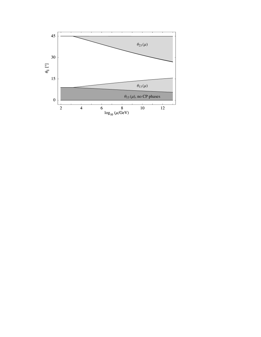
Figure 3: RG evolution of $\theta_{13}$ and $\theta_{23}$ in the MSSM with $\tan\beta=50$, a normal mass hierarchy and $m_{1}=0.1\,\mathrm{eV}$. The dark-gray region shows the evolution with best-fit values for the neutrino parameters, $\theta_{13}\in[0^{\circ},9^{\circ}]$ and all CP phases equal to zero. For the $\theta_{23}$ case, we just obtain a thick gray line at the bottom of the gray region. The light-gray regions show the evolution, which is possible, if arbitrary CP phases are allowed.

2.3.3 RG Evolution of $\boldsymbol{\theta_{23}}$

The analytical RGE for $\dot{\theta}_{23}$ can be found in Eq. (10). Again, the comparison with the numerical results (see Fig. 3) shows that to a good approximation the angle runs linearly on a logarithmic scale above $M_{\mathrm{SUSY}}$. The sign of $\Delta m^{2}_{\mathrm{atm}}$ is very important here. For a normal mass spectrum, the leading term is always negative in the MSSM, so that $\theta_{23}$ decreases with increasing energy, while for an inverse spectrum the situation is exactly reversed, so that $\theta_{23}$ becomes larger than $45^{\circ}$ if one starts with the LMA best-fit value at low energy.

From Eq. (10) we expect that switching on the phases $\varphi_{1}$ and $\varphi_{2}$ always reduces the running of $\theta_{23}$ for nearly degenerate masses. This is confirmed by the light-gray region in Fig. 3. The damping is much less severe for a hierarchical mass spectrum, since either $m_{1}$ and $m_{2}$ or $m_{3}$ are very small then. However, in these cases the running is generally expected to be rather insignificant, since according to Tab. 2 the enhancement factor is only 1.

2.3.4 RG Evolution of the Neutrino Mass Eigenvalues

The running of the mass eigenvalues is significant even in the SM or for strongly hierarchical neutrino masses due to the factor $\alpha$ in the RGEs (15). Clearly, the evolution is not directly dependent on the Majorana phases [11]. This can be understood from Eqs. (B.13) and (B.19), which show that only the moduli of the elements of the MNS matrix enter into $\dot{m}_{i}$. Besides, $\dot{m}_{3}$ does not depend on $\delta$, since only the moduli of the elements of the third column of the MNS matrix are relevant in this case. Of course, there is an indirect dependence on the phases, as these influence the running of the mixing angles.

Apart from the MSSM with large $\tan\beta$, the running of the mass eigenvalues is virtually independent of the mixing parameters, since $\alpha$ is usually much larger than $y_{\tau}^{2}$. In the SM, the Higgs mass influences the running via the self-coupling $\lambda$ – the heavier the Higgs, the larger the RG effects. Thus, except for large $\tan\beta$ in the MSSM, the running is given by a common scaling of the mass eigenvalues [17], which is obtained by neglecting $y_{\tau}$ and integrating Eq. (15),

$$m_{i}(t)\,\approx\,\exp\left[\frac{1}{16\pi^{2}}\int_{t_{0}}^{t}\mathrm{d}\tau\,\alpha(\tau)\right]\,m_{i}(t_{0})\,=:\,s(t,t_{0})\,m_{i}(t_{0})\;.$$ (24)

We plot $s$ in the SM and in the MSSM for various parameter combinations in Fig. 4. The three SM curves correspond to different Higgs masses in the current experimentally allowed region at 95% confidence level, $114\,\mathrm{GeV}\lesssim m_{H}\lesssim 200\,\mathrm{GeV}$ [40]. $m_{H}=180\,\mathrm{GeV}$ is the value for which the self-coupling $\lambda$ stays perturbative up to $10^{16}\,\mathrm{GeV}$, i.e. $\lambda\lesssim 1$, and $m_{H}=165\,\mathrm{GeV}$ is the minimal mass for which $\lambda$ is positive up to $10^{16}\,\mathrm{GeV}$, so that the vacuum is stable in this region (see e.g. [41, 42]). In the MSSM, we choose $m_{H}=120\,\mathrm{GeV}$ for the light Higgs mass, since the allowed range is further restricted by the upper limit at about $130\,\mathrm{GeV}$ here, and since it influences the evolution of the RG scaling only marginally as long as $M_{\mathrm{SUSY}}$ and $M_{Z}$ differ only by a few orders of magnitude. Moreover, further uncertainties due to threshold corrections and the unknown value of the SUSY-breaking scale can be equally important as the one due to the unknown Higgs mass. The RG enhancement of the masses is smallest if $\tan\beta\approx 10$.

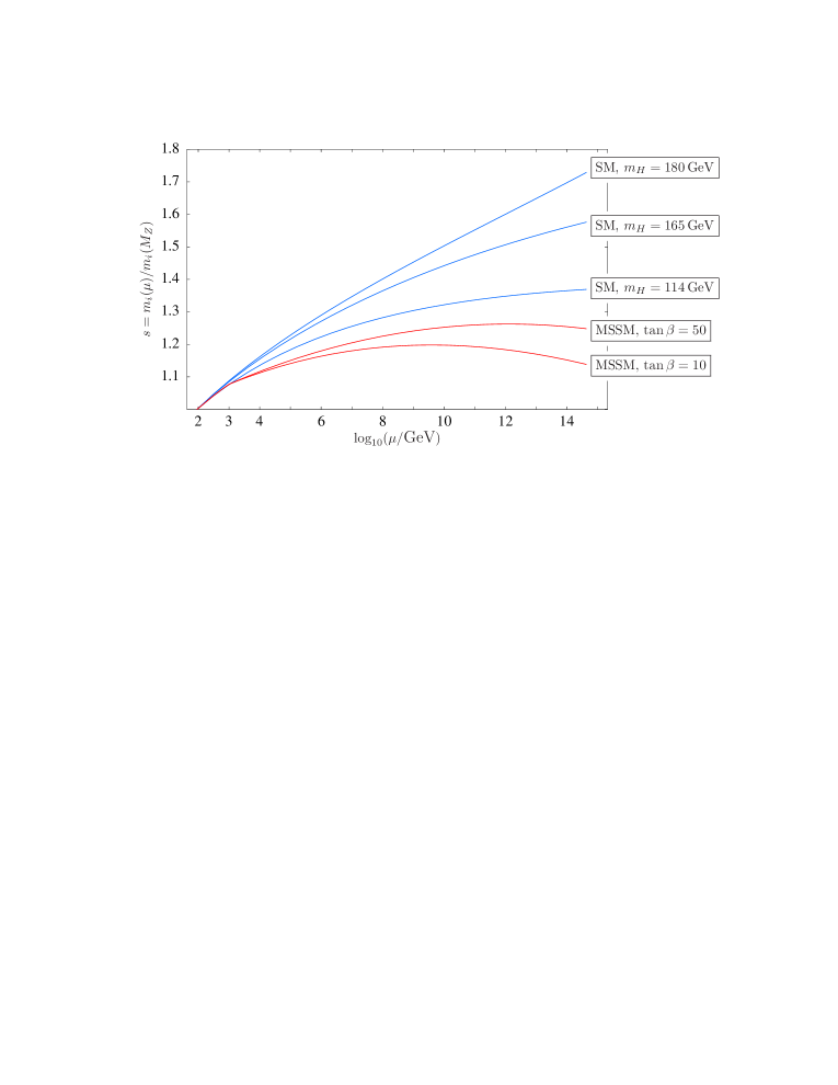
Figure 4: Scaling of the masses under the renormalization group in the SM and MSSM. The mixing parameters are chosen to be the LMA best-fit values (cf. Tab. 1), but they influence the running only marginally. We further used a SUSY-breaking scale $M_{\mathrm{SUSY}}=1\,\mathrm{TeV}$. The upper curves show the evolution in the SM for $m_{H}=114\,\mathrm{GeV}$, $m_{H}=165\,\mathrm{GeV}$ and $m_{H}=180\,\mathrm{GeV}$, the lower ones correspond to the MSSM for $\tan\beta=10$ and $\tan\beta=50$ with $m_{H}=120\,\mathrm{GeV}$. These plots apply for all mass eigenvalues, except for large $\tan\beta$ in the MSSM where the scaling of $m_{3}$ is shown (using zero phases). Note also that a different SUSY-breaking scale changes the scaling factor in the MSSM.

As already mentioned, substantial deviations from the common scaling arise in the MSSM for large $\tan\beta$. There is a plethora of effects which can be understood with the aid of (15) and (17). In order to give an interesting example, we show the evolution of the mass eigenvalues for $m_{\mathrm{min}}=0.19\,\mathrm{eV}$ (where $m_{\mathrm{min}}=\min\{m_{1},m_{2},m_{3}\}$) in the MSSM with $\tan\beta=50$ in Fig. 5. A particular interesting effect is that for an inverted mass spectrum the property $|\Delta m^{2}_{\mathrm{atm}}|>\Delta m^{2}_{\mathrm{sol}}$ possibly does not survive the RG evolution. In other words, what looks like a normal mass hierarchy at high energies turns out to become an inverted hierarchy at low energies (cf. Fig. 5(b)). From the dependence on the $y_{\tau}^{2}$ terms (cf. Eqs. (16) and (18)), we find that this effect can disappear if $\delta$ is large.

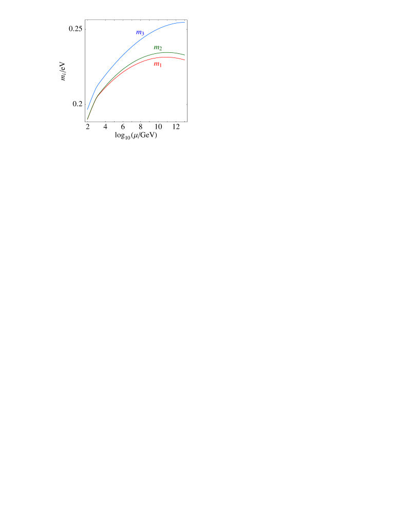
(a) Normal mass hierarchy

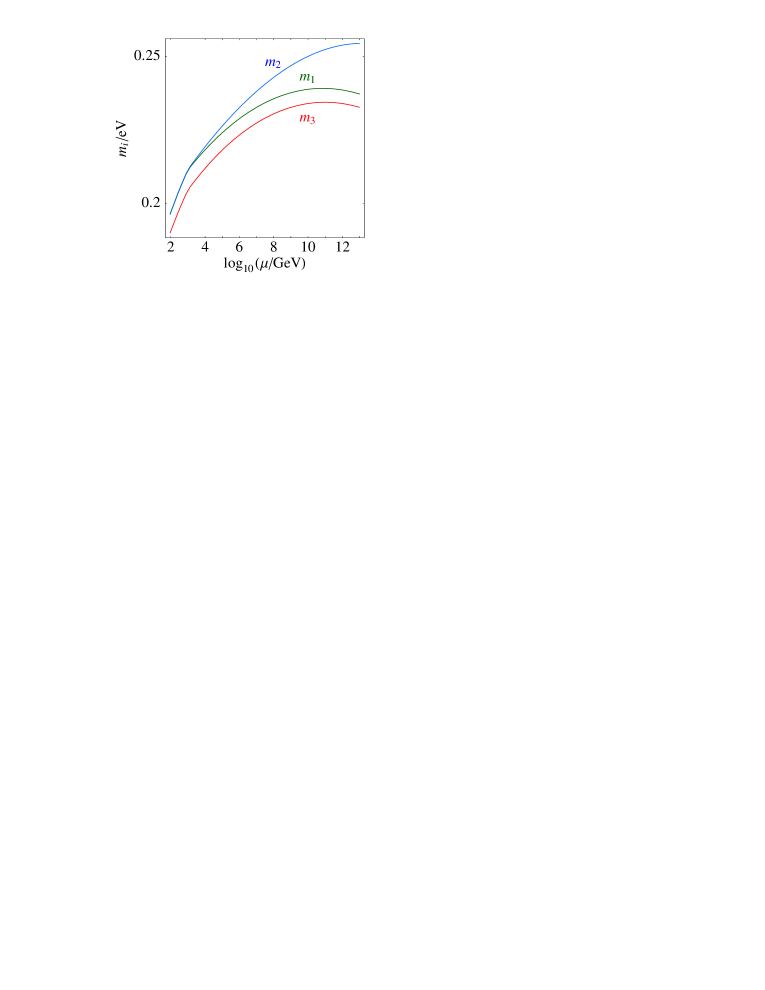
(b) Inverted mass hierarchy

Figure 5: Running of the light neutrino masses for a normal and an inverted mass hierarchy and $m_{\mathrm{min}}=0.19\,\mathrm{eV}$ in the MSSM with $\tan\beta=50$ and $M_{\mathrm{SUSY}}=1\,\mathrm{TeV}$. The mixing parameters are chosen to be the LMA best-fit values. The phases are zero in this example. In the inverted case, $\Delta m^{2}_{\mathrm{sol}}$ becomes greater than $|\Delta m^{2}_{\mathrm{atm}}|$.

2.3.5 RG Evolution of $\boldsymbol{\Delta m_{\mathrm{sol}}^{2}}$

The RGE for the solar mass squared difference is given in Eq. (17a). In the SM and the MSSM with small $\tan\beta$, the running is due to the common scaling of the masses described in the previous section and thus virtually independent of the mixing parameters. For large $\tan\beta$ and nearly degenerate masses, the influence of CP phases, in particular the Dirac phase, is crucial. The numerical example in Fig. 6 confirms this expectation and furthermore shows that $\Delta m_{\mathrm{sol}}^{2}$ runs dramatically. On the one hand, it can grow by more than an order of magnitude. As we have seen in Fig. 5, $\Delta m_{\mathrm{sol}}^{2}$ can even get larger than $|\Delta m_{\mathrm{atm}}^{2}|$. On the other hand, it can run to $0$ at energy scales slightly beyond the maximum of $10^{13}\,\mathrm{GeV}$ shown in the figure. For large $\tan\beta$, $\Delta m_{\mathrm{sol}}^{2}\ll m_{1}^{2}$ and not too small $\theta_{13}$, the first term in $F_{\mathrm{sol}}$ is essential for understanding these effects, since it is proportional to the sum of the masses squared rather than the difference. For $\delta=\pi$ and $\theta_{13}$ near the CHOOZ bound, its sign is negative and its absolute value maximal, which causes the evolution of $\Delta m_{\mathrm{sol}}^{2}$ towards zero. For $\delta=0$, the sign becomes positive, so that the running towards larger values is enhanced, which explains the upper boundary of the light-gray region in Fig. 6.

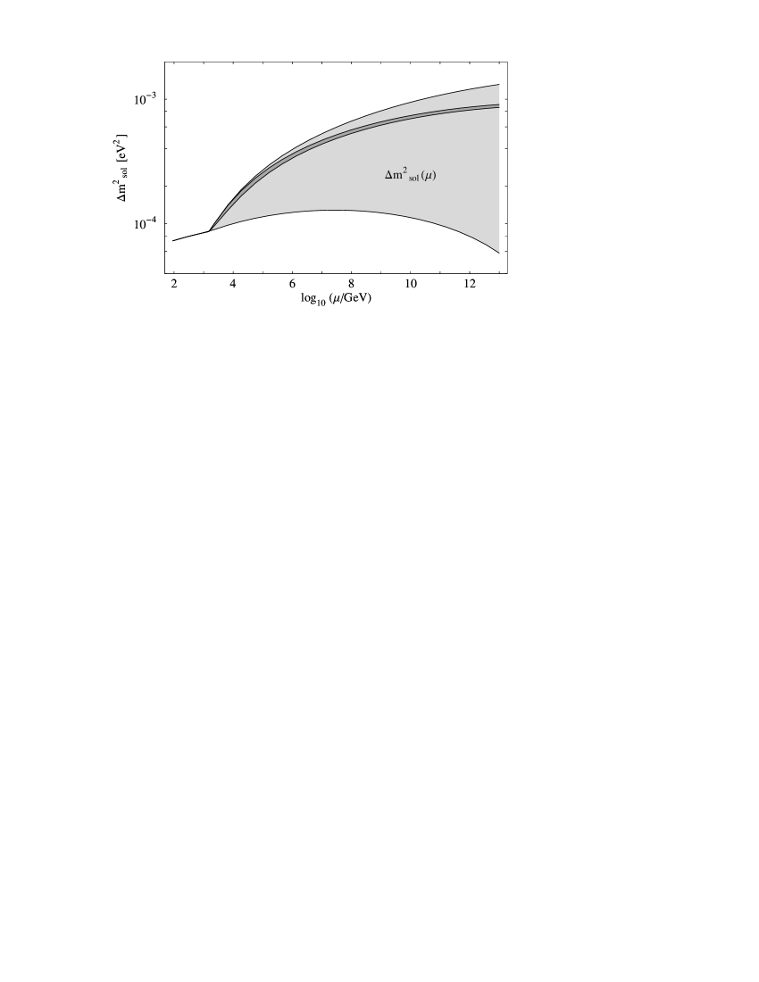
Figure 6: RG evolution of $\Delta m_{\mathrm{sol}}^{2}$ in the MSSM with $\tan\beta=50$, a normal mass hierarchy and $m_{1}=0.1\,\mathrm{eV}$. The dark-gray region shows the evolution with LMA best-fit values for the neutrino parameters, $\theta_{13}\in[0^{\circ},9^{\circ}]$ and all CP phases equal to zero. The light-gray regions show the evolution, which is possible, if arbitrary CP phases are allowed.

2.3.6 RG Evolution of $\boldsymbol{\Delta m_{\mathrm{atm}}^{2}}$

From the numerical example in Fig. 7, we see that $\Delta m_{\mathrm{atm}}^{2}$ can be damped by the phases, but not significantly enhanced. Depending on the CP phases, $\Delta m_{\mathrm{atm}}^{2}$ grows by about 50% – 95%. Analogously to above, the maximal damping is mainly due to the first term in $F_{\mathrm{atm}}$, so that it occurs for large $\theta_{13}$ and $\delta=0$. Compared to the case of the solar mass squared difference, the influence of $\delta$ is generically smaller here, because $\Delta m_{\mathrm{atm}}^{2}/m_{i}^{2}$ is larger and because the phase-independent terms in the RGE do not nearly cancel.

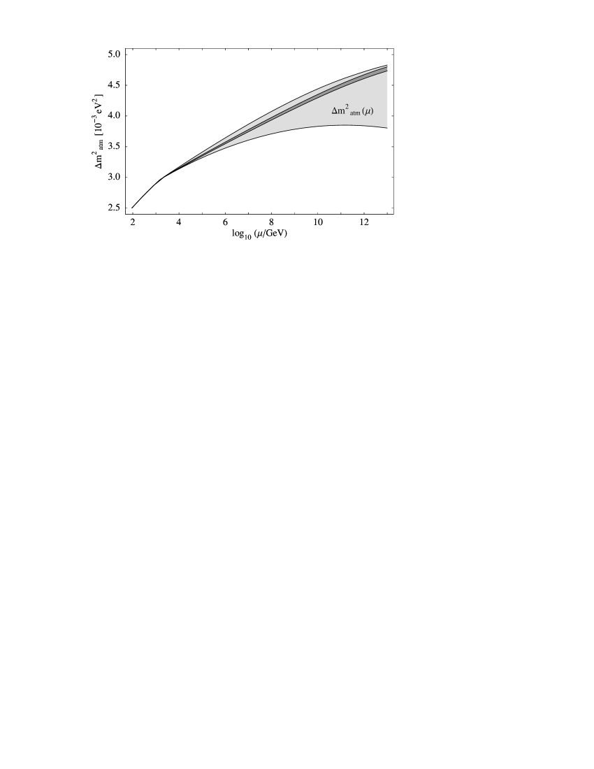
Figure 7: RG evolution of $\Delta m_{\mathrm{atm}}^{2}$ in the MSSM with the same input parameters as in Fig. 6.

2.4 RG Running of the Dirac and Majorana Phases

Most earlier studies of RG effects either neglected phases or concentrated on the special case of a Majorana parity, where one or both of the Majorana phases are $\pi$. We have seen that they can have a dramatic influence on the running of the masses and mixings. Moreover, many effects are affected by phases, e.g.  neutrinoless double beta decay, or require phases, e.g. leptogenesis.

Of course, if the phases are given at some scale, they also change due to the RG evolution. We now discuss the running of the phases themselves and give numerical examples. In general, a significant evolution of the phases is expected for nearly degenerate and inverted hierarchical mass patterns, since the RGEs (11)–(13) contain the ratios $m_{1}m_{2}/\Delta m^{2}_{\mathrm{sol}}$.

2.4.1 RG Evolution of the Dirac Phase

The running of the Dirac phase $\delta$ is given by Eq. (11) for $y_{e}=y_{\mu}=0$. An interesting possibility is the radiative generation of a Dirac phase by Majorana phases [11]: A non-zero $\delta$ is produced by RG effects, since some of the terms in the RGE (11) do not vanish for $\delta\rightarrow 0$. Fig. 8 shows an example. The most important term in this context is the first one in $\delta^{(0)}$. As it is proportional to $\sin(\varphi_{1}-\varphi_{2})$, the effect is suppressed for $\varphi_{1}=\varphi_{2}$. For small but non-zero values of $\theta_{13}$, the term involving $\delta^{(-1)}$ also contributes significantly because of the factor $\theta_{13}^{-1}$. For $\varphi_{1}=\varphi_{2}$, this contribution is suppressed as well, since the parts proportional to $m_{1}$ and $m_{2}$, respectively, nearly cancel.

Figure 8: Radiative generation of a Dirac phase in the MSSM with $\tan\beta=30$ and a normal hierarchy. Here the running is from high to low energy, i.e.  the boundary conditions are given at the see-saw scale. $\delta$ is zero there but large at $M_{Z}$. The other starting values are $\theta_{12}=18^{\circ}$, $\theta_{13}\in\{1^{\circ},3^{\circ},6^{\circ}\}$, $\theta_{23}=34^{\circ}$, $m_{1}=0.17\,\mathrm{eV}$, $\Delta m^{2}_{\mathrm{atm}}=3.8\cdot 10^{-3}\,\mathrm{eV}^{2}$, $\Delta m^{2}_{\mathrm{sol}}=5.7\cdot 10^{-4}\,\mathrm{eV}^{2}$, $\varphi_{1}=16^{\circ}$, $\varphi_{2}=140^{\circ}$.

In the case of an inverted hierarchy with $\tan\beta$ varying between 30 and 50, Dirac phases of about $15^{\circ}$ to $30^{\circ}$ can be generated. Now the term involving $\delta^{(-1)}$ receives an additional suppression from the small value of $m_{3}$, so that the subleading effects described above become unimportant. Hence, the running of $\delta$ is independent of $\theta_{13}$ and depends only on the difference of the Majorana phases to a very good approximation.

Before we turn to the evolution of the Majorana phases, let us discuss some further properties of the RGE for $\delta$ that are also valid beyond the special case of a radiative generation of this phase. To start with, the most important term in $\dot{\delta}$ depends only on the difference of the Majorana phases. Consequently, the evolution is expected to stay roughly the same if both phases change by the same value. A comparison with numerical results shows that this is true only to a first approximation. If one starts with $\varphi_{2}=0$ and increments it step by step, the running of $\delta$ is increasingly damped. The main reason for this is the second term in square brackets in $\delta^{(-1)}$ (the one proportional to $m_{2}$), whose sign is opposite to that of the leading term for $\delta<\varphi_{2}$. This term grows with $\varphi_{2}$, while the previous one (proportional to $m_{1}$) does not change much as long as $\varphi_{1}$ is close to $90^{\circ}$. The situation can be very different for smaller values of $\theta_{13}$. Now the initial rise of $\delta$ is enhanced, so that it can become larger than $\varphi_{2}$. Then the sign of the aforementioned second term in square brackets changes, so that it no longer damps the evolution but amplifies it.

With a strong normal hierarchy, RG effects are usually tiny. The running of the Dirac phase is one of the few examples where this is not always the case. Due to the terms proportional to $\theta_{13}^{-1}$ in the RGE, a significant evolution is possible for small $\theta_{13}$. However, one has to keep in mind that a measurement of $\delta$ is very hard in this case.

Regardless of the mass hierarchy, the limit $\theta_{13}\to 0$ is dangerous, because in this case the RGE (11) diverges. However, we can show that $\dot{\delta}$ remains well-defined: The derivative of the MNS matrix $U$ is given by (B.9), $\dot{U}=U\cdot T$, where $U$ and $T$ are continuous. Hence, $U_{13}(t)$ describes a continuously differentiable curve in the complex plane. Consequently, $\theta_{13}$ and $\delta$ are continuously differentiable even for $\theta_{13}=0$, if $\delta$ is extended continuously at this point. Note that restricting the parameters to certain ranges can nevertheless result in discontinuities. For example, if the RG evolution causes $\theta_{13}$ to change its sign and if we demand $0\leq\theta_{13}<\frac{\pi}{2}$, then there will be a kink in the evolution of $\theta_{13}$ and $\delta$ will jump by $\pi$. However, even in the presence of such artificial discontinuities there must still be finite one-sided limits for $\delta$ and $\dot{\delta}$ as $\theta_{13}$ approaches 0.

The limit for $\delta$ is determined by the requirement that $\dot{\delta}$ remains finite. Then the divergence of $\theta_{13}^{-1}$ has to be canceled by $\delta^{(-1)}$. For $\varphi_{1}=\varphi_{2}=0$, this obviously implies $\delta=0$ or $\delta=\pi$. In the general case, a short calculation yields

$$\cot\delta=\frac{m_{1}\cos\varphi_{1}-\left(1+\zeta\right)m_{2}\,\cos\varphi_{2}-\zeta m_{3}}{m_{1}\sin\varphi_{1}-\left(1+\zeta\right)m_{2}\,\sin\varphi_{2}}\;.$$ (25)

Due to the periodicity of $\cot$, there are two solutions differing by $\pi$, corresponding to the different limits on the two sides of a node of $\theta_{13}$.

2.4.2 RG Evolution of the Majorana Phases

While the RGEs for the Majorana phases are somewhat lengthy, there is a simple expression for the running of their difference for small $\theta_{13}$,

$$\dot{\varphi}_{1}-\dot{\varphi}_{2}=\frac{Cy_{\tau}^{2}}{4\pi^{2}}\,\frac{m_{1}m_{2}}{\Delta m^{2}_{\mathrm{sol}}}\,\cos 2\theta_{12}\,\sin^{2}\theta_{23}\,\sin(\varphi_{1}-\varphi_{2})+\mathscr{O}(\theta_{13})\;.$$ (26)

It shows that for $\theta_{13}=0$, the phases remain equal, if they are equal at some scale. Obviously, $\dot{\varphi}_{1}-\dot{\varphi}_{2}>0$ for $\varphi_{1}>\varphi_{2}$ and vice versa, which means that the difference between the phases tends to increase with increasing energy. In other words, a large difference at the see-saw scale becomes smaller at low energy. An example is shown in Fig. 9.

Figure 9: Running of the Majorana phases in the MSSM with a normal hierarchy, $\tan\beta=50$, $\varphi_{1}=75^{\circ}$, $\varphi_{2}=70^{\circ}$, $\theta_{13}=0$, $m_{1}=0.15\,\mathrm{eV}$, and LMA best-fit values for the mass squared differences, $\theta_{12}$ and $\theta_{23}$ at $M_{Z}$. RG effects are substantial, and the difference $\varphi_{1}-\varphi_{2}$ increases with increasing energy.

If $\varphi_{1}-\varphi_{2}$ is not too small, a non-zero $\theta_{13}$ tends to damp its running. This is due to a term in the RGE for $\varphi_{1}$ whose sign is opposite to that of the leading one in Eq. (26) and which is proportional to $\sin\theta_{13}\,\cot\theta_{12}$. This term can grow important if $\theta_{12}$ becomes small with increasing energy.

For $\varphi_{1}=\varphi_{2}$ the evolution of the Majorana phases is suppressed, since the leading terms in the RGEs (13) and (14) are zero then. However, for larger $\tan\beta$ RG effects are still important. Non-linear effects caused by the decrease of the solar and atmospheric mixing angles are essential here, as the initial slope of the curves is extremely small due to the suppression by $\sin\theta_{13}$ and $\cos 2\theta_{23}$. For $\theta_{13}=5^{\circ}$, the second line in the RGE and the terms proportional to $\sin\theta_{13}$ are about equally important for the running of $\varphi_{1}$. The evolution of $\varphi_{2}$ is virtually independent of $\theta_{13}$, since the respective terms are not multiplied by $\cot\theta_{12}$, which again can become large as the energy increases because of the diminishing $\theta_{12}$, but by $\tan\theta_{12}$, which remains smaller than 1.

In principle, it is also possible to generate Majorana phases radiatively, if the CP phase is non-zero. However, it follows from the discussion in the previous paragraph that this only happens via terms proportional to $\sin\theta_{13}$.

3 Some Applications

The discussed RG effects obviously have important implications whenever masses and mixings at different energy scales enter the analysis.

3.1 Relating the Leptogenesis Parameters to Observations

One of the most attractive mechanisms for explaining the observed baryon asymmetry of the universe, $\eta_{B}=(6.5^{+0.4}_{-0.8})\cdot 10^{-10}$ [47], is leptogenesis [5]. In this scenario, $\eta_{B}$ is generated by the out-of-equilibrium decay of the same heavy singlet neutrinos which are responsible for the suppression of light neutrino masses in the see-saw mechanism. The masses of the heavy neutrinos are typically assumed to be some orders of magnitude below the GUT scale.

Though the parameters entering the leptogenesis mechanism cannot be completely expressed in terms of low-energy neutrino mass parameters, it is possible to derive bounds on the neutrino mass scale from the requirement of a successful leptogenesis [48]. Since, as we demonstrated in Sec. 2.3.4, the neutrino masses experience corrections of about 20-25% in the MSSM or more than 60% in the SM, we expect the corrections for such bounds to be sizable.

The maximal baryon asymmetry generated in the thermal version of this scenario is given by [49, 50, 48]

$$\eta_{B}^{\mathrm{max}}\,\simeq\,0.96\cdot 10^{-2}\,\varepsilon_{1}^{\mathrm{max}}\,\kappa_{\mathrm{f}}\;.$$ (27)

$\kappa_{\mathrm{f}}$ is a dilution factor which can be computed from a set of coupled Boltzmann equations (see, e.g.  [51]). In [48], an analytic expression for the maximal relevant CP asymmetry was derived,

$$\varepsilon_{1}^{\mathrm{max}}(m_{1},m_{3},\widetilde{m}_{1})\,=\,\frac{3}{16\pi}\,\frac{M_{1}\,m_{3}}{(v/\sqrt{2})^{2}}\left[1-\frac{m_{1}}{m_{3}}\left(1+\frac{m_{3}^{2}-m_{1}^{2}}{\widetilde{m}_{1}^{2}}\right)^{1/2}\right],$$ (28)

which refines the older bound

$$\varepsilon_{1}^{\mathrm{max}}(m_{1},m_{3})\,=\,\frac{3}{16\pi}\frac{M_{1}}{(v/\sqrt{2})^{2}}\frac{\Delta m^{2}_{\mathrm{atm}}+\Delta m^{2}_{\mathrm{sol}}}{m_{3}}$$ (29)

and is valid for a normal mass hierarchy in the SM as well as in the MSSM. $\widetilde{m}_{1}$ is defined by

$$\widetilde{m}_{1}=\frac{(m_{\mathrm{D}}^{\dagger}m_{\mathrm{D}})_{11}}{M_{1}}$$ (30)

with $m_{\mathrm{D}}\sim Y_{\mathrm{\nu}}$ being the neutrino Dirac mass and typically lies between $m_{1}$ and $m_{3}$. It can be constrained by the requirement of successful leptogenesis because it controls the dilution of the generated asymmetry. The authors of [48] introduced the ‘neutrino mass window for baryogenesis’ which corresponds to the region in the $\widetilde{m}_{1}$-$M_{1}$ plane allowing for successful thermal leptogenesis. The shape and size of the ‘mass window’ depends on $\overline{m}=\sqrt{m_{1}^{2}+m_{2}^{2}+m_{3}^{2}}$, i.e. it becomes smaller for increasing $\overline{m}$, and $\overline{m}\geq 0.2\,\mathrm{eV}$ is not compatible with thermal leptogenesis.

The calculations relevant for leptogenesis, however, refer to processes at very high energies, and therefore the RG evolution of the input parameters has to be taken into account [52]. The correct procedure would be to assume specific values for the neutrino mass parameters at low energy, taking into account the experimental input, evolve them to the scale $M_{1}$ and test the leptogenesis mechanism using these values. As the full calculation is beyond the scope of this paper, we present the evolution of the relevant mass parameters, i.e.  the light neutrino masses, to the leptogenesis scale $M_{1}$ and estimate the size of the error arising if RG effects are neglected.

As discussed in Sec. 2.3.4, there are basically two cases which have to be distinguished, the case of the SM or the MSSM with small $\tan\beta$, and the case of the MSSM with large $\tan\beta$.

In the first case, running effects can be understood to arise due to the rescaling of the light neutrino mass eigenvalues under the renormalization group. From Eq. (29) it is clear that the maximal CP asymmetry scales like the masses. This statement also holds for the asymmetry from Eq. (28), if $\widetilde{m}_{1}$ is a linear combination of the light mass eigenvalues. Hence, the RG yields an enhancement of the CP asymmetry of between 10% and 80%, which can be read off from Fig. 4. These effects are almost completely independent of the low-energy CP phases. On the other hand, the dilution factor $\kappa_{\mathrm{f}}$ is expected to become tiny since larger mass eigenvalues imply larger Yukawa couplings, which makes the washout more efficient. This expectation is substantiated by the fact that $\overline{m}$, which controls an important class of washout processes, also increases under the renormalization group, i.e. it scales like the masses. As a detailed numerical calculation of the dilution factor is beyond the scope of this paper, we refer to [51], from which we see that in the region of interest, i.e.  the edge of the mass window, $\kappa_{\mathrm{f}}$ decreases exponentially. From this behavior, which is also in accordance with the analytic approximations (see, e.g.  [53, 54]), we expect that the neutrino mass window for baryogenesis will rather shrink than become larger when RG effects are properly taken into account.

In the second case, i.e.  in the MSSM for large $\tan\beta$, we distinguish between hierarchical and degenerate mass spectra. In the hierarchical spectrum, the running of $\varepsilon_{1}^{\mathrm{max}}$ is to a high accuracy given by the running of $m_{3}$, so that in this case Fig. 4 yields the relevant plot. The scaling depends on $\tan\beta$. In order to illustrate this dependence, we pick $M_{1}=10^{10}\,\mathrm{GeV}$ and plot $\overline{m}_{\mathrm{rel}}:=\overline{m}(10^{10}\,\mathrm{GeV})/\overline{m}(M_{Z})$ in Fig. 10(a) as a function of $\tan\beta$, including small values of this parameter as well. It is clear that $\overline{m}\approx m_{3}$ so that Fig. 10(a) also shows the scaling of $\varepsilon_{1}^{\mathrm{max}}$. Since $\tan\beta=10$ and $\tan\beta=50$ correspond to extreme cases, the scaling factor for different $M_{1}$ can be read off from Fig. 4 by interpolation.

In the case of a quasi-degenerate mass spectrum (and large $\tan\beta$), the CP asymmetry can run stronger than the average mass scale because, as we already have seen in Sec. 2.3.5 and 2.3.6, the mass squared differences can experience a stronger RG enhancement than the squares of the mass eigenvalues. We show the evolution of $\varepsilon_{\mathrm{rel}}:=\varepsilon_{1}^{\mathrm{max}}(10^{10}\,\mathrm{GeV})/\varepsilon_{1}^{\mathrm{max}}(M_{Z})$ in Fig. 10(b). To produce this plot, we employed (29) and inserted the running mass parameters. For this combination of parameters, the low-energy phases do influence the evolution of $\varepsilon_{\mathrm{rel}}$ by damping its running, and the plot shows the maximal evolution, which means that the phases are simply set to zero. The running effects are even larger for the new bound (28), since it is more sensitive to the mass splittings than the old one. More precisely, for highly degenerate mass spectra it is much smaller than the old one and the degeneracy can be lifted by running effects. This strong enhancement of the CP asymmetry may even overcompensate the decrease of the dilution factor for large $\tan\beta$, so that the parameter region compatible with thermal leptogenesis grows.

(a) $\tan\beta$-dependence of the scaling of $\overline{m}$.

(b) $m_{1}$-dependence of $\varepsilon_{\mathrm{rel}}$ for $\tan\beta=50$.

Figure 10: Radiative enhancement of $\overline{m}$ and the CP asymmetry in the MSSM. We show only the case of a normal mass hierarchy, since an inverted hierarchy yields virtually the same plot. We assume a SUSY-breaking scale $M_{\mathrm{SUSY}}=1\,\mathrm{TeV}$, a leptogenesis scale of $10^{10}\,\mathrm{GeV}$, and zero phases. The mixing angles and mass squared differences are the LMA best-fit values. We define $\varepsilon_{\mathrm{rel}}:=\varepsilon_{1}^{\mathrm{max}}(10^{10}\,\mathrm{GeV})/\varepsilon_{1}^{\mathrm{max}}(M_{Z})$. In the case of degenerate masses (see the right part of plot (b)), $\varepsilon_{1}^{\mathrm{max}}$ can run stronger than the mass eigenvalues since the mass squared differences can have a stronger dependence on the renormalization scale than the squares of the mass eigenvalues (cf. Fig. 5).

Altogether, we have presented the relevant mass parameters at the scale of leptogenesis, thus making it convenient to take into account RG effects in future studies. Moreover, we have estimated the impact of the renormalization effects, and found that there are two effects in opposite directions: The CP asymmetry is enhanced because the mass squared differences increase, and the dilution of the baryon asymmetry is more effective since the overall mass scale rises due to RG effects. As the dependence of the dilution factor on the mass scale is stronger than that of the CP asymmetry, we expect the mass window for baryogenesis to shrink when RG effects are included in the analysis. An exception is the case of large $\tan\beta$, where the situation is more complicated.

Note also that there exist different, non-thermal baryogenesis mechanisms [55] in which the masses of the light neutrinos may be almost degenerate [56]. In these kinds of scenarios, RG effects increase the baryon asymmetry, since $\varepsilon_{1}$ increases, while the effects from the expected decrease of the dilution factor do not occur.

3.2 RG Evolution of Bounds on the Neutrino Mass Scale

The absolute neutrino mass scale at low energy is restricted by low-energy experiments such as searches for $0\nu\beta\beta$ decay and cosmological observations. As usual, the RG evolution of the results has to be taken into account in order to translate the experimental results into constraints on high-energy theories.

3.2.1 Neutrinoless Double Beta Decay

The amplitude of $0\nu\beta\beta$ decay is proportional to the effective neutrino mass

$$\Braket{m_{\nu}} = (m_{\nu})_{11}\ =\ \Bigl{|}\sum_{i}U_{1i}^{2}\,m_{i}\Bigr{|}$$ (31)

$$= \left|m_{1}\,c_{12}^{2}c_{13}^{2}\,e^{\mathrm{i}\varphi_{1}}+m_{2}\,s_{12}^{2}c_{13}^{2}\,e^{\mathrm{i}\varphi_{2}}+m_{3}\,s_{13}^{2}\,e^{2\mathrm{i}\delta}\right|\;,$$

where $U$ is the MNS matrix. Instead of inserting the lengthy RGEs for all the quantities in the second line in order to calculate the RG evolution of $\Braket{m_{\nu}}$, it is much more convenient to use Eq. (3), which directly yields

$$16\pi^{2}\>\frac{\mathrm{d}}{\mathrm{d}t}\Braket{m_{\nu}}\,=\,\left(2C\,y_{e}^{2}+\alpha\right)\Braket{m_{\nu}}\;.$$ (32)

As the first term is negligible, the RG change of the effective neutrino mass is basically caused by the universal rescaling of the neutrino masses alone. It is completely independent of the other neutrino mass parameters, since neither the running of $y_{e}$ nor that of the terms in $\alpha$ is sensitive to them. Besides, the value of $\tan\beta$ is not very important here, because $y_{e}^{2}$ is always tiny and $\alpha$ contains only the up-type quark Yukawa couplings in the MSSM. However, there is a dependence on the Higgs mass in the SM.

Currently, the best experimental upper limit on the effective neutrino mass is about $\Braket{m_{\nu}}<0.35\,\mathrm{eV}$ [57, 58], with some uncertainty due to nuclear matrix elements. Fig. 11 shows the running of this limit in the SM and the MSSM. As it is very close to the best-fit value of the recently claimed evidence for double beta decay, $\Braket{m_{\nu}}=0.39\,\mathrm{eV}$ [59], the evolution of the latter is nearly identical. The SM plot contains three curves corresponding to different Higgs masses in the current experimentally allowed region. In the MSSM, the light Higgs mass is chosen to be about $120\,\mathrm{GeV}$. The running is much more significant in the SM than in the MSSM because of the contribution of the Higgs self-coupling.

(a) SM

(b) MSSM ($\tan\beta=50$, $M_{\mathrm{SUSY}}=1.5\,\mathrm{TeV}$)

Figure 11: Extrapolation of the experimental upper limit on the effective neutrino mass for $0\nu\beta\beta$ decay, $\langle m_{\nu}\rangle=0.35\,\mathrm{eV}$, to higher energies. The SM curves correspond to Higgs masses of $114\,\mathrm{GeV}$, $165\,\mathrm{GeV}$ and $190\,\mathrm{GeV}$ (from bottom to top). In the MSSM, a light Higgs mass of $120\,\mathrm{GeV}$ is used.

3.2.2 WMAP Bound

Combining the observations of the cosmic microwave background by the WMAP satellite with other astronomical data allows to place an upper bound of about $0.7\,\mathrm{eV}$ onto the sum of the light neutrino masses [47]. This implies

$$m_{i}\lesssim 0.23\,\text{eV}$$ (33)

for each mass eigenvalue. Analogous to the limit from $0\nu\beta\beta$ decay in the previous section, this bound is modified substantially by the RG evolution. This is shown in Fig. 12 for the eigenvalue $m_{3}$. As discussed in Sec. 2.3.4, the running of the mass eigenvalues is not sensitive to the mixing parameters in the SM, but it depends on the Higgs mass. In the MSSM, the variation of the phases causes a slight modification of the running, but its order of magnitude is only a few percent even for the large $\tan\beta$ used in the plot. The influence of $\theta_{13}$ is negligible. Interestingly, the evolution of the sum of the mass eigenvalues is virtually independent of the mixing parameters for nearly degenerate neutrinos both in the SM and in the MSSM. This can be explained by considering the sum of the RGEs (15). For $m_{1}\sim m_{2}\sim m_{3}$, the terms proportional to $y_{\tau}^{2}$ add up to 1, with small corrections of the order of $\frac{\Delta m^{2}_{\mathrm{atm}}}{m^{2}}$ and $\theta_{13}$.

(a) SM

(b) MSSM ($\tan\beta=50$, $M_{\mathrm{SUSY}}=1.5\mathrm{TeV}$)

Figure 12: Extrapolation of the upper limit on the neutrino mass from WMAP, $m_{i}\lesssim 0.23\,\mathrm{eV}$ to higher energies, represented by the running of the mass eigenvalue $m_{3}$. The SM curves correspond to Higgs masses of $114\,\mathrm{GeV}$, $165\,\mathrm{GeV}$ and $190\,\mathrm{GeV}$ (from bottom to top). In the MSSM, a light Higgs mass of $120\,\mathrm{GeV}$ is used.

3.3 Constraints on Neutrino Properties from RG Effects

One may wonder if deviations from $\theta_{13}=0$ and $\theta_{23}=\pi/4$ exist which are the consequence of radiative corrections. Let us assume therefore that $\theta_{13}=0$ or $\theta_{23}=\pi/4$ are given by some high-energy model. Low-energy deviations from the exact values are then RG effects, which can be compared to the sensitivities of future experiments. Therefore we investigate in a model-independent way the size of RG corrections to $\theta_{13}$ and $\theta_{23}$ from the running of the effective neutrino mass operator between the see-saw scale and the electroweak scale.

3.3.1 Corrections to $\boldsymbol{\theta_{13}}$

As pointed out in Sec. 2.3.2, it is a rather good approximation to assume $\dot{\theta}_{13}\simeq$ const. in Eq. (9), which leads to an RG evolution with a constant slope depending on the Dirac CP phase $\delta$ and the Majorana phases $\varphi_{1}$ and $\varphi_{2}$. Therefore, let us first apply the naive estimate (22) explicitly to the change of $\theta_{13}$ in the MSSM for nearly degenerate neutrinos. In this case, the enhancement factor $m^{2}/\Delta m^{2}_{\mathrm{atm}}$ leads to a generic change of $\theta_{13}$ under the RG that exceeds the detection limit of future experiments even for moderate values of $\tan\beta$. For example, $m_{1}=0.1\,\mathrm{eV}$ and $\tan\beta=30$ yield a change in $\sin^{2}2\theta_{13}$ of $\Delta\!\sin^{2}2\theta_{13}\sim 0.5\cdot 10^{-2}$, which is further enhanced by a factor of 4 if the Majorana phases are aligned properly.

In order to obtain a more detailed picture, we now apply Eq. (9) to calculate the RG correction to the initial value $\theta_{13}=0$ between some high energy scale $M_{1}$, where neutrino masses are generated, and low energy, i.e. $10^{2}\,\mathrm{GeV}$. In this case the initial value of the Dirac phase $\delta$ is determined by the analytic continuation Eq. (25). For the examples we take $M_{1}=10^{12}\,\mathrm{GeV}$. The approximate size of the RG corrections to $\sin^{2}2\theta_{13}$ in the MSSM is shown in Fig. 13. In the upper diagram it is plotted as a function of $\tan\beta$ and the lightest neutrino mass $m_{1}$ for constant Majorana phases $\varphi_{1}=0$ and $\varphi_{2}=\pi$. The lower diagram shows the dependence of the corrections on $\varphi_{1}$ and $\varphi_{2}$ for $\tan\beta=50$ and $m_{1}=0.08\,\mathrm{eV}$ in the case of a normal mass hierarchy. The diagrams look rather similar for an inverted hierarchy. Analytically, the pattern of the upper plot is easy to understand, and for the lower one there is a simple explanation as well. Consider partially or nearly degenerate neutrino masses. Then Eq. (9) yields to a reasonably good approximation

$$\dot{\theta}_{13} \approx \frac{Cy_{\tau}^{2}}{32\pi^{2}}\,\sin 2\theta_{12}\,\sin 2\theta_{23}\,\frac{m^{2}}{\Delta m^{2}_{\mathrm{atm}}}\left[\cos(\varphi_{1}-\delta)-\cos(\varphi_{2}-\delta)\right]$$ (34)

$$\propto \sin\frac{\varphi_{1}+\varphi_{2}-2\delta}{2}\,\sin\frac{\varphi_{1}-\varphi_{2}}{2}\;.$$

Applying an analogous approximation to Eq. (25), it can easily be shown that the first term in the second line is always $\pm 1$, so that the running is completely determined by the difference of the Majorana phases. This leads to the diagonal bands in Fig. 13, in particular the white one corresponding to $\varphi_{1}-\varphi_{2}=0$. If one starts with a small but non-zero $\theta_{13}$, which allows an arbitrary $\delta$, it turns out that the RG evolution quickly drives $\delta$ to a value satisfying Eq. (25), so that the final pattern of Fig. 13 is unchanged.

Planned reactor experiments [60] and next generation superbeam experiments [61, 62] are expected to have an approximate sensitivity on $\sin^{2}2\theta_{13}$ of $10^{-2}$. From Fig. 13 we find that the radiative corrections exceed this value for large regions of the currently allowed parameter space, unless there are cancellations due to Majorana phases, i.e. $\varphi_{1}\approx\varphi_{2}$ (which might be due to some symmetry). If so, the effects are generically smaller than $10^{-2}$ as can be seen from the lower diagram. Future upgraded superbeam experiments like JHF-HyperKamiokande have the potential to further push the sensitivity to about $10^{-3}$ and with a neutrino factory even about $10^{-4}$ might be reached.

From the theoretical point of view, one would expect that even if some model predicted $\theta_{13}=0$ at the energy scale of neutrino mass generation, RG effects would at least produce a non-zero value of the order shown in Fig. 13. Consequently, experiments with such a sensitivity have a large discovery potential for $\theta_{13}$. We should point out that this is a conservative estimate, since if neutrino masses are e.g. determined by GUT scale physics, model-dependent radiative corrections in the region between $M_{1}$ and $M_{\mathrm{GUT}}$ contribute as well [8, 9, 63, 64, 65, 66] and there can be additional corrections from physics above the GUT scale [67]. On the other hand, if experiments do not measure $\theta_{13}$, this will improve the upper bound on $\theta_{13}$. Parameter space regions where the corrections are larger than this bound will then appear unnatural from the theoretical side.

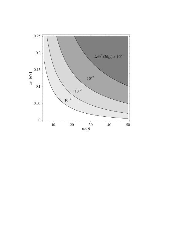
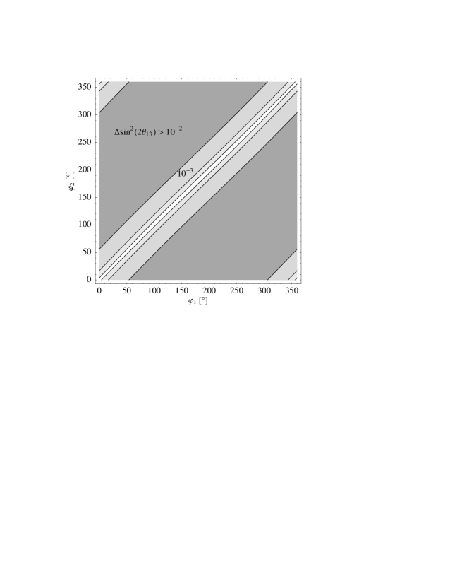
Figure 13: Corrections to $\theta_{13}$ from the RG evolution between $10^{2}$ and $10^{12}\,\mathrm{GeV}$ in the MSSM, calculated using the analytical approximations with initial conditions $\theta_{13}=0$ and LMA best-fit values for the remaining parameters. The upper diagram shows the dependence on $\tan\beta$ and on the mass of the lightest neutrino for the case of a normal mass hierarchy and phases $\varphi_{1}=0$ and $\varphi_{2}=\pi$. In the lower diagram the dependence on the Majorana phases $\varphi_{1}$ and $\varphi_{2}$ is shown for $\tan\beta=50$ and $m_{1}=0.08\,\mathrm{eV}$. The contour lines are defined as in the upper diagram. In order to apply Eq. (9) to the case $\theta_{13}=0$, where $\delta$ is undefined, the analytic continuation of Eq. (25) has been used.

3.3.2 Corrections to $\boldsymbol{\theta_{23}}$

We now consider the RG corrections which induce a deviation of $\theta_{23}$ from $\pi/4$, even if some model predicted this specific value at high energy. We apply the analytical formula (10) with a constant right-hand side in order to calculate the running in the MSSM between $M_{Z}$ and the see-saw scale, which we take as $M_{1}=10^{12}\,\mathrm{GeV}$ for our examples. As initial conditions we assume small $\theta_{13}$ at $M_{1}$ and low-energy best-fit values for the remaining lepton mixings and the neutrino mass squared differences. In leading order in $\theta_{13}$, the evolution is of course independent of the Dirac phase $\delta$.

The size of the RG corrections in the MSSM is shown in Fig. 14. From the upper diagram it can be read off for desired values of $\tan\beta$ and the lightest mass eigenvalue $m_{1}$ in an example with vanishing Majorana phases. The lower diagram shows its dependence on the Majorana phases $\varphi_{1}$ and $\varphi_{2}$ for $\tan\beta=50$, $m_{1}=0.1\,\mathrm{eV}$ and a normal mass hierarchy. The diagrams look rather similar in the case of an inverted hierarchy. The effects of the Majorana phases can easily be understood from Eq. (10). In the region with $\varphi_{1}\approx\varphi_{2}\approx\pi$ (again, this might be, e.g., due to some symmetry), both $|m_{2}\,e^{\mathrm{i}\varphi_{2}}+m_{3}|^{2}$ and $|m_{1}\,e^{\mathrm{i}\varphi_{1}}+m_{3}|^{2}$ are small for quasi-degenerate neutrinos, which gives the ellipse with small radiative corrections in the center of the lower diagram. Such cancellations are not possible with hierarchical masses, but the RG effects are generally not very large in this case, as shown by the upper plot.

Even if a model predicted $\theta_{23}=\pi/4$ at some high energy scale, we would thus expect radiative corrections to produce at least a deviation from this value of the size shown in Fig. 14, so that experiments with such a sensitivity are expected to measure a deviation of $\theta_{23}$ from $\pi/4$. The sensitivity to $\sin^{2}2\theta_{23}$ of future superbeam experiments like JHF-SuperKamiokande is expected to be approximately 1% (see e.g. [68]). This can now be compared with Fig. 14. We find that the radiative corrections exceed this value for large regions of the currently allowed parameter space, where no significant cancellations due to Majorana phases occur. This means that $\varphi_{1}$ and $\varphi_{2}$ must not be too close to $\pi$. Otherwise, the effects are generically smaller as can be seen from the lower diagram. Upgraded superbeam experiments or a neutrino factory might even reach a sensitivity of about $0.5$%. As argued for the case of $\theta_{13}$, if experiments measure $\theta_{23}$ rather close to $\pi/4$, parameter combinations implying larger radiative corrections than the measured deviation will appear unnatural from the theoretical point of view.

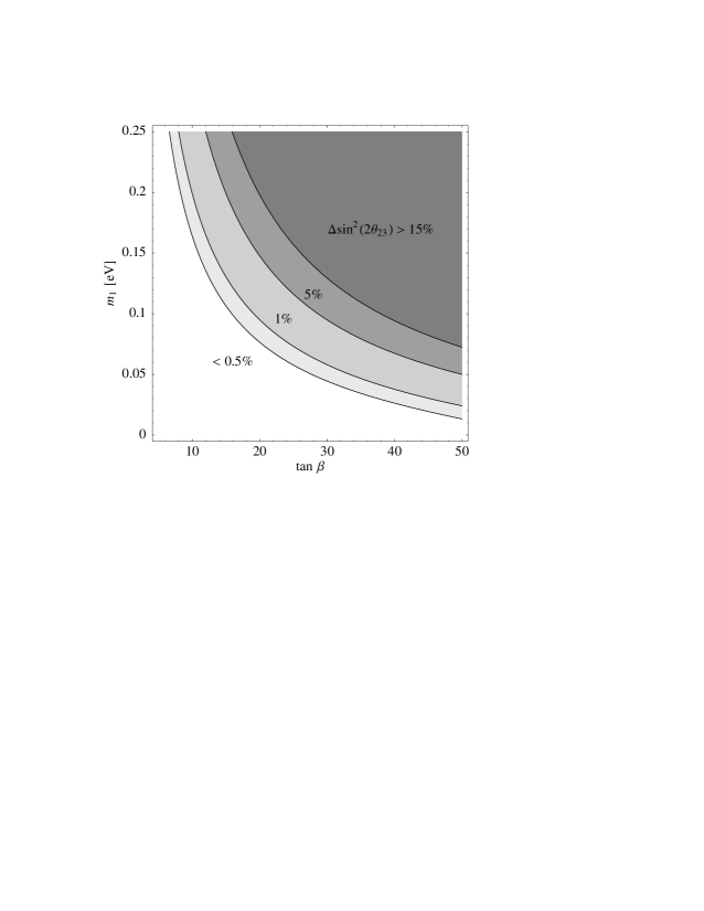
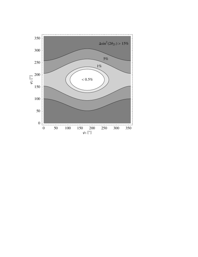
Figure 14: Corrections to $\theta_{23}$ from the RG evolution between $10^{2}\,\mathrm{GeV}$ and $10^{12}\,\mathrm{GeV}$ in the MSSM, calculated from the analytical approximation Eq. (10) with initial conditions $\theta_{23}=\pi/4$, small $\theta_{13}=0$ and LMA best-fit values for the remaining parameters. The upper diagram shows the dependence on $\tan\beta$ and on the mass $m_{1}$ of the lightest neutrino for the case of a normal mass hierarchy and phases $\varphi_{1}=\varphi_{2}=0$. In the lower diagram the dependence on the Majorana phases $\varphi_{1}$ and $\varphi_{1}$ is shown for the example $\tan\beta=50$ and $m_{1}=0.1$. Note that for small $\theta_{13}$ the results are independent of the Dirac phase to a good approximation.

4 Conclusions

We have derived compact expressions which allow an analytical understanding of the running of neutrino masses, leptonic mixing angles and CP phases in the SM and MSSM. The results are given directly in terms of these quantities as well as gauge and Yukawa couplings, and especially for a small angle $\theta_{13}$ the expressions become very simple, even when non-vanishing CP phases are present. We have extensively compared those formulae to numerical results and we have found that the RG evolution of the physical parameters is described qualitatively, and to a reasonable accuracy also quantitatively, very well. We have shown that Dirac and Majorana CP phases can have a drastic influence on the RG evolution of the mixing parameters. We have reproduced and illustrated some effects that were previously described in the literature. As a particularly interesting example, we have discussed the radiative generation of the Dirac phase from the Majorana phases. Besides, we have derived new results, for example concerning the running of the CP phases. Even though the RG effects for the mixing parameters in the SM are rather small, the RG effects for the masses are not, and have to be taken into account in any careful analysis which relates high and low energy scales. In the MSSM, especially for large $\tan\beta$, the evolution of the mixings and phases can be large.

The RG evolution has interesting phenomenological implications. In the case of leptogenesis, we have estimated the corrections which arise if the running is appropriately taken into account and found that the mass window for baryogenesis is likely to shrink when those corrections are considered. In order to simplify the inclusion of RG effects in future calculations, we provide the relevant information of the mass parameters at the leptogenesis scale. Furthermore, we investigated the extrapolation of the upper bounds on the neutrino mass scale from $0\nu\beta\beta$ decay experiments and WMAP to higher energy scales, where they become restrictions for model building. Experimentally one finds $\theta_{23}\simeq\pi/4$, $\theta_{13}\simeq 0$. The deviations from $\pi/4$ and zero may have a radiative origin and we calculated therefore in a model-independent analysis the RG corrections to $\theta_{23}=\pi/4$, $\theta_{13}=0$. With future precision experiments this may lead to interesting insights into model parameters.

To conclude, we have obtained analytic formulae which are a useful tool to understand the RG corrections, relevant whenever parameters at two different energy scales are compared. This has been demonstrated in the phenomenological applications.

Appendix

Appendix A Definition and Extraction of Mixing Parameters

A.1 Standard Parametrization

In this section we describe our conventions and how mixing angles and phases can be extracted from mass matrices. For a general unitary matrix we choose the so-called standard-parametrization

$$U = \operatorname{diag}(e^{\mathrm{i}\delta_{e}},e^{\mathrm{i}\delta_{\mu}},e^{\mathrm{i}\delta_{\tau}})\cdot V\cdot\operatorname{diag}(e^{-\mathrm{i}\varphi_{1}/2},e^{-\mathrm{i}\varphi_{2}/2},1)$$ (A.1)

where

$$V=\left(\begin{array}[]{ccc}c_{12}c_{13}&s_{12}c_{13}&s_{13}e^{-\mathrm{i}\delta}\\ -c_{23}s_{12}-s_{23}s_{13}c_{12}e^{\mathrm{i}\delta}&c_{23}c_{12}-s_{23}s_{13}s_{12}e^{\mathrm{i}\delta}&s_{23}c_{13}\\ s_{23}s_{12}-c_{23}s_{13}c_{12}e^{\mathrm{i}\delta}&-s_{23}c_{12}-c_{23}s_{13}s_{12}e^{\mathrm{i}\delta}&c_{23}c_{13}\end{array}\right)$$ (A.2)

with $c_{ij}$ and $s_{ij}$ defined as $\cos\theta_{ij}$ and $\sin\theta_{ij}$, respectively.

A.2 Extracting Mixing Angles and Phases

In this standard-parametrization, the mixing angles $\theta_{13}$ and $\theta_{23}$ can be chosen to lie between $0$ and $\frac{\pi}{2}$, and by reordering the masses, $\theta_{12}$ can be restricted to $0\leq\theta_{12}\leq\frac{\pi}{4}$. For the phases the range between $0$ and $2\pi$ is required. In order to read off the mixing parameters, we use the following procedure:

1. $\theta_{13}=\arcsin(|U_{13}|)$.

2. $\displaystyle\theta_{12}=\left\{\begin{array}[]{ll}\displaystyle\arctan\left(\frac{|U_{12}|}{|U_{11}|}\right)&\text{if}\;U_{11}\neq 0\\ \frac{\pi}{2}&\text{else}\end{array}\right.$

3. $\displaystyle\theta_{23}=\left\{\begin{array}[]{ll}\displaystyle\arctan\left(\frac{|U_{23}|}{|U_{33}|}\right)&\text{if}\;U_{33}\neq 0\\ \frac{\pi}{2}&\text{else}\end{array}\right.$

4. $\delta_{\mu}=\arg(U_{23})$

5. $\delta_{\tau}=\arg(U_{33})$

6. $\displaystyle\delta=-\arg\left(\frac{\displaystyle\frac{U_{ii}^{*}U_{ij}U_{ji}U_{jj}^{*}}{c_{12}\,c_{13}^{2}\,c_{23}\,s_{13}}+c_{12}\,c_{23}\,s_{13}}{s_{12}\,s_{23}}\right)$
   where $i,j\in\{1,2,3\}$ and $i\neq j$.

7. $\delta_{e}=\arg(e^{\mathrm{i}\delta}\,U_{13})$

8. $\displaystyle\varphi_{1}=2\arg(e^{\mathrm{i}\delta_{e}}\,U_{11}^{*})$

9. $\displaystyle\varphi_{2}=2\arg(e^{\mathrm{i}\delta_{e}}\,U_{12}^{*})$

Here we used the relation

$$U_{ii}^{*}U_{ij}U_{ji}U_{jj}^{*} = c_{12}\,c_{13}^{2}\,c_{23}\,s_{13}\left(e^{-\mathrm{i}\delta}\,s_{12}\,s_{23}-c_{12}\,c_{23}\,s_{13}\right)\;,$$

which holds for $i,j\in\{1,2,3\}$ and $i\neq j$. Note that this relation is often used in order to introduce the Jarlskog invariants [69]

$$J_{\mathrm{CP}} = \frac{1}{2}\left|\operatorname{Im}(U_{11}^{*}U_{12}U_{21}U_{22}^{*})\right|\,=\,\frac{1}{2}\left|\operatorname{Im}(U_{11}^{*}U_{13}U_{31}U_{33}^{*})\right|$$ (A.3)

$$= \frac{1}{2}\left|\operatorname{Im}(U_{22}^{*}U_{23}U_{32}U_{33}^{*})\right|\,=\,\frac{1}{2}\left|c_{12}\,c_{13}^{2}\,c_{23}\,\sin\delta\,s_{12}\,s_{13}\,s_{23}\right|\;.$$

For the sake of a better numerical stability, one can choose any of the three combinations. In particular, if the modulus of one of the $U_{ij}$ is very small, it turns out to be more accurate to choose a combination in which this specific $U_{ij}$ does not appear.

A.3 Leptonic Mixing Matrix

Since the effective neutrino mass matrix is symmetric, it can be diagonalized by a unitary matrix $U_{\nu}$,

$$U_{\nu}^{T}\,m_{\nu}\,U_{\nu}\,=\,\operatorname{diag}(m_{1},m_{2},m_{3})\;.$$ (A.4)

The form of $U$ depends on a prescription how to order the mass eigenvalues. In order to obtain a mixing matrix which can be compared with the experimental data, the choice of the prescription is somewhat subtle. From experiment we know that there is a small mass difference, called $\Delta m^{2}_{\mathrm{sol}}=m_{i}^{2}-m_{j}^{2}$, and a larger one, referred to as $\Delta m^{2}_{\mathrm{atm}}=m_{k}^{2}-m_{\ell}^{2}$. By convention, the masses are labeled such that $i,j\neq 3$ while either $k$ or $\ell$ equals 3. The different schemes are depicted in Fig. 15.

$\begin{array}[]{c}\vbox{\hbox{\includegraphics[scale={1}]{NormalHierarchy.eps}}}\\[28.45274pt] \phantom{\text{M\"{u}mmel}}\end{array}$

(a) Normal mass hierarchy.

$\begin{array}[]{c}\vbox{\hbox{\includegraphics[scale={1}]{InvertedHierarchy.eps}}}\\[28.45274pt] \phantom{\text{M\"{u}mmel}}\end{array}$

(b) Inverted mass hierarchy.

Figure 15: The normal and inverted mass hierarchy.

The mass label 2 is attached to the eigenvector with the lower modulus of the first component. We are doing this since we want to read off a mixing angle $\theta_{12}$ less then $45^{\circ}$.

The neutrino mixing matrix $U_{\mathrm{MNS}}$ can then be read off in the following way:

1. Diagonalize $Y_{e}^{\dagger}Y_{e}$ by $U_{e}$, i.e. $Y_{e}\to U_{e}^{\dagger}\cdot Y_{e}^{\dagger}\cdot Y_{e}\cdot U_{e}=\operatorname{diag}\left(y_{e}^{2},y_{\mu}^{2},y_{\tau}^{2}\right)$ where $y_{f}^{2}$ are positive for $f\in\{e,\mu,\tau\}$.

2. Change the basis according to $m_{\nu}\to m_{\nu}^{\prime}=U_{e}^{T}\cdot m_{\nu}\cdot U_{e}$.

3. Diagonalize $m_{\nu}^{\prime}$: $m_{\nu}^{\prime}\to U_{\mathrm{MNS}}^{T}\cdot m_{\nu}^{\prime}\cdot U_{\mathrm{MNS}}=\operatorname{diag}(m_{1},m_{2},m_{3})$ where $m_{i}>0$.

Then $U_{\mathrm{MNS}}$ contains the leptonic mixing angles which can be read off as described in Sec. A.2. Note that $m_{1}<m_{2}<m_{3}$ is not necessarily fulfilled, as we already mentioned before (cf. Fig. 15).

Appendix B Derivation of the Analytical Formulae

To derive the RGEs for the mixing parameters, we follow in general the methods of [70]. The RGE for $\kappa$ reads

$$16\pi^{2}\,\frac{\mathrm{d}\kappa}{\mathrm{d}t}\,=\,\alpha\,\kappa+P^{T}\,\kappa+\kappa\,P\;,$$ (B.5)

where all terms with trivial flavour structure are absorbed in $\alpha$. $\kappa$ can be diagonalized (in the basis where $Y_{e}$ is diagonal) by a unitary transformation,

$$U(t)^{T}\,\kappa(t)\,U(t)\,=\,D(t)\,=\,\frac{4}{v^{2}}\,\operatorname{diag}\big{(}m_{1}(t),m_{2}(t),m_{3}(t)\big{)}\;.$$ (B.6)

We hence obtain

$$\frac{\mathrm{d}}{\mathrm{d}t}\left(U^{*}\,D\,U^{\dagger}\right)=\dot{U}^{*}\,D\,U^{\dagger}+U^{*}\,D\,\dot{U}^{\dagger}+U^{*}\,\dot{D}\,U^{\dagger}$$ (B.7)

$$\stackrel{{\scriptstyle\eqref{eq:GeneralRGEforKappa}}}{{=}} \frac{1}{16\pi^{2}}\,\left(\alpha\,U^{*}\,D\,U^{\dagger}+P^{T}\,U^{*}\,D\,U^{\dagger}+U^{*}\,D\,U^{\dagger}\,P\right)\;.$$

Multiplying with $U^{T}$ from the left and with $U$ from the right yields

$$U^{T}\,\dot{U}^{*}\,D+D\,\dot{U}^{\dagger}\,U+\dot{D}\,=\,\frac{1}{16\pi^{2}}\left[\alpha\,D+P^{\prime\,T}\,D+D\,P^{\prime}\right]\;,$$ (B.8)

where we have introduced $P^{\prime}=U^{\dagger}\,P\,U$. The next step is defining an anti-Hermitian matrix $T$ by

$$\frac{\mathrm{d}}{\mathrm{d}t}U\,=\,U\,T\;.$$ (B.9)

With this definition, we find

$$\dot{D}\,=\,\frac{1}{16\pi^{2}}\,\left(\alpha\,D+P^{\prime\,T}\,D+D\,P^{\prime}\right)-T^{*}\,D+D\,T\;,$$ (B.10)

where the anti-hermiticity of $T$ was used. Since the left-hand side of this equation is diagonal and real per definition, the right-hand side has to possess these properties as well,

$$\dot{m}_{i}\,=\,\frac{1}{16\pi^{2}}\,\left(\alpha\,m_{i}+2\,P^{\prime}_{ii}\,m_{i}\right)+(T_{ii}-T_{ii}^{*})\,m_{i}\;.$$ (B.11)

Note that here and in the following equations, no sum over repeated indices is implied. The second bracket is purely imaginary, hence it has to cancel with the imaginary part of the first one,

$$2\,\operatorname{Im}T_{ii}\,=\,\frac{-1}{16\pi^{2}}\,(\operatorname{Im}\alpha+2\operatorname{Im}P^{\prime}_{ii})\;,$$ (B.12)

and we further confirm eq. (15) of [11], which translates with our conventions to

$$16\pi^{2}\,\dot{m}_{i}\,=\,\left(\operatorname{Re}\alpha+2\,\operatorname{Re}P^{\prime}_{ii}\right)\,m_{i}\;.$$ (B.13)

Eq. (B.12) differs from Eq. (19) of [11], where the imaginary part of $\alpha$ is not present; however, this difference is irrelevant in the SM and the MSSM, where $\alpha$ is real. By comparing the off-diagonal parts of (B.10) we find

$$m_{i}\,T_{ij}-T_{ij}^{*}\,m_{j}\,=\,-\frac{1}{16\pi^{2}}\,\left(P^{\prime\,T}_{ij}\,m_{j}+m_{i}\,P^{\prime}_{ij}\right)\;.$$ (B.14)

Adding and subtracting this equation and its complex conjugate, we obtain for $i\neq j$

$$16\pi^{2}\,\operatorname{Re}T_{ij} = -\frac{m_{j}\,\operatorname{Re}P^{\prime}_{ji}+m_{i}\,\operatorname{Re}P^{\prime}_{ij}}{m_{i}-m_{j}}\;,$$ (B.15a)

$$16\pi^{2}\,\operatorname{Im}T_{ij} = -\frac{m_{j}\,\operatorname{Im}P^{\prime}_{ji}+m_{i}\,\operatorname{Im}P^{\prime}_{ij}}{m_{i}+m_{j}}\;.$$ (B.15b)

Let us now focus on Hermitian $P$, which implies Hermitian $P^{\prime}$, for a moment. Using $\operatorname{Re}P^{\prime}_{ji}=\operatorname{Re}P^{\prime\,*}_{ij}=\operatorname{Re}P^{\prime}_{ij}$ and an analogous relation for $\operatorname{Im}P^{\prime}_{ij}$, we obtain in this case

$$16\pi^{2}\,\operatorname{Im}T_{ij} = -\frac{m_{i}-m_{j}}{m_{i}+m_{j}}\,\operatorname{Im}P^{\prime}_{ij}\;,$$ (B.16a)

$$16\pi^{2}\,\operatorname{Re}T_{ij} = -\frac{m_{i}+m_{j}}{m_{i}-m_{j}}\,\operatorname{Re}P^{\prime}_{ij}\;.$$ (B.16b)

In order to obtain the renormalization group equations for the mixing angles, we use (B.9),

$$U^{\dagger}\,\dot{U}=T\;.$$ (B.17)

Inserting the standard parametrization (A.1), we can express the left-hand side of (B.17) in terms of the mixing parameters and their derivatives. Now we can solve for the derivatives of the mixing parameters. Note that due to the separation of the evolution of the mass eigenvalues in equation (B.13), we have reduced the number of parameters from 12 to 9. The discussion so far has been very similar to the one of [11]. There, the RG evolution of the mixing parameters is expressed in terms of the mixing matrix elements and $P^{\prime}$.

In order to obtain rather short and more explicit formulae, which are e.g. useful for deriving the approximations of Sec. 2.1, we now consider (B.17) and label the mixing parameters as

$$\{\xi_{k}\}=\{\theta_{12},\theta_{13},\theta_{23},\delta,\delta_{e},\delta_{\mu},\delta_{\tau},\varphi_{1},\varphi_{2}\}\;.$$ (B.18)

We observe that the left-hand side of (B.17) is linear in $\dot{\xi}_{k}$. Therefore, by solving the corresponding system of linear equations, we can express the derivatives of the mixing parameters by the mixing parameters, the mass eigenvalues and the Yukawa couplings. The resulting formulae are still too long to be presented here but can be obtained from the web page http://www.ph.tum.de/~mratz/AnalyticFormulae/.

Finally, let us record that only the moduli of $U_{ij}$ enter into the diagonal elements of $P^{\prime}$, if $P$ is diagonal, $P=\operatorname{diag}(P_{1},P_{2},P_{3})$ (which is the case in the SM and MSSM in the basis we have used in the main part), since

$$P_{ii}^{\prime}=\sum_{jk}(U^{\dagger})_{ij}P_{jk}U_{ki}=\sum_{jk}U^{*}_{ji}P_{j}\delta_{jk}U_{ki}=\sum_{j}|U_{ji}|^{2}P_{j}\;.$$ (B.19)

Consequently, the evolution of the mass eigenvalues does not directly depend on the Majorana phases, as claimed in Sec. 2.3.4.

References

- [1] T. Yanagida, in Proceedings of the Workshop on the Unified Theory and the Baryon Number in the Universe (O. Sawada and A. Sugamoto, eds.), KEK, Tsukuba, Japan, 1979, p. 95.
- [2] S. L. Glashow, The future of elementary particle physics, in Proceedings of the 1979 Cargèse Summer Institute on Quarks and Leptons (M. Lévy et al., eds.), Plenum Press, New York, 1980, pp. 687–713.
- [3] M. Gell-Mann, P. Ramond, and R. Slansky, Complex spinors and unified theories, in Supergravity (P. van Nieuwenhuizen and D. Z. Freedman, eds.), North Holland, Amsterdam, 1979, p. 315.
- [4] R. N. Mohapatra and G. Senjanović, Neutrino mass and spontaneous parity violation, Phys. Rev. Lett. 44 (1980), 912.
- [5] M. Fukugita and T. Yanagida, Baryogenesis without grand unification, Phys. Lett. 174B (1986), 45.
- [6] M. Tanimoto, Renormalization effect on large neutrino flavor mixing in the minimal supersymmetric standard model, Phys. Lett. B360 (1995), 41–46, hep-ph/9508247.
- [7] J. R. Ellis and S. Lola, Can neutrinos be degenerate in mass?, Phys. Lett. B458 (1999), 310–321, hep-ph/9904279.
- [8] J. A. Casas, J. R. Espinosa, A. Ibarra, and I. Navarro, Naturalness of nearly degenerate neutrinos, Nucl. Phys. B556 (1999), 3–22, hep-ph/9904395.
- [9] J. A. Casas, J. R. Espinosa, A. Ibarra, and I. Navarro, Nearly degenerate neutrinos, supersymmetry and radiative corrections, Nucl. Phys. B569 (2000), 82–106, hep-ph/9905381.
- [10] P. H. Chankowski, W. Krolikowski, and S. Pokorski, Fixed points in the evolution of neutrino mixings, Phys. Lett. B473 (2000), 109, hep-ph/9910231.
- [11] J. A. Casas, J. R. Espinosa, A. Ibarra, and I. Navarro, General RG Equations for Physical Neutrino Parameters and their Phenomenological Implications, Nucl. Phys. B573 (2000), 652, hep-ph/9910420.
- [12] K. R. S. Balaji, A. S. Dighe, R. N. Mohapatra, and M. K. Parida, Radiative magnification of neutrino mixings and a natural explanation of the neutrino anomalies, Phys. Lett. B481 (2000), 33–38, hep-ph/0002177.
- [13] N. Haba, Y. Matsui, and N. Okamura, The effects of Majorana phases in three-generation neutrinos, Eur. Phys. J. C17 (2000), 513–520, hep-ph/0005075.
- [14] T. Miura, E. Takasugi, and M. Yoshimura, Quantum effects for the neutrino mixing matrix in the democratic-type model, Prog. Theor. Phys. 104 (2000), 1173–1187, hep-ph/0007066.
- [15] P. H. Chankowski, A. Ioannisian, S. Pokorski, and J. W. F. Valle, Neutrino unification, Phys. Rev. Lett. 86 (2001), 3488–3491, hep-ph/0011150.
- [16] M.-C. Chen and K. T. Mahanthappa, Implications of the renormalization group equations in three neutrino models with two-fold degeneracy, Int. J. Mod. Phys. A16 (2001), 3923–3930, hep-ph/0102215.
- [17] P. H. Chankowski and S. Pokorski, Quantum corrections to neutrino masses and mixing angles, Int. J. Mod. Phys. A17 (2002), 575–614, hep-ph/0110249.
- [18] M. K. Parida, C. R. Das, and G. Rajasekaran, Radiative stability of neutrino-mass textures, (2002), hep-ph/0203097.
- [19] G. Dutta, Stable bimaximal neutrino mixing pattern, (2002), hep-ph/0203222.
- [20] T. Miura, T. Shindou, and E. Takasugi, Exploring the neutrino mass matrix at M(R) scale, Phys. Rev. D66 (2002), 093002, hep-ph/0206207.
- [21] G. Bhattacharyya, A. Raychaudhuri, and A. Sil, Can radiative magnification of mixing angles occur for two-zero neutrino mass matrix textures?, (2002), hep-ph/0211074.
- [22] A. S. Joshipura, S. D. Rindani, and N. N. Singh, Predictive framework with a pair of degenerate neutrinos at a high scale, Nucl. Phys. B660 (2003), 362–372, hep-ph/0211378.
- [23] M. Frigerio and A. Yu. Smirnov, Radiative corrections to neutrino mass matrix in the standard model and beyond, JHEP 02 (2003), 004, hep-ph/0212263.
- [24] R. N. Mohapatra, M. K. Parida, and G. Rajasekaran, High scale mixing unification and large neutrino mixing angles, (2003), hep-ph/0301234.
- [25] K. Dick, M. Freund, M. Lindner, and A. Romanino, CP-violation in neutrino oscillations, Nucl. Phys. B562 (1999), 29–56, hep-ph/9903308.
- [26] M. Frigerio and A. Yu. Smirnov, Structure of neutrino mass matrix and CP violation, Nucl. Phys. B640 (2002), 233–282, hep-ph/0202247.
- [27] M. Frigerio and A. Yu. Smirnov, Neutrino mass matrix: Inverted hierarchy and CP violation, Phys. Rev. D67 (2003), 013007, hep-ph/0207366.
- [28] E. Ma, Pathways to naturally small neutrino masses, Phys. Rev. Lett. 81 (1998), 1171–1174, hep-ph/9805219.
- [29] P. H. Chankowski and Z. Pluciennik, Renormalization group equations for seesaw neutrino masses, Phys. Lett. B316 (1993), 312–317, hep-ph/9306333.
- [30] K. S. Babu, C. N. Leung, and J. Pantaleone, Renormalization of the neutrino mass operator, Phys. Lett. B319 (1993), 191–198, hep-ph/9309223.
- [31] S. Antusch, M. Drees, J. Kersten, M. Lindner, and M. Ratz, Neutrino mass operator renormalization revisited, Phys. Lett. B519 (2001), 238–242, hep-ph/0108005.
- [32] S. Antusch, M. Drees, J. Kersten, M. Lindner, and M. Ratz, Neutrino mass operator renormalization in two Higgs doublet models and the MSSM, Phys. Lett. B525 (2002), 130–134, hep-ph/0110366.
- [33] S. Antusch and M. Ratz, Supergraph techniques and two-loop beta-functions for renormalizable and non-renormalizable operators, JHEP 07 (2002), 059, hep-ph/0203027.
- [34] Z. Maki, M. Nakagawa, and S. Sakata, Remarks on the unified model of elementary particles, Prog. Theor. Phys. 28 (1962), 870.
- [35] P. C. de Holanda and A. Yu. Smirnov, LMA MSW solution of the solar neutrino problem and first KamLAND results, JCAP 0302 (2003), 001, hep-ph/0212270.
- [36] SuperKamiokande, T. Toshito, Super-Kamiokande atmospheric neutrino results, (2001), hep-ex/0105023.
- [37] CHOOZ, M. Apollonio et al., Limits on neutrino oscillations from the CHOOZ experiment, Phys. Lett. B466 (1999), 415–430, hep-ex/9907037.
- [38] A. S. Joshipura and S. D. Rindani, Radiatively generated oscillations: General analysis, textures and models, Phys. Rev. D67 (2003), 073009, hep-ph/0211404.
- [39] K. R. S. Balaji, A. S. Dighe, R. N. Mohapatra, and M. K. Parida, Generation of large flavor mixing from radiative corrections, Phys. Rev. Lett. 84 (2000), 5034–5037, hep-ph/0001310.
- [40] The LEP Electroweak Working Group, D. Abbaneo et al., A combination of preliminary electroweak measurements and constraints on the Standard Model (2003), http://lepewwg.web.cern.ch/LEPEWWG/.
- [41] N. Cabibbo, L. Maiani, G. Parisi, and R. Petronzio, Bounds on the fermions and Higgs boson masses in Grand Unified Theories, Nucl. Phys. B158 (1979), 295.
- [42] M. Lindner, Implications of triviality for the Standard Model, Zeit. Phys. C31 (1986), 295.
- [43] S. Antusch, J. Kersten, M. Lindner, and M. Ratz, Dynamical electroweak symmetry breaking by a neutrino condensate, Nucl. Phys. B658 (2003), 203–216, hep-ph/0211385.
- [44] G. C. Branco, T. Morozumi, B. M. Nobre, and M. N. Rebelo, A bridge between CP violation at low energies and leptogenesis, Nucl. Phys. B617 (2001), 475, hep-ph/0107164.
- [45] S. Pascoli, S. T. Petcov, and W. Rodejohann, On the connection of leptogenesis with low energy CP violation and LFV charged lepton decays, hep-ph/0302054.
- [46] P. H. Frampton, S. L. Glashow, and T. Yanagida, Cosmological sign of neutrino CP violation, Phys. Lett. B548 (2002), 119–121, hep-ph/0208157.
- [47] D. N. Spergel et al., First year Wilkinson Microwave Anisotropy Probe (WMAP) observations: Determination of cosmological parameters, (2003), astro-ph/0302209.
- [48] W. Buchmüller, P. Di Bari, and M. Plümacher, The neutrino mass window for baryogenesis, (2003), hep-ph/0302092.
- [49] K. Hamaguchi, H. Murayama, and T. Yanagida, Leptogenesis from sneutrino-dominated early universe, Phys. Rev. D65 (2002), 043512, hep-ph/0109030.
- [50] S. Davidson and A. Ibarra, A lower bound on the right-handed neutrino mass from leptogenesis, Phys. Lett. B535 (2002), 25–32, hep-ph/0202239.
- [51] W. Buchmüller and M. Plümacher, Neutrino masses and the baryon asymmetry, Int. J. Mod. Phys. A15 (2000), 5047–5086, hep-ph/0007176.
- [52] R. Barbieri, P. Creminelli, A. Strumia, and N. Tetradis, Baryogenesis through leptogenesis, Nucl. Phys. B575 (2000), 61–77, hep-ph/9911315.
- [53] H. B. Nielsen and Y. Takanishi, Baryogenesis via lepton number violation and family replicated gauge group, Nucl. Phys. B636 (2002), 305–337, hep-ph/0204027.
- [54] P. Di Bari, News on leptogenesis, AIP Conf. Proc. 655 (2003), 208–219, hep-ph/0211175.
- [55] K. Kumekawa, T. Moroi, and T. Yanagida, Flat potential for inflaton with a discrete R invariance in supergravity, Prog. Theor. Phys. 92 (1994), 437–448, hep-ph/9405337.
- [56] M. Fujii, K. Hamaguchi, and T. Yanagida, Leptogenesis with almost degenerate Majorana neutrinos, Phys. Rev. D65 (2002), 115012, hep-ph/0202210.
- [57] H. V. Klapdor-Kleingrothaus et al., Latest results from the Heidelberg-Moscow double-beta-decay experiment, Eur. Phys. J. A12 (2001), 147–154, hep-ph/0103062.
- [58] 16EX Collaboration, C. E. Aalseth et al., The IGEX Ge-76 neutrinoless double-beta decay experiment: Prospects for next generation experiments, Phys. Rev. D65 (2002), 092007, hep-ex/0202026.
- [59] H. V. Klapdor-Kleingrothaus, A. Dietz, H. L. Harney, and I. V. Krivosheina, Evidence for neutrinoless double beta decay, Mod. Phys. Lett. A16 (2001), 2409–2420, hep-ph/0201231.
- [60] P. Huber, M. Lindner, T. Schwetz, and W. Winter, Reactor neutrino experiments compared to superbeams, (2003), hep-ph/0303232.
- [61] P. Huber, M. Lindner, and W. Winter, Synergies between the first-generation JHF-SK and NuMI superbeam experiments, Nucl. Phys. B654 (2003), 3–29, hep-ph/0211300.
- [62] H. Minakata, H. Nunokawa, and S. Parke, The complementarity of eastern and western hemisphere long- baseline neutrino oscillation experiments, (2003), hep-ph/0301210.
- [63] S. F. King and N. N. Singh, Renormalisation group analysis of single right-handed neutrino dominance, Nucl. Phys. B591 (2000), 3–25, hep-ph/0006229.
- [64] S. Antusch, J. Kersten, M. Lindner, and M. Ratz, Neutrino mass matrix running for non-degenerate see-saw scales, Phys. Lett. B538 (2002), 87–95, hep-ph/0203233.
- [65] S. Antusch, J. Kersten, M. Lindner, and M. Ratz, The LMA Solution from Bimaximal Lepton Mixing at the GUT Scale by Renormalization Group Running, Phys. Lett. B544 (2002), 1–10, hep-ph/0206078.
- [66] S. Antusch and M. Ratz, Radiative generation of the LMA solution from small solar neutrino mixing at the GUT scale, JHEP 11 (2002), 010, hep-ph/0208136.
- [67] F. Vissani, M. Narayan, and V. Berezinsky, U(e3) from physics above the GUT scale, (2003), hep-ph/0305233.
- [68] Y. Itow et al., The JHF-Kamioka neutrino project, in Proceedings of the 3rd Workshop on Neutrino Oscillations and their Origin (NOON 2001) (Y. Suzuki et al., eds.), World Scientific, Singapore, 2003, p. 239, hep-ex/0106019.
- [69] C. Jarlskog, Commutator of the quark mass matrices in the standard electroweak model and a measure of maximal CP violation, Phys. Rev. Lett. 55 (1985), 1039.
- [70] K. S. Babu, Renormalization-Group Analysis of the Kobayashi-Maskawa Matrix, Z. Phys. C35 (1987), 69.