HUTP-03/A022

MIT-CTP-3377

hep-ph/0305275

What Precision Electroweak Physics Says
About the $SU(6)/Sp(6)$ Little Higgs
Thomas Gregoire^(a), David R. Smith^(b) and Jay G. Wacker^(a)

(a) Jefferson Physical Laboratory

Harvard University

Cambridge, MA 02138

(b) Center for Theoretical Physics

Massachusetts Institute of Technology

Cambridge, MA 02139

We study precision electroweak constraints on the close cousin of the Littlest Higgs, the $SU(6)/Sp(6)$ model. We identify a near-oblique limit in which the heavy $W^{\prime}$ and $B^{\prime}$ decouple from the light fermions, and then calculate oblique corrections, including one-loop contributions from the extended top sector and the two Higgs doublets. We find regions of parameter space that give acceptably small precision electroweak corrections and only mild fine tuning in the Higgs potential, and also find that the mass of the lightest Higgs boson is relatively unconstrained by precision electroweak data. The fermions from the extended top sector can be as light as $\simeq 1$ TeV, and the $W^{\prime}$ can be as light as $\simeq 1.8$ TeV. We include an independent breaking scale for the $B^{\prime}$, which can still have a mass as low as a few hundred GeV.

1 Introduction

In the Standard Model, the mass-squared parameter for the Higgs doublet is quadratically sensitive to the scale where new physics enters. While it is possible that there are cancellations between the bare mass of the Higgs and its quantum corrections, or amongst the quantum corrections themselves, this extreme sensitivity to cutoff scale physics makes these cancellations increasingly delicate as the cutoff is raised. It is natural to expect that the quantum corrections to the Higgs mass are not much larger than the vacuum expectation value of the Higgs, $v=247$ GeV, suggesting that new physics responsible for softening the radiative contributions to the Higgs mass should appear near the TeV scale.

Experiments performed at LEP and SLC are precise up to one part in $10^{-5}$, and provide indirect tests for physics beyond the Standard Model. These tests generally exclude models whose predictions deviate substantially from those of the Standard Model electroweak sector. Roughly speaking, corrections from new physics are restricted to be smaller than the 1-loop contributions of the Standard Model. Whenever new physics is proposed for stabilizing the weak scale, it is important to evaluate its effects on precision electroweak observables.

The leading candidate for physics beyond the Standard Model is the Minimal Supersymmetric Standard Model (MSSM). The supersymmetric partners of Standard Model fields decouple quickly as their masses become larger than a few hundred GeV, making their contributions to precision electroweak observables adequately small. The Standard Model quadratic divergences are cut-off at $M^{2}_{\text{S}USY}$ the scale of the superpartner masses, but have a logarithmic enhancement $\log\Lambda^{2}/M^{2}_{\text{SUSY}}$. In many models these logarithmic enhancements are $\mathcal{O}(10^{2})$, and the non-discovery of the superpartners and of the lightest Higgs boson requires some amount of fine tuning in the Higgs sector. Furthermore, for generic supersymmetry breaking parameters, the superpartners mediate FCNCs at rates well beyond current experimental bounds.

Recently the little Higgs (LH) mechanism has emerged as a viable possibility for stabilizing the weak scale [1, 2, 3, 4, 5, 6, 7, 8, 9, 10]. In LH models the Higgs is a pseudo-Goldstone boson which is kept light by approximate non-linear symmetries. At the weak scale, LH models contain the Standard Model with a weakly coupled Higgs and possibly several other scalars. At the TeV scale there are new states responsible for canceling the quadratic divergences of the Standard Model. There are new vector bosons, scalars and fermions canceling the quadratic divergences from the gauge, scalars, and fermion interactions respectively. Little Higgs theories are described by non-linear sigma models whose self-interactions become strongly coupled at a scale $\Lambda\sim 10-15$ TeV where an ultraviolet completion is necessary to describe physics at higher scales.

The low cutoff means that there is only a small logarithmic enhancement to radiative corrections in the effective theory. Therefore the new particles can be a factor of 5 – 10 heavier than the superpartners of the MSSM without making the fine tuning more severe than in the MSSM. This may explain why there has been no direct evidence for the particles stabilizing the weak scale. Furthermore there need not be any flavored particles at the TeV scale in LH models, which can partially explain the absence of FCNCs. Finally, in LH models there is not in general an upper bound on the mass of the Higgs, so there is no tension between the experimental lower bound on the Higgs mass and naturalness, as there is in the MSSM.

Precision electroweak constraints on LH models were first considered for the $2\times 2$ moose [1, 2] in [11] and for the “Littlest Higgs” [5] in [12, 13]. It was shown that some interactions in these models can lead to significant contributions to precision electroweak observables, but the constrained interactions are not the ones responsible for stabilizing the weak scale. In the model of [14] an approximate custodial $SU(2)$ allowed for a certain limit where all the constraining physics decoupled without making the states stabilizing the weak scale heavy. We will examine this “near-oblique limit” in more depth.

In this paper we show that the close cousin of the Littlest Higgs, the $SU(6)/Sp(6)$ model [6], has regions of parameter space that give small precision electroweak corrections even though there is no obvious custodial $SU(2)$. This is a two Higgs doublet model in which the electroweak triplet scalar of the Littlest Higgs is replaced by a neutral singlet. An analysis of this model was recently performed by [15], but because it was done at tree-level, it neglected two significant contributions to precision electroweak observables – loop contributions to the $S$ and $T$ parameters from the top and Higgs sectors. We find that these contributions are large enough that it is important to include them when constraining the model.

We will consider a top sector whose radiative effects give the Higgs a finite negative mass-squared. Because this correction is calculable in the effective theory, naturalness considerations become quite straightforward. The top sector’s minimum contribution to the Higgs mass-squared is

$$\delta m^{2}=\frac{81}{32\pi^{2}}\left(\frac{m_{\text{top}}}{v\cos\beta}\right)^{4}f^{2}\simeq\frac{f^{2}}{4},$$ (1)

where we take $\tan\beta$, the ratio of vacuum expectation values of the two Higgs doublets, to be close to unity, as will be preferred by precision data. Naturalness then motivates us to take $f\,\raise 1.29167pt\hbox{$<$\kern-7.5pt\lower 4.30554pt\hbox{$\sim$}}\,1$ TeV. What is the lower bound on $f$? Cutoff suppressed higher dimension operators give sizable contributions to precision electroweak observables as the cutoff is lowered to $6~{}$TeV. Here we adopt 0.7 TeV as a lower limit for $f$, corresponding to a cutoff $\lambda\sim 4\pi f\sim 9$ TeV.

With such a low breaking scale, there is not a large separation between $v$ and $f$, and as one might expect, precision electroweak corrections can be important. Here we are interested in whether there are regions of parameter space that satisfy the following criteria:

• the Higgs sector is natural

• there are only small contributions to precision electroweak observables

• all new particles are heavier than current experimental limits

A full exploration of these regions would require a global fit to multiple parameters, a task we do not undertake here. But we do find that parameters satisfying our criteria exist. More precisely, there are parameters for which the Higgs sector is only fine-tuned at the $10-20$% level, while (i) oblique corrections to precision observables are small and (ii) non-oblique corrections involving the light two fermion generations are small. Possible non-oblique corrections involving the third generation will be discussed only briefly, as the correct interpretation of current precision data involving the bottom quark is not completely clear. Here we simply work under the assumption that an analysis in terms of $S$ and $T$ parameters is meaningful provided that the non-oblique corrections associated with the light two generations are sufficiently small.

In Sec 1.1 we discuss the near-oblique limit in which the above condition (ii) is satisfied, and in Sec. 1.2 we summarize the remaining corrections and outline the rest of the paper.

1.1 The Near-Oblique Limit

Precision electroweak corrections fall into two categories, non-oblique and oblique. In the presence of non-oblique corrections, extracting the $S$ and $T$ parameters from experimental results is complicated, which is why understanding precision electroweak constraints in LH models can become an intricate task. Fortunately LH models that have a product gauge group structure have a simple limit where most non-oblique corrections vanish [12, 13, 14, 15, 16], so that the $S$ and $T$ parameters can be interpreted in a clear manner. It is not generally possible to take a completely oblique limit, because in LH models the physics of the third generation tends to be different than that of the light generations, and for this reason we call the limit “near-oblique.”

In little Higgs models described by a product gauge group there is a $W^{\prime}$ and often a $B^{\prime}$ that come from an enhanced electroweak gauge sector. with the Standard Model fermions through interactions that are proportional to the $SU(2)_{L}$ currents $j_{F}^{\mu\,a}$, and the $U(1)_{Y}$ current $j_{F}^{\mu}$, respectively. The heavy gauge bosons also interact with the Higgs fields, including the Goldstone bosons eaten by the $W^{\pm}$ and $Z^{0}$, through the currents $j_{H}^{\mu\,a}$ and $j_{H}^{\mu}$, respectively. Integrating out the $W^{\prime}$ and the $B^{\prime}$ generates $j_{F}j_{F}$, $j_{F}j_{H}$, and $j_{H}j_{H}$ current-current interactions. The $j_{F}j_{F}$ and $j_{F}j_{H}$ interactions give non-oblique corrections that affect the extraction of $S$ and $T$ from various precision electroweak results. We now describe limits in which these non-oblique corrections vanish.

Consider first the four-Fermi interactions

$$\mathcal{L}_{\text{eff}}\subset\frac{c_{FF}^{L}}{M^{2}}j^{\mu\,a}_{F}j^{a}_{F\,\mu}+\frac{c_{FF}^{Y}}{M^{2}}j^{\mu}_{F}j_{F\,\mu}.$$ (2)

At low energies these modify $G_{F}$ as well as other observables. The coefficient of the $W^{\prime}$ coupling is related to the ratio of the two $SU(2)$ gauge couplings $g_{1}$ and $g_{2}$. If the Standard Model fermions are charged under $SU(2)_{1}$, then the coupling of the $W^{\prime}$ to the fermions is proportional to $g_{1}/g_{2}$. As $g_{2}$ becomes larger than $g_{1}$ the $W^{\prime}$ decouples from the Standard Model fermions and $c_{FF}^{L}$ eventually becomes negligible. The ratio of couplings does not need to be extreme for $c_{FF}^{L}$ to be small enough for our purposes, with $g_{2}\sim 2-3$ sufficiently large.

The $U(1)_{Y}$ current-current interaction comes from integrating out the $B^{\prime}$. The interactions of the $B^{\prime}$ are more model-dependent than those of the $W^{\prime}$ because of freedom in assigning the fermion charges under the each $U(1)$. Furthermore, the $U(1)_{Y}$ quadratic divergence is only marginally relevant to the naturalness of the Higgs potential in little Higgs theories: it does not become significant until $\Lambda\sim 10\text{ TeV }$, which is typically where new physics is expected to be present. This leads us to be open to the possibility that only $U(1)_{Y}$ is gauged, rather than a product of $U(1)$’s. If a product of $U(1)$’s is gauged, charging the light Standard Model fermions equally under both factors yields couplings to the $B^{\prime}$ that vanish as the two $U(1)$ couplings $g^{\prime}_{1}$ and $g^{\prime}_{2}$ become equal.

The $j_{H}j_{F}$ interactions that contribute to precision electroweak constraints are

$$\mathcal{L}_{\text{eff}}\subset\frac{1}{M^{2}}j_{H}^{\mu}j_{F\,\mu}+\frac{1}{M^{2}}j_{H}^{\mu\,a}j_{F\,\mu}^{a}=\frac{1}{M^{2}}j_{\omega}^{\mu}j_{F\,\mu}+\frac{1}{M^{2}}j_{\omega}^{\mu\,a}j_{F\,\mu}^{a}+\cdots$$ (3)

where $j^{\mu}_{H}=ih^{\dagger}\overleftrightarrow{D}^{\mu}h$, $j^{a\,\mu}_{H}=ih^{\dagger}\sigma^{a}\overleftrightarrow{D}^{\mu}h$ are the Higgs currents, and $j^{a\,\mu}_{\omega}=\frac{i}{2}v^{2}\text{\,Tr\,}\sigma^{3}\omega^{\dagger}\overleftrightarrow{D}^{\mu}\omega$ and $j^{\mu}_{\omega}=\frac{i}{2}v^{2}\text{\,Tr\,}\sigma^{a}\omega\overleftrightarrow{D}^{\mu}\omega^{\dagger}$ are the currents involving only the Goldstone bosons. In unitary gauge these currents simply become $j^{\mu}_{\omega}\simeq v^{2}Z^{0}{}^{\mu}$ and $j^{a\,\mu}_{\omega}\simeq v^{2}(W^{\pm}{}^{\mu},Z^{0}{}^{\mu})$. These modify the $Z^{0}$ and $W^{\pm}$ couplings to the Standard Model fermions and affect $Z^{0}$-pole observables as well as low energy tests. However, in the limits just described, the $W^{\prime}$ and $B^{\prime}$ decouple from the Standard Model fermion fields, and the above operators will not be generated with large coefficients. Moreover, the $B^{\prime}$ couples as $({g_{1}^{\prime}}^{2}-{g_{2}^{\prime}}^{2})$ to the Higgs current, so the same limit that decouples the $B^{\prime}$ from fermions decouples it from the Higgs current as well.

The $j_{H}j_{H}$ operators give oblique corrections because the constrained interactions include just the Goldstone modes. We should check that in taking the near-oblique limit we have not made these oblique corrections large. The $(j_{H}^{a})^{2}$ interaction is independent of the Goldstone bosons and only renormalizes $v^{2}$ by a finite amount and thus has no limits placed on it. On the other hand, the current-current interaction mediated by the $B^{\prime}$,

$$\mathcal{L}_{\text{eff}}\subset\frac{c_{T\;B^{\prime}}}{M^{2}}|j_{H}^{\mu}|^{2}=\frac{c_{T\;B^{\prime}}}{M^{2}}|j_{\omega}^{\mu}|^{2}+\cdots$$ (4)

has observable effects. In unitary gauge this is just an extra mass term for the $Z^{0}$. Fortunately, in the near-oblique limit described above, the Higgs current decouples from the $B^{\prime}$ and this oblique correction becomes small simultaneously.

In summary, the near-oblique limit fixes $\tan\theta\equiv g_{1}/g_{2}$ to be somewhat small and $\tan\theta^{\prime}\equiv g^{\prime}_{1}/g^{\prime}_{2}$ to be roughly unity. This limit also ensures that the $W^{\prime}$ and $B^{\prime}$ do not mediate large oblique corrections.

1.2 Overview and Summary

Parameter	Relevance	Ref. Val. 1	Ref. Val. 2
$f$	Breaking scale of nl$\sigma$m	700 GeV	700 GeV
$F$	Breakings scale for $B^{\prime}$	2 TeV	2 TeV
$\tan\theta$	$SU(2)$ mixing angle	$\frac{1}{5}$	$\frac{1}{5}$
$\tan\theta^{\prime}$	$U(1)$ mixing angle	$\frac{9}{10}$	$\frac{9}{10}$
$\cos^{2}\vartheta_{U}$	Singlet top mixing angle	$\frac{2}{3}$	$\frac{3}{4}$
$\cos^{2}\vartheta_{Q}$	Doublet top mixing angle	$\frac{2}{3}$	$\frac{3}{5}$
$\lambda$	Higgs quartic coupling	3.0	0.5
$\Delta m^{2}$	Gauge and scalar contribution to Higgs mass	(550 GeV)2	(550 GeV)2

Table 1: Important parameters of $SU(6)/Sp(6)$.

What are the parameters that determine the physics of the $SU(6)/Sp(6)$ model? We list a complete set in Table 1. As will be discussed in Sec. 2.1, the $U(1)^{2}$ gauge symmetry is contained in $U(6)$ rather than $SU(6)$, so along with the $SU(6)$ breaking scale $f$, there is an additional scale $F$ associated with the breaking $U(6)\rightarrow SU(6)$. In the gauge sector, there are two mixing angles $\theta$ and $\theta^{\prime}$ already introduced. In the top sector that will be considered in Sec. 2.5, there is a second pair of mixing angles $\vartheta_{Q}$ and $\vartheta_{U}$, which describe the mixing of the third generation quarks with additional vector-like quarks. Finally, there are two additional parameters in the Higgs sector, which may be taken to be the quartic coupling $\lambda$ and $\Delta m^{2}$, which is the radiative correction to the Higgs masses, leaving out the top contribution. The parameter $\Delta m^{2}$ has cutoff dependence and so cannot be calculated in the effective theory, but the top contribution, $\delta m^{2}$, is finite and calculable in terms of the parameters of the theory.

For illustrative purposes, in Table 1 we also give two sample sets of parameter values that give small precision electroweak corrections. The breaking scale $f$ is taken to be as low as we are comfortable taking it given its relation to the cutoff. The only consequence of $F$ is to give additional mass to the $B^{\prime}$, thereby relaxing constraints associated with it. The mixing angles in the gauge sector are chosen to be close to the near-oblique limit; $\tan\theta$ cannot be taken arbitrarily small or else $g_{2}$ becomes non-perturbative, but the value we have taken is sufficiently small to adequately suppress the non-oblique corrections. Both sets of values chosen for the mixing angles of the top sector essentially minimize the radiative correction $\delta m^{2}$, as is favorable for naturalness (for both sets of parameters we get $\delta m^{2}=(300~{}\rm{GeV})^{2}$). These choices also produce relatively small oblique corrections coming from the top sector.

The first set gives a positive contribution to $T$ from the top sector. In this case a larger value for the quartic coupling $\lambda$ is somewhat preferred because the Higgs contribution to $T$ is negative and grows in magnitude with $\lambda$. These larger values of $\lambda$ also reduce the fine tuning in the Higgs sector. On the other hand for the second set, the contribution to $T$ from the top sector is negative, and in this case smaller values for $\lambda$ (and for the mass of the lightest Higgs boson) are equally consistent with precision data.

Finally, $\Delta m^{2}$ is taken to be roughly the size expected from the one-loop logarithmically divergent contributions to the Higgs masses. By taking it to be somewhat larger than $\delta m^{2}$, we get $\tan\beta\simeq 1$ for the ratio of Higgs vevs, avoiding large custodial $SU(2)$ violation in the non-linear sigma model self-interactions. On the other hand, since it is only moderately large the Higgs sector will be not severely fine-tuned.

As will become clearer in Sec. 2.6, a reasonable measure of the fine tuning in the Higgs sector is

$$\text{fine tuning }\simeq\;\kappa\equiv\frac{\lambda v^{2}}{4\Delta m^{2}-2\delta m^{2}}$$ (5)

and the reference values given in Table 1 give $\kappa\simeq 0.18$ and 0.03, respectively, corresponding to a Higgs sector tuned at about the 20% and 3% levels. Meanwhile, the contributions to the $S$ and $T$ parameters for the reference values are reasonably small: $(0.13,0.13)$ and $(0.08,0.13)$.

The outline of the rest of the paper is as follows. In Section 2 we review the $SU(6)/Sp(6)$ little Higgs model and discuss our conventions, which differ from those of [6, 15] in several ways. We also consider a few important modifications of the model as presented in [6]. For instance, we allow for the additional breaking scale $F$ that makes the $B^{\prime}$ heavier, and consider a top sector that removes both one and two loop quadratic divergences to the Higgs mass, leaving the correction from the top sector calculable. This “full six-plet” top sector may be easier to embed into a composite Higgs model along the lines of [10]. In Section 2 we also study the Higgs sector in detail. The mass terms $m_{1}^{2}|h_{1}|^{2}+m_{2}^{2}|h_{2}|^{2}$ are generated by radiative corrections within the effective theory, and the structure of radiative corrections tends to give $\tan\beta=m_{1}/m_{2}\sim 1$.

In Sec. 3 we consider precision electroweak constraints on the model. In Sec. 3.1 we discuss non-oblique corrections and apply the near-oblique limit discussed in Sec. 1.1. In Sec. 3.2 we calculate oblique corrections coming from four sources: integrating out the heavy gauge bosons, the non-linear sigma model self-interactions, loop corrections from the Higgs sector, and loop corrections from the top sector. We find sizable negative contributions to $T$ and positive contributions to $S$ from the Higgs sector, which are both helpful in light of the positive contributions to $T$ from the other sources. In Sec. 3.3 non-oblique corrections involving the third generation fermions are briefly discussed, and in Sec. 3.4 issues involving $B^{\prime}$ production are mentioned. In Sec. 4 we analyze our results, focusing on implications for the Higgs sector, and give our conclusions.

2 The $SU(6)/Sp(6)$ Little Higgs

In this section we review the $SU(6)/Sp(6)$ little Higgs model. We also investigate possible modifications to the model as presented in [6], and aspects of the model that were either not discussed in [6] or not explored thoroughly. For instance, we consider the possibility that the $B^{\prime}$ mass is independent of the $SU(6)$ breaking scale, and also note the presence of an axion in the theory, and give an example of an operator that can generate a mass for the axion. We identify global symmetries preserved in the vacuum that are helpful in thinking about the structure of radiative corrections to the Higgs potential, and study the Higgs spectrum in more detail. Unlike [6], we allow the light two generations of Standard Model fermions to be charged under both $U(1)$ gauge symmetries, and we consider some of the implications of such a setup. Finally, we consider a new setup for the third generation that gives finite radiative corrections to the Higgs mass-squared.

2.1 Basic Structure

The $SU(6)/Sp(6)$ little Higgs is a gauged non-linear sigma model with $\Sigma=-\Sigma^{T}$ and $\Sigma\Sigma^{\dagger}={\hbox to0.0pt{1\hss}\hskip 1.6pt\hbox{1}}$. $\Sigma$ transforms under global $SU(6)$ transformations $V$ as

$$\Sigma\rightarrow V\Sigma V^{T}.$$ (2.1)

We choose a basis where the vacuum is

$$\langle\Sigma\rangle=\Sigma_{0}=\left(\begin{array}[]{cccc}0&{\hbox to0.0pt{1\hss}\hskip 1.6pt\hbox{1}}_{2}&0&0\\ -{\hbox to0.0pt{1\hss}\hskip 1.6pt\hbox{1}}_{2}&0&0&0\\ 0&0&0&1\\ 0&0&-1&0\end{array}\right).$$ (2.6)

This basis is different than that chosen in [6]; we choose it because it more clearly exhibits two separate $SU(2)$ symmetries that are preserved in the vacuum and that are important for constraining radiative corrections.

The generators of $SU(6)$ can be separated into broken and unbroken ones,

$$[T_{x},\Sigma_{0}]=0\hskip 36.135pt\{X_{m},\Sigma_{0}\}=0,$$ (2.7)

where $T_{x}$ form an $Sp(6)$ algebra and $X_{m}$ are the broken generators in $SU(6)/Sp(6)$. The linearized fluctuations around the vacuum, $\pi$ appear in

$$\Sigma=\exp\Big{(}i\frac{\pi}{f}\Big{)}\Sigma_{0}\exp\Big{(}i\frac{\pi^{T}}{f}\Big{)}=\exp\Big{(}2i\frac{\pi}{f}\Big{)}\Sigma_{0}$$ (2.8)

where $\pi=\pi^{m}X_{m}$.

An $SU(2)^{2}$ subgroup of $SU(6)$ is gauged, with generators

$$T_{1}^{a}=\frac{1}{2}\left(\begin{array}[]{ccc}\sigma^{a}&&\\ &0_{2}&\\ &&0_{2}\end{array}\right)\hskip 36.135ptT_{2}^{a}=-\frac{1}{2}\left(\begin{array}[]{ccc}0_{2}&&\\ &\sigma^{a}{}^{*}&\\ &&0_{2}\end{array}\right).$$ (2.15)

The vacuum breaks the gauge sector down to the diagonal $SU(2)$, which we identify as $SU(2)_{L}$ of the Standard Model. The physics of hypercharge is more subtle in little Higgs models because the $U(1)_{Y}$ quadratic divergence to the Higgs mass does not spoil naturalness until scales $\Lambda\,\raise 1.29167pt\hbox{$>$\kern-7.5pt\lower 4.30554pt\hbox{$\sim$}}\,10\text{ TeV }$. Hence a reasonable approach is simply to gauge hypercharge alone and live with the relatively small quadratic divergence, possibly allowing for easier embedding into ultraviolet completions. In this scenario the hypercharge generator is

$$Y=\frac{1}{2}\left(\begin{array}[]{cccc}0_{2}&&&\\ &0_{2}&&\\ &&1&\\ &&&-1\end{array}\right).$$ (2.20)

If one insists on canceling the one loop quadratic divergence associated with hypercharge, the easiest way is by gauging $U(1)^{2}$ with generators

$$Y_{1}=-\frac{1}{2}\left(\begin{array}[]{cccc}0_{2}&&&\\ &0_{2}&&\\ &&1&\\ &&&0\end{array}\right)\hskip 36.135ptY_{2}=\frac{1}{2}\left(\begin{array}[]{cccc}0_{2}&&&\\ &0_{2}&&\\ &&0&\\ &&&1\end{array}\right).$$ (2.29)

The vacuum breaks $U(1)^{2}$ down to the diagonal $U(1)_{Y}$. Because the $U(1)^{2}$ lives inside $U(6)=U(1)_{0}\times SU(6)$ rather than $SU(6)$ alone we have implicitly introduced another Goldstone boson and an additional breaking scale associated with $U(1)_{0}$. The Standard Model quadratic divergence from hypercharge is cutoff at the mass of the $B^{\prime}$. In our analysis, we will explore the consequences of gauging a product of $U(1)$’s, but one should also keep in mind the simpler (and less constrained) possibility of only gauging $U(1)_{Y}$.

The vacuum respects $SU(2)_{R}$, $SU(2)_{H}$ and $U(1)_{PQ}$ global symmetries that are approximate symmetries of the full theory. These have generators

$$T_{R}^{a}=\left(\begin{array}[]{ccc}0_{2}\\ &0_{2}\\ &&\sigma^{a}\end{array}\right)\hskip 21.68121ptT_{H}^{a}=\left(\begin{array}[]{cc}\sigma^{a}\otimes{\hbox to0.0pt{1\hss}\hskip 1.6pt\hbox{1}}_{2}\\ &0_{2}\end{array}\right)\hskip 21.68121ptQ_{PQ}=T^{3}_{H}=\left(\begin{array}[]{ccc}{\hbox to0.0pt{1\hss}\hskip 1.6pt\hbox{1}}_{2}\\ &-{\hbox to0.0pt{1\hss}\hskip 1.6pt\hbox{1}}_{2}\\ &&0_{2}\end{array}\right)$$ (2.38)

The $SU(2)$ gauge generators commute with $SU(2)_{R}$ but not with $SU(2)_{H}$ while the $U(1)$ gauge generators do not commute with $SU(2)_{R}$ but commute with $SU(2)_{H}$.

The massive vector bosons $W^{\prime}$ and $B^{\prime}$ eat $\mathbf{3_{0}}+\mathbf{1_{0}}$ Goldstone bosons leaving 10 physical pseudo-Goldstone bosons: $\eta\sim\mathbf{1_{0}}$, $h_{1}\sim\mathbf{2_{+\frac{1}{2}}}$, and $h_{2}\sim\mathbf{2_{+\frac{1}{2}}}$, and finally $a\sim\mathbf{1_{0}}$, which is an axion. In unitary gauge the modes reside within $\pi$ as

$$\pi=\frac{1}{\sqrt{2}}\left(\begin{array}[]{cccc}\frac{1}{\sqrt{2}}a{\hbox to0.0pt{1\hss}\hskip 1.6pt\hbox{1}}_{2}&\epsilon_{2}\eta&h_{1}&h_{2}^{*}\\ -\epsilon_{2}\eta^{*}&\frac{1}{\sqrt{2}}a{\hbox to0.0pt{1\hss}\hskip 1.6pt\hbox{1}}_{2}&-h_{2}&h_{1}^{*}\\ h_{1}^{\dagger}&-h_{2}^{\dagger}&0&0\\ h_{2}^{T}&h_{1}^{T}&0&0\end{array}\right),$$ (2.43)

where $\epsilon_{2}$ is the $2\times 2$ antisymmetric tensor. Note that both $SU(2)_{H}$ and $SU(2)_{R}$ rotate one Higgs doublet into the other.

The kinetic terms for the non-linear sigma model field are

$$\mathcal{L}_{\text{nl$\sigma$m Kin}}=\frac{f^{2}}{8}\text{\,Tr\,}D_{\mu}\Sigma D^{\mu}\Sigma^{\dagger}+\frac{F^{2}}{2}|D_{\mu}\det\Sigma|^{2}+\cdots,$$ (2.44)

where $\cdots$ represents higher order operators in the Lagrangian, and where the covariant derivative is given as

$$D_{\mu}\Sigma = \partial_{\mu}\Sigma-ig_{1}W^{a}_{1\,\mu}(T_{1}^{a}\Sigma+\Sigma T^{a\,T}_{1})-ig_{2}W^{a}_{2\,\mu}(T_{2}^{a}\Sigma+\Sigma T^{a\,T}_{2})$$ (2.45)

$$\hskip 25.29494pt-ig^{\prime}_{1}B_{1\,\mu}(Y_{1}\Sigma+\Sigma Y_{1})-ig^{\prime}_{2}B_{2\,\mu}(Y_{2}\Sigma+\Sigma Y_{2}),$$

$$D_{\mu}\det\Sigma = \partial_{\mu}\det\Sigma-g^{\prime}_{1}B_{1\,\mu}\det\Sigma+g^{\prime}_{2}B_{2\,\mu}\det\Sigma.$$ (2.46)

The second term is Eq. 2.44 is another $SU(6)$ invariant kinetic term that can be interpreted as an additional breaking of the $U(1)\subset U(6)$. There is no a priori size associated with it so it can in principle be large. The higher order terms in Eq. 2.44 are of the form

$$\frac{1}{16\pi^{2}}\text{\,Tr\,}|D_{[\mu}D_{\nu]}\Sigma|^{2}+\cdots$$ (2.47)

These operators typically contribute acceptably small oblique corrections.

2.2 Gauge Boson Masses and Couplings

At lowest order in the linearized fluctuations of the non-linear sigma model field the kinetic term contains masses for the vector bosons. The Standard Model $SU(2)_{L}\times U(1)_{Y}$ gauge couplings are

$$g^{-2}=g_{1}^{-2}+g_{2}^{-2}\hskip 36.135ptg^{\prime}{}^{-2}=g^{\prime}_{1}{}^{-2}+g^{\prime}_{2}{}^{-2}.$$ (2.48)

The gauge bosons can be diagonalized with the transformations

$$W^{a} = \cos\theta W_{1}^{a}-\sin\theta W_{2}^{a}\hskip 36.135ptW^{\prime}{}^{a}=\sin\theta W_{1}^{a}+\cos\theta W_{2}^{a}$$

$$B = \cos\theta^{\prime}B_{1}-\sin\theta^{\prime}B_{2}\hskip 36.135ptB^{\prime}=\sin\theta^{\prime}B_{1}+\cos\theta^{\prime}B_{2},$$

where the mixing angles are related to the couplings by

$$\cos\theta = g/g_{1}\hskip 36.135pt\sin\theta=g/g_{2}$$

$$\cos\theta^{\prime} = g^{\prime}/g^{\prime}_{1}\hskip 36.135pt\sin\theta^{\prime}=g^{\prime}/g^{\prime}_{2}.$$ (2.49)

The masses for the vectors can be written in terms of the electroweak gauge couplings and mixing angles:

$$m^{2}{}_{W^{\prime}}=\frac{g^{2}f^{2}}{\sin^{2}2\theta}\hskip 36.135ptm^{2}{}_{B^{\prime}}=\frac{g^{\prime}{}^{2}\bar{f}^{2}}{2\sin^{2}2\theta^{\prime}},$$

where $\bar{f}^{2}=f^{2}+F^{2}$. The near oblique limit discussed earlier has $\theta^{\prime}\simeq\frac{\pi}{4}$ and $\theta\ll 1$. The $B^{\prime}$, the mode that cancels the quadratic divergence of the $B$, receives additional mass from the second breaking scale, $F$, but is still rather light in the near-oblique limit:

$$m_{B^{\prime}}\simeq 375\text{ GeV}\;\left(\frac{\bar{f}}{2\text{ TeV }}\right).$$ (2.50)

In order for such a light $B^{\prime}$ to have evaded direct Drell-Yan production searches the $B^{\prime}$ must couple only weakly to the light Standard Model fermions. In Sec. 2.4 we discuss the couplings of the Standard Model fields to the $B^{\prime}$, and we briefly consider the question of production constraints in Sec. 3.4. Although the $W^{\prime}$ mass increases as the near oblique limit is approached, it is still likely to be moderately light because $f$ is so small,

$$m_{W^{\prime}}\simeq 1.8\text{ TeV }\left(\frac{f}{700\text{ GeV}}\right)\left(\frac{\csc\theta}{5}\right).$$ (2.51)

The Higgs boson couples to these gauge bosons through the currents

$$j^{\mu\;a}_{W^{\prime}} = g\cot{2\theta}(ih_{1}^{\dagger}\sigma^{a}\overleftrightarrow{D}^{\mu}h_{1}+ih_{2}^{\dagger}\sigma^{a}\overleftrightarrow{D}^{\mu}h_{2})=g\cot 2\theta j_{\omega}^{\mu\;a}+\cdots$$

$$j^{\mu}_{B^{\prime}} = g^{\prime}\cot{2\theta^{\prime}}(ih_{1}^{\dagger}\overleftrightarrow{D}^{\mu}h_{1}+ih_{2}^{\dagger}\overleftrightarrow{D}^{\mu}h_{2})=g^{\prime}\cot 2\theta^{\prime}j_{\omega}^{\mu}+\cdots$$ (2.52)

where $D_{\mu}$ is the Standard Model covariant derivative and $j_{\omega}^{\mu\;a}$ and $j_{\omega}^{\mu}$ are the the $SU(2)_{L}$ and $U(1)_{Y}$ currents for the eaten Goldstone bosons, respectively.

Radiative Corrections

Radiative corrections in little Higgs models are most readily computed with the Coleman-Weinberg potential, where one turns on a background value for $\Sigma$. The one loop quadratically divergent contribution to the scalar potential from the gauge sector is

$$V_{\text{eff}}=\frac{3}{32\pi^{2}}\Lambda^{2}\text{\,Tr\,}M^{2}[\Sigma]$$ (2.53)

where $M^{2}[\Sigma]$ is the mass matrix of the gauge bosons in the background of the little Higgs. The $SU(2)$ gauge sector gives a quadratic divergence of the form

$$V_{\text{eff}}=c_{1}g_{1}^{2}f^{4}\text{\,Tr\,}\mathcal{P}_{1}\Sigma\mathcal{P}_{1}\Sigma^{\dagger}+c_{2}g_{2}^{2}f^{4}\text{\,Tr\,}\mathcal{P}_{2}\Sigma\mathcal{P}_{2}\Sigma^{\dagger},$$ (2.54)

where $\mathcal{P}_{1}=\text{\,diag\,}({\hbox to0.0pt{1\hss}\hskip 1.6pt\hbox{1}}_{2},0_{2},0_{2})$ and $\mathcal{P}_{2}=\text{\,diag\,}(0_{2},{\hbox to0.0pt{1\hss}\hskip 1.6pt\hbox{1}}_{2},0_{2})$ are matrices arising from the sum over the $SU(2)$ generators and $c_{1,2}$ are unknown $\mathcal{O}(1)$ coefficients that depend on the details of how the ultraviolet physics cuts off the gauge quadratic divergences. In terms of the linearized modes we have

$$V_{\text{eff}}=c_{1}g_{1}^{2}f^{4}\text{\,Tr\,}\mathcal{P}_{1}e^{2i\pi/f}\mathcal{P}_{2}e^{-2i\pi/f}+c_{2}g_{2}^{2}f^{4}\text{\,Tr\,}\mathcal{P}_{2}e^{2i\pi/f}\mathcal{P}_{1}e^{-2i\pi/f}.$$ (2.55)

Although it is not immediately apparent, these interactions keep both the of the Higgs doublets light while giving the singlet a TeV-scale mass. The naive sign for $c_{1}$ and $c_{2}$, based on the the gauge boson loop contributions, gives a local maximum of the potential around $\Sigma_{0}$. However, since the sign is cut-off dependent, we will simply assume that $\Sigma_{0}$ gives a local minimum instead. We will explore the physics of this potential in the next section. Meanwhile, the $U(1)$ quadratic divergences in the case when there are two $U(1)$’s gauged vanish:

$$V_{\text{eff}}=c^{\prime}_{1}g_{1}^{\prime}{}^{2}f^{4}\text{\,Tr\,}Y_{1}e^{2i\pi/f}Y_{2}e^{-2i\pi/f}+c^{\prime}_{2}g_{2}^{\prime}{}^{2}f^{4}\text{\,Tr\,}Y_{2}e^{2i\pi/f}Y_{1}e^{-2i\pi/f}=0.$$ (2.56)

The full one loop Coleman-Weinberg potential gives logarithmically divergent and finite contributions to the little Higgs masses that are appropriately small from the point of view of naturalness. The potential generated for the Higgs doublets is

$$V_{\text{eff}}=\Big{(}\frac{3g^{2}M^{2}_{W^{\prime}}}{8\pi^{2}}\log\frac{\Lambda^{2}}{M^{2}_{W^{\prime}}}+\frac{3g^{\prime}{}^{2}M^{2}_{B^{\prime}}}{8\pi^{2}}\log\frac{\Lambda^{2}}{M^{2}_{B^{\prime}}}\Big{)}(|h_{1}|^{2}+|h_{2}|^{2})+\mathcal{O}(|h|^{4}).$$ (2.57)

The $SU(2)_{R}$ and $SU(2)_{H}$ symmetries guarantee that the Higgs doublets have the same radiatively generated mass.

There are also two-loop quadratic divergences which are parametrically the same size as the one loop pieces, but are not reliably calculated inside the effective theory, since the majority of the contribution is coming from cut-off scale physics. Hence the physics can be encoded in soft masses-squared that are of order $v^{2}$. Provided the $SU(2)_{H,R}$ symmetries are preserved in the ultraviolet theory, these incalculable contributions will also be $SU(2)_{H,R}$ symmetric.

2.3 Scalar Masses and Interactions

When expanded to leading in order in the scalars, the potential of Eq. 2.55 is

$$V=\frac{\lambda_{1}}{2}|f\eta+\frac{i}{2}h_{1}^{\dagger}h_{2}|^{2}+\frac{\lambda_{2}}{2}|f\eta-\frac{i}{2}h_{1}^{\dagger}h_{2}|^{2}+\cdots,$$ (2.58)

where we have replaced $c_{i}g_{i}^{2}$ with $\lambda_{i}$ since these are incalculable in the low energy theory.

After integrating out $\eta$ the low energy potential for the Higgs is

$$V_{\text{Quartic}}=\lambda|h_{1}^{\dagger}h_{2}|^{2},$$ (2.59)

with the quartic coupling given related to the high energy couplings through

$$\lambda^{-1}=\lambda_{1}^{-1}+\lambda_{2}^{-1}\hskip 43.36243pt\tan^{2}\vartheta_{\lambda}=\frac{\lambda_{1}}{\lambda_{2}}.$$ (2.60)

Taking $c_{i}=1$, the quartic coupling is given by

$$\lambda=g^{2}\hskip 43.36243pt\tan\vartheta_{\lambda}=\tan\theta,$$ (2.61)

but since the actual values are highly sensitive to cutoff scale physics, all that can be inferred is that it is unnatural to have $\lambda\ll g^{2}$. The mass of the singlet $\eta$ is

$$m^{2}_{\eta}=\frac{2\lambda f^{2}}{\sin^{2}2\vartheta_{\lambda}}.$$ (2.62)

The light axion $a$, does not pick up a mass through any mechanism that has been discussed so far. It is a Goldstone boson of the broken symmetry

$$Q_{A}=\left(\begin{array}[]{ccc}{\hbox to0.0pt{1\hss}\hskip 1.6pt\hbox{1}}_{2}\\ &{\hbox to0.0pt{1\hss}\hskip 1.6pt\hbox{1}}_{2}\\ &&0\end{array}\right).$$ (2.66)

The axion can be quite light without having significant phenomenological implications. There are several ways of giving it a mass; one possible operator is

$$\mathcal{O}_{\text{Axion Mass}}=c_{A}f^{4}\Sigma_{\alpha\alpha^{\prime}}\Sigma_{\beta\beta^{\prime}}\epsilon^{\alpha\beta}\epsilon^{\alpha^{\prime}\beta^{\prime}}+\text{ h.c. }\simeq v^{4}\sin^{2}(2\beta)\cos a/f+\cdots,$$ (2.67)

where $\alpha,\beta$ and $\alpha^{\prime},\beta^{\prime}$ run over $SU(2)_{1}$ indices. This term does not induce one loop quadratic divergences in the Higgs masses, but gives the axion a mass after electroweak symmetry breaking of $\mathcal{O}(v^{4}/f^{2})$.

Radiative Corrections

Because the quartic potential in Eq. (2.58) has $\mathcal{O}(1)$ coefficients, one might worry that it destabilizes the weak scale, but if either $\lambda_{1}$ or $\lambda_{2}$ vanishes then there is a global $SU(4)$ acting on the fields as

$$\delta h_{1}\approx\epsilon_{1}\hskip 28.90755pt\delta h_{2}\approx\epsilon_{2}\hskip 28.90755pt\delta\eta\approx-\frac{i}{2f}(\epsilon_{1}^{\dagger}h_{2}+h_{1}^{\dagger}\epsilon_{2})$$ (2.68)

$$\delta h_{1}\approx\epsilon^{\prime}_{1}\hskip 28.90755pt\delta h_{2}\approx\epsilon^{\prime}_{2}\hskip 28.90755pt\delta\eta\approx\frac{i}{2f}(\epsilon^{\prime}_{1}{}^{\dagger}h_{2}+h_{1}^{\dagger}\epsilon^{\prime}_{2}).$$ (2.69)

Either one of these symmetries is sufficient to keep both Higgs doublets as exact Goldstones. Only through the combination of $\lambda_{1}$ and $\lambda_{2}$ is there sufficient symmetry breaking to generate a mass for the Higgs doublets, so a quadratic divergence arises only at two loops. The one-loop contributions to the Higgs masses are of the form

$$V_{\text{eff}}=\frac{\lambda m_{\eta}^{2}}{8\pi^{2}}\log\frac{\Lambda^{2}}{m^{2}_{\eta}}\big{(}|h_{1}|^{2}+|h_{2}|^{2}\big{)}.$$ (2.70)

Notice that the $SU(2)_{H}$ symmetry remains unbroken and the low energy quadratic divergence is cutoff at $m_{\eta}^{2}$, as expected. There are two-loop quadratically divergent contributions of comparable size.

The maximum size of the quartic coupling we are willing to consider is roughly determined by naturalness, although another concern is that $\lambda$ should not hit its Landau pole below the cutoff. Focusing on naturalness, a reasonable limit is given by requiring $\Delta m^{2}_{\text{Scalar}}\,\raise 1.29167pt\hbox{$<$\kern-7.5pt\lower 4.30554pt\hbox{$\sim$}}\,f^{2}$,

$$\Delta m^{2}_{\text{Max Scalar}}\simeq\frac{2\lambda^{2}f^{2}}{8\pi^{2}}\log\frac{(4\pi)^{2}}{2\lambda}\,\raise 1.29167pt\hbox{$<$\kern-7.5pt\lower 4.30554pt\hbox{$\sim$}}\,f^{2}.$$ (2.71)

This leads to an approximate bound $\lambda\,\raise 1.29167pt\hbox{$<$\kern-7.5pt\lower 4.30554pt\hbox{$\sim$}}\,4$.

2.4 First and Second Generation Fermions

Since the first and second generation fermions couple extremely weakly to the Higgs sector, we can simply write down standard Yukawa couplings to the linearized Higgs doublets with out destabilizing the weak scale. To avoid excessive FCNCs in the low energy theory we imagine that the light fermions only couple to a single linear combination of the two Higgs doublets. There are many ways to covariantize the Yukawa couplings, depending on the charge assignments of the light fermions. These different approaches differ only by irrelevant operators and so the differences are not important for most collider phenomenology, but might have implications for flavor physics.

The Standard Model fermion doublets are charged only under $SU(2)_{1}$. Their coupling to the heavy gauge bosons is

$$\mathcal{L}_{\text{Int}}=g\tan\theta\;W^{\prime}{}^{a}_{\mu}\,j_{\text{F}}^{\mu}{}_{a}.$$ (2.72)

In the near oblique limit we have $g_{2}\rightarrow\infty$ and $\theta\rightarrow 0$, and the TeV scale gauge bosons decouple from the Standard Model fermions. Notice that gauge invariance does not determine the couplings of the Standard Model fermions to the $W^{\prime}$ because it is associated with a broken gauge symmetry.

$U(1)^{2}$ Couplings

If we choose to gauge two $U(1)$’s, it is possible that the Standard Model fermions are charged under both of them. The charges of the light fermions under these $U(1)$’s, $Q^{f}_{1,2}$, can be written as

$$Q^{f}_{1}=\frac{1}{2}(1+R)Q^{f}_{\text{SM}}\hskip 43.36243ptQ^{f}_{2}=\frac{1}{2}(1-R)Q^{f}_{\text{SM}},$$ (2.73)

where $R$ is the same for all fermions in a generation in order for anomalies to cancel. The coupling of the Standard Model fermions to the $B^{\prime}$ is then given by:

$$\mathcal{L}_{\text{Int}}=g^{\prime}(\cot 2\theta^{\prime}+R\csc 2\theta^{\prime})\;B^{\prime}_{\mu}\,j_{\text{F}}^{\mu}$$ (2.74)

where $j_{\text{F}}^{\mu}$ is the $U(1)_{Y}$ electroweak current. Taking $R=0$, in which case the fermions are charged equally under the two $U(1)$’s, the coupling to the $B^{\prime}$ vanishes as $\theta^{\prime}\rightarrow\frac{\pi}{4}$, and in the same limit the $B^{\prime}$ coupling to the Higgs current also disappears. This is the second half of the near oblique limit. We will take $R=0$ throughout the paper.

The Yukawa couplings of the first two generations to the Higgs can be written in terms of $\Sigma$. For a Type I model, we might have

$$\mathcal{L}^{\text{Type I}}_{\text{Yuk}} = y_{u}f\,q^{\alpha}\,\Sigma_{\alpha 5}(\det\Sigma^{*})^{\frac{1}{2}}\,u^{c}+y_{d}f\,q^{\alpha}\,\Sigma^{*}_{\alpha 5}(\det\Sigma)^{\frac{1}{2}}\,d^{c}+y_{e}f\,l^{\alpha}\,\Sigma^{*}_{\alpha 5}\det(\Sigma)^{\frac{1}{2}}\,e^{c}$$ (2.75)

$$= y_{u}\,qh_{1}u^{c}+y_{d}\,qh_{1}^{*}d^{c}+y_{e}\,lh_{1}^{*}e^{c}+\cdots,$$

and for a Type II model,

$$\mathcal{L}^{\text{Type II}}_{\text{Yuk}} = y_{u}f\,q^{\alpha}\,\Sigma_{\alpha 5}(\det\Sigma^{*})^{\frac{1}{2}}\,u^{c}+y_{d}f\,q^{\alpha}\,\Sigma_{\alpha 6}(\det\Sigma^{*})^{\frac{1}{2}}\,d^{c}+y_{e}f\,l^{\alpha}\,\Sigma_{\alpha 6}\det(\Sigma^{*})^{\frac{1}{2}}\,e^{c}$$ (2.76)

$$= y_{u}\,qh_{1}u^{c}+y_{d}\,qh_{2}^{*}d^{c}+y_{e}\,lh_{2}^{*}e^{c}+\cdots.$$

These fractional powers of the non-linear sigma model field can appear naturally in theories of strong dynamics and often do so with small coefficients. This might be relevant for understanding the lightness of the first two generations of fermions.

2.5 Third Generation Fermions and the Top Yukawa

Even if a product of $U(1)$’s is gauged, the third generation will typically only be charged under one $U(1)$ because of the need to covariantize the top coupling. Because this charge assignment is different than for the first two generations, to have a Yukawa coupling between the first two generations and the third requires operators with different forms than those involving the first two generations alone. For instance, Yukawa couplings linking the light generations with the third generation could come from

$$\mathcal{L}_{\text{Yuk 3\,1,2}}=y_{u\;3\,1,2}f\;q_{3}^{\alpha}\Sigma_{\alpha 5}(\det\Sigma)^{\frac{2}{3}}u_{1,2}^{c}+y_{u\;1,2\,3}f\;q_{1,2}^{\alpha}\Sigma_{\alpha 5}(\det\Sigma)^{-\frac{1}{6}}u_{3}^{c}+\cdots.$$ (2.77)

One might speculate that suppressions associated with the fractional powers of the non-linear sigma field contribute the hierarchical structure of the CKM matrix.

Having the third generation charged differently than the first two generations leads to FCNCs mediated by the $B^{\prime}$. Taking $\theta^{\prime}=\frac{\pi}{4}+\delta\theta^{\prime}$, the $B^{\prime}$ coupling has a generational structure $g^{\prime}\text{\,diag\,}(2\delta\theta^{\prime},2\delta\theta^{\prime},1)$. After going to the mass eigenstate basis there will be off-diagonal entries in this coupling matrix. This leads to constraints on the structure of the Yukawa matrices. Typically these effects will be adequately small if the light-heavy generational mixing is predominantly in the up sector and is small or absent in the down and lepton sectors. Such a scenario could give rise to interesting third generation flavor physics coming from the top sector and should be explored in more depth.

All little Higgs models stabilize the top’s quadratic divergence by adding vector-like fermions at the TeV scale, but they differ in the number of degrees of freedom added and in turn in the symmetries that they preserve. We use the notation that fields transform under $SU(3)_{C}\times SU(2)_{L}\times U(1)_{Y}$ as

$$q\sim(\mathbf{3},\mathbf{2},\mathbf{+\frac{1}{6}})\hskip 28.90755ptq^{c}\sim(\mathbf{\bar{3}},\mathbf{2},\mathbf{-\frac{1}{6}})$$

$$u\sim(\mathbf{3},\mathbf{1},\mathbf{+\frac{2}{3}})\hskip 28.90755ptu^{c}\sim(\mathbf{\bar{3}},\mathbf{1},\mathbf{-\frac{2}{3}})$$

$$d\sim(\mathbf{3},\mathbf{1},\mathbf{-\frac{1}{3}})\hskip 28.90755ptd^{c}\sim(\mathbf{\bar{3}},\mathbf{1},\mathbf{+\frac{1}{3}}).$$ (2.78)

The charges of the fields under the $[SU(2)\times U(1)]^{2}$ are implicitly defined by their couplings to the non-linear sigma model fields. Fields that have vector-like masses are labeled with $\tilde{\psi}$, while the chiral Standard Model third generation fields are labeled with $\psi_{3}$. These fermions will typically have anomalies under $U(1)^{2}$, which we assume are canceled at high energies by additional fermions.

The top quark mixes with vector-like fermions, and this mixing will induce FCNCs mediated by the $Z^{0}$. Because these FCNCs require mixing through the heavy fermions, they are probably too small to be detected, although a more thorough investigation is necessary to say anything definite.

We will consider a top sector given by taking a full set of vector-like quarks that transform as fundamentals of $SU(6)$. It is different than the top sector of [6]; its main advantages are than it has fewer parameters and gives finite radiative contributions to the Higgs mass. A discussion of other possibilities for the top sector is given in the appendix. A setup like this was considered in [10] in the context of a composite Higgs ultraviolet completion for the Littlest Higgs. In that theory the vector-like fermions were composites of some underlying strongly interacting gauge theory and mixed with the top quark after chiral symmetry breaking at $\Lambda\sim 10\text{ TeV }$. A similar ultraviolet completion could be pursued in this model with a similar top sector by adding fermions that transform under $SU(2)_{L}\times U(1)_{Y}$ as

$$X=\left(\begin{array}[]{c}\tilde{q}_{1}\\ \tilde{q}_{2}\\ \tilde{u}\\ \tilde{d}\end{array}\right)\hskip 21.68121ptX^{c}=\left(\begin{array}[]{c}\tilde{q}_{2}{}^{c}\\ \tilde{q}_{1}{}^{c}\\ \tilde{d}^{c}\\ \tilde{u}^{c}\end{array}\right)$$ (2.87)

These couple to $\Sigma$ with the top quark, $q_{3}$ and $u_{3}^{c}$, through

$$\mathcal{L}_{\text{top}}=y_{1}f\;X^{c}\,\Sigma\,X+y_{2}f\;\tilde{u}u_{3}^{c}+\tilde{y}_{2}f\;\tilde{q}^{c}_{1}q_{3}+\text{ h.c. }$$ (2.88)

There are other possible mixing terms such as $\det\Sigma\,\tilde{d}d_{3}^{c}$ and $\det\Sigma\,\tilde{q}^{c}_{2}q_{3}$ that could be considered. We ignore these for simplicity, but if present they will affect the discussion of third generation physics in Sec. 3.3. Notice that $y_{1}$ preserves both $SU(2)_{R}$ and $SU(2)_{H}$, while $y_{2}$ breaks $SU(2)_{R}$ and $\tilde{y_{2}}$ breaks $SU(2)_{H}$.

The quark singlet and doublet mix with the fermions and can be diagonalized with mixing angles $\vartheta_{U}$ and $\vartheta_{Q}$ respectively:

$$\tan\vartheta_{U}=\frac{y_{1}}{y_{2}}\hskip 21.68121pt\tan\vartheta_{Q}=\frac{y_{1}}{\tilde{y}_{2}}\hskip 21.68121pty_{\text{top}}^{-2}=|y_{1}|^{2}\left(|y_{1}|^{-2}+|y_{2}|^{-2}\right)\left(|y_{1}|^{-2}+|\tilde{y}_{2}|^{-2}\right).$$ (2.89)

The mass of the top quark is given by

$$m_{\text{top}}=y_{\text{top}}v\cos\beta\simeq 175\text{ GeV}.$$ (2.90)

The Yukawa couplings can be expressed in terms of the mixing angles and top Yukawa coupling as

$$y_{1}=\frac{y_{\text{top}}}{\cos\vartheta_{U}\cos\vartheta_{Q}}\hskip 36.135pty_{2}=\frac{y_{\text{top}}}{\sin\vartheta_{U}\cos\vartheta_{Q}}\hskip 50.58878pt\tilde{y}_{2}=\frac{y_{\text{top}}}{\cos\vartheta_{U}\sin\vartheta_{Q}},$$ (2.91)

while the masses are

$$m_{u_{H}}=\frac{2y_{\text{top}}f}{\sin 2\vartheta_{U}\cos\vartheta_{Q}}\hskip 43.36243ptm_{q_{H}}=\frac{2y_{\text{top}}f}{\sin 2\vartheta_{Q}\cos\vartheta_{U}}$$

$$m_{d_{H}}=\frac{y_{\text{top}}f}{\cos\vartheta_{Q}\cos\vartheta_{U}}\hskip 43.36243ptm_{q^{\prime}_{H}}=\frac{y_{\text{top}}f}{\cos\vartheta_{Q}\cos\vartheta_{U}}.$$ (2.92)

The top-sector radiative correction to the Higgs mass is minimized for $\cos^{2}\vartheta_{U}=\cos^{2}\vartheta_{Q}=\frac{2}{3}$, which gives

$$m_{u_{H}}=m_{q_{H}}=m_{\text{min}}\equiv\frac{3\sqrt{3}m_{\text{top}}}{2\cos\beta}\frac{f}{v}\hskip 43.36243ptm_{d_{H}}=m_{q^{\prime}_{H}}=\frac{m_{\text{min}}}{\sqrt{3}}=\frac{3m_{\text{top}}}{2\cos\beta}\frac{f}{v}.$$

Radiative Corrections

The top Yukawa preserves an $SU(6)_{L}\times SU(6)_{R}$ chiral symmetry, preventing a quadratically divergent mass term for the Higgs from being generated at one or two loops. Therefore the finite one loop contribution to the mass dominates and is calculable. The one loop contribution from the Coleman-Weinberg potential is

$$V_{\text{eff}}=-\frac{3y^{2}_{\text{top}}}{8\pi^{2}}\left(m_{u_{H}}^{-2}-m_{q_{H}}^{-2}\right)^{-1}\log\frac{m_{q_{H}}^{2}}{m_{u_{H}}^{2}}\;|h_{1}|^{2}+\cdots.$$ (2.93)

Taking $m_{u_{H}}\rightarrow m_{q_{H}}\rightarrow m$, this becomes

$$V_{\text{eff}} = -\frac{3m^{2}_{\text{top}}}{8\pi^{2}v^{2}\cos^{2}\beta}m^{2}\;|h_{1}|^{2},$$

and further taking $m\rightarrow m_{\text{min}}$ gives the minimum negative contribution to the Higgs mass squared,

$$\delta m^{2}=\frac{81}{32\pi^{2}}\left(\frac{m_{\text{top}}}{v\cos\beta}\right)^{4}f^{2}.$$ (2.94)

Notice that this radiative correction is sensitive to $\beta$. This is the only asymmetry between the $h_{1}$ and $h_{2}$ masses generated at one loop.

2.6 Electroweak Symmetry Breaking

At this point we can consider electroweak symmetry breaking. The Higgs doublets are classically massless but pick up $\mathcal{O}(v^{2})$ masses from radiative corrections to the tree-level Lagrangian. The gauge and scalar contributions to the little Higgs masses are positive while the fermions give a negative contribution. The Peccei-Quinn symmetry forbids the $b$ term $bh_{1}^{\dagger}h_{2}$, necessary for viable electroweak symmetry breaking. There are a number of possible operators that could be generated in the ultraviolet to break this symmetry. For instance, in [6] the operator

$$\mathcal{O}_{\text{$b$-term}}=bf^{2}\epsilon^{\alpha\beta}\Sigma_{\alpha 5}\Sigma_{\beta\alpha^{\prime}}\Sigma^{*}{}^{\alpha^{\prime}5}+\text{ h.c. }.$$ (2.95)

was suggested for this purpose. Here we take a phenomenological approach and simply write down a $b$ term with an appropriate coefficient. The potential for the Higgs doublets is then

$$V_{\text{eff}}=\left(\begin{array}[]{cc}h_{1}^{\dagger}&h_{2}^{\dagger}\end{array}\right)\left(\begin{array}[]{cc}m^{2}_{1}&b\\ b^{*}&m^{2}_{2}\end{array}\right)\left(\begin{array}[]{c}h_{1}\\ h_{2}\end{array}\right)\\ +\lambda|h_{1}^{\dagger}h_{2}|^{2}.$$ (2.96)

The phase of $b$ can be rotated away with a $U(1)_{PQ}$ transformation.

We should mention that there are also additional, subleading contributions to the quartic potential ($|h_{1}|^{4}$, $|h_{1}|^{2}|h_{2}|^{2}$, and $|h_{2}|^{4}$ terms), that come from logarithmic running from the cutoff to the weak scale. These terms can be regarded as perturbations on top of the Higgs potential as far as the Higgs spectrum is concerned. However, they induce one-loop quadratic divergences in $\delta m^{2}$. For example, the top sector induces an $SU(2)_{H}$ – violating quartic term $|h_{1}|^{4}$ with a coefficient of $\mathcal{O}(0.1)$, and we estimate that this term gives a contribution to $\delta m^{2}$ that is $\mathcal{O}(20\%)$ of the original top contribution (the naive expectation is that the signs are opposite). This is the largest source of uncertainty for $\delta m^{2}$.

To have stable electroweak symmetry breaking the following conditions in the mass squared matrix must be met:

$$m_{1}^{2}>0\hskip 36.135ptm_{2}^{2}>0\hskip 36.135ptm_{1}m_{2}-b<0.$$ (2.97)

The mass terms $m^{2}_{1,2}$ are generated radiatively

$$m_{1}^{2}=\Delta m^{2}-\delta m^{2}\hskip 36.135ptm_{2}^{2}=\Delta m^{2},$$ (2.98)

where $\Delta m^{2}$ arises from the gauge and scalar sectors and is logarithmically enhanced while $\delta m^{2}$ comes from the top sector. The vacuum expectation values of the doublets take the form

$$\langle h_{1}\rangle=\frac{1}{\sqrt{2}}\left(\begin{array}[]{c}0\\ v\cos\beta\end{array}\right)\hskip 14.45377pt\langle h_{2}\rangle=\frac{1}{\sqrt{2}}\left(\begin{array}[]{c}0\\ v\sin\beta\end{array}\right).$$ (2.103)

An important parameter in the Higgs sector is $\tan\beta$, not only because it affects the top’s radiative corrections through Eq. (2.94), but also because deviations from $\tan\beta=1$ will contribute to oblique corrections. We find

$$\tan^{2}\beta=\frac{m_{1}^{2}}{m_{2}^{2}}=\frac{\Delta m^{2}-\delta m^{2}}{\Delta m^{2}}.$$ (2.104)

Thus we have $\tan\beta<1$, and it is quite plausible to have $\tan\beta$ near unity. The other electroweak symmetry breaking parameters can be calculated in terms of the masses and quartic coupling,

$$\frac{1}{2}\lambda v^{2} = m^{2}_{A^{0}}-m^{2}_{H^{\pm}}$$ (2.105)

$$\tan 2\alpha = (1-2x)\tan 2\beta.$$ (2.106)

with $\alpha$ being the mixing angle for the $h^{0}-H^{0}$ sector. Here we have introduced the parameter

$$x\equiv\frac{m^{2}_{H^{\pm}}}{m^{2}_{A^{0}}}=\frac{m_{1}m_{2}}{b}.\hskip 50.58878pt0\leq x\leq 1.$$ (2.107)

This parameter plays an important role in the theory because it is connected to the fine-tuning of the Higgs potential: the closer $x$ is to unity, the more finely tuned the theory is. A more convenient fine tuning parameter is given by

$$\kappa=x^{-1}-1\equiv\frac{\lambda v^{2}}{2m^{2}_{H^{\pm}}}$$ (2.108)

From Eq. (2.105) one can see that this measure of fine tuning is a reasonable one.

The masses of the five physical Higgs particles are

$$m^{2}_{H^{\pm}} = m_{1}^{2}+m_{2}^{2}=x\;m^{2}_{A^{0}}$$

$$m^{2}_{A^{0}} = \frac{2b}{\sin 2\beta}=m^{2}_{H^{\pm}}+\frac{1}{2}\lambda v^{2}$$

$$m^{2}_{h^{0}} = m^{2}_{A^{0}}\frac{\left(1-\sqrt{\cos^{2}2\beta+(1-2x)^{2}\sin^{2}2\beta}\right)}{2}$$

$$m^{2}_{H^{0}} = m^{2}_{A^{0}}-m^{2}_{h^{0}}.$$ (2.109)

The heaviest Higgs is the pseudo-scalar $A^{0}$, a fact which will have consequences for precision electroweak observables.

3 Precision Electroweak Observables

In this section the effects of the $SU(6)/Sp(6)$ model on precision electroweak observables are discussed. First let us estimate the typical size of incalculable cutoff-sensitive contributions. These theories have a low cut-off of $4\pi f\sim 10$ TeV, and higher order terms in the Lagrangian such as those mentioned in Eq. 2.47 appear as

$$\mathcal{L}\supset\frac{1}{\Lambda^{2}}\mathcal{O}_{6}+\cdots.$$ (3.1)

Precision electroweak constraints are essentially constraints on the coefficients of dimension 6 operators. For instance the $S$ parameter is generated by $h^{\dagger}W_{\mu\nu}hB^{\mu\nu}$, which gives a contribution to $\Delta S$

$$\alpha\Delta S\simeq gg^{\prime}\frac{v^{2}}{\Lambda^{2}}\simeq\frac{gg^{\prime}}{(4\pi)^{2}}\frac{v^{2}}{f^{2}}.$$ (3.2)

This means that this operators leads to an intrinsic cut-off uncertainty of $\Delta S\simeq\pm 0.02$. This is parametrically the same size as would be given by dimension 8 operators suppressed by $f^{-4}$, and therefore it is typically not necessary to go beyond calculating dimension 6 operators in little Higgs models without making assumptions about cut-off scale physics. However because $v/f$ in this model is small, we check the dimension 8 operators to verify this intuition.

In section 3.1, we examine non-oblique corrections from $Z^{0}$-pole observables and four-Fermi operators and consider the near-oblique limit. These correction come from integrating out the $W^{\prime}$ and place limits on the mixing angle $\theta$, related to the ratio of the $SU(2)$ gauge couplings. If we choose to cut off the $U(1)_{Y}$ quadratic divergence with the $B^{\prime}$, there are constraints on $\theta^{\prime}$ as well.

In Sec. 3.2 oblique corrections are computed. At tree level, these include contributions mediated by the gauge bosons as well as contributions from higher order terms in the non-linear sigma model kinetic term. We also calculate radiative effects from the two Higgs doublets and the top sector. These radiative effects are important to consider when constraining the model.

The non-oblique corrections that cannot be removed by the near-oblique limit involve the third generation, and are considered in Sec. 3.3. The most important involve mixing of the left-handed bottom quark. We do not perform a careful analysis of these effects, but speculate that these corrections may offer explanations for possible anomalies in $Z^{0}$-pole bottom physics.

Another serious constraint, although not technically a precision electroweak observable, comes from direct production of the $B^{\prime}$ if two $U(1)$’s are gauged. Sec. 3.4 provides a brief discussion of the rather subtle collider physics involving the $B^{\prime}$ in this model.

3.1 Electroweak Currents and Four-Fermi Operators – The Near Oblique Limit

We begin by considering the modifications to electroweak currents and their effect on four-Fermi operators at low energies. In this section we will only look at the effects on the first two generations and consider the third generation separately in Sec. 3.3. The $W^{\prime}$ couples to the Goldstone bosons through the current interaction of the Higgs, $W^{\prime}{}^{a}j_{W^{\prime}H}^{a}$, where the current is given by

$$j_{W^{\prime}\,H}^{a}{}_{\mu} = g\cot 2\theta[ih_{1}^{\dagger}\sigma^{a}\overleftrightarrow{D}_{\mu}h_{1}+ih_{2}^{\dagger}\sigma^{a}\overleftrightarrow{D}_{\mu}h_{2}]=\frac{ig\cot 2\theta v^{2}}{2}\text{\,Tr\,}\sigma^{a}\omega\overleftrightarrow{D}_{\mu}\omega^{\dagger}+\cdots$$ (3.3)

$$= ig\cot 2\theta j_{\omega\;\mu}^{a}+\cdots$$

Here the $\cdots$ represents interactions involving the physical Higgs bosons that are unimportant for precision electroweak physics. The the Higgs $B^{\prime}$ current is much the same:

$$j_{B^{\prime}\,H}^{\mu} = \frac{i}{2}h_{1}^{\dagger}\overleftrightarrow{D}^{\mu}h_{1}+\frac{i}{2}h_{2}^{\dagger}\overleftrightarrow{D}^{\mu}h_{2}=\frac{iv^{2}}{4}\text{\,Tr\,}\sigma^{3}\omega^{\dagger}\overleftrightarrow{D}_{\mu}\omega+\cdots$$ (3.4)

$$= j_{\omega\;\mu}+\cdots.$$

There are then Higgs-fermion interactions mediated by the $W^{\prime}$ and $B^{\prime}$, which directly modify $Z^{0}$-pole observables:

$$\mathcal{L}_{\text{H F}} = \frac{c_{HF}^{L}}{v^{2}}j_{\omega\;\mu}^{a}{}\;j^{\mu}{}^{a}{}_{\text{F}}+\frac{c_{HF}^{Y}}{v^{2}}j_{\omega\;\mu}\;j^{\mu}{}^{a}{}_{\text{F}}+\cdots$$ (3.5)

$$= \frac{j_{\mu}^{a}{}_{W^{\prime}\text{H}}\;j^{\mu}{}^{a}{}_{W^{\prime}\text{F}}}{2m^{2}_{W^{\prime}}}+\frac{j_{\mu}{}_{B^{\prime}\text{H}}\;j^{\mu}{}_{B^{\prime}\text{F}}}{2m^{2}_{B^{\prime}}}$$

$$= \frac{\sin^{2}\theta\cos 2\theta}{2f^{2}}j_{\omega}^{a\,\mu}j_{\text{F}}{}_{a\,\mu}+\frac{\cos 2\theta^{\prime}(\cos 2\theta^{\prime}+R)}{\bar{f}^{2}}j_{\omega}^{\mu}j_{\text{F}}{}_{\mu}.$$

So the coefficients of the dimension 6 operators are

$$c_{HF}^{L}=2\sin^{2}\theta\cos 2\theta\frac{v^{2}}{f^{2}}\hskip 36.135ptc_{HF}^{Y}=\cos 2\theta^{\prime}(\cos 2\theta^{\prime}+R)\frac{v^{2}}{\bar{f}^{2}},$$ (3.6)

where we have included the possibility of $R\neq 0$, in the notation of Sec.2.4. The $c_{HF}^{L}$ operator can be rewritten as

$$c_{HF}^{L}=2(1-\tan^{2}\theta)\frac{m^{2}_{W^{\pm}}}{m^{2}_{W^{\prime}}}.$$ (3.7)

It requires a full fit to know the limits on these interactions, but to a good approximation they are not problematic if they are suppressed by roughly $4\text{ TeV }$ [24]. This translates into $c_{HF}\,\raise 1.29167pt\hbox{$<$\kern-7.5pt\lower 4.30554pt\hbox{$\sim$}}\,1/250$ (note that in the $SU(2)$ currents we use $\text{\,Tr\,}\sigma^{a}\sigma^{b}=\frac{1}{2}\delta^{ab}$ and the $U(1)$ fermion currents contain charges, so our normalizations differ from those used in [24]). Taking $\theta^{\prime}=\frac{\pi}{4}+\delta\theta^{\prime}$ and $R=0$, the constraints from the operators involving the $B^{\prime}$ reduce to

$$\delta\theta^{\prime}\,\raise 1.29167pt\hbox{$<$\kern-7.5pt\lower 4.30554pt\hbox{$\sim$}}\,\frac{1}{10}\;\frac{\bar{f}}{2\text{ TeV }},$$ (3.8)

while the constraints from the $W^{\prime}$ reduce in the small $\theta$ limit to a constraint on the mass of the $W^{\prime}$,

$$m_{W^{\prime}}\,\raise 1.29167pt\hbox{$>$\kern-7.5pt\lower 4.30554pt\hbox{$\sim$}}\,1.8\text{ TeV }.$$ (3.9)

According to Eq. (2.51), this means that we have $\sin\theta\,\raise 1.29167pt\hbox{$<$\kern-7.5pt\lower 4.30554pt\hbox{$\sim$}}\,\frac{1}{5}$ for $f=700\text{ GeV}$, which translates into $g_{2}\,\raise 1.29167pt\hbox{$>$\kern-7.5pt\lower 4.30554pt\hbox{$\sim$}}\,3.0$, so there is still room for the coupling to be perturbative.

The second modification of fermion interactions are four-Fermi interactions that are constrained by both low energy physics such as $G_{F}$ and atomic parity violation, and high energy tests of fermion compositeness:

$$\mathcal{L}_{\text{F F}} = \frac{c_{FF}^{L}}{v^{2}}j^{\mu}{}^{a}{}_{\text{F}}j_{\mu}{}_{a}{}_{\text{F}}+\frac{c_{FF}^{Y}}{v^{2}}j^{\mu}{}_{\text{F}}j^{\mu}{}_{\text{F}}$$ (3.10)

$$= -\frac{(j_{\mu}^{a}{}_{W^{\prime}\text{F}})^{2}}{2M^{2}_{W^{\prime}}}+-\frac{(j_{\mu}{}_{B^{\prime}\text{F}})^{2}}{2M^{2}_{B^{\prime}}}$$

$$= -\frac{\sin^{4}\theta}{f^{2}}j_{\text{F}}{}^{a\,\mu}j_{\text{F}}{}_{a\,\mu}-\frac{2(\cos 2\theta^{\prime}+R)^{2}}{\bar{f}^{2}}j_{\text{F}}{}^{\mu}j_{\text{F}}{}_{\mu}.$$

The coefficients for the dimension 6 operators are

$$c_{FF}^{L}=-\sin^{4}\theta\frac{v^{2}}{f^{2}}\hskip 36.135ptc_{FF}^{Y}=-(\cos 2\theta^{\prime}+R)^{2}\frac{v^{2}}{\bar{f}^{2}}.$$ (3.11)

The sensitivity to these terms is generally subdominant to the sensitivity to the operators that modify $Z^{0}$ pole observables.

In summary, as $\theta\rightarrow 0$ and as $\theta^{\prime}\rightarrow\frac{\pi}{4}$, the non-oblique corrections vanish for the first two generations. In the next section we calculate contributions to the $S$ and $T$ parameters near this limit.

3.2 Oblique Corrections

Precision electroweak tests impose stringent constraints on custodial $SU(2)$ violation, modifications of the interactions of the Goldstone bosons eaten by the $W^{\pm}$ and $Z^{0}$. These Goldstone bosons live inside the Higgs doublets as

$$h_{1}(x)=\frac{v\cos\beta}{\sqrt{2}}\;\omega(x)\left(\begin{array}[]{c}0\\ 1\end{array}\right)+\cdots\hskip 36.135pth_{2}(x)=\frac{v\sin\beta}{\sqrt{2}}\;\omega(x)\left(\begin{array}[]{c}0\\ 1\end{array}\right)+\cdots.$$ (3.16)

When written in terms of the electroweak chiral Lagrangian, violations of $SU(2)_{C}$ stem from the higher order interaction

$$\mathcal{O}_{T}=c_{T}v^{2}\big{(}\text{\,Tr\,}\sigma^{3}\omega^{\dagger}D_{\mu}\omega\big{)}^{2}+\text{ h.c. }\Rightarrow\alpha\Delta T=+c_{T}$$ (3.17)

In this section we calculate the coefficient of this operator from various sources.

Typically there are four new sources for $SU(2)_{C}$ violation in little Higgs models, which we will discuss in turn. First we consider the effects of integrating out the heavy $W^{\prime}$ and $B^{\prime}$ gauge bosons. Next, we calculate the $SU(2)_{C}$ violation coming from the non-linear sigma model structure itself. Finally, we analyze the radiative corrections of the Higgs doublets and the top partners.

3.2.1 Gauge Bosons

The most straightforward oblique corrections come from integrating out the new gauge bosons. The leading Lagrangian for both the $W^{\prime}$ and $B^{\prime}$, including the current interaction in Eq. 2.52, is

$$\mathcal{L}=-\frac{1}{4}W^{\prime}{}_{\mu\nu}^{a}{}^{2}+\frac{m^{2}_{W^{\prime}}}{2}W^{\prime}{}_{\mu}^{a}{}^{2}+W^{\prime}{}^{a}_{\mu}j_{a\,H}^{\mu}-\frac{1}{4}B^{\prime}{}_{\mu\nu}{}^{2}+\frac{m^{2}_{B^{\prime}}}{2}B^{\prime}{}_{\mu}{}^{2}+B^{\prime}_{\mu}j_{H}^{\mu}.$$ (3.18)

The source term can be eliminated by shifting the gauge bosons, producing an effective action

$$\mathcal{L}_{\text{eff}} = -\frac{(j^{a}_{H\,\mu})^{2}}{2m_{W^{\prime}}^{2}}-\frac{(j_{H}^{\mu})^{2}}{2m_{B^{\prime}}^{2}}-\frac{(D_{[\mu}j^{a}_{H\,\nu]})^{2}}{4m_{W^{\prime}}^{4}}-\frac{(D_{[\mu}j_{H\,\nu]})^{2}}{4m_{B^{\prime}}^{4}}+\cdots$$ (3.19)

The first term simply renormalizes $v$ by a finite amount and therefore is not important. When expanded, the second term gives operators of the form

$$\mathcal{L}=-\frac{\cos^{2}2\theta^{\prime}}{2\bar{f}^{2}}[h_{1}^{\dagger}Dh_{1}+h_{2}^{\dagger}Dh_{2}]^{2}+\text{ h.c. }$$ (3.20)

This operator violates $SU(2)_{C}$ and gives a contribution to $T$

$$\alpha\Delta T=\frac{v^{2}}{2\bar{f}^{2}}\cos^{2}2\theta^{\prime},$$ (3.21)

Taking $\theta^{\prime}=\frac{\pi}{4}+\delta\theta^{\prime}$, this becomes

$$\Delta T_{B^{\prime}}\simeq 4\,\delta\theta^{\prime}{}^{2}\frac{(2\text{ TeV })^{2}}{\bar{f}^{2}}.$$ (3.22)

Using the reference value $\bar{f}\simeq 2$ TeV, this contribution is small when the non-oblique corrections from the $B^{\prime}$ are adequately suppressed. If $\theta^{\prime}$ satisfies Eq. 3.8 we get $\Delta T_{B^{\prime}}\,\raise 1.29167pt\hbox{$<$\kern-7.5pt\lower 4.30554pt\hbox{$\sim$}}\,+0.04$.

The last two terms in Eq. 3.19 give contributions to the $S$ and $U$ parameters, of order $v^{4}/f^{4}$:

$$\alpha\Delta S = -\sin^{2}\theta_{w}\cos^{2}2\theta\sin^{2}2\theta\frac{v^{4}}{4f^{4}}-\sin^{2}\theta_{w}\cos^{2}2\theta^{\prime}\sin^{2}2\theta^{\prime}\frac{v^{4}}{4\bar{f}^{4}},$$

$$\alpha\Delta U = +\sin^{2}\theta_{w}\cos^{2}2\theta^{\prime}\sin^{2}2\theta^{\prime}\frac{v^{4}}{4\bar{f}^{4}}.$$ (3.23)

Again using the reference values $f\sim 700\text{ GeV}$, $\bar{f}\sim 2\text{ TeV }$, $\theta=\delta\theta$, and $\theta^{\prime}=\frac{\pi}{4}+\delta\theta^{\prime}$, these become

$$\Delta S=-\frac{1}{2}\delta\theta^{2}-\mathcal{O}(10^{-3})\delta\theta^{\prime}{}^{2}\hskip 36.135pt\Delta U=+\mathcal{O}(10^{-3})\delta\theta^{\prime}{}^{2}.$$ (3.24)

For $\delta\theta\,\raise 1.29167pt\hbox{$<$\kern-7.5pt\lower 4.30554pt\hbox{$\sim$}}\,\frac{1}{5}$, required to adequately suppress the non-oblique corrections from the $W^{\prime}$, the contribution $\Delta S\simeq-0.02$ is of similar size to the cut-off uncertainty. There are also operators of dimension 8 that contribute to $T$ that make small corrections to Eq. 3.21.

3.2.2 Non-Linear Sigma Model

The non-linear sigma model structure leads to $SU(2)_{C}$ violating operators obtained by expanding the kinetic term to quartic order. Expressing these operators in terms of the Higgs doublets we find

$$\mathcal{L}=\frac{1}{2f^{2}}|h_{1}^{\dagger}Dh_{1}+h_{2}^{\dagger}Dh_{2}|^{2}+\frac{1}{2f^{2}}|h_{1}Dh_{2}+h_{2}Dh_{1}|^{2}.$$ (3.25)

The first term gives a mass to the $Z^{0}$ while the second, which contracts the Higgs doublets with the epsilon tensor, gives a mass to the $W^{\pm}$. These terms have the property that at $\tan\beta=1$ there is no $SU(2)_{C}$ violation,

$$\alpha\Delta T=\frac{v^{2}}{4f^{2}}\cos^{2}2\beta.$$ (3.26)

If we require this single contribution to be $\Delta T_{\text{nl$\sigma$m}}\,\raise 1.29167pt\hbox{$<$\kern-7.5pt\lower 4.30554pt\hbox{$\sim$}}\,0.2$, then the following limit is obtained:

$$|\cos 2\beta|\leq 0.2\;\frac{f}{700\text{ GeV}}.$$ (3.27)

One should keep in mind, however, that additional $\tan\beta$ dependence enters in oblique corrections from the Higgs doublets and top sector, so it is not appropriate to impose this bound strictly. For the reference values given in Sec. 1.2. one finds $\cos 2\beta\simeq 0.18$, giving $\Delta T_{\text{nl$\sigma$m}}\simeq 0.12$.

3.2.3 Two Higgs Doublets

The $T$ parameter also receives a one-loop contribution from the Higgs bosons. It is known that this contribution can be either positive or negative. Typically it is positive if the $H^{\pm}$ states are either lighter or heavier than all the neutral states, and negative if there are neutral Higgs states both lighter and heavier than it. The Higgs potential of this theory makes the pseudoscalar the heaviest Higgs boson, giving a negative contribution.

$$\Delta T_{\text{Higgs}} = \frac{1}{16\pi\sin^{2}\theta_{\text{w}}m^{2}_{W^{\pm}}}\Big{(}F(m^{2}_{A^{0}},m^{2}_{H^{\pm}})$$ (3.28)

$$\hskip 36.135pt+\cos^{2}(\alpha-\beta)\big{(}F(m^{2}_{H^{\pm}},m^{2}_{h^{0}})-F(m^{2}_{A^{0}},m^{2}_{h^{0}})+\widehat{T}_{\text{SM}}(m^{2}_{H^{0}})\big{)}$$

$$\hskip 36.135pt+\sin^{2}(\alpha-\beta)\big{(}F(m^{2}_{H^{\pm}},m^{2}_{H^{0}})-F(m^{2}_{A^{0}},m^{2}_{H^{0}})+\widehat{T}_{\text{SM}}(m^{2}_{h^{0}})\big{)}\Big{)},$$

where

$$F(x,y) = \frac{1}{2}(x+y)-\frac{xy}{x-y}\log\frac{x}{y}$$ (3.29)

$$\widehat{T}_{\text{SM}}(m^{2}) = F(m^{2},m^{2}_{W^{\pm}})-F(m^{2},m^{2}_{Z^{0}})$$ (3.30)

$$+\frac{4m^{2}m^{2}_{W^{\pm}}}{m^{2}-m^{2}_{W^{\pm}}}\log\frac{m^{2}}{m^{2}_{W^{\pm}}}-\frac{4m^{2}m^{2}_{Z^{0}}}{m^{2}-m^{2}_{Z^{0}}}\log\frac{m^{2}}{m^{2}_{Z^{0}}}.$$

The Higgs doublets also give a contribution to the $S$ parameter,

$$S = \frac{1}{12\pi}\Big{(}\cos^{2}(\beta-\alpha)\log\frac{m^{2}_{H^{0}}}{m^{2}_{h^{0}}}-\frac{11}{6}+$$ (3.31)

$$\hskip 21.68121pt\sin^{2}(\beta-\alpha)G(m^{2}_{H^{0}},m^{2}_{A^{0}},m^{2}_{H^{\pm}})+\cos^{2}(\beta-\alpha)G(m^{2}_{h^{0}},m^{2}_{A^{0}},m^{2}_{H^{\pm}})\Big{)},$$

where

$$G(x,y,z)=\frac{x^{2}+y^{2}}{(x^{2}-y^{2})^{2}}+\frac{(x-3y)x^{2}\log\frac{x}{z}-(y-3x)y^{2}\log\frac{y}{z}}{(x-y)^{3}}.$$ (3.32)

The contribution to $S$ is positive. The magnitudes of both $S$ and $T$ grow with the quartic coupling $\lambda$. The importance of the oblique corrections from the Higgs bosons will become evident in Sec. 3.5.

3.2.4 Top Sector

Because they mix with the Standard Model chiral top, heavy fermions contribute to the $S$ and $T$ parameters at loop level. Parametrically, their contributions are suppressed by a factor of $v^{2}/f^{2}$ with respect to the Standard Model top contribution, but we find that these contributions are still significant.

This theory contains non-renormalizable couplings, and the diagram shown in Fig. 1 can in principle contribute to $T$. When the heavy quark is an $SU(2)$ singlet, as in the Littlest Higgs model or in the SU(5) minimal top sector presented in the appendix, this diagram does not contribute to $T$. However, when there are heavy doublets as for the top sector of Sec. 2.5, logarithmically divergent contributions to $T$ arise. This log divergence renormalizes the breaking scale $f$, as it can be shown that the log divergences sum into the operator

$$\mathcal{L}_{\text{Top Log}}=-\frac{3y^{2}_{\text{top}}f^{2}}{8\pi^{2}}\log\Lambda^{2}\text{\,Tr\,}D_{\mu}\Sigma^{\dagger}D^{\mu}\Sigma.$$ (3.33)

Because the non-linear sigma model self-interactions give a tree-level contribution to $T$ away from $\tan\beta=1$ (Eq. (3.26)), this logarithmically divergent renormalization of $f$ gives an additional contribution to $T$. To deal with this we simply absorb the log divergence into an effective breaking scale and subtract the log divergence in the $\overline{\text{MS}}$ scheme with subtraction scale of $1$ TeV.

Figure 1: Logarithmically divergent diagram to $T$ from quark doublets. The contractions of the $SU(2)_{L}$ indices are shown.

Analytic results for the oblique corrections from the top sector are not particularly enlightening because they involve the diagonalization of $3\times 3$ and $4\times 4$ matrices, without a good expansion parameter. But we have calculated these corrections numerically, and we find that there are regions of parameter space where the top contribution to $T$ is acceptably small, and moreover, these regions largely include those that give the smallest values for the radiatively generated Higgs mass, $\delta m^{2}$. As a general feature, we find that as the mixing angles $\vartheta_{Q}$ and $\vartheta_{U}$ become small – in which case the physical left and right-handed top quarks $q_{0}$ and $u^{c}_{0}$ are primarily contained in the six-plet of fermions – the contribution to $T$ becomes small as well.

One way to fix all of the parameters of the top sector is by specifying values for $\tan\beta$, $f$, $\delta m^{2}$, and any one of the heavy quark masses. After doing so one can calculate the contribution to $T$. In Fig. 2, we show $T$ vs. $\delta m\equiv\sqrt{\delta m^{2}}$ for $f=700\text{ GeV}$, $\tan\beta=0.8$ and various values of $m_{q_{H}}$. The odd shapes of the contours simply reflect the fact that different parameters can give the same $\delta m^{2}$. We see that $\delta m$ is always larger than $300\text{ GeV}$, consistent with the minimum value given in Eq. 1 for $\tan\beta=0.8$. There is a sizable region of parameter space where the contribution to $T$ is acceptably small, but note that both positive and negative contributions are possible. In Fig. 2 we also show a plot of $T$ vs. $S$ for $m_{q_{H}}=2$ TeV, which shows that the parameters that give adequately small $T$ give a positive contribution $\Delta S\simeq 0.08$.

Figure 2: $T$ as a function of $\delta m$ for $f=700\text{ GeV}$, $\tan\beta=0.8$ and various values of $m_{q_{H}}$ as a function of $\delta m$. The plot on the right hand side shows T vs S for $f=700\text{ GeV}$, $\tan\beta=0.8$ and $m_{q_{H}}=2\text{ TeV }$

3.3 Third Generation Physics

We have seen that there is a simple limit where non-oblique corrections associated with the light two generations vanish. This limit does not eliminate non-oblique corrections associated with the third generation because (i) the third generation is assumed to be charged under only a single $U(1)$, so it still couples significantly to the $B^{\prime}$ in the limit where the other generations decouple, and (ii) third generation quarks mix with heavy fermions. In the $SU(6)/Sp(6)$ model this mixing involves not just the top but also the left-handed bottom quark, whose interactions are experimentally constrained.

At colliders, third generation physics has had a history of appearing anomalous, and mixing of the third generation fermions has in fact been proposed to resolve apparent anomalies [21]. There is presently no clear correct interpretation of precision data involving the third generation, and our approach has been simply to focus on the lighter generations and on oblique corrections. But the effects associated with the third generation may be important and deserve a more careful study than we give here.

The following third-generation operators can be probed by precision tests:

$$\mathcal{O}_{Hq_{3}}^{L}=j_{\omega\;a\mu}\bar{q}_{3}\sigma^{a}\bar{\sigma}^{\mu}q_{3}\hskip 21.68121pt\mathcal{O}_{Hq_{3}}^{Y}=j_{\omega\;\mu}\bar{q}_{3}\bar{\sigma}^{\mu}q_{3}\hskip 21.68121pt\mathcal{O}_{Hd^{c}_{3}}^{Y}=j_{\omega\;\mu}\bar{d}^{c}_{3}\bar{\sigma}^{\mu}d^{c}_{3}.$$ (3.34)

$\mathcal{O}_{Hq_{3}}^{L}$ receives an enhancement through the mixing of $q_{3}$ with $\tilde{q}_{1}$ (see Fig. 3): the $q_{3}$ coupling to the $W^{\prime}$ is proportional to $\tan\theta$, which was constrained to be relatively small, $\,\raise 1.29167pt\hbox{$<$\kern-7.5pt\lower 4.30554pt\hbox{$\sim$}}\,0.2$, from the precision electroweak considerations of Sec. 3.1, but $\tilde{q}_{1}$ is charged under the opposite $SU(2)$ and couples as $\cot\theta\,\raise 1.29167pt\hbox{$>$\kern-7.5pt\lower 4.30554pt\hbox{$\sim$}}\,5$. In terms of the doublet mixing angle $\vartheta_{Q}$, the coefficient of this operator is

$$c_{Hq_{3}}^{L}=\frac{v^{2}}{2f^{2}}\cos 2\theta(\sin^{2}\theta\cos^{2}\vartheta_{Q}-\sin^{2}\vartheta_{Q}\cos^{2}\theta).$$ (3.35)

Other contributions to the operators of Eq. (3.34) come from the $\tilde{q}_{1}h_{2}^{\dagger}\tilde{d}^{c}$ interaction of the top sector. Both naturalness and precision electroweak considerations prefer somewhat small values of $\vartheta_{Q}$ for the top sector of Sec. 2.5, in which case the quark doublet is dominantly $\tilde{q}_{1}$ rather than $q_{3}$. Thus this interaction produces relatively unsuppressed coefficients for the $\mathcal{O}_{Hq_{3}}^{L}$ and $\mathcal{O}_{Hq_{3}}^{Y}$ operators,

$$c_{Hq_{3}}^{L}=\frac{v^{2}}{f^{2}}\tan^{2}\beta\cos^{2}\vartheta_{U}\hskip 36.135ptc_{Hq_{3}}^{Y}=\frac{3v^{2}}{f^{2}}\tan^{2}\beta\cos^{2}\vartheta_{U}.$$ (3.36)

Figure 3: Dominant diagrams that contribute to $\mathcal{O}_{Hq_{3}}^{L}$ and $\mathcal{O}_{Hq_{3}}^{Y}$ at tree level.

The hypercharge operators receive corrections from the $B^{\prime}$ exchange as well, with coefficients

$$c_{Hq_{3}}^{Y}=\frac{v^{2}}{\bar{f}^{2}}\cos 2\theta^{\prime}\sin^{2}\theta^{\prime}\simeq 2\delta\theta^{\prime}\frac{v^{2}}{\bar{f}^{2}}$$

$$c_{Hd^{c}_{3}}^{Y}=\frac{v^{2}}{\bar{f}^{2}}\cos 2\theta^{\prime}\sin^{2}\theta^{\prime}\simeq 2\delta\theta^{\prime}\frac{v^{2}}{\bar{f}^{2}},$$ (3.37)

where we take $\theta^{\prime}=\frac{\pi}{4}+\delta\theta^{\prime}$. In Sec. 2.5 additional mixing terms were briefly mentioned that may induce addional effects that were ignored. Finally, radiative contributions to these operators from the Higgs, the top and the $W^{\prime}$ may also be important.

Another interesting aspect of third-generation physics is the flavor mixing mentioned earlier in Sec. 2.5. While the FCNCs mediated by the $Z^{0}$ and $B^{\prime}$ seem to be small with appropriate choices of Yukawa couplings, this issue is beyond the scope of this paper and needs to be considered in more depth.

3.4 $B^{\prime}$ Production

Equation 2.50 shows that even in the presence of an additional breaking scale $F$, the $B^{\prime}$ can be quite light in the near-oblique limit, with a mass of $375\text{ GeV}$ for $\bar{f}=2\text{ TeV }$. Colliders have already begun to probe this energy scale and there is no evidence for a $B^{\prime}$. Is it possible that colliders could have missed a vector of this mass? Precision electroweak constraints suggest that the coupling of the $B^{\prime}$ to fermions is quite suppressed based in the present model, in which case the $B^{\prime}$ can evade detection. Taking $\theta^{\prime}=\frac{\pi}{4}+\delta\theta^{\prime}$ with $\delta\theta^{\prime}\,\raise 1.29167pt\hbox{$<$\kern-7.5pt\lower 4.30554pt\hbox{$\sim$}}\,\frac{1}{10}$, the coupling to the light fermions is

$$\mathcal{L}_{\text{Int}}\simeq-2\,\delta\theta^{\prime}\,g^{\prime}\,B^{\prime}_{\mu}\,j_{\text{F}}^{\mu}.$$ (3.38)

This means that the production rate from accelerators is very small and the decay width into the first two generation is very small as well. Because the third generation is charged only under a single $U(1)$, it couples significantly to the $B^{\prime}$ and completely dominates the decay width. Thus the Drell-Yan production of the $B^{\prime}$ is suppressed and the decay width into the electrons and muons is small. It requires looking at the tau channel to see the $B^{\prime}$ and the limits are less constraining.

As emphasized earlier, it is always possible to gauge just the diagonal $U(1)_{Y}$ rather than a product of $U(1)$’s, in which case the constraints associated with the $B^{\prime}$ are removed.

3.5 Summary of Results

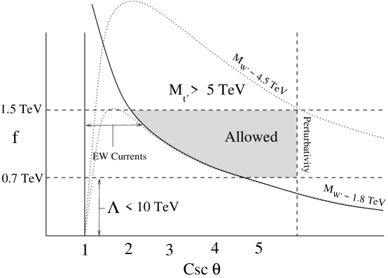
Figure 4: Sketch of the parameter space that gives adequately small non-oblique corrections. The bounds on $f$ come from naturalness considerations (upper) and the requirement that the cutoff satisfies $\Lambda\,\raise 1.29167pt\hbox{$>$\kern-7.5pt\lower 4.30554pt\hbox{$\sim$}}\,10$ TeV (lower).

In our discussion we have emphasized the usefulness of the near-oblique limit for identifying regions of parameter space that lead to acceptably small precision electroweak corrections. How close to this limit do we need to be? Focusing on the $SU(2)$ interactions, a rough answer to this question is given in Fig. 4. From this figure one can infer, for a given value of $f$, the range of values of the mixing angle $\theta$ that give small non-oblique corrections. We require $f$ to be above 700 GeV to keep the cutoff near 10 TeV (and also because for smaller values of $f$ the constraints on $\theta$ and $\theta^{\prime}$ become increasingly severe), while the upper bound on $f$ is motivated by naturalness considerations. The plot also shows a lower bound on $\theta$ from the requirement that $g_{2}$ remain perturbative. The mass of the $W^{\prime}$ ranges from roughly 1.8 to 4.5 TeV in the allowed region.

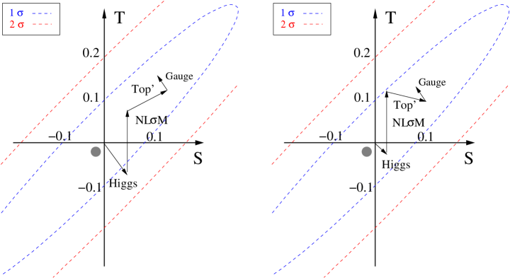
Figure 5: Contributions to the $S$ and $T$ parameters for the reference parameter values of Sec. 1.2. The dashed ellipses are roughly the $1\sigma$ and $2\sigma$ limits in the $S-T$ plane.

For points inside the allowed region of this plot, non-oblique corrections are sufficiently small that an analysis of the oblique corrections using the $S$ and $T$ parameters is meaningful. In Sec. 3.2, we calculated the contributions to $T$ from the gauge interactions (positive and small in the near-oblique limit, or absent entirely if only $U(1)_{Y}$ is gauged), the non-linear sigma model self-interactions (positive and small for $\tan\beta\simeq 1$), Higgs loops (typically negative, and growing in magnitude with the the quartic coupling $\lambda$), and top-sector loops (reasonably small for parameters that give mild radiative corrections to the Higgs mass squared, as preferred by naturalness considerations). We also calculated the contributions to $S$ and found sizable positive contributions from the top and Higgs sectors, so a positive contribution to $T$ may in fact be welcome given the shape of the $S-T$ ellipse.

In Fig. 5 we show the $S-T$ ellipse along with the various contributions to $S$ and $T$ that arise for both sets of reference values given in Sec. 1.2. The total contributions are in reasonable agreement with precision data. Certainly there are different parameter choices that lead to much larger corrections, but we believe that it is an important result that there is no intrinsic conflict between the naturalness of the Higgs potential and precision electroweak data in this theory. In the next section we give a more thorough consideration of this issue.

4 Discussion

4.1 Naturalness, Precision Electroweak, and Higgs Physics

In this section we explore the interplay between precision electroweak constraints, naturalness considerations, and Higgs physics in this model.

We focus on values of $\tan\beta$ close to one, giving small oblique corrections from the non-linear sigma model self interactions. We have already argued that these values are quite natural in this model given the approximate $SU(2)_{H,R}$ symmetries. One can express $\tan\beta$ in terms of $\delta m^{2}$, the calculable and finite radiative Higgs mass from the top sector, and $\Delta m^{2}$, the incalculable but $SU(2)_{H}$-symmetric contributions from the gauge and scalar sectors (Eq. 2.104). Choosing top-sector angles $\vartheta_{Q}$ and $\vartheta_{U}$ that minimize the top contribution, $\delta m^{2}$ can in turn be rewritten in terms of $\beta$ and $f$ (Eq. 2.94), and we can finally approximate Eq. 2.104 as

$$\cos 2\beta(1+\cos 2\beta) \simeq \frac{f^{2}}{8\Delta m^{2}},$$ (4.1)

where we have expanded around $\cos 2\beta=0$. Naturalness motivates us to concentrate on relatively small values for $\Delta m^{2}$, but if we take it too small, $\cos 2\beta$ becomes too large based on precision electroweak considerations. For our reference value $f=700$ GeV, taking $\Delta m=550$ GeV gives $\cos 2\beta\simeq 0.18$, and a reasonably small non-linear sigma model contribution to $T$ according to the discussion in Sec. 3.2.2. The same parameters give $\delta m\simeq 300$ GeV.

Before proceeding further, we note that this value for $\Delta m$ is in rough agreement with what one would expect based on the logarithmically divergent one-loop gauge and scalar contributions. For $f=700$ GeV, Fig. 4 shows that non-oblique corrections require $\theta\simeq 1/5$, in which case Eq. (2.57) gives

$$\Delta m^{2}_{\text{$SU(2)$ Gauge}}\simeq(300\text{ GeV})^{2},$$ (4.2)

while the $U(1)$ gauge contribution is negligible even with a breaking scale $\bar{f}\sim 2$ TeV. Finally, the scalar contribution of Eq. (2.70) is

$$\Delta m^{2}_{\text{Scalar}}\simeq\lambda^{2}(200\text{ GeV})^{2}.$$ (4.3)

As always, naturalness prefers larger values of $\lambda$, and depending on the contribution to $T$ from the top sector, having $\lambda\sim 2-4$ may be favorable for agreement with precision data. However even for smaller $\lambda$ the large cut-off uncertainties in these estimates make it completely reasonable to have $\Delta m\,\raise 1.29167pt\hbox{$>$\kern-7.5pt\lower 4.30554pt\hbox{$\sim$}}\,500\text{ GeV}$.

For the values of $\delta m$ and $\Delta m$ arrived at above, we find that the fine-tuning parameter introduced in Eq. 5 is

$$\kappa\simeq 0.06\,\lambda.$$ (4.4)

For a positive contribution to $T$ from the top sector, as arises for the first set of reference parameters in Sec. 1.2, large values of $\lambda$ are welcome because of the compensating corrections from the Higgs sector. In this case, the fine tuning is quite mild and lightest Higgs boson is moderately heavy. This is not to say that a light Higgs boson is disfavored. In fact, some parameters of the top sector, such as those in the second set of reference parameters of Sec. 1.2, give rise to a negative contribution to $T$ and a sizeable oblique correction from the Higgs sector is unnecessary. Small $\lambda$ and a light Higgs boson are completely consistent with precision data, although the fine tuning becomes more severe as $\lambda$ is decreased.

Positive $\Delta T$ from the Top Sector

These trends are depicted in Figs. 6 through 9 for various $\delta m$ and $\Delta m$. In these plots the contributions to $S$ and $T$ include all of those calculated in Sec. 3. For the gauge contributions we take $F=2$ TeV, $\delta\theta^{\prime}=0.1$ and $\theta=0.2$ to be sufficiently close to the near-oblique limit. Eliminating the $B^{\prime}$ by gauging only $U(1)_{Y}$ shifts the contours downwards by 0.04 in $T$.

In Figs. 6 and 7, the top contributions are calculated taking the first set of reference values $\cos^{2}\vartheta_{U}=\cos^{2}\vartheta_{Q}=2/3$.

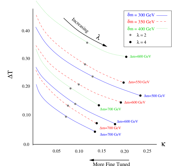
Figure 6: $T$ vs. the fine-tuning parameter $\kappa$, for several values of $\delta m$ and $\Delta m$, as the quartic coupling $\lambda$ is varied. For a given value of $\delta m$, naturalness prefers small $\Delta m$ while precision electroweak data prefer larger values. Increasing the quartic coupling significantly reduces both the fine tuning and $\Delta T$.

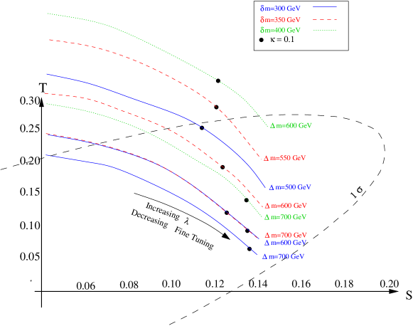
Figure 7: $S-T$ contours for the same values of $\delta m$ and $\Delta m$ as in Fig. 6. The bullets denote 10% fine tuning and the one-sigma ellipse is shown.

In Fig. 6 we see that for the Higgs mass parameters considered, $10-20$% fine tuning is required for $\lambda\sim 2-4$. The net contributions to $T$ can be reasonably small, but are certainly far from negligible. As shown in Fig. 7, increasing $\lambda$ also increases the Higgs sector’s contribution to $S$, helpful given the positive contributions to $T$ and the shape of the $S-T$ ellipse. The plot shows that there are indeed parameters that give decent agreement with precision data and only mild fine tuning.

For illustrative purposes, let us consider the Higgs spectrum for the parameters from above, $\Delta m=550$ GeV and $\delta m=300$ GeV, taking $\lambda=3$. The fine tuning is given by $\kappa=0.18$ and the oblique corrections are $(S,T)=(0.13,0.13)$. Using the fact that $\cos 2\beta$ is small, the mass of the lightest Higgs from Eq. 2.109 can be approximated as

$$m^{2}_{h^{0}}=\frac{\lambda v^{2}}{2}(1+\mathcal{O}(\cos^{2}2\beta)).$$ (4.5)

Numerically we find

$$m_{h^{0}}=297\text{ GeV}\hskip 21.68121ptm_{H^{0}}=720\text{ GeV}\hskip 21.68121ptm_{H^{\pm}}=718\text{ GeV}\hskip 21.68121ptm_{A^{0}}=779\text{ GeV}.$$ (4.6)

The charged Higgs and heavier CP even Higgs are typically nearly degenerate in the regions of parameter space that are preferred by precision electroweak data, given that $\kappa\,\raise 1.29167pt\hbox{$<$\kern-7.5pt\lower 4.30554pt\hbox{$\sim$}}\,\frac{1}{3}$.

From Eq. 2.106 one can see that the $h^{0}-H^{0}$ mixing angle $\alpha$ is typically close to $-\beta$ because $x\simeq 1-\kappa$. This means that the $h^{0}$ and $H^{0}$ couplings to fermions have no large enhancements or suppressions, because both angles are $\mathcal{O}(1)$. The couplings of the $W^{\pm}$ and $Z^{0}$ to $h^{0}$ go like $\sin(\beta-\alpha)\sim\sin 2\beta$ and are essentially unsuppressed, while the couplings to $H^{0}$ are proportional to $\cos(\beta-\alpha)\sim\cos 2\beta$, and are quite suppressed. Thus the lightest Higgs looks very much like the Standard Model Higgs in terms of its couplings.

Negative $\Delta T$ from the Top Sector

In Figs. 8 and 9 we use the second set of reference values for the top sector, $\cos^{2}\vartheta_{U}=3/4$ and $\cos^{2}\vartheta_{Q}=3/5$. The top sector gives a negative contribution to $T$ for these values, and in this case there is no tension between small $\lambda$ and precision data.

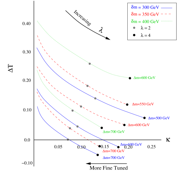
Figure 8: $T$ vs. the fine-tuning parameter $\kappa$, for several values of $\delta m$ and $\Delta m$, as the quartic coupling $\lambda$ is varied. For a given value of $\delta m$, naturalness prefers small $\Delta m$ while precision electroweak data prefer larger values. Increasing the quartic coupling significantly reduces both the fine tuning and $\Delta T$.

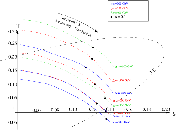
Figure 9: $S-T$ with a negative top contribution to $T$. The contours are for the same values of $\delta m$ and $\Delta m$ as in Fig. 8. The bullets denote 10% fine tuning and the one-sigma ellipse is shown.

Taking the $\Delta m^{2}$ and $\delta m^{2}$ as before, but now with $\lambda=0.5$, we find

$$m_{h^{0}}=122\text{ GeV}\hskip 21.68121ptm_{H^{0}}=718\text{ GeV}\hskip 21.68121ptm_{H^{\pm}}=718\text{ GeV}\hskip 21.68121ptm_{A^{0}}=728\text{ GeV}.$$ (4.7)

Notice that heavy Higgs spectrum is insensitive to $\lambda$. As before, the couplings of the lightest Higgs boson are Standard Model-like.

4.2 Conclusions and Outlook

In this paper we studied precision electroweak constraints on the $SU(6)/Sp(6)$ little Higgs theory. We found it useful to first identify a “near-oblique limit” in which the heavy $W^{\prime}$ and $B^{\prime}$ of the model decouple from the light two generations of fermions. Then we calculated oblique corrections that arise from the non-linear sigma model self-interactions, gauge interactions, top loops, and Higgs loops. We found parameter space with $(S,T)$ in reasonable agreement with precision data, and with only mild fine tuning in the Higgs sector, at the $10-20$% level. Non-oblique corrections involving the third generation were considered only briefly and deserve further study.

In our study we explored a number of possible modifications to the model as presented in [6]. First, we noted that an independent breaking scale for the $U(1)$ gauge interactions could be introduced without affecting other aspects of the model – in fact, it is possible to remove the $B^{\prime}$ from the theory altogether, by gauging only the Standard Model hypercharge, without introducing severe fine tuning. The additional breaking may be necessary for values of $f$ consistent with naturalness, in order to evade direct constraints from $B^{\prime}$ production. A second modification was to charge the light two generations equally under both $U(1)$ groups in order to realize the near-oblique limit. Since the third generation is charged only one $U(1)$ this leads to flavor non-universality in the couplings of the $B^{\prime}$, and the possibility of interesting flavor-changing signatures. Finally, we considered a new top sector that gives finite radiative contributions to the Higgs potential. In the appendix we also consider other alternatives for the top sector, and the oblique corrections induced by the third generation fermions change depending on the setup.

Tree-level oblique corrections arising from the non-linear sigma model structure of the theory vanish for $\tan\beta=1$. In the absence of radiative corrections from the top sector, approximate $SU(2)$ symmetries of the model guarantee that $\tan\beta$ is very close to one. In the top sector of Sec. 2.5, values for the mixing angles $\vartheta_{Q}$ and $\vartheta_{U}$ that minimize the top contribution to the Higgs mass, $\delta m^{2}$, tend to give small contributions to the $T$ parameter. These smaller values of $\delta m^{2}$ reduce the minimum gauge and scalar radiative contributions necessary for $\tan\beta$ to be consistent with precision electroweak constraints, which in turn reduces the fine tuning in the Higgs potential. For $f$ ranging from $0.7-1.5$ TeV, the values of the masses that minimize $\delta m^{2}$ are $m_{u_{H}},m_{q_{H}}\simeq 2-4$ TeV, while the other particles of the top sector have masses $m_{d_{H}},m_{q^{\prime}_{H}}\simeq 1-2$ TeV for the same parameters.

For the same range of $f$, the mass of the $W^{\prime}$ lies within $\simeq 1.8-4.5$ TeV for parameters that give adequately small non-oblique corrections. In the presence of the extra breaking scale, the mass of the $B^{\prime}$ is not tied to the others, but even for ${\overline{f}}$ as large as 2 TeV, it is quite light, with a mass of only 375 GeV. To adequately suppress non-oblique corrections associated with a $B^{\prime}$ of this mass it must couple only weakly to light fermions, which complicates collider searches.

We found that for some top sector parameters, oblique corrections from Higgs loops improve the agreement with precision data for somewhat large values of the quartic coupling $\lambda$. Larger $\lambda$ corresponds to less severe fine tuning, so in this case precision data and naturalness considerations have similar preferences. In this case the lightest Higgs boson will be somewhat heavy, though still less that $350\text{ GeV}$ given that we expect $\lambda\leq 4$. On the other hand, for other top sector parameters that give negative contributions to $T$, small $\lambda$ is equally acceptable for precision data. In this case the mass of the lightest Higgs can be near its current experimental bound. In general, the tree-level couplings of the lightest Higgs resemble those of the Standard Model Higgs. The other Higgs particles have masses of roughly 700 GeV or heavier irrespective of the quartic coupling, with the pseudoscalar being the heaviest state.

Appendix A Alternate Top Sectors

In this appendix we consider alternatives to the top sector of Sec. 2.5, which have different radiative properies and give different oblique corrections. In [6] a top sector with two separate couplings to the non-linear sigma model field was introduced,

$$\mathcal{L}_{\text{top LSS}} = y_{1}f\left(\begin{array}[]{cccc}\tilde{q}&q_{3}&\tilde{u}&0\end{array}\right)\Sigma\left(\begin{array}[]{c}0\\ 0\\ 0\\ u^{c}_{3}\end{array}\right)+y_{2}f\left(\begin{array}[]{cccc}0&q_{3}&0&0\end{array}\right)\Sigma^{*}\left(\begin{array}[]{c}\tilde{q}^{c}\\ 0\\ \tilde{u}^{c}\\ \tilde{d}^{c}\end{array}\right)$$ (A.12)

$$+y_{3}f\tilde{q}^{c}\tilde{q}+y_{4}f\tilde{u}^{c}\tilde{u}+y_{5}f\tilde{d}^{c}\tilde{d}.$$

The motivation for including both couplings was that it broke the Peccei-Quinn symmetry in the Higgs sector. But as discussed in [6], if the Peccei-Quinn symmetry is broken elsewhere, simpler setups for the third generation are possible. These are worth considering because the top sector of Eq. (A.12) has five parameters, one combination of which fixes the top mass while another fixes the $b$-term, and a detailed analysis of this setup becomes quite complicated. To simplify the analysis, note that it is possible to decouple either of the two interactions while keeping the top mass fixed and leaving the Higgs sector radiatively stable. The limits are

$$y_{2}\rightarrow 0\hskip 36.135pty_{5}\rightarrow 0\hskip 36.135pt\text{ $SU(5)_{L}$ Minimal Top Sector}$$ (A.13)

$$y_{1}\rightarrow 0\hskip 36.135pty_{4}\rightarrow 0\hskip 36.135pt\text{ $SU(4)_{R}$ Minimal Top Sector}$$ (A.14)

In the limit for the $SU(4)_{R}$ MTS, it is also necessary to decouple the additional light $SU(2)_{L}$ singlet with an interaction $\tilde{y}_{4}fu_{3}^{c}\tilde{u}$. In this appendix, we study both of these top sectors.

A.1 Summary of Other Top Sectors

Before delving into the details of these different top sectors, there are some general features that can be made. The structure of the radiative corrections to the Higgs mass is different than those of the full six-plet top sector that was studied in the paper. First, the contribution is log divergent and there are two loop quadratic divergences that make $\delta m^{2}$, the $SU(2)_{H}$ violating mass a parameter rather than a calculable coefficient. The structure of radiative corrections is of the form

$$V_{\text{1 loop top}}=-\frac{3y_{\text{top}}^{2}}{8\pi^{2}}m^{2}_{t^{\prime}}\log\frac{\Lambda^{2}}{m^{2}_{t^{\prime}}}\left(|h_{1}|^{2}+|h_{2}|^{2}\right)+\frac{3y_{\text{top}}^{2}}{8\pi^{2}}\frac{m^{2}_{\tilde{t}^{\prime}}}{\cos^{2}\vartheta}\log\frac{\Lambda^{2}}{m^{2}_{\tilde{t}^{\prime}}}|h_{2}|^{2}$$ (A.15)

where

$$m_{t^{\prime}}\simeq\frac{2y_{\text{top}}f}{\sin 2\vartheta}$$ (A.16)

is the mass of the top partner canceling the quadratic divergence from the top quark. Notice that the contribution proportional to this mass is $SU(2)_{H}$ symmetric and does not cause $\tan\beta$ to deviate from unity. The second contribution that is not $SU(2)_{H}$ symmetric could in principle be made small by taking $m^{2}_{\tilde{t}^{\prime}}$ small, making $\tan\beta$ very close to unity. This is possible because $m^{2}_{\tilde{t}^{\prime}}$ is unrelated to the top Yukawa, as the $\tilde{t}^{\prime}$ is responsible for canceling an auxiliary quadratic divergence that is not directly due to the Standard Model top quark loop, but to an interaction of the form $h_{2}^{\dagger}h_{2}t^{c}\tilde{t}$ that appears when the top Yukawa coupling is covariantize. Unfortunately, typically oblique corrections will not allow the mass of this auxiliary top partner to be much smaller than $f$.

The next general feature is that the $SU(4)_{R}$ minimal top sector typically gives a negative contribution to $T$ while the $SU(5)_{L}$ minimal top sector gives a positive contribution. Again there are log divergences to the $T$ parameter in the $SU(4)_{R}$ minimal top sector and these arise from the renormalization of the kinetic terms. However since the top sector does not preserve an $SU(6)$ chiral symmetry, these log divergences typically renormalize non-$SU(6)$ invariant kinetic terms like $\text{\,Tr\,}|\mathcal{P}D_{\mu}\Sigma|^{2}$ where $\mathcal{P}$ is a projection matrix. These effects could be important in naturalness considerations. Throughout the section the calculations have the log divergence cut-off at $\Lambda\sim 4\pi f$. The $SU(5)_{L}$ minimal top sector, because it contains only heavy singlets, does not have log divergent contributions to the T parameter.

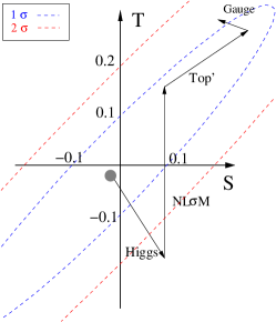
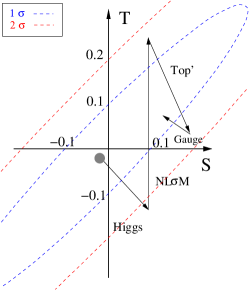
Figure 10: The dashed ellipses are roughly the $1\sigma$ and $2\sigma$ limits on the $S-T$ plane. In the $SU(5)_{L}$ minimal top sector the contribution to $T$ is positive, while in the $SU(4)_{R}$ minimal top sector the contribution to $T$ is negative. The Higgs and top contributions are important for understanding constraints on the model in these cases.

A.2 $SU(4)_{R}$ Minimal Top Sector

The $SU(4)_{R}$ MTS adds a vector like quark doublet and down-like singlet. They combine with the third generation quark doublet and up-like singlet to interact in an $SU(4)_{R}$ symmetric fashion. This global symmetry prevents one loop quadratic divergences from appearing from the top Yukawa coupling. The fermions couple to $\Sigma$ as

$$\mathcal{L}_{\text{top}}=y_{1}f\left(\begin{array}[]{cccc}\tilde{q}^{c}&0&u_{3}^{c}&\tilde{d}^{c}\end{array}\right)\Sigma^{*}\left(\begin{array}[]{c}0\\ q_{3}\\ 0\\ 0\end{array}\right)+y_{2}f\;\tilde{q}\tilde{q}^{c}+\tilde{y}_{2}f\;\tilde{d}\tilde{d}^{c}+\text{ h.c. }.$$ (A.22)

The quark doublet mixes with the vector-like fermion and can be diagonalized with mixing angles $\vartheta_{Q}$,

$$\tan\vartheta_{Q}=\frac{y_{1}}{y_{2}}\hskip 36.135pty_{\text{top}}^{-2}=|y_{1}|^{-2}+|y_{2}|^{-2},$$ (A.23)

while the masses are

$$m_{q_{H}}=\frac{2y_{\text{top}}f}{\sin 2\vartheta_{Q}}\hskip 36.135ptm_{d_{H}}=\tilde{y}_{2}f.$$ (A.24)

This top sector has the property that after electroweak symmetry breaking the $\tilde{d}^{c}$ mixes with $d_{3}\subset q_{3}$.

A.2.1 MTS Radiative Corrections

The top Yukawa preserves an $SU(4)_{R}$ chiral symmetry, preventing a quadratically divergent mass term for the Higgs from being generated at one loop. The one loop contribution from the Coleman-Weinberg potential is

$$V_{\text{eff}}=\frac{3y^{2}_{\text{top}}}{4\pi^{2}}\left(-m_{q_{H}}^{2}\log\frac{\Lambda^{2}}{m_{q_{H}}^{2}}\;(|h_{1}|^{2}+|h_{2}|^{2})+\frac{m_{d_{H}}^{2}}{\cos^{2}\vartheta_{Q}}\log\frac{\Lambda^{2}}{m_{d_{H}}^{2}}\;|h_{2}|^{2}\right).$$ (A.25)

This is the only interaction that breaks the $SU(2)_{H}$ symmetry that rotates one Higgs doublet into the other. As $m_{d}\rightarrow 0$ this contribution becomes smaller and the symmetry is restored.

A.2.2 Oblique Corrections

The minimal $SU(4)_{R}$ top sector has one heavy vector-like quark doublet and one heavy vector-like down type quark singlet. The Standard Model top doublet is a mixture of $q_{3}$ and $\tilde{q}$ with mixing angle $\vartheta_{Q}$. The mass of the heavy single $d_{H}$ is given at first order by $\tilde{y_{2}}f$. As mentioned above, the radiative corrections to the Higgs mass for this top sector have two parts (see eq A.25). One is a common contribution to $m_{1}$ and $m_{2}$, proportional to $m_{q_{H}}$, which we denote $\Delta_{\text{top}}m=\sqrt{\Delta_{\text{top}}m^{2}}$ and the other is a contribution to $m_{1}$ proportional to $m_{d_{H}}$, denoted $\delta m=\sqrt{\delta m^{2}}$. $\delta m$ is positive, so it tends to create a $\tan\beta$ that is larger than one.

We find that the contribution to $T$ is in general negative. It becomes more negative as $m_{d_{H}}$ is lowered, and do not depend very strongly on $\vartheta_{Q}$. In figure 11 we show T as a function of $\delta m$ for $f=700\text{ GeV}$, and $\vartheta_{Q}=\pi/4$ assuming that the log in eq. A.25 is 5. This is only an illustration of the typical size of $\delta m$ as log divergent contributions are not calculable. The choice of $\vartheta_{Q}$ minimize $\Delta m$ as well as $\delta m$. We show also in figure 11 $T$ vs $S$ for the $f=700$, $\tan\beta=1$ and $\vartheta_{Q}=\pi/4$ when $\delta m$ is scanned over. We see that the contributions to S can be quite important.

Figure 11: T as a function of $\delta m$ for $f=700\text{ GeV}$, $\vartheta_{Q}=\pi/4$ for $\tan\beta$ of $0.8,1$ and $1.2$. This correspond to $\Delta_{\text{top}}m$ of $506,617$ and $753$ GeV respectively. On the right hand side we show T vs S for $f=700\text{ GeV}$, $\tan\beta=1$ and $\vartheta_{Q}=\pi/4$

A.3 $SU(5)_{L}$ Minimal Top Sector

The $SU(5)_{L}$ MTS adds an up-like singlet and a doublet to the top sector. These couple to $\Sigma$ with the top quark, $q_{3}$ and $u_{3}^{c}$, through

$$\mathcal{L}_{\text{top}}=y_{1}f\left(\begin{array}[]{cccc}0&0&0&u_{3}^{c}\end{array}\right)\Sigma\left(\begin{array}[]{c}q\\ \tilde{q}\\ \tilde{u}\\ 0\end{array}\right)+\tilde{y}_{2}f\;\tilde{q}\tilde{q}^{c}+y_{2}f\;\tilde{u}\tilde{u}^{c}+\text{ h.c. }$$ (A.31)

The quark doublet mixes with the vector-like fermion and can be diagonalized with mixing angles $\vartheta_{Q}$,

$$\tan\vartheta_{U}=\frac{y_{1}}{y_{2}}\hskip 36.135pty_{\text{top}}^{-2}=|y_{1}|^{-2}+|y_{2}|^{-2},$$ (A.32)

while the masses are

$$m_{q_{H}}=\frac{2y_{\text{top}}f}{\sin 2\vartheta_{Q}}\hskip 36.135ptm_{u_{H}}=\tilde{y}_{2}f.$$ (A.33)

A.3.1 Radiative Corrections

The top Yukawa preserves an $SU(5)_{L}$ chiral symmetry, preventing a quadratically divergent mass term for the Higgs doublets from being generated at one loop. The one loop contribution from the Coleman-Weinberg potential is

$$V_{\text{eff}}=\frac{3y^{2}_{\text{top}}}{4\pi^{2}}\left(-m_{q_{H}}^{2}\log\frac{\Lambda^{2}}{m_{q_{H}}^{2}}\;(|h_{1}|^{2}+|h_{2}|^{2})+\frac{m_{u_{H}}^{2}}{\cos^{2}\vartheta_{U}}\log\frac{\Lambda^{2}}{m_{d_{H}}^{2}}\;|h_{2}|^{2}\right).$$ (A.34)

Only the second term breaks the $SU(2)_{H}$ symmetry that rotates one Higgs doublet into the other. As $m_{u}\rightarrow 0$ this contribution becomes smaller and the symmetry is restored.

A.3.2 Oblique Corrections

The $SU(5)_{L}$ minimal top sector has one heavy doublet, and one heavy up-type singlet. At $0^{\text{th}}$ order, the doublet doesn’t mix, and the right-handed top is a mixture of $u_{3}$ and $\tilde{u}$ with mixing angle $\vartheta_{U}$. Similarly to the $SU(4)_{R}$ minimal top sector, the radiative corrections from the top sector gives a contribution common to $h_{1}$ and $h_{2}$, $\Delta m$ proportional to $m_{u_{H}}$, and a contribution to $h_{1}$, $\delta m$ proportional to $m_{q_{H}}$.

We find that the contribution to T in the $SU(5)_{L}$ minimal top sector are quite important. They tend to decrease as $\vartheta_{U}$ is made small or as $y_{2}$ become large. Both of these limits however, tend to increase the radiative corrections to the Higgs mass. We show in figure 12, T as a function of $m_{q_{H}}$ for $f=700\text{ GeV}$ and various values of $\tan\beta$. The dependence on $\vartheta_{U}$ is very mild.

Figure 12: $T$ as a function of $m_{q_{H}}$ for $f=700\text{ GeV}$, $m_{u_{H}}=2\text{ TeV }$ and $\tan\beta$ of $0.8$, $1$ and $1.2$. On the right hand side we show $T$ as a function of $S$ for $f=700\text{ GeV}$, $\tan\beta=1$, $m_{u_{H}}=2\text{ TeV }$ and $m_{q_{H}}$ going from $500\text{ GeV}$ to $3.5\text{ TeV }$.

We have also calculated the correction to the $S$ parameter and found it to be quite small. Figure 12 also shows $T$ as a function of $S$ for $f=700\text{ GeV}$, $\tan\beta=1$, $m_{u_{H}}=2\text{ TeV }$ and a range of values of $m_{q_{H}}$.

References

- [1] N. Arkani-Hamed, A. G. Cohen and H. Georgi, Phys. Lett. B 513, 232 (2001)
- [2] N. Arkani-Hamed, A. G. Cohen, T. Gregoire and J. G. Wacker, arXiv:hep-ph/0202089.
- [3] N. Arkani-Hamed, A. G. Cohen, E. Katz, A. E. Nelson, T. Gregoire and J. G. Wacker, arXiv:hep-ph/0206020.
- [4] T. Gregoire and J. G. Wacker, arXiv:hep-ph/0206023.
- [5] N. Arkani-Hamed, A. G. Cohen, E. Katz and A. E. Nelson, JHEP 0207, 034 (2002)
- [6] I. Low, W. Skiba and D. Smith, Phys. Rev. D 66, 072001 (2002) [arXiv:hep-ph/0207243].
- [7] D. E. Kaplan and M. Schmaltz, arXiv:hep-ph/0302049.
- [8] J. G. Wacker, arXiv:hep-ph/0208235.
- [9] M. Schmaltz, arXiv:hep-ph/0210415.
- [10] A. E. Nelson, arXiv:hep-ph/0304036.
- [11] R. S. Chivukula, N. Evans and E. H. Simmons, arXiv:hep-ph/0204193.
- [12] J. L. Hewett, F. J. Petriello and T. G. Rizzo, arXiv:hep-ph/0211218.
- [13] C. Csaki, J. Hubisz, G. D. Kribs, P. Meade and J. Terning, arXiv:hep-ph/0211124.
- [14] S. Chang and J. G. Wacker, arXiv:hep-ph/0303001.
- [15] C. Csaki, J. Hubisz, G. D. Kribs, P. Meade and J. Terning, arXiv:hep-ph/0303236.
- [16] G. D. Kribs, arXiv:hep-ph/0305157.
- [17] G. Burdman, M. Perelstein and A. Pierce, arXiv:hep-ph/0212228.
- [18] T. Han, H. E. Logan, B. McElrath and L. T. Wang, arXiv:hep-ph/0301040.
- [19] B. Grinstein and M. B. Wise, Phys. Lett. B 265, 326 (1991).
- [20] C. P. Burgess, S. Godfrey, H. Konig, D. London and I. Maksymyk, Phys. Rev. D 49, 6115 (1994) [arXiv:hep-ph/9312291].
- [21] P. Bamert, C. P. Burgess, J. M. Cline, D. London and E. Nardi, Phys. Rev. D 54, 4275 (1996) [arXiv:hep-ph/9602438].
- [22] M. S. Chanowitz, Phys. Rev. Lett. 87, 231802 (2001) [arXiv:hep-ph/0104024].
- [23] M. S. Chanowitz, Phys. Rev. D 66, 073002 (2002) [arXiv:hep-ph/0207123].
- [24] R. Barbieri and A. Strumia, Phys. Lett. B 462, 144 (1999) [arXiv:hep-ph/9905281].
- [25] M. E. Peskin and J. D. Wells, Phys. Rev. D 64, 093003 (2001) [arXiv:hep-ph/0101342].