Unintegrated parton distributions of pions and nucleons from the CCFM equations in the single-loop approximation

Agnieszka Gawron, Jan Kwieciński, and Wojciech Broniowski

The H. Niewodniczański Institute of Nuclear Physics, PL-31342 Cracow, Poland

The unintegrated quark and gluon distributions in the pion and nucleon are analysed using the CCFM equations in the single-loop approximation. We utilise the transverse-coordinate (or impact-parameter) representation which diagonalises the equations and study in detail the dependence on the transverse coordinate induced by the CCFM evolution. We find considerable broadening of the transverse-momentum distributions with an increasing magnitude of the hard scale, $Q$. For instance, at the Bjorken $x=0.1$ the root mean squared transverse momentum of the gluons is enhanced by about 1 GeV when evolved from the the initial low scale to $Q^{2}=10~{}{\rm GeV}^{2}$, and by about 2 GeV when evolved up to to $Q^{2}=100~{}{\rm GeV}^{2}$. The broadening effect is enhanced with decreasing Bjorken $x$, and is stronger for the gluons than for the quarks. Analytic solution for the average transverse momentum corresponding to the $x$-moments of the distributions is obtained. The parton luminosities are also discussed.

1 Introduction

Parton distributions are fundamental and universal quantities of the QCD-improved parton model. They depend on the longitudinal momentum fraction of the parent hadron, $x$, as well as on the hard scale of the process, $Q$. The inclusive cross-sections describing hard processes are governed by the (collinear) factorisation theorem expressing those cross-sections as convolutions of partonic distributions and hard (partonic) cross-sections [1]. On the other hand, less inclusive measurements are often sensitive to the transverse momenta of the partons and require an introduction of the unintegrated parton distributions, i.e. distributions which are not integrated over the transverse momentum of the parton [2, 3, 4, 5, 6, 7, 8, 9, 10, 11]. These unintegrated distributions depend then upon the transverse momentum of the parton besides the dependence on $x$ and $Q$. Typical cases where the information on the transverse momentum of partons is needed are the prompt photon production, or the transverse momentum distributions of the Drell-Yan lepton pairs, $W^{\pm}$ and $Z^{0}$ bosons, etc. The unintegrated parton distributions are also needed in the calculations made within the $k_{T}$-factorisation framework [12, 13, 14, 15, 16].

The unintegrated parton distributions are described by the Catani-Ciafaloni-Fiorani- Marchesini (CCFM) equations [17, 18, 19, 20, 21, 22, 23, 24, 25, 26, 27] which are based on the quantum coherence implying angular ordering along the partonic cascade [28]. In the so-called single-loop approximation [19, 20], adequate for large and moderately small values of $x$ (say, $x>0.01$), the CCFM equations reproduce the conventional leading-order DGLAP equations for the integrated distributions. Thus, they may be viewed as an extension of the DGLAP evolution which allows to investigate more general quantities.

The purpose of this paper is to analyse in detail the unintegrated parton distributions of pions and nucleons. To this aim we explore the system of the CCFM equations in the single loop approximation utilising the transverse-coordinate representation of the parton distributions. The transverse-coordinate, denoted in this paper by $b$, is a variable conjugate to the transverse momentum of the parton. It has been widely used in the study of the soft gluon resummation effects in the $e^{+}e^{-}$ collisions [29, 30], in the transverse-momentum distributions of the Drell-Yan pairs or gauge bosons [31], etc. The formalism adopted in our analysis is similar to methods used in those studies. An important merit of our use of the transverse-coordinate representation is the fact that it diagonalises the system of the CCFM equations in the single-loop approximation [32, 33]. In practice, this means that the equations are solved independently for each value of $b$. Also, in this approximation the non-perturbative effects encoded in the choice of the initial dependence on $b$ at the reference scale $Q_{0}$ (the profile function) factorise in the solution at a scale $Q$. This input profile introduces the damping factor for large values of $b$ that makes it possible to extend smoothly the partonic $k_{T}$-distributions down to the point $k_{T}=0$. The CCFM evolution changes the dependence on $b$ and leads to significant broadening of the transverse momentum distributions. The average transverse momentum squared grows approximately linearly with $Q^{2}$ (modulo logarithmic corrections). The effect is strongest for gluons, when e.g. for $Q^{2}=100~{}{\rm GeV}^{2}$ the CCFM evolution is found to generate $\langle k_{T}^{2}\rangle_{\rm evol}^{1/2}$ about $2.3~{}{\rm GeV}$ for $x=0.1$ and $3.2~{}{\rm GeV}$ for $x=0.01$. These numbers should be compared to the initial spreading, $\langle k_{T}^{2}\rangle_{F}$, which is typically assumed to be in the range of $(0.5-1~{}{\rm GeV})$. Broadening of the $k_{T}$ distribution corresponds to the development of the long-range tail in the distribution at large $k_{T}$.

The average transverse momenta squared can be expressed in terms of the logarithmic derivative of the distributions in the $b$ representation at $b=0$. Factorisation of the input profile implies that the average transverse momentum squared of the parton is the sum of the ’primordial’ (non-perturbative) component at $Q_{0}$ and the term generated by the evolution. The unintegrated parton distributions are constrained by the integrated distributions which correspond to the integrals of the unintegrated distributions over the transverse momentum squared of the partons. In order to make our analysis realistic we use constraints implied by the results of the global LO QCD analysis [34, 35] for the integrated distributions of pions and nucleons. To be precise, we take the same parametrisation of the starting integrated distributions as those used in [34, 35] and assume, as an educated guess, a Gaussian transverse momentum distribution, uniform for gluons and quarks . Combining this assumption with the evolution from the CCFM equations in the single-loop approximation one should get a set of realistic unintegrated parton distributions hadrons. These can be used in phenomenological applications in the mentioned region of large and moderately small values of $x$, where the single-loop approximation is expected to be adequate.

The content of our paper is as follows: In the next section we recall the system of the CCFM equations in the single-loop approximation and discuss its transverse coordinate representation. In Sec. 3 we discuss the unintegrated parton distributions of pions and nucleons which follow from the numerical solution of the CCFM equations in the single-loop approximation. We present our results for the $b$ profiles and for the transverse-momentum distributions, as well as discuss the increase of the average transverse momentum with the increasing magnitude of the hard scale, $Q$, at different values of $x$. In Sec. 4 we discuss the moments of the $b$ profiles and present results for the average transverse momenta squared, $<k_{T}^{2}(n,Q^{2})>_{i}$, for the $n$th moment for partons of species $i$. We also derive (semi)analytic expressions for $<k_{T}^{2}(n,Q^{2})>_{i}$. In Sec. 5 we discuss partonic luminosities and, finally, in Sec. 6 we give a summary of our results.

2 CCFM equations in the single loop approximation

The original Catani-Ciafaloni-Fiorani-Marchesini (CCFM) equation [17, 18] for the unintegrated, scale-dependent gluon distribution $f_{G}(x,k_{T},Q)$, which is generated by the sum of ladder diagrams with angular ordering along the chain, has the following form:

$$f_{G}(x,k_{T},Q) = \tilde{f}_{G}^{0}(x,k_{T},Q)+\int{d^{2}\mbox{\boldmath${q}$}\over\pi q^{2}}\int_{x}^{1}{dz\over z}\Theta(Q-qz)\Theta(q-q_{0}){\alpha_{s}\over 2\pi}\Delta_{S}(Q,q,z)$$ (1)

$$\times \left[2N_{c}\Delta_{NS}(k_{T},q,z)+{2N_{c}z\over(1-z)}f\left({x\over z},|\mbox{\boldmath${k}$}_{t}+(1-z)\mbox{\boldmath${q}$}|,q\right)\right],$$

where $\Delta_{S}(Q,q,z)$ and $\Delta_{NS}(k_{T},q,z)$ are the Sudakov and non-Sudakov form factors,

$$\Delta_{S}(Q,q,z) = \exp\left[-\int_{(qz)^{2}}^{Q^{2}}{dp^{2}\over p^{2}}{\alpha_{s}\over 2\pi}\int_{0}^{1-q_{0}/p}dzzP_{gg}(z)\right],$$ (2)

$$\Delta_{NS}(k_{T},q,z) = \exp\left[-\int_{z}^{1}{dz^{\prime}\over z^{\prime}}\int_{(qz^{\prime})^{2}}^{k_{T}^{2}}{dp^{2}\over p^{2}}{2N_{c}\alpha_{s}\over 2\pi}\right].$$ (3)

The variables $x$, $k_{T}$, and $Q$ denote the longitudinal momentum fraction, the transverse momentum of the gluon, and the hard scale, respectively. The latter is defined in terms of the maximum emission angle [10, 17]. The constraint $\Theta(Q-qz)$ in Eq. (1) reflects the angular ordering, and the inhomogeneous term, $\tilde{f}^{0}(x,k_{T},Q)$, is related to the input non-perturbative gluon distribution. It also contains effects of both the Sudakov and non-Sudakov form-factors [22].

Equation (1) in a sense interpolates between a fragment of the DGLAP evolution at large $x$ and the BFKL dynamics at small $x$. To be precise, it contains only the $g\rightarrow gg$ splittings and only those parts of the splitting function $P_{gg}(z)$ which are singular at either $z\rightarrow 1$ or $z\rightarrow 0$. In order to make the CCFM framework more realistic in the region of large and moderately small values of $x$ we make use of the following extension [33]:

1. We introduce, besides the unintegrated gluon distributions $f_{G}(x,k_{T},Q)$, also the unintegrated quark and antiquark gluon distributions, $f_{q_{i}}(x,k_{T},Q)$ and $f_{\bar{q}_{i}}(x,k_{T},Q)$.

2. We include, in addition to the $g\rightarrow gg$ splittings, also the the $q\rightarrow gq$, $\bar{q}\rightarrow g\bar{q}$, and $g\rightarrow\bar{q}q$ transitions along the chain.

3. We take into account the complete splitting functions $P_{ab}(z)$, and not only their singular parts.

In the region of large and moderately small values of the parameter $x$ ($x\geq 0.01$ or so) one can introduce the single-loop approximation that corresponds to the following replacements:

$$\Theta(Q-qz) \rightarrow \Theta(Q-q),$$

$$\Delta_{NS}(k_{T},q,z) \rightarrow 1.$$ (4)

It is also useful to ’unfold’ the Sudakov form factor such that the real emission and virtual terms appear on an equal footing in the corresponding evolution equations. Finally, the unfolded system of the CCFM equations in the single-loop approximation has the following form:

$$f_{NS}^{i}(x,k_{T},Q) = f^{i0}_{NS}(x,k_{T})+\int_{0}^{1}dz\int{d^{2}q\over\pi q^{2}}{\alpha_{s}(q^{2})\over 2\pi}\Theta(q^{2}-q_{0}^{2})\Theta(Q-q)P_{qq}(z)$$

$$\times \left[\Theta(z-x)f_{NS}^{i}\left({x\over z},k^{\prime}_{T},q\right)-f_{NS}^{i}(x,k_{T},q)\right],$$

$$f_{S}(x,k_{T},Q) = f_{S}^{0}(x,k_{T})+\int_{0}^{1}dz\int{d^{2}q\over\pi q^{2}}{\alpha_{s}(q^{2})\over 2\pi}\Theta(q^{2}-q_{0}^{2})\Theta(Q-q)$$

$$\times \bigg{\{}\Theta(z-x)\left[P_{qq}(z)f_{S}\left({x\over z},k^{\prime}_{T},q\right)+P_{qg}(z)f_{G}\left({x\over z},k^{\prime}_{T},q\right)\right]-P_{qq}(z)f_{S}(x,k_{T},q)\bigg{\}},$$

$$f_{G}(x,k_{T},Q) = f_{G}^{0}(x,k_{T})+\int_{0}^{1}dz\int{d^{2}q\over\pi q^{2}}{\alpha_{s}(q^{2})\over 2\pi}\Theta(q^{2}-q_{0}^{2})\Theta(Q-q)$$

$$\times \bigg{\{}\Theta(z-x)\left[P_{gq}(z)f_{S}\left({x\over z},Q^{\prime}_{t},q\right)+P_{gg}(z)f_{G}\left({x\over z},Q^{\prime}_{t},q\right)\right]\bigg{.}$$

$$-\bigg{.}\big{[}zP_{gg}(z)+zP_{qg}(z)\big{]}f_{G}(x,k_{T},q)\bigg{\}},$$

where

$${\bf k^{\prime}_{T}}={\bf k_{T}}+(1-z){\bf q}.$$ (8)

The functions $f_{NS}^{i}(x,k_{T},Q)$ are the unintegrated non-singlet quark distributions, while the unintegrated singlet distribution, $f_{S}(x,k_{T},Q)$, is defined as

$$f_{S}(x,k_{T},Q)=\Sigma_{i=1}^{f}[f_{q_{i}}(x,k_{T},Q)+f_{\bar{q}_{i}}(x,k_{T},Q)]$$ (9)

The functions $P_{ab}(z)$ are the LO splitting functions corresponding to real emissions, i.e.:

$$P_{qq}(z) = {4\over 3}{1+z^{2}\over 1-z},$$ (10)

$$P_{qg}(z) = N_{f}[z^{2}+(1-z)^{2}],$$ (11)

$$P_{gq}(z) = {4\over 3}{1+(1-z)^{2}\over z},$$ (12)

$$P_{gg}(z) = 2N_{c}\left[{z\over 1-z}+{1-z\over z}+z(1-z)\right].$$ (13)

where $N_{f}$ and $N_{c}$ denote the number of flavours and colours, respectively. After integrating over $d^{2}{\bf k_{T}}$ on both sides of Eqs. (2 - 2) we get the usual DGLAP equations for the integrated parton distributions $p_{k}(x,Q^{2})$, defined by

$$xp_{k}(x,Q^{2})=\int_{0}^{\infty}dk_{T}^{2}f_{k}(x,k_{T},Q).$$ (14)

Equations (2)-(2) can be diagonalised by the Fourier-Bessel transform,

$$f_{k}(x,k_{T},Q) = \int_{0}^{\infty}dbbJ_{0}(k_{T}b)\bar{f}_{k}(x,b,Q),$$ (15)

$$\bar{f}_{k}(x,b,Q) = \int_{0}^{\infty}dk_{T}k_{T}J_{0}(k_{T}b)f_{k}(x,k_{T},Q),$$ (16)

where $k=NS$, $S$, or $g$, and $J_{0}(u)$ is the Bessel function. At $b=0$ the functions $\bar{f}_{k}(x,b,Q)$ are related to the integrated distributions $p_{i}(x,Q^{2})$,

$$\bar{f}_{k}(x,b=0,Q)={1\over 2}xp_{k}(x,Q^{2}).$$ (17)

The corresponding evolution equations for $\bar{f}_{NS}(x,b,Q)$, $\bar{f}_{S}(x,b,Q)$, and $\bar{f}_{g}(x,b,Q)$, equivalent to Eqs. (2) - (2) read

$$Q^{2}{\partial\bar{f}_{NS}(x,b,Q)\over\partial Q^{2}}=$$

$${\alpha_{s}(Q^{2})\over 2\pi}\int_{0}^{1}dzP_{qq}(z)\left[\Theta(z-x)J_{0}[(1-z)Qb]\bar{f}_{NS}\left({x\over z},b,Q\right)-zP_{qq}(z)\bar{f}_{NS}(x,b,Q)\right],$$ (18)

$$Q^{2}{\partial\bar{f}_{S}(x,b,Q)\over\partial Q^{2}}=$$

$${\alpha_{s}(Q^{2})\over 2\pi}\int_{0}^{1}dz\bigg{\{}\Theta(z-x)J_{0}[(1-z)Qb]\left[P_{qq}(z)\bar{f}_{S}\left({x\over z},b,Q\right)+P_{qg}(z)\bar{f}_{G}\left({x\over z},b,Q\right)\right]\bigg{.}$$

$$\bigg{.}-[zP_{qq}(z)+zP_{gq}(z)]\bar{f}_{S}(x,b,Q)\bigg{\}},$$ (19)

$$Q^{2}{\partial\bar{f}_{G}(x,b,Q)\over\partial Q^{2}}=$$

$${\alpha_{s}(Q^{2})\over 2\pi}\int_{0}^{1}dz\bigg{\{}\Theta(z-x)J_{0}[(1-z)Qb]\left[P_{gq}(z)\bar{f}_{S}\left({x\over z},b,Q\right)+P_{gg}(z)\bar{f}_{G}\left({x\over z},b,Q\right)\right]\bigg{.}$$

$$\bigg{.}-[zP_{gg}(z)+zP_{qg}(z)]\bar{f}_{G}(x,b,Q)\bigg{\}},$$ (20)

with the initial conditions

$$\bar{f}_{k}(x,b,Q_{0})=\bar{f}_{k}^{0}(x,b).$$ (21)

In our analysis of the CCFM equations we assume, for simplicity and from the lack of detailed experimental knowledge, a factorisable form of the initial conditions (21)

$$\bar{f}_{k}^{0}(x,b)={1\over 2}F(b)xp_{k}(x,Q_{0}^{2}).$$ (22)

Other, more complicated and non-factorisable initial conditions may be explored with no difficulty as well. The input profile function, $F(b)$, is linked through the Fourier-Bessel transform (16) to the non-perturbative $k_{T}$ distribution at the scale $Q_{0}$. At $b=0$ we have the normalisation condition for the profile function, $F(0)=1$.

3 Unintegrated parton distributions in the pion and nucleon

Since the initial condition for the QCD evolution, Eq. (22), assumes a uniform dependence on the profile function $F(b)$ for all distribution functions $f_{i}$, it is convenient to factorise this function by introducing the ’tilde’ distributions,

$$\tilde{f}_{i}(x,b,Q)=\bar{f}_{i}(x,b,Q)/F(b),\;\;\;\;\;\;i={\rm G,S,NS}.$$ (23)

The evolution equations (18-20) can then be written in terms of the $\tilde{f}$ functions only. In other words, all dynamical information on the $b$-dependence, generated by the evolution and linked to the $Q$ and $x$ variables, is contained in the $\tilde{f}$ functions, while the uniform initial profile $F(b)$ is carried over as a multiplicative factor and is decoupled from the dynamics. Certainly, we may choose different profiles $F(b)$, which affects directly the shape of the unintegrated distribution functions, nevertheless the evolution is independent of this choice, as long as the factorisation is assumed. For this reason we first present the numerical results for the scaled functions $\tilde{f}_{i}(x,b,Q)$.

The evolution equations for the $\tilde{f}$ functions are solved numerically. The method used is based on the discretisation made with the help of the Chebyshev polynomials and is an extension of the method developed in [36] for the solution of the DGLAP equations.

Figure 1 shows the solutions of Eqs. (18-20) for the case of the pion with the LO Glück-Reya-Schienbein (GRS) distributions [34] taken at the initial scale $Q_{0}^{2}=0.26~{}{\rm GeV}^{2}$. The left and right sides of the figure display the results for $x=0.1$ and $x=0.01$, i.e. moderately large and moderately small values of the Bjorken variable. We show, from top to bottom, the distributions $\tilde{f}_{G}$, $\tilde{f}_{S}$, and $\tilde{f}_{NS}$, plotted as functions of the transverse coordinate, $b$. The various types of lines indicate consecutive values of the momentum $Q$, with the solid line corresponding to the initial scale of the GRS parameterisation, $Q^{2}=Q_{0}^{2}=0.26~{}{\rm GeV}^{2}$ [34], and the dashed, dash-dotted and dotted lines denoting results for $Q^{2}=1~{}{\rm GeV}^{2}$, $10~{}{\rm GeV}^{2}$, and $100~{}{\rm GeV}^{2}$, respectively. The original distributions at $Q=Q_{0}$ are flat in $b$, since we use the rescaled functions (23). We note immediately from the figure that the increase of $Q$ results in sharp peaking of the distributions at $b=0$, with the effect stronger at the smaller value of $x$. The shrinkage of the distributions in $b$ is most prominent for the gluons. For instance, for the gluons at $x=0.01$ the curves drop to half of the values at $b=0$ around $b=2$, $1.2$, and $0.6~{}{\rm GeV}^{-1}$ for $Q^{2}=1$, $10$, and $100~{}{\rm GeV}^{2}$, respectively. To the extent these distributions can be approximated with a Gaussian, that would correspond to widths in the transverse momentum of about $0.8~{}{\rm GeV}$, $1.4~{}{\rm GeV}$, and $3~{}{\rm GeV}$, respectively. The transverse-momentum distributions will be discussed in detail in the following parts of the paper. At the values of $x$ displayed in Fig. 1 the shrinking effect in $b$ is similar for the singlet and non-singlet quark distributions.

Figure 1: Solutions of the CCFM equations in the single-loop approximation, Eqs. (18-20), for the unintegrated partonic distribution functions in the pion. The gluon, $\tilde{f}_{G}$, quark singlet, $\tilde{f}_{S}$, and quark non-singlet distributions, $\tilde{f}_{NS}$, are plotted as functions of the transverse coordinate, $b$. The left and right parts are for $x=0.1$ and $x=0.01$, respectively. The solid lines correspond to the initial scale of the GRS parameterisation, $Q^{2}=Q_{0}^{2}=0.26~{}{\rm GeV}^{2}$ [34], while the dashed, dash-dotted and dotted lines correspond to $Q^{2}=1~{}{\rm GeV}^{2}$, $10~{}{\rm GeV}^{2}$, and $100~{}{\rm GeV}^{2}$, respectively.

We note that for the case of gluons at $x=0.01$ the function $\tilde{f}_{G}$ becomes negative above $b\sim 4~{}{\rm GeV}^{-1}$. To our knowledge, this poses no physical problems. Positivity is required for the unintegrated distributions in the transverse-momentum space, since then the positivity of cross-sections, which are physical quantities, is guaranteed. The Fourier-Bessel transform of a positive function, however, need not be positive itself. We will see shortly that in the transverse-momentum space the distributions are positive. The effect of negative $\tilde{f}_{G}$ at larger $b$ and small $x$ is an artifact of the valence-like input for the gluons in the parameterisations of Refs. [34, 35], and can be understood as follows: At small $x$ the evolution equation (20) is dominated on the right-hand side by the gluon contribution, hence can be approximated with the following form:

$$Q^{2}{\partial\tilde{f}_{G}(x,b,Q)\over\partial Q^{2}}=$$

$${\alpha_{s}(Q^{2})\over 2\pi}\int_{0}^{1}dzJ_{0}[(1-z)Qb]\left\{P_{gg}(z)\tilde{f}_{G}\left({x\over z},b,Q\right)-[zP_{gg}(z)+zP_{qg}(z)]\tilde{f}_{G}(x,b,Q)\right\}$$

$$-\{zP_{qg}(z)+zP_{gg}(z)[1-J_{0}((1-z)Qb)]\tilde{f}_{G}(x,b,Q)\}$$ (24)

At small $x$ the dominant region of integration in the first term on the right-hand side of Eq. (24) is $x<z<<1$, hence we may approximate $1-z$ by $1$ in the argument of the Bessel function in this term. The solution of Eq. (24) with the initial condition

$$\tilde{f}_{G}(x,b,Q_{0})={1\over 2}xg(x,Q_{0}^{2})$$ (25)

then reads

$$\tilde{f}_{G}(x,b,Q_{0})={1\over 2}T_{g}(b,Q)xg(x,Q_{\rm eff}^{2}(b,Q)),$$ (26)

where

$$T_{g}(b,Q)=\exp\left\{\int_{Q_{0}^{2}}^{Q^{2}}{dq^{2}\over q^{2}}{\alpha_{s}(q^{2})\over 2\pi}\int_{0}^{1}dz\left[zP_{qg}(z)+zP_{gg}(z)[1-J_{0}((1-z)qb)]\right]\right\}$$ (27)

and $Q_{\rm eff}^{2}(b,Q)$ is obtained from the following implicit equation:

$$\int_{Q_{0}^{2}}^{Q_{\rm eff}^{2}(b,Q)}{dq^{2}\over q^{2}}{\alpha_{s}(q^{2})\over 2\pi}=\int_{Q_{0}^{2}}^{Q^{2}}{dq^{2}\over q^{2}}{\alpha_{s}(q^{2})\over 2\pi}J_{0}(qb).$$ (28)

The function $xg(x,Q^{2})$ is the integrated gluon distribution corresponding to the solution of equation (24) at $b=0$ with the initial condition $xg(x,Q_{0}^{2})$. At sufficiently large $b$ the integral on the right-hand side of Eq. (28) becomes negative, which gives $Q_{\rm eff}^{2}(b,Q)<Q_{0}^{2}$, and the effective ’backward’ evolution of the valence gluons gives a negative $xg(x,Q_{\rm eff}^{2})$ for sufficiently small $x$ and for $Q_{\rm eff}^{2}(b,Q)$ sufficiently smaller than $Q_{0}^{2}$. This is the technical reason for the behaviour seen in Fig. 1.

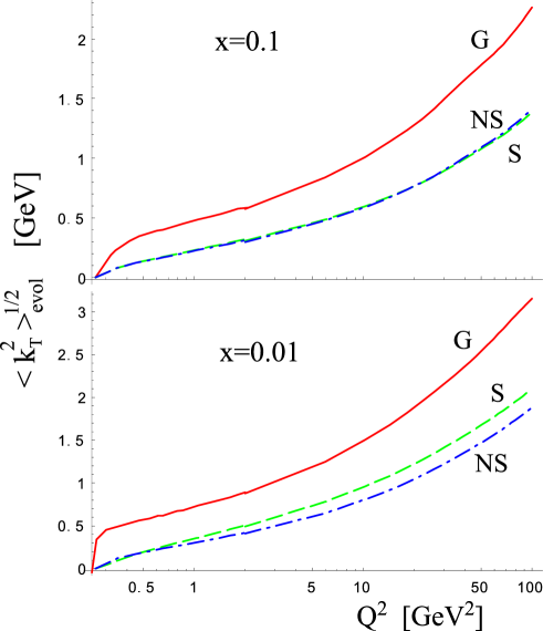
Figure 2: The dynamically-generated root mean-squared transverse momentum of unintegrated partonic distribution functions in the pion, plotted as a function of $Q^{2}$. The top and bottom parts correspond to x=0.1 and x=0.01, respectively. The solid, dashed, and dot-dashed lines denote gluons, singlet quarks, and non-singlet quarks. The CCFM equations in the single-loop approximation with the initial GRS condition [34] at the scale $Q^{2}=Q_{0}^{2}=0.26~{}{\rm GeV}^{2}$ are used for the evolution.

The mean squared transverse momentum for a given distribution is equal to

$$\langle k_{T}^{2}(x,Q^{2})\rangle_{i}\equiv\frac{\int d^{2}k_{T}\,k_{T}^{2}f_{i}(x,k_{T},Q)}{\int d^{2}k_{T}\,f_{i}(x,k_{T},Q)}=-4\left.\frac{d/db^{2}\,f_{i}(b,x,Q)}{f_{i}(b,x,Q)}\right|_{b=0},$$ (29)

where the last equality follows from the expansion $J_{0}(z)=1-\frac{1}{4}z^{2}+\dots$. Through the use of the decomposition (23) we may immediately write

$$\langle k_{T}^{2}(x,Q^{2})\rangle_{i} = \langle k_{T}^{2}\rangle_{F}+\langle k_{T}^{2}(x,Q^{2})\rangle_{\rm i,evol},$$ (30)

$$\langle k_{T}^{2}\rangle_{F} = -4\left.\frac{d/db^{2}\,F(b)}{F(b)}\right|_{b=0},$$

$$\langle k_{T}^{2}(x,Q^{2})\rangle_{\rm i,evol} = -4\left.\frac{d/db^{2}\,\tilde{f}_{i}(b,x,Q)}{\tilde{f}(b,x,Q)}\right|_{b=0},$$ (31)

which means that the total mean squared transverse momentum is the sum of the contribution from the profile $F$, which is constant and corresponds to the width at the initial scale $Q=Q_{0}$, and the piece $\langle k_{T}^{2}\rangle_{\rm i,evol}$, which is due entirely to the evolution and is independent of the profile $F$. Because of these features we concentrate on $\langle k_{T}^{2}\rangle_{\rm evol}$ in the discussion below.

In Fig. 2 we show $\langle k_{T}^{2}\rangle^{1/2}_{\rm evol}$, plotted as a function of $Q^{2}$, for $x$=0.1 (top) and $x$=0.01 (bottom). The solid, dashed, and dot-dashed lines denote gluons, singlet, and non-singlet quarks, respectively. Again, we clearly note the spreading effect with increasing $Q^{2}$. The effect is strongest for gluons, which at $Q^{2}=100~{}{\rm GeV}^{2}$ achieve $\langle k_{T}^{2}\rangle_{\rm evol}^{1/2}$ about $2.3~{}{\rm GeV}$ for $x=0.1$ and $3.2~{}{\rm GeV}$ for $x=0.01$. However, even at moderate $Q^{2}$ the spreading effect is sizeable, e.g. at $Q^{2}=10~{}{\rm GeV}^{2}$ and $x=0.01$ we find $\langle k_{T}^{2}\rangle^{1/2}_{\rm evol}=1.5~{}{\rm GeV}$, $1.0~{}{\rm GeV}$, and $0.8~{}{\rm GeV}$ for gluons, singlet, and non-singlet quarks, respectively. The quoted numbers should be compared to the initial spreading, $\langle k_{T}^{2}\rangle_{F}$, which is typically assumed to be in the range of $(0.5-1~{}{\rm GeV})^{2}$. We also note from Fig. (2) that at larger values of $x$ the quark singlet and non-singlet widths are practically equal, and at lower $x$ the singlet distribution is somewhat wider.

We also note a very sharp growth of $\langle k_{T}^{2}\rangle^{1/2}_{\rm G,evol}$ at low $Q$ and low values of $x$. This feature is an artifact of the valence-like gluon distributions at the reference scale $Q_{0}^{2}$.

Figure 3: Transverse-momentum parton distributions in the pion following from the solution of the CCFM equation in the single loop approximation. The gluon, ${f}_{G}$, quark singlet, $f_{S}$, and quark non-singlet distributions, ${f}_{NS}$, are plotted as functions of the transverse momentum, $k_{T}$. The left and right parts are for $x=0.1$ and $x=0.01$, respectively. The solid lines correspond to the initial scale of the GRS parameterisation, $Q^{2}=Q_{0}^{2}=0.26~{}{\rm GeV}^{2}$ [34], while the dashed, dash-dotted and dotted lines correspond to $Q^{2}=1~{}{\rm GeV}^{2}$, $10~{}{\rm GeV}^{2}$, and $100~{}{\rm GeV}^{2}$, respectively. Parton distributions $f_{i}$ are in ${\rm GeV^{-2}}$ and transverse momentum $k_{T}$ is in ${\rm GeV}$.

In Fig. 3 we show the effect of the CCFM evolution on the $k_{T}$ distributions. We plot the unintegrated distributions $f_{G,S,NS}(x,k_{T},Q)$ in the pion for $x=0.1$ and $x=0.01$, and for four values of the hard scale $Q^{2}$ varying from $Q_{0}^{2}$ to $Q^{2}=100{\rm GeV}^{2}$. We have assumed here the Gaussian profile,

$$F(b)=\exp(-b^{2}k_{0}^{2}/4),$$ (32)

which leads to Gaussian $k_{T}$ distributions at the the initial scale, $Q_{0}$, proportional to $\exp(-k_{T}^{2}/k_{0}^{2})$. The width parameter is taken to be $k_{0}^{2}=1{\rm GeV}^{2}$. The broadening of the distributions with increasing magnitude of $Q^{2}$ and decreasing $x$ is clearly visible. It can also be seen that the effect is strongest for the gluons. Important property of the broadening is significant modification of the Gaussian shape and development of the non-Gaussian long-range tail at large $k_{T}$.

Strong increase of the average transverse momentum squared with increasing $Q^{2}$ does also indirectly affect $Q^{2}$ dependence of unintegrated distributions at $k_{T}=0$. In order to understand this dependence one may use the following approximate relation:

$$f_{i}(x,k_{T}=0,Q)\sim{xp_{i}(x,Q^{2})\over<k_{T}^{2}(x,Q^{2})>_{i}}$$ (33)

where $p_{i}(x,Q^{2})$ are the integrated distributions. (Equation (33) follows from approximating in (16) the distributions $\bar{f}_{i}(x,b,Q)$ by a Gaussian in $b^{2}$.) One expects that $f_{i}(x,k_{T}=0,Q)$ should decrease at large $Q^{2}$ due to strong increase of $<k_{T}^{2}(x,Q^{2})>_{i}$ with $Q^{2}$ that can be clearly seen from the from Figure (3), particularly for the gluons. In fact we show in the next Section that $<k_{T}^{2}(x,Q^{2})>_{i}$ should increase as $Q^{2}$ (modulo logarithmic effects). This increase is stronger than the potential increase of $xp_{i}(x,Q^{2})$ caused by scaling violations. Initial increase of $f_{G}(x,k_{T}=0,Q)$ with increasing $Q^{2}$ for low values of $Q^{2}$, which can be clearly seen, particularly for low value of $x=0.01$ is caused by the fact that at low $Q^{2}$ $<k_{T}^{2}(x,Q^{2})>_{evol,G}<<k_{0}^{2}$, i.e. $<k_{T}^{2}(x,Q^{2})>_{G}\sim k_{0}^{2}$ and so the $Q^{2}$ dependence of $f_{G}(x,k_{T}=0,Q)$ is entirely driven by scaling violations of $xp_{g}(x,Q^{2})=xg(x,Q^{2})$.

Figures 4-6 show the results analogous to Figs. 1-3 for the case of the nucleon, where the Glück-Reya-Vogt parameterisation of Ref. [35] is used at the initial scale of $Q_{0}^{2}=0.26~{}{\rm GeV}^{2}$. The results are very similar to the case of the pion presented above. For the case of the transverse-coordinate distributions we provide in Fig. 4 the results for both the $u$ and $d$ valence quarks. For the nonsinglet distributions the other figures show the results for the $u$ valence quarks only, since the case of the $d$ valence quarks is very similar.

Figure 4: Same as Fig. 1 for the case of the nucleon, with the initial GRV parameterisation [35].

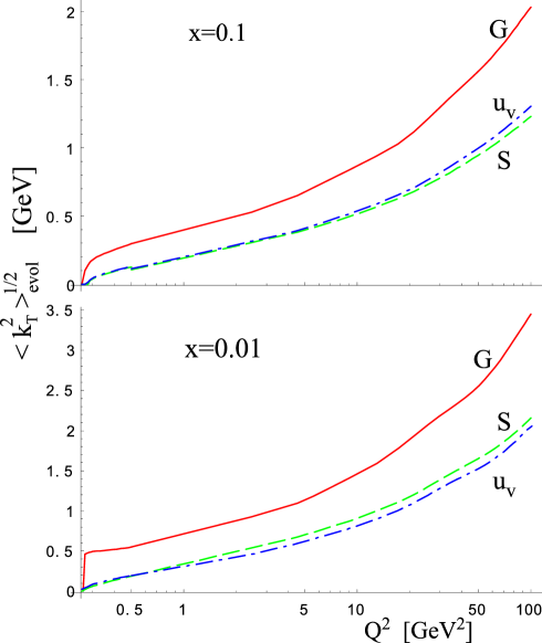
Figure 5: Same as Fig. 4 for the case of the nucleon, with the initial GRV parameterisation [35].

Figure 6: Same as Fig. 3 for the case of the nucleon, with the initial GRV parameterisation [35].

4 Evolution of the $x$-moments

The evolution equation for the $x$-moments of the non-singlet distribution,

$$\tilde{f}_{\rm NS}(n,b,Q^{2})=\int_{0}^{1}dx\,x^{n-1}\tilde{f}_{\rm NS}(x,b,Q),$$ (34)

is particularly simple. It immediately follows from Eq. (18) that

$$Q^{2}\frac{\partial\tilde{f}_{\rm NS}(n,b,Q^{2})}{\partial Q^{2}}=\frac{\alpha_{S}(Q^{2})}{2\pi}\int_{0}^{1}dzP_{qq}(z)\left[z^{n}J_{0}\left((1-z)Qb)\right)-1\right]\,\tilde{f}_{\rm NS}(n,b,Q),$$

(35)

which can be transformed into

$$Q^{2}\frac{\partial\log\left(\tilde{f}_{\rm NS}(n,b,Q^{2})\right)}{\partial Q^{2}}=\frac{\alpha_{S}(Q^{2})}{2\pi}\int_{0}^{1}dz\frac{4}{3}\frac{z^{2}+1}{1-z}\left[z^{n}J_{0}\left((1-z)Qb)\right)-1\right].$$ (36)

At $b=0$ this equation reproduces the standard evolution of non-singlet moments for the DGLAP equations. Next, we differentiate with respect to $b^{2}$ at $b=0$ on both sides of Eq. (36) and evaluate the $z$ integral on the right-hand side. The simple result is

$$\frac{\partial\langle k^{2}_{T}(n,Q^{2})\rangle_{\rm NS,evol}}{\partial Q^{2}}=\frac{\alpha_{S}(Q^{2})}{2\pi}c_{n},$$ (37)

with the definition

$$\langle k^{2}_{T}(n,Q^{2})\rangle_{\rm NS,evol}=\frac{\int d^{2}{\bf k}_{T}\,k_{T}^{2}\tilde{f}_{\rm NS}(n,k_{T},Q)}{\int d^{2}{\bf k}_{T}\,\tilde{f}_{\rm NS}(n,k_{T},Q}$$ (38)

and

$$c_{n}=\frac{4}{3}\left(\frac{1}{n+1}-\frac{1}{n+2}+\frac{1}{n+3}-\frac{1}{n+4}\right).$$ (39)

The integration of Eq. (37) with the condition $\langle k^{2}_{T}(n,Q_{0}^{2})\rangle_{\rm NS,evol}(Q_{0}^{2})=0$ yields the final result

$$\langle k^{2}_{T}(n,Q^{2})\rangle_{\rm NS,evol}=c_{n}\int_{Q^{2}_{0}}^{Q^{2}}dq^{2}{\alpha_{s}(q^{2})\over 2\pi},$$ (40)

where

$$\int_{Q^{2}_{0}}^{Q^{2}}dq^{2}{\alpha_{s}(q^{2})\over 2\pi}=\frac{2\Lambda_{QCD}^{2}}{\beta_{0}}\left[{\rm li}\left(\frac{Q^{2}}{\Lambda_{QCD}^{2}}\right)-{\rm li}\left(\frac{Q_{0}^{2}}{\Lambda_{QCD}^{2}}\right),\right]$$ (41)

with $\beta_{0}=11N_{c}/9-2N_{f}/3$ and ${\rm li}(z)=\int_{0}^{z}dt/\log t$. Obviously, the moments for all values of $n$ are growing with $Q^{2}$, which once again is a manifestation of the advocated spreading in $k_{T}$.

The analysis for the gluon and singlet quarks is more complicated due to mixing and is discussed in the Appendix. The evolution parts $<k^{2}_{T}(n,Q^{2})>_{\rm i,evol}$, with $i={\rm G,S}$, are equal to

$$<k^{2}_{T}(n,Q^{2})>_{\rm i,evol}=-4{f_{\rm i,evol}^{\prime}(n,Q^{2})\over f_{\rm i,evol}(n,Q^{2})},$$ (42)

with the functions $f_{i,evol}^{\prime}(n,Q^{2})$ and $f_{i,evol}(n,Q^{2})$ defined in Eqs. (58) and (72) in the Appendix. From those formulas and from equation (40) it follows that $<k^{2}_{T}(n,Q^{2})>_{\rm i}$ increases as $Q^{2}$, modulo logarithmic effects. This increase is caused by the fact that $-f_{\rm i,evol}^{\prime}(n,Q^{2})$ is found to increase as $Q^{2}$ modulo logarithmic effects caused by QCD scaling violations. Similar strong increase should also hold for $-d/db^{2}\tilde{f}_{i}(b,x,Q)|_{b=0}$ controlling $Q^{2}$ dependence of $<k_{T}^{2}(x,Q^{2})>_{i,evol}$

The results for the dynamically-generated root mean squared transverse momentum for the $x$ moments of the distributions in the pion, $<k^{2}_{T}(n,Q^{2})>_{\rm i,evol}$, are shown in Fig. 7. For $n=0$ only the nonsinglet distribution is shown, since the gluon and singlet equations involve singularities and do not make sense in this case. The solid, dashed, and dot-dashed lines denote gluons, singlet quarks, and non-singlet quarks. Again we use the initial GRS condition [34] at the scale $Q^{2}=Q_{0}^{2}=0.26~{}{\rm GeV}^{2}$. The analogous plot for the nucleon with the GRV parameterisation [35] gives identical results for the nonsinglet distributions, which follows immediately from Eq. (38) not involving the initial values of the moments. For the gluons and singlet quarks the results for the pion and the nucleon, although not strictly equal (see the Appendix), are practically identical. The results displayed in Fig. 7 once again show the main observation of this paper, namely, a large spreading of the distributions in process of the single-loop CCFM evolution.

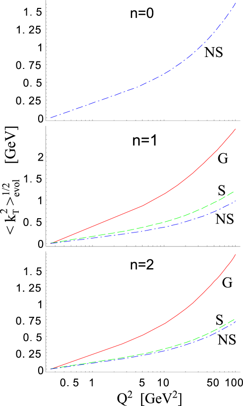
Figure 7: The dynamically-generated root mean squared transverse momentum of unintegrated partonic distribution functions in the pion corresponding to the $x$ moments of the distributions, plotted as a function of $Q^{2}$ for the moment index $n=0$ (top), $n=1$ (middle), and $n=2$ (bottom). The solid, dashed, and dot-dashed lines denote gluons, singlet quarks, and non-singlet quarks. For $n=0$ only the non-singlet distribution makes sense. The CCFM equations in the single-loop approximation with the initial GRS condition [34] at the scale $Q^{2}=Q_{0}^{2}=0.26~{}{\rm GeV}^{2}$ are used for the evolution. The analogous plot for the nucleon with the GRV parameterisation gives identical results for the nonsinglet distributions, and practically identical for the gluons and singlet quarks.

5 Parton-parton luminosity function

The knowledge of unintegrated distributions in the $b$ representation is useful for calculations of the parton-parton luminosity function corresponding to the collision of parton $a$ with the longitudinal momentum fraction $x_{1}$ and the transverse momentum fraction $k_{1T}$ with parton $b$ with the longitudinal momentum fraction $x_{2}$ and the transverse momentum fraction $k_{2T}$. The luminosity function is defined as [3]:

$$L_{ab}(x_{1},x_{2},q_{T},Q)=\int\frac{d^{2}{\bf k_{1T}}d^{2}{\bf k_{2T}}}{\pi}f_{a}(x_{1},k_{1T},Q)f_{b}(x_{2},k_{2T},Q)\delta^{(2)}({\bf k_{1T}}+{\bf k_{2T}}-{\bf q_{T}}).$$ (43)

Substituting in Eq. (43) the following representation of the $\delta$ function,

$$\delta^{(2)}({\bf k_{1T}}+{\bf k_{2T}}-{\bf q_{T}})={1\over(2\pi)^{2}}\int d^{2}{\bf b}\exp[({\bf k_{1T}}+{\bf k_{2T}}-{\bf q_{T}}){\bf b}],$$ (44)

we find that the integral defining the parton-parton luminosity in Eqn. (43) can be directly expressed in terms of the unintegrated distributions in the $b$ representation,

$$L_{ab}(x_{1},x_{2},q_{T},Q)=\int_{0}^{\infty}db^{2}f_{a}(x_{1},b,Q)f_{b}(x_{2},b,Q)J_{0}(bq_{T}).$$ (45)

In Fig. 8 we show the luminosity function corresponding to the valence $u$ quark-gluon collisions. This quantity is relevant for the description of prompt photon production for which the dominant subprocess is $u+g\rightarrow u+\gamma$. We set $Q=p_{\gamma T}$ and $x_{1}=x_{2}={2p_{\gamma T}}/{\sqrt{s}}$ where $\sqrt{s}$ is the CM energy of the $p\bar{p}$ collisions. The two curves correspond to $\sqrt{s}=24.3{\rm GeV}$, $p_{\gamma T}=4{\rm GeV}$ and $\sqrt{s}=1800{\rm GeV}$, $p_{\gamma T}=10{\rm GeV}$. We can see that the luminosity function is increasing with the energy, which simply reflects the increase of the unintegrated gluon distributions with decreasing $x={2p_{\gamma T}}/{\sqrt{s}}$.

Figure 8: The parton luminosity function corresponding to the valence $u$ quark - gluon collisions plotted as the function of the transverse momentum $q_{T}$ equal to the vector sum of the transverse momenta of the colliding partons. The value of the hard scale $Q$ is set to the transverse momentum $p_{\gamma T}$ of the produced photon. The two curves correspond to two values of the total $\bar{p}p$ CM energy $\sqrt{s}$ and different values of $p_{\gamma T}$: $\sqrt{s}=24.3{\rm GeV}$, $p_{\gamma T}=4{\rm GeV}$ (dashed line) and $\sqrt{s}=1800{\rm GeV}$, $p_{\gamma T}=10{\rm GeV}$ (full line). Results for $\sqrt{s}=24.3{\rm GeV}$ were multiplied by $10$. The parton luminosity function $L$ is in ${\rm GeV^{-2}}$ and transverse momentum $q_{T}$ is in ${\rm GeV}$.

6 Summary and conclusions.

In this paper we have performed an analysis of the unintegrated parton distributions $f_{i}(x,k_{T},Q)$ of the pion and nucleon using the CCFM equation in the single loop approximation. For the integrated distributions this approximation is equivalent to the LO DGLAP evolution, and thus should be adequate in the region of large and moderately small values of $x$ (i.e. $x>0.01$ or so). Important merit of the CCFM framework is the fact that once the input $x$ and $k_{T}$ parton distributions are provided at the reference scale $Q_{0}^{2}$, the CCFM evolution generates the $x$ and $k_{T}$ distributions for arbitrary $Q^{2}>Q_{0}^{2}$ and arbitrary values of $k_{T}$, including the region of low $k_{T}$ down to the point $k_{T}=0$. This framework does therefore provide a useful extension of the approximate DGLAP - based treatment of the unintegrated distributions discussed in [2, 3]. We have extended the original CCFM equation by including the quarks and non-singular parts of the splitting functions and used the transverse-coordinate representation by introducing the parton distribution $\bar{f}_{i}(x,b,Q)$, related to the unintegrated parton distributions $f_{i}(x,k_{T},Q)$ through the Fourier-Bessel transform. The usefulness of this representation is related to the fact that the transverse coordinate $b$ is conserved through the CCFM evolution in the single loop approximation. The average transverse momenta squared of the partons are determined by $d\bar{f}_{i}(x,b,Q)/db^{2}|_{b=0}$. We have studied the impact of the QCD evolution on the shape of the $b$ profiles and on the broadening of the $k_{T}$ distributions. We have quantified increase of the average transverse momentum with increasing magnitude of the hard scale $Q$ and/or with decreasing $x$ and we gave semianalytic insight into this increase. The average transverse momenta squared of the partons were found to increase as $Q^{2}$ with increasing $Q^{2}$, modulo logarithmic effects related to the QCD evolution. We have also pointed out that the parton distributions in $b$ representation determine the parton luminosity functions for fixed sum of the transverse momenta of the partons. The unintegrated distributions $f_{i}(x,k_{T},Q)$ (or $f_{i}(x,b,Q)$) obtained in our paper can be used for the theoretical description of the processes which are sensitive to the transverse momenta of the partons.

Appendix

The average value of the transverse momentum $<k_{T}^{2}(n)>_{i}$ is given by

$$<k_{T}^{2}(n,Q^{2})>_{i}=-4{f_{i}^{\prime}(n,Q^{2})\over f_{i}(n,Q^{2})}$$ (46)

where

$$f_{i}^{\prime}(n,Q^{2}) = {df_{i}(n,b^{2},Q^{2})\over db^{2}}|_{b^{2}=0},$$

$$f_{i}(n,Q^{2}) = f_{i}(n,b^{2}=0,Q^{2}),$$ (47)

and $f_{i}(n,b^{2},Q^{2})$ are the moment functions,

$$f_{i}(n,b^{2},Q^{2})=\int_{0}^{1}dxx^{n-1}\bar{f}_{i}(x,b,Q).$$ (48)

The index $i$ corresponds to the gluon, quark singlet, or quark non-singlet distributions. In the case of the quark NS distributions we just have

$$<k_{T}^{2}(n,Q^{2})>_{\rm NS} = <k_{T}^{2}(n,Q_{0}^{2})>_{\rm NS}+\int_{0}^{1}dzz^{n}(1-z)^{2}P_{qq}(z)\int_{Q_{0}^{2}}^{Q^{2}}dq^{2}{\alpha_{s}(q^{2})\over 2\pi}$$ (49)

$$= <k_{T}^{2}(n,Q_{0}^{2})>_{\rm NS}+<k_{T}^{2}(n,Q_{0}^{2})>_{\rm NS,evol}$$

In what follows we derive analytic expression for the dynamical component $<k_{T}^{2}(n,Q^{2})>_{i,{\rm evol}}$ of $<k_{T}^{2}(n,Q^{2})>_{i}$ corresponding to the gluon and quark singlet distributions. To this aim we start from the system of the evolution equations:

$$Q^{2}{d\hat{f}^{\prime}(n,Q^{2})\over dQ^{2}}={\alpha_{s}(Q^{2})\over 2\pi}\left[\hat{P}(n)\hat{f}^{\prime}(n,Q^{2})-{Q^{2}\over 4}\hat{P}^{\prime}(n)\hat{f}(n,Q^{2})\right],$$ (50)

obtained from Eqs. (…) by differentiation with respect to $b^{2}$. The components of the vector $\hat{f}^{\prime}(n,Q^{2})$ are $f_{S}^{\prime}(n,Q^{2})$ and $f_{G}^{\prime}(n,Q^{2})$, while the components of the matrices $\hat{P}(n)$ are equal to the moments of the splitting functions defining DGLAP evolution of the moments of singlet and gluon distributions, namely,

$$\hat{P}_{qq}(n) = \int_{0}^{1}dzP_{qq}(z)[z^{n}-1],$$

$$\hat{P}_{gg}(n) = \int_{0}^{1}dz\{zP_{gg}(z)[z^{n-1}-1]-zP_{qg}\},$$

$$\hat{P}_{qg,gq}(n) = \int_{0}^{1}dzP_{qg,gq}(z)z^{n}.$$ (51)

The explicit expressions for the functions $\hat{P}_{ij}(n)$ are

$$\hat{P}_{qq}(n) = {4\over 3}\left[{3\over 2}-{1\over n+1}-{1\over n+2}-2S(n)\right],$$

$$\hat{P}_{qg}(n) = N_{f}\left[{1\over n+1}-{2\over n+2}+{2\over n+3}\right],$$

$$\hat{P}_{gq}(n) = {4\over 3}\left[{2\over n}-{2\over n+1}+{1\over n+2}\right],$$

$$\hat{P}_{gq}(n) = 6\left[{11\over 12}-S(n)+{1\over n}-{2\over n+1}+{1\over n+2}-{1\over n+3}\right]-{N_{f}\over 3},$$ (52)

where

$$S(n)=\int_{0}^{1}dz{1-z^{n}\over 1-z}=\sum_{k=1}^{n}\frac{1}{k}.$$ (53)

Similarly, the components of the matrices $\hat{P}^{\prime}(n)$ are defined as

$$\hat{P}_{ab}^{\prime}(n)=\int_{0}^{1}dz(1-z)^{2}P_{ab}(z)z^{n},$$ (54)

with the explicit expressions given by

$$\hat{P}_{qq}^{\prime}(n) = {4\over 3}\left[{1\over n+1}-{1\over n+2}+{1\over n+3}-{1\over n+4}\right],$$

$$\hat{P}_{qg}^{\prime}(n) = N_{f}\left[{1\over n+1}-{4\over n+2}+{7\over n+3}-{6\over n+4}+{2\over n+5}\right],$$

$$\hat{P}_{gq}^{\prime}(n) = {4\over 3}\left[{2\over n}-{6\over n+1}+{7\over n+2}-{4\over n+3}+{1\over n+4}\right],$$

$$\hat{P}_{gg}^{\prime}(n) = 6\left[{1\over n}-{3\over n+1}+{5\over n+2}-{5\over n+3}+{3\over n+4}-{1\over n+5}\right].$$ (55)

The dynamical components $<k_{T}^{2}(n,Q^{2})>_{i,{\rm evol}}$ of $<k_{T}^{2}(n,Q^{2})>_{i}$ are given by Eq. (46) with $f^{\prime}_{i}(n,Q^{2})=f^{\prime}_{i,evol}(n,Q^{2})$ corresponding to the solution of Eq. (50) with the initial condition $f^{\prime}_{i}(n,Q_{0}^{2})=0$. The solution of Eq. (50) with the initial condition $\hat{f}^{\prime}(n,Q^{2}=Q_{0}^{2})=0$ can be formally written as

$$\hat{f}^{\prime}_{evol}(n,Q^{2})=-{1\over 4}\int_{Q_{0}^{2}}^{Q^{2}}dq^{2}{\alpha_{s}(q^{2})\over 2\pi}\exp\{\hat{P}(n)[\xi(Q^{2})-\xi(q^{2})]\}\hat{P}^{\prime}(n)\hat{f}(n,q^{2}),$$ (56)

where

$$\xi(q^{2})=\int_{Q_{0}^{2}}^{q^{2}}{dq^{\prime 2}\over q^{\prime 2}}{\alpha_{s}(q^{\prime 2})\over 2\pi}.$$ (57)

This representation gives, after some algebra, the following explicit expressions for $f^{\prime}_{\rm S,evol}(n,Q^{2})$ and $f^{\prime}_{\rm G,evol}(n,Q^{2})$:

$$f^{\prime}_{S,G,evol}(n,Q^{2})=$$

$$-{1\over 4}\{\exp[\gamma^{+}(n)\xi(Q^{2})][h_{S,G}^{++}(n)\eta(0,Q^{2})+h_{S,G}^{+-}(n)\eta(-\sqrt{\Delta(n)},Q^{2})]$$

$$+\exp[\gamma^{-}(n)\xi(Q^{2})][h_{S,G}^{--}(n)\eta(0,Q^{2})+h_{S,G}^{+-}(n)\eta(\sqrt{\Delta(n)},Q^{2})]\},$$ (58)

where

$$\eta(r,Q^{2})=\int_{Q_{0}^{2}}^{Q^{2}}dq^{2}{\alpha_{s}(q^{2})\over 2\pi}\exp[r\xi(q^{2})]$$ (59)

The functions $\gamma^{mp}(n)$ are the eigenvalues of of the matrix $\hat{P}(n)$ and are given by

$$\gamma^{\mp}(n)={P_{qq}(n)+P_{gg}(n)\mp\sqrt{\Delta(n)}\over 2},$$ (60)

with

$$\Delta(n)=[P_{qq}(n)-P_{gg}(n)]^{2}+4P_{qg}(n)P_{gq}(n).$$ (61)

The coefficients $h^{++}_{S,G}(n)$, $h^{+-}_{S,G}(n),h^{--}_{S,G}(n)$, and $h^{-+}_{S,G}(n)$ are expressed in terms of the input moments $f_{S,G}(n,Q_{0}^{2})$

$$h^{++}_{S}(n) = {1\over\sqrt{\Delta(n)}}\{[\gamma^{+}(n)-P_{gg}(n)][P^{\prime}_{qq}(n)f_{S}^{+}(n,Q_{0}^{2})+P^{\prime}_{qg}(n)f_{G}^{+}(n,Q_{0}^{2})]$$ (62)

$$+ P_{qg}(n)[P^{\prime}_{gq}(n)f_{S}^{+}(n,Q_{0}^{2})+P^{\prime}_{gg}(n)f_{G}^{+}(n,Q_{0}^{2})]\}$$

$$h^{++}_{G}(n) = {1\over\sqrt{\Delta(n)}}\{P_{gq}(n)[P^{\prime}_{qq}(n)f_{S}^{+}(n,Q_{0}^{2})+P^{\prime}_{qg}(n)f_{G}^{+}(n,Q_{0}^{2})]$$ (63)

$$+ [\gamma^{+}(n)-P_{qq}(n)][P^{\prime}_{gq}(n)f_{S}^{+}(n,Q_{0}^{2})+P^{\prime}_{gg}(n)f_{G}^{+}(n,Q_{0}^{2})]\}$$

$$h^{+-}_{S}(n) = {1\over\sqrt{\Delta(n)}}\{[\gamma^{+}(n)-P_{gg}(n)][P^{\prime}_{qq}(n)f_{S}^{-}(n,Q_{0}^{2})+P^{\prime}_{qg}(n)f_{G}^{-}(n,Q_{0}^{2})]$$ (64)

$$+ P_{qg}(n)[P^{\prime}_{gq}(n)f_{S}^{-}(n,Q_{0}^{2})+P^{\prime}_{gg}(n)f_{G}^{-}(n,Q_{0}^{2})]\}$$

$$h^{+-}_{G}(n) = {1\over\sqrt{\Delta(n)}}\{P_{gq}(n)[P^{\prime}_{qq}(n)f_{S}^{-}(n,Q_{0}^{2})+P^{\prime}_{qg}(n)f_{G}^{-}(n,Q_{0}^{2})]$$ (65)

$$+ [\gamma^{+}(n)-P_{qq}(n)][P^{\prime}_{gq}(n)f_{S}^{-}(n,Q_{0}^{2})+P^{\prime}_{gg}(n)f_{G}^{-}(n,Q_{0}^{2})]\}$$

$$h^{--}_{S}(n) = -{1\over\sqrt{\Delta(n)}}\{[\gamma^{-}(n)-P_{gg}(n)][P^{\prime}_{qq}(n)f_{S}^{-}(n,Q_{0}^{2})+P^{\prime}_{qg}(n)f_{G}^{-}(n,Q_{0}^{2})]$$ (66)

$$+ P_{qg}(n)[P^{\prime}_{gq}(n)f_{S}^{-}(n,Q_{0}^{2})+P^{\prime}_{gg}(n)f_{G}^{-}(n,Q_{0}^{2})]\}$$

$$h^{--}_{G}(n) = -{1\over\sqrt{\Delta(n)}}\{P_{gq}(n)[P^{\prime}_{qq}(n)f_{S}^{-}(n,Q_{0}^{2})+P^{\prime}_{qg}(n)f_{G}^{-}(n,Q_{0}^{2})]$$ (67)

$$+ [\gamma^{-}(n)-P_{qq}(n)][P^{\prime}_{gq}(n)f_{S}^{-}(n,Q_{0}^{2})+P^{\prime}_{gg}(n)f_{G}^{-}(n,Q_{0}^{2})]\}$$

$$h^{-+}_{S}(n) = -{1\over\sqrt{\Delta(n)}}\{[\gamma^{-}(n)-P_{gg}(n)][P^{\prime}_{qq}(n)f_{S}^{+}(n,Q_{0}^{2})+P^{\prime}_{qg}(n)f_{G}^{+}(n,Q_{0}^{2})]$$ (68)

$$+ P_{qg}(n)[P^{\prime}_{gq}(n)f_{S}^{+}(n,Q_{0}^{2})+P^{\prime}_{gg}(n)f_{G}^{+}(n,Q_{0}^{2})]\}$$

$$h^{-+}_{G}(n) = -{1\over\sqrt{\Delta(n)}}\{P_{gq}(n)[P^{\prime}_{qq}(n)f_{S}^{+}(n,Q_{0}^{2})+P^{\prime}_{qg}(n)f_{G}^{+}(n,Q_{0}^{2})]$$ (69)

$$+ [\gamma^{-}(n)-P_{qq}(n)][P^{\prime}_{gq}(n)f_{S}^{+}(n,Q_{0}^{2})+P^{\prime}_{gg}(n)f_{G}^{+}(n,Q_{0}^{2})]\},$$

where

$$f_{S}^{\mp}(n,Q_{0}^{2}) = \mp{1\over\sqrt{\Delta}}\{[\gamma^{\mp}(n)-P_{gg}]f_{S}(n,Q_{0}^{2})+P_{qg}(n)f_{G}(n,Q_{0}^{2})\},$$ (70)

$$f_{G}^{\mp}(n,Q_{0}^{2}) = \mp{1\over\sqrt{\Delta}}\{[\gamma^{\mp}(n)-P_{qq}]f_{G}(n,Q_{0}^{2})+P_{gq}(n)f_{S}(n,Q_{0}^{2})\}.$$ (71)

The functions $f_{S,G}(n,Q^{2})$ are given by:

$$f_{S,G}(n,Q^{2})=f_{S,G}^{+}(n,Q_{0}^{2})\exp[\gamma^{+}(n)\xi(Q^{2})]+f_{S,G}^{-}(n,Q_{0}^{2})exp[\gamma^{-}(n)\xi(Q^{2})]$$ (72)

References

- [1] R.K. Ellis, W.J. Stirling, B.R. Webber, ’QCD and Collider Physics’, Cambridge University Press, 1996.
- [2] Yu.L. Dokshitzer, D.I. Dyakonov and S.I. Troyan, Phys. Rep. 58 (1980) 269.
- [3] M.A. Kimber, A.D.Martin and M.G. Ryskin, Eur. Phys. J. C12 (2000) 655.
- [4] M.A. Kimber, A.D.Martin, J. Kwieciński and A.M. Staśto, Phys. Rev. D62 (2000) 094006.
- [5] M.A. Kimber, A.D.Martin and M.G. Ryskin, Phys. Rev. D63 (2001) 114027.
- [6] A.D. Martin and M.G.Ryskin, Phys. Rev. D64 (2001) 094017.
- [7] V.A. Khoze, A.D. Martin and M.G. Ryskin, Eur. Phys. J. C14 (2000) 525; ibid. C19 (2001) 477; Erratum - ibid. C20 (2001) 599.
- [8] G. Gustafson, L. Lönnblad and G. Miu, JHEP 0209 (2002)005.
- [9] A. Szczurek, hep-ph/0304129.
- [10] Small Collaboration (B. Andersson et al.), Eur. Phys. J. C25 (2002) 77.
- [11] J.C. Collins, hep-ph/0304122.
- [12] S. Catani, M. Ciafaloni and F. Hautmann, Phys. Lett. B242 (1990) 97; Nucl. Phys. B366 (1991) 657; S. Catani and F. Hautmann, Nucl. Phys. B427 (1994) 475; J.C. Collins and R.K. Ellis, Nucl. Phys. B360 (1991) 3.
- [13] A. Szczurek, Eur. Phys. J. C26 (2002) 183.
- [14] L. Motyka, N. Timneanu, Eur. Phys. J. C26 (2002) 183.
- [15] A.V. Kotikov, A.V. Lipatov, N.P. Zotov, Eur. Phys. J. C27 (2003) 219; A.V. Lipatov, N.P. Zotov, hep-ph/0304181; Eur. Phys. J. C27 (2003) 87; A.V. Lipatov, V.A. Saleev, N.P. Zotov, Mod. Phys. Lett. A15 (2000) 1727.
- [16] I.P. Ivanov, hep-ph/0303053; Acta Phys. Polon. B33 (2002) 3517; I.P. Ivanov, N.N. Nikolaev, Phys. Rev. D65 (2002) 054004.
- [17] M. Ciafaloni, Nucl. Phys. B296 (1988) 49; S. Catani, F. Fiorani and G. Marchesini, Phys. Lett. B234 (1990) 339; Nucl. Phys. B336 (1990) 18.
- [18] G. Marchesini, in Proceedings of the Workshop ”QCD at 200 TeV”, Erice, Italy, 1990, edited by L. Cifarelli and Yu. L. Dokshitzer, (Plenum Press, New York, 1992), p. 183.
- [19] B.R. Webber Nucl. Phys. B (Proc. Suppl.) 18C (1990) 38.
- [20] G.Marchesini and B.R. Webber, Nucl. Phys. B386 (1992) 215; B.R. Webber in Proceedings of the Workshop ”Physics at HERA”, DESY, Hamburg, Germany, 1992, edited by W. Buchmüller and G. Ingelman (DESY, Hamburg, 1992).
- [21] G. Marchesini, Nucl.Phys. B445 (1995) 49.
- [22] J. Kwieciński, A.D. Martin and P.J. Sutton, Phys. Rev. D52 (1995) 1445.
- [23] G. Bottazzi, G. Marchesini, G.P. Salam and M Scorletti, Nucl. Phys. B505 (1997) 366; JHEP 9812 (2998) 011.
- [24] K. Golec-Biernat, L. Goerlich and J. Turnau, Nucl. Phys. B527 (1998) 289.
- [25] G.P. Salam, JHEP 9903 (1999) 009; Nucl. Phys.Proc. Suppl. 79 (1999) 426.
- [26] H. Jung, Nucl. Phys. Proc. Suppl. 79 (1999) 429; Phys. Rev. D65 (2002) 034015; Comput. Phys. Commun. 143 (2002) 100; J. Phys. G28 (2002) 971.
- [27] H. Jung and G.P. Salam, Eur. Phys. J. C19 (2001) 351.
- [28] Yu.L. Dokshitzer, V.A. Khoze, S.I. Troyan and A.H. Mueller, Rev. Mod. Phys. 60 (1988) 373.
- [29] A. Bassetto, M. Ciafaloni, G. Marchesini, Nucl. Phys. B163 (1980) 429.
- [30] J. Kodaira, L. Trentadue, Phys. Lett. B112 (1982) 66.
- [31] Y.I.Dokshitzer, D.I.Dyakonov and S.I.Troyan, Phys. Lett. B79 (1978) 269; G. Parisi and R.Petronzio, Nucl. Phys. B154 (1979) 427; J. Collins and D. Soper, Phys. Rev. D16 (1977) 2219; J. Collins, D. Soper, G. Sterman, Nucl. Phys. B250 (1985) 199; G. Altarelli, R.K. Ellis, M. Greco and G. Martinelli, Nucl. Phys. B246 (1984) 12; C.T.H. Davies and W.J. Stirling, Nucl. Phys. B244 (1984) 337; C.T.H. Davies, B.R. Webber, W.J. Stirling, Nucl. Phys. B256 (1985) 413; J.W. Qiu and X.F. Zhang, Phys. Rev. D63 (2001) 114011.
- [32] J. Kwieciński, Acta Phys. Polon. B33 (2002) 1809.
- [33] A. Gawron, J. Kwieciński, Acta Phys. Polon. B34 (2003) 133.
- [34] M. Glück, E. Reya, I. Schienbein, Eur. Phys. J. C10 (1999) 313.
- [35] M. Glück, E. Reya, A. Vogt, Eur. Phys. J. C5 (1998) 461.
- [36] J. Kwiecinski, D. Strozik-Kotlorz, Z. Phys. C48 (1990) 315.