Quantum dynamics of $\Phi^{4}$ field theory beyond leading order in $1+1$ dimensions

Abstract

We consider the out-of-equilibrium evolution of a classical condensate field $\phi=\left<\Phi\right>$ and its quantum fluctuations for a $\Phi^{4}$ model in $1+1$ dimensions with a double well potential. We use the two-particle point-irreducible (2PPI) formalism in the two-loop approximation. We compare our results to those obtained in the Hartree approximation, in the bare vertex approximation (BVA) and in the two-particle irreducible next-to-leading order large-N (2PI-1/N) approach, with thermal initial conditions. In the 2PPI scheme we find that the system tends to the symmetric configuration at late times, as expected in the absence of spontaneous symmetry breaking.

I Introduction

In recent years there was considerable activity in extending the study of quantum field theory out of equilibrium beyond the leading order one-loop, large-$N$ and Hartree approximations Berges:2000ur ; Berges:2001fi ; Blagoev:2001ze ; Aarts:2002dj ; Cooper:2002ze ; Berges:2002cz ; Cooper:2002qd ; Baacke:2002ee .

The simple $\Phi^{4}$ quantum field theory serves as a toy model for more realistic models with more degrees of freedom. Such models are e.g. candidates for a description of the inflationary phase of the early universe.

Recent numerical simulations Cooper:2002qd ; Baacke:2002ee ; Mihaila:2003mh within different approximation schemes beyond leading order have lead to contradictory results for the phase structure of O(1) and O($N$) $\Phi^{4}$ models in $1+1$ dimensions. From finite temperature field theory it is known Griffiths , that in $1+1$ dimensions there should be no spontaneous symmetry breaking except at zero temperature; hence the absence of spontaneous symmetry breaking is expected in nonequilibrium quantum field theory as well. While the Hartree approximation gives a first order phase transition, the situation is different for various next-to-leading order approximation schemes.

Cooper et al. Cooper:2002qd have studied in detail the symmetry structure of the O(1) model in $1+1$ dimensions and the equilibration of the one- and two point correlation functions within the bare vertex approximation (BVA) and the two-particle irreducible next-to-leading order large-N (2PI-1/N) scheme. They found a second-order phase transition in the BVA and no spontaneous symmetry breaking in the 2PI-1/N approximation. Both approximation schemes are based on the so called Cornwall-Jackiw-Tomboulis (CJT) effective action Cornwall:1974vz . In the CJT formalism the effective action is expanded in terms of two-particle irreducible (2PI) diagrams. The self energy fulfills a Schwinger-Dyson equation and resums this 2PI diagrams. A related approximation proposed by Verschelde and Coppens Verschelde:1992bs ; Coppens:1993zc is the two-particle point-irreducible (2PPI) formalism, where only local contributions to the self energy are considered. The one-loop 2PPI approximation represents the Hartree approximation. We have studied, in Ref. Baacke:2002ee , the $O(1)$ model within the two-loop 2PPI approximation and, with the parameters and initial conditions chosen there, we found no spontaneous symmetry breaking. In order to have a direct comparison with the results of Cooper et al. we present here numerical simulations using their parameters and initial conditions. Besides the question of spontaneous symmetry breaking it is interesting to compare the general features in the temporal evolution of all three approaches.

The plan of this paper is as follows: In section II we briefly summarize the model formulated in Baacke:2002ee and its extension to the case of an additional thermal initial state of quanta. In section III we present the results of the numerical calculations. We end with some conclusions in section IV.

II The model

The Lagrange density for the $\Phi^{4}$ quantum field theory is defined by

$${\cal L}=\frac{1}{2}\partial_{\mu}\Phi\partial^{\mu}\Phi-\frac{1}{2}\mu^{2}\Phi^{2}-\frac{\lambda}{4!}\Phi^{4}\ .$$ (2.1)

Here we will consider the case of a double well potential with $\mu^{2}<0$. Within the 2PPI formalism the inverse Green’s function $G^{-1}(x,x^{\prime})=i[\Box+{\cal M}^{2}(x)]\delta(x-x^{\prime})$ remains local and is parametrized by a variational mass ${\cal M}^{2}(t)$. The 2PPI effective action in terms of the variational parameters $\phi(t)$ and ${\cal M}^{2}(t)$ denotes Baacke:2002ee

$$\Gamma[\phi,{\cal M}^{2}] = \int d^{2}x\left[\frac{1}{2}\partial_{\mu}\phi(x)\,\partial^{\mu}\phi(x)-\frac{1}{2}{\cal M}^{2}(x)\phi^{2}(x)\right.$$ (2.2)

$$\hskip 28.45274pt+\left.\frac{\lambda}{12}\phi^{4}(x)+\frac{1}{2\lambda}\left({\cal M}^{2}(x)-\mu^{2}\right)^{2}\right]$$

$$+\Gamma^{\rm 2PPI}[\phi,{\cal M}^{2}]\;.$$

The term $\Gamma^{\mathrm{2PPI}}[\phi,{\cal M}^{2}]$ contains all 2PPI vacuum diagrams, i.e. all graphs that do not decay if two lines meeting at the same point are cut.

By variation of the effective action $\Gamma[\phi,{\cal M}^{2}]$ with respect to ${\cal M}^{2}$ one easily checks that ${\cal M}^{2}(x)$ satisfies the gap or Schwinger-Dyson equation

$${\cal M}^{2}(x)=\mu^{2}+\frac{\lambda}{2}\phi^{2}(x)+\frac{\lambda}{2}\Delta(x)\ ,$$ (2.3)

where the insertion $\Delta(x)$ has been defined as

$$\Delta(x)=-2\frac{\delta\Gamma^{\rm 2PPI}[\phi,{\cal M}^{2}]}{\delta{\cal M}^{2}(x)}\ .$$ (2.4)

This form of the effective action in terms of $\phi$ and ${\cal M}^{2}$ is analogous to the one with $\phi$ and $\Delta$ proposed by Verschelde and Coppens Verschelde:1992bs ; Coppens:1993zc .

By truncation of the infinite series of 2PPI graphs in $\Gamma^{\mathrm{2PPI}}$ one obtains an approximation for the effective action. The two graphs depicted in Fig. 1 represent the relevant contributions to $\Gamma^{\rm 2PPI}$ in the two-loop approximation, that will be used here. If only the one-loop bubble graph is included we refer to it as Hartree approximation.

(a)          (b)

Figure 1: We display the leading diagrams in the 2PPI action $\Gamma^{{\rm 2PPI}}$: (a) the bubble diagram; (b) the sunset diagram; solid lines: internal propagators; dashed lines: external fields $\phi$.

In the following we will consider only spatially homogeneous fields. Time integrations are understood to be carried out along a closed time path (CTP) Schwinger:1961qe ; Keldysh:1964ud ; Calzetta:1987ey .

The initial density matrix of the system is characterized by a nonzero value $\phi(0)$ for the mean field and a distribution function $n_{p}$ for the quanta. We will assume a Bose-Einstein distributed initial state of quanta parametrized by

$$n_{p}=\frac{1}{e^{\omega_{p}/T_{0}}-1}\$$ (2.5)

with $\omega_{p}=\sqrt{p^{2}+m_{0}^{2}}$, where $m_{0}^{2}$ is defined below. The Green’s function can therefore be written in terms of mode functions as

$$G(t,t^{\prime};p) = \frac{1}{2\omega_{p}}\left(2n_{p}+1\right)\left[f(t,p)f^{*}(t^{\prime},p)\Theta(t-t^{\prime})\right.$$ (2.6)

$$\qquad\left.+f(t^{\prime},p)f^{*}(t,p)\Theta(t^{\prime}-t)\right]\ .$$

The mode functions $f(t,p)$ satisfy the differential equation

$$\ddot{f}(t,p)+\left[p^{2}+{\cal M}^{2}(t)\right]f(t,p)=0\ .$$ (2.7)

The initial mass $m_{0}={\cal M}(0)$ has to be determined self consistently from the renormalized equation

$$m_{0}^{2}=\mu^{2}+\frac{\lambda}{2}\phi^{2}(0)+\delta\mu_{\mathrm{fin}}^{2}+\frac{\lambda}{2}\int\frac{dp}{2\pi}\frac{n_{p}}{\omega_{p}}\ ,$$ (2.8)

with $\delta\mu_{\mathrm{fin}}^{2}=\frac{\lambda}{8\pi}\ln\frac{\mu^{2}}{m_{0}^{2}}$. The mode functions at $t=0$ satisfy $f(0,p)=1$ and $\dot{f}(0,p)=-i\omega_{p}$.

The renormalized equations of motion in the two-loop approximation are

$$0 = \ddot{\phi}(t)+{\cal M}^{2}(t)\phi(t)-\frac{\lambda}{3}\phi^{3}(t)+{\cal S}(t)$$ (2.9)

$${\cal M}^{2}(t) = \mu^{2}+\delta\mu^{2}_{\mathrm{fin}}+\frac{\lambda}{2}\left(\phi^{2}(t)+\Delta^{(1)}_{\mathrm{fin}}(t)+\Delta^{(2)}(t)\right)$$

The finite one-loop part $\Delta^{(1)}_{\mathrm{fin}}$ has been defined as

$$\Delta^{(1)}_{\mathrm{fin}}(t)=\int\frac{dp}{2\pi 2\omega_{p}}\left[\left(2n_{p}+1\right)|f(t,p)|^{2}-1\right]\ .$$ (2.11)

The two-loop contributions are given by

$${\cal S}(t) = -i\frac{\lambda^{2}}{6}\int_{0}^{t}dt^{\prime}\phi(t^{\prime})$$ (2.12)

$$\times\int\prod_{\ell=1}^{3}\left(\frac{dp_{\ell}}{2\pi}\right)2\pi\delta\left(\sum_{\ell=1}^{3}p_{\ell}\right)$$

$$\times\left[\prod_{\ell=1}^{3}G(t,t^{\prime};p_{\ell})-\prod_{\ell=1}^{3}G(t^{\prime},t;p_{\ell})\right]\$$

and

$$\Delta^{(2)}(t) = -\lambda^{2}\int_{0}^{t}{dt^{\prime}}\phi(t^{\prime})\int_{0}^{t^{\prime}}{dt^{\prime\prime}}\phi(t^{\prime\prime})$$

$$\times\int\prod_{\ell=1}^{3}\left(\frac{dp_{\ell}}{2\pi}\right)2\pi\delta\left(\sum_{\ell=1}^{3}p_{\ell}\right)$$

$$\times\left[G(t,t^{\prime};p_{3})-G(t^{\prime},t;p_{3})\right]$$

$$\times\left[G(t^{\prime},t^{\prime\prime};p_{1})G(t^{\prime},t^{\prime\prime};p_{2})G(t,t^{\prime\prime};p_{3})\right.$$

$$\quad-\left.G(t^{\prime\prime},t^{\prime};p_{1})G(t^{\prime\prime},t^{\prime};p_{2})G(t^{\prime\prime},t;p_{3})\right]\;.$$

For the BVA and 2PI-1/N approximation Cooper et al. introduce the mass term $\chi(t)$ as an auxiliary field. Naively, in our scheme this corresponds to the quantity

$$\chi(t) = \mu^{2}+\delta\mu^{2}_{\mathrm{fin}}+\frac{\lambda}{2}\left[\phi^{2}(t)+\Delta^{(1)}_{\mathrm{fin}}(t)\right]$$ (2.14)

$$= {\cal M}^{2}(t)-\frac{\lambda}{2}\Delta^{(2)}(t)$$

where we have identified ${\rm Tr}G$ with $\Delta^{(1)}$. We note, however, that the Green’s functions have a different meaning in their and our schemes; this should be kept in consideration when comparing the numerical results.

III Results

The numerical implementation for the solution of the equations of motion [see Eq.(2.9) and (II)] has been described in detail in Ref. Baacke:2002ee . The equations of motion are solved using a Runge-Kutta algorithm with a time discretization $\Delta t=0.001$. The energy is conserved within five significant digits. We have chosen $\mu^{2}=-1$, $\phi(0)=0.4$, $T_{0}=0.1$ and $\lambda$ equal to $3.0$ and $21.3$. This choice of parameters corresponds to the one of Cooper et al. Cooper:2002qd .

The time evolution of the mean field $\phi(t)$ is presented in Fig. 2a and Fig. 3a and the time evolution of $\chi(t)$ is displayed in Fig. 2b and Fig. 3b. These are compared with the results obtained in the Hartree approximation, and to those obtained by Cooper et al. for the BVA and the 2PI-1/N approximations. For the simulation with $\lambda=21.3$ we additionally present the time evolution of the effective mass ${\cal M}^{2}(t)$ in Fig. 4 and the energy contributions in Fig. 5.

(a)

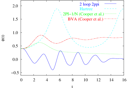
(b)

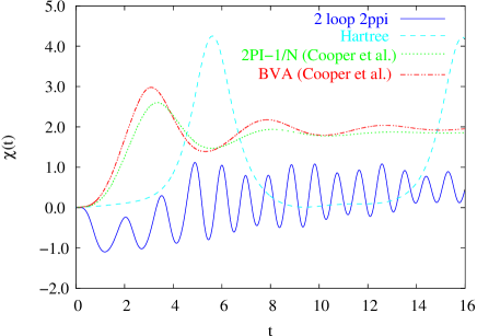
Figure 2: Time evolution for the double well potential. Parameters: $\mu^{2}=1$, $\lambda=3.0$, $\phi(0)=0.4$, $T_{0}=0.1$ (a) time evolution of the mean field $\phi(t)$; (b) time evolution of the field $\chi(t)$; the solid lines relate to the two-loop 2PPI approximation, the dashed lines to the one-loop 2PPI or Hartree approximation, the dotted lines to the 2PI-1/N approximation and the dashed dotted lines to the BVA approximation, where the last two simulations are taken from Cooper:2002qd

(a)

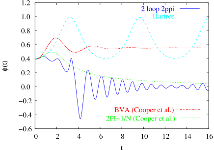
(b)

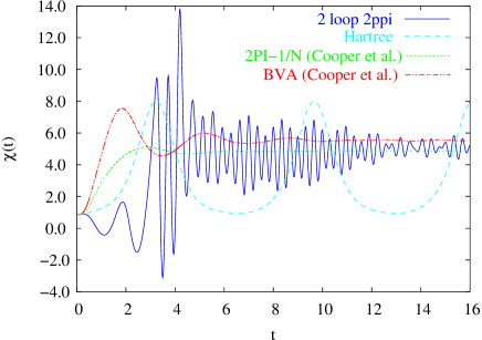
Figure 3: Same as Fig. 2 but for $\lambda=21.3$

Surprisingly the mean field obtained in the 2PPI approximation takes off rather early from the results obtained in the other approximations. It starts to oscillate around $\phi=0$ for $t\gtrsim 4$, this indicates the absence of spontaneous symmetry breaking. The amplitude of the oscillations decreases with time. Remarkably, the mean field of the 2PI-1/N approximation decreases with the same time scale and similar amplitude, but without oscillations, forming a kind of envelope.

The composite field $\chi(t)$ drives to negative values at early times and oscillates around positive values for later times [Figs. 2b and 3b]. For the simulation with $\lambda=3.0$ the transition between the two regimes sets in at a time $t\gtrsim 13$, whereas for the simulation with $\lambda=21.3$ it takes place for $t\gtrsim 4$. While in the simulation with $\lambda=21.3$ the average value of the field $\chi(t)$ in the two-loop 2PPI approximation is, for later times, very close to the BVA and 2PI-1/N results, the situation for $\lambda=3.0$ is manifestly different. Here the average value of $\chi(t)$ in the two-loop 2PPI approximation lies significantly below the one obtained in the other approximations. As we have mentioned in the previous section the comparison is not on firm grounds.

Figure 4: Time evolution of the effective mass ${\cal M}^{2}(t)$ for the simulation in Fig. 3; the solid line represents the two-loop 2PPI approximation, the dashed line the one-loop or Hartree approximation

Figure 5: Time evolution of the energy for the simulation in Fig. 3; the solid line is the total energy, the dashed line the classical energy and the dotted line the quantum energy

Both the mean field $\phi$ and the field $\chi$ in the two-loop 2PPI approximation oscillate more strongly than the ones of the BVA and 2PI-1/N approximations. However the amplitude is much smaller than the one of the Hartree approximation, and it decreases with time.

In Fig. 4 we display the time evolution of the variational mass ${\cal M}^{2}(t)$ in the two-loop 2PPI approximation for the simulation with $\lambda=21.3$. As the difference of $\chi(t)$ and ${\cal M}^{2}(t)$ is directly proportional to $\Delta^{(2)}(t)$ [see Eq. 2.14], one concludes that a large contribution in ${\cal M}^{2}(t)$ comes from the two-loop term [Fig. 1b]. The energy displays strong oscillations at the transition towards the symmetric phase. At late times the energy has been transferred to the quanta almost entirely.

IV Summary, Conclusions and Outlook

We have compared numerical simulations in the two-loop 2PPI approximation to the Hartree approximation and to results in the BVA and 2PI-1/N approximation by Cooper et al..

In contrast to the Hartree and BVA approximations the two-loop 2PPI approximation exhibits no spontaneous symmetry breaking in the nonequilibrium evolution of $\Phi^{4}$ quantum field theory. The mean field $\phi(t)$ tends to the symmetric configuration with $\phi=0$. The same is true for the 2PI-1/N approximation. It is somewhat surprising that an approximation which is less powerful in resumming higher order graphs fares well in reproducing the expected phase structure. We think that this deserves further investigation.

In $3+1$ dimensions the two-loop 2PPI approximation has been applied Smet:2001un ; Baacke:2002pi to the O(1) and O(N) models in thermal equilibrium. There the approximation displays a second-order phase transition as expected for the exact theory. It therefore seems promising to study the out-of-equilibrium evolution in these models as well. Work on this is in progress.

We thank Stefan Michalski for helpful conversations.

References

- (1) J. Berges and J. Cox, Phys. Lett. B517, 369 (2001), [hep-ph/0006160].
- (2) J. Berges, Nucl. Phys. A699, 847 (2002), [hep-ph/0105311].
- (3) K. Blagoev, F. Cooper, J. Dawson and B. Mihaila, Phys. Rev. D64, 125003 (2001), [hep-ph/0106195].
- (4) G. Aarts, D. Ahrensmeier, R. Baier, J. Berges and J. Serreau, Phys. Rev. D66, 045008 (2002), [hep-ph/0201308].
- (5) F. Cooper, J. F. Dawson and B. Mihaila, Phys. Rev. D67, 051901 (2003), [hep-ph/0207346].
- (6) J. Berges and J. Serreau, hep-ph/0208070.
- (7) F. Cooper, J. F. Dawson and B. Mihaila, Phys. Rev. D67, 056003 (2003), [hep-ph/0209051].
- (8) J. Baacke and A. Heinen, [Phys. Rev. D (to be published), hep-ph/0212312].
- (9) B. Mihaila, hep-ph/0303157.
- (10) R. B. Griffiths in Phase Transitions and Critical Phenomena Vol. 1, C. Domb and M. S. Green, Eds. (Academic press, New York, 1972), p. 7ff.
- (11) J. M. Cornwall, R. Jackiw and E. Tomboulis, Phys. Rev. D10, 2428 (1974).
- (12) H. Verschelde and M. Coppens, Phys. Lett. B287, 133 (1992).
- (13) M. Coppens and H. Verschelde, Z. Phys. C58, 319 (1993).
- (14) J. S. Schwinger, J. Math. Phys. 2, 407 (1961).
- (15) L. V. Keldysh, Zh. Eksp. Teor. Fiz. 47, 1515 (1964).
- (16) E. Calzetta and B. L. Hu, Phys. Rev. D35, 495 (1987).
- (17) G. Smet, T. Vanzielighem, K. Van Acoleyen and H. Verschelde, Phys. Rev. D65, 045015 (2002), [hep-th/0108163].
- (18) J. Baacke and S. Michalski, Phys. Rev. D67, 085006 (2003), [hep-ph/0210060].