UAB-FT-547
SPhT-T03/067
DFPD-03/TH/21

Supersymmetry Breaking with Quasi-localized
Fields in Orbifold Field Theories

G. v. Gersdorff , L. Pilo , M. Quirós , D. A. J. Rayner , A. Riotto 

^1, 3 Theoretical Physics Group, IFAE
E-08193 Bellaterra (Barcelona), Spain

² Service de Physique Théorique, CEA/DSM/PhT
Unité de recherche associée au CNRS, CEA/Saclay
91191 Gif-sur-Yvette cédex, France

³ Institució Catalana de Recerca i Estudis Avançats (ICREA)

^4, 5 Department of Physics and INFN,
Sezione di Padova, via Marzolo 8, I-35131 Padova, Italy

Abstract

We study the Scherk-Schwarz supersymmetry breaking in five-dimensional orbifold theories with five-dimensional fields which are not strictly localized on the boundaries (quasi-localized fields). We show that the Scherk-Schwarz (SS) mechanism, besides the SS parameter $\omega$, depends upon new parameters, e.g. supersymmetric five-dimensional odd mass terms, governing the level of localization on the boundaries of the five-dimensional fields and study in detail such a dependence. Taking into account radiative corrections, the value of $\omega$ is dynamically allowed to acquire any value in the range $0<\omega<1/2$.

1 Introduction

Gauge theories in more than four dimensions are interesting due to the appearance of new degrees of freedom whose dynamics can spontaneously break the symmetries of the theory. In particular, the dynamics of Wilson lines, which become physical degrees of freedom on a multiply-connected manifold and parametrize degenerate vacua at the tree level, can lift the vacuum degeneracy after quantum corrections are included. This is the so-called Hosotani mechanism [1]. On the other hand, on multiply-connected manifolds, non-trivial boundary conditions imposed on fields can affect the symmetries of the theory. This mechanism was proposed long ago by Scherk and Schwarz (SS) for supersymmetry breaking [2], which remains one of the open problems of the theories aiming to solve the hierarchy problem by means of supersymmetry. In five-dimensional (5D) theories compactified on the orbifold $S^{1}/\mathbb{Z}_{2}$, the softness of the SS supersymmetry breaking was demonstrated by explicit calculations [3] and interpreted as a spontaneous symmetry breaking through a Wilson line in the supergravity completion of the theory [4, 5]. This means that the Hosotani mechanism to break local supersymmetry and the SS mechanism are equivalent [6]. In particular such mechanisms to break supersymmetry arise from the vacuum expectation value (VEV) of an auxiliary field $\langle V_{5}^{1}+iV_{5}^{2}\rangle$ of the 5D off-shell supergravity multiplet that appears in the low-energy effective theory as the auxiliary field of the $N=1$ radion supermultiplet

$$\mathcal{R}=\left(h_{55}+iB_{5},\psi^{2}_{5L},V_{5}^{1}+iV_{5}^{2}\right)\,,$$ (1.1)

where $h_{MN}$ is the 5D metric, $B_{M}$ the graviphoton, and $\psi^{i}_{M}$ the gravitino, where the indices $i=1,2$ transform as a doublet of the $SU(2)_{R}$ symmetry. Making use of $SU(2)_{R}$ we can orientate the VEV along, e.g. $V_{5}^{2}$, and define the VEV

$$\langle V_{5}^{2}\rangle=\frac{\omega}{R}$$ (1.2)

in terms of a parameter $\omega$ (where $R$ is the radius of $S^{1}$). The tree-level potential in the background of (1.2) is flat, reflecting the no-scale structure of the SS breaking. However this degeneracy is spoiled by radiative effects. In particular for a system of $N_{V}$ vector multiplets and $N_{h}$ hyperscalars in the bulk, the one-loop effective potential was computed in Ref. [7] to be

$$V_{eff}(\omega)=\frac{3(2+N_{V}-N_{h})}{64\pi^{6}R^{4}}\left[\text{Li}_{5}(e^{2i\pi\omega})+\text{h.c.}\right]\,,$$ (1.3)

where the polylogarithm function is defined as

$$\text{Li}_{n}(x)=\sum_{k=1}^{\infty}\frac{x^{k}}{k^{n}}\ .$$ (1.4)

Notice that potential (1.3) has a minimum at $\omega=0$ ($\omega=1/2$) for $N_{h}>2+N_{V}$ ($N_{h}<2+N_{V}$) depending on the propagating bulk matter, while it does not depend on the $N=1$ supersymmetric matter localized at the orbifold fixed-points $y=0,\pi R$.

The localization properties of KK wave functions can be altered by adding a bulk mass term (possibly with a non-trivial profile in the fifth dimension) to achieve (quasi)-localization of bulk fields at the fixed-point branes [8]. In particular, we will be interested in 5D hypermultiplets with odd-parity bulk masses, where such mass terms can also be thought as localized Fayet-Iliopoulos (FI) terms corresponding to a $U(1)$ gauge group under which hypermultiplets are charged. These FI terms, even when absent at tree-level, are generated radiatively [9]. This issue was analyzed in detail in [10] where it was shown that the 5D supergravity extension of a FI term could be made for a flat theory where the gravitino has zero $U(1)$ charge, i.e. where the R-symmetry is not gauged. Moreover an odd mass term can exist even in the absence of a FI term for global supersymmetry. In the supergravity extension it should follow from the graviphoton $B_{M}$ gauging, the mass of each hypermultiplet being proportional to its gravicharge $Q_{B}$. So, in the absence of a FI term (in which case the gravitino is coupled to the graviphoton but not to the $U(1)$ gauge boson) or even if there is no $U(1)$ factor, an odd supersymmetric mass can be introduced for gravicharged hypermultiplets. This provides a very general mechanism for localization of bulk hypermultiplets.

In this letter we will study the Hosotani mechanism in 5D theories compactified on the orbifold $S^{1}/\mathbb{Z}_{2}$ in the presence of quasi-localized fields which are not strictly localized at the boundaries. Note that fields which are strictly localized to the boundary fixed points with delta functions are four-dimensional fields and therefore do not couple directly to the Wilson line: as such, they cannot affect the dynamics of the Wilson line. However, if five-dimensional fields are localized on the boundaries by some mechanism, e.g. by a five-dimensional mass term, they can still have an influence on the dynamics of the Wilson line. In particular, we expect that the selection (at the quantum level) of the vacuum of the underlying gauge theory depends on some new parameter(s) quantifying the level of localization on the boundaries of the five-dimensional fields. If this parameter is a five-dimensional mass term $M$ and if, for $\left|M\right|\rightarrow\infty$, strict localization is attained, we expect the effect on the Wilson line dynamics to disappear in the limit of very large $\left|M\right|$. Here we will restrict ourselves to study the effects of quasi-localized fields on the SS-mechanism for supersymmetry breaking. In general, we expect the SS-supersymmetry breaking parameter to depend upon the new parameter $\left|M\right|$. We will leave the analysis of such effects on the spontaneous symmetry breaking in five-dimensional gauge theories for a future publication [11].

This letter is organized as follows. In section 2 we will give a short review of the SS and Hosotani mechanisms in a 5D orbifold. In section 3 we will calculate the Kaluza-Klein (KK) mass spectrum and corresponding wave functions for hypermultiplets with arbitrary SS-supersymmetry breaking parameter $\omega$ and odd supersymmetric bulk masses $M$. Section 4 is devoted to the actual computation of the effective potential and the dynamical determination of the value of the VEV of the SS-parameter is done in section 5. Finally in section 6 we draw our conclusions.

2 Scherk-Schwarz/Hosotani breaking on an orbifold

In this section we will review and compare the Scherk-Schwarz and Hosotani symmetry breaking mechanisms in 5D orbifold models. We will consider the spacetime manifold ${\cal M}=\mathbb{R}^{4}\times{\cal C}$, where the compact component ${\cal C}$ is a coset (singular) space $\mathbb{R}/\mathcal{G}$. In our case ${\cal G}$ is the semi-direct product ${\cal G}=\mathbb{Z}\ltimes\mathbb{Z}_{2}$. Calling $\tau$ and $\zeta$ the generators of $\mathbb{Z}$ and $\mathbb{Z}_{2}$ respectively, they act as

$$\tau(y)=y+2\pi R\,,\qquad\zeta(y)=-y\quad.$$ (2.1)

The action of $\mathcal{G}$ has two fixed points $0$ and $\pi R$ and the resulting space is an orbifold. A generic field $\phi$ is defined on ${\cal M}$ by modding out the action of $\mathcal{G}$,

$$\phi(x,\tau(y)\,)=T\,\phi(x,y)\quad;$$ (2.2)

$$\phi(x,\zeta(y)\,)=Z\,\phi(x,y)\quad;$$ (2.3)

where $T$ and $Z$ are global (local) symmetry transformations represented by suitable matrices acting in the field space. From $\tau\cdot\zeta\cdot\tau(y)=\zeta(y)$, we obtain the following consistency relation $TZT=Z$. The element $\zeta^{\prime}=\zeta\tau$ of ${\cal G}$ generates a second $\mathbb{Z}_{2}$ transformation and ${\cal G}$ can be equivalently considered as generated by $\zeta$ and $\zeta^{\prime}$. In general the action of $\zeta^{\prime}$ in field space $Z^{\prime}=Z\,T$ does not commute with $Z$. The modding-out in Eqs. (2.2)-(2.3) can be used to break softly some (or all) of the symmetries involved in the non-trivial boundary conditions.

As for matters fields, ${\cal G}$ acts also on the gauge fields $V_{{}_{M}}$, and if $g$ is a generic element of ${\cal G}$, we have

$$V_{{}_{M}}^{a}(x,g(y))=c_{{}_{M}}\,{\Lambda_{g}}^{ab}\,V_{{}_{M}}^{b}(x,y)\quad(\text{no sum on }M)\,,\qquad c_{{}_{M}}=\begin{cases}1&M=\mu\\ \partial_{y}g(y)&M=5\end{cases}.$$ (2.4)

Requiring that the covariant derivative of matter fields transforms consistently, e.g.

$$\begin{split}\phi(x,g(y))&=M_{g}\,\phi(x,y)\,\quad\\ \Rightarrow\,D_{{}_{M}}\phi(x,g(y))&=c_{{}_{M}}\,M_{g}\,D_{{}_{M}}\phi(x,y)\quad(\text{no sum on }M);\end{split}$$ (2.5)

we get

$$M_{g}\,T_{a}\,M_{g}^{-1}=T^{\prime}_{a}={\Lambda_{g}}^{ab}\,T_{b}\qquad.$$ (2.6)

Thus, as a result, ${\cal G}$ acts on the Lie algebra of the gauge group $G$ as an automorphism. Finally, imposing that a gauge transformation does not alter (2.4) it follows that the associated gauge parameters $\xi^{a}$ satisfy the relation

$$\xi^{a}(x,g(y))={\Lambda_{g}}^{ab}\,\xi^{b}(x,y)\quad.$$ (2.7)

Let us now focus on the case $G=SU(2)$ and matter fields $\phi$ transforming as doublets. One can represent the $T$ and $Z$ symmetry transformations in field space as

$$T=e^{2\pi i\,\omega\,\sigma_{2}}\,,\qquad Z=Z_{\text{Lor}}\otimes\sigma_{3}\,,\qquad Z_{\text{Lor}}=\begin{cases}1&\text{5D Scalars}\\ i\gamma^{5}&\text{5D Dirac Fermions}\end{cases}\quad;$$ (2.8)

where the matrix $Z_{\text{Lor}}$ acts on the Lorentz indexes. A non-trivial twist $T$ triggers Scherk-Schwarz breaking. However, when the $SU(2)$ symmetry is gauged, the SS-mechanism is equivalent to spontaneous breaking by the Hosotani mechanism. Making the choice (2.8) for the matter fields, we have that the automorphism in Eq. (2.6) is given by

$$\Lambda_{\zeta}=\begin{pmatrix}-1&0&0&\\ 0&-1&0\\ 0&0&1\end{pmatrix}\,\quad.$$ (2.9)

Notice that when $\omega\neq 0$, $SU(2)$ is completely broken, while the case $\omega=0$ corresponds to the breaking pattern $SU(2)\rightarrow U(1)$. The case $\omega=1/2$ is special: $[Z,Z^{\prime}]=0$, $Z=\sigma_{3}$, $Z^{\prime}=\epsilon\sigma_{3},\quad\epsilon^{2}=1$, and the KK modes can be classified according to the two independent parities.

In the Hosotani basis $\varphi$ the gauge potential has a non trivial VEV $\langle V_{{}_{M}}\rangle=-\delta^{5}_{{}_{M}}\,\omega R^{-1}\,\sigma_{2}$ and the twist $T$ is trivial. The SS basis $\phi$ and the Hosotani basis $\varphi$ are related by the following non-periodic gauge transformation

$$\phi=e^{i\omega y\sigma_{2}/R}\,\varphi\quad.$$ (2.10)

In the SS basis the field $\phi$ satisfies twisted boundary conditions and the background gauge field is vanishing. Also note that a constant VEV for $V_{5}^{2}(x,y)$ is allowed only if $V_{5}^{2}(x,y)$ is even, and only the part of the breaking corresponding to the twist can be viewed as spontaneous.

3 Kaluza-Klein mass spectrum

Let us now consider a supersymmetric hypermultiplet $(\varphi^{i},\psi)$ in five-dimensions with a localizing odd-parity mass term $M(y)$. Its Lagrangian is

$$\mathcal{L}=\left|\mathcal{D}_{M}\varphi\right|^{2}+i\bar{\psi}\gamma^{M}D_{M}\psi+M(y)\bar{\psi}\psi-M^{2}(y)\left|\varphi\right|^{2}+\partial_{5}M(y)\left(\varphi^{\dagger}\sigma_{3}\varphi\right)\quad.$$ (3.1)

where $M(y)=\eta(y)M$, and $\eta(y)$ is the sign function on $S^{1}$ with period $\pi R$, which is responsible for the localization of the supersymmetric hypermultiplet. Working in the Hosotani basis, the “covariant derivative” is given by $\mathcal{D}_{M}=D_{M}+i\sigma_{2}R^{-1}\omega\,\delta_{M5}$, where $D_{M}$ is the normal covariant derivative with respect to the gauge group, and $\varphi=(\varphi^{1},\varphi^{2})^{T}$ is a doublet upon which the $\sigma_{i}$ matrices are acting.

Setting $\varphi(x,y)\rightarrow e^{-ipx}\varphi(y)$, the free part of the equations of motion (EOM) become

$$\left\{\partial_{5}^{2}+m^{2}-M^{2}\,-\frac{\omega^{2}}{R^{2}}\,-2M\,[\delta(y)-\delta(y-\pi R)]\sigma_{3}+2i\frac{\omega}{R}\,\sigma_{2}\,\partial_{5}\right\}\varphi=0\quad;$$ (3.2)

where we have used the on-shell condition $p^{2}=m^{2}$. Integrating over a small interval around $y=0,\pi R$ we obtain the following boundary conditions for the even component $\varphi_{1}$:

$$\begin{split}\partial_{5}\varphi_{1}(0^{+})=&M\varphi_{1}(0)\quad;\\ \partial_{5}\varphi_{1}(\pi^{-})=&M\varphi_{1}(\pi)\quad.\end{split}$$ (3.3)

while those for the odd component $\varphi_{2}$ are

$$\varphi_{2}(0)=\varphi_{2}(\pi)=0.$$ (3.4)

The solutions of (3.2) in the interval $(0,\pi R)$ subject to the previous boundary conditions are given by

$$\varphi(y)=e^{-i\sigma_{2}\omega y/R}\phi(y)\quad;$$ (3.5)

where $\phi(y)$ is the SS-wave function given by

$$\phi_{1}= c\,\left(\cos\Omega y+\frac{M}{\Omega}\sin\Omega y\right)\quad;$$

$$\phi_{2}= -c\,\tan\omega\pi\left(\cot\Omega\pi R+\frac{M}{\Omega}\right)\sin\Omega y\quad;$$ (3.6)

where $c$ is a normalization constant and $\Omega^{2}=m^{2}-M^{2}$. The 4D mass spectrum is given by

$$\sin^{2}\omega\pi=\frac{M^{2}+\Omega^{2}}{\Omega^{2}}\sin^{2}\Omega\pi R\quad.$$ (3.7)

with solutions providing the mass-eigenvalues and mass-eigenfunctions that are given in (3.5) and (3). Even though we cannot solve analytically (3.7) to find the mass-eigenvalues $m$, we can consider two interesting limits. For $\Omega^{2}\gg M^{2}$ we have the approximate solutions $\Omega_{n}\simeq(n+\omega)/R$. Most interestingly, for $m\ll|M|$ we get a very light state with mass eigenvalue

$$m_{0}^{2}\simeq M^{2}\frac{\sin^{2}(\pi\omega)}{\sinh^{2}(M\pi R)}\quad.$$ (3.8)

The exact numerical solutions of Eq. (3.7) and the approximation from Eq. (3.8) are compared in Fig. 1.

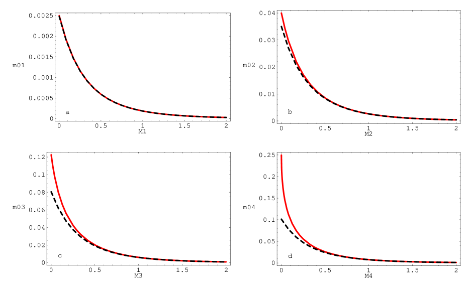
Figure 1: The “lightest” state mass $m_{0}$ as a function of $MR$ for different values of $\omega$: a) 0.05; b) 0.2; c) 0.35 and d) 0.5. Full line (red) is the numerical result from (3.7) and dashed-line (black) the analytical approximation in (3.8).

The wave function corresponding to the eigenvalue (3.8) is given, for $M>0$, by

$$\varphi_{1}^{0}= \sqrt{2|M|R}\ \cos\left[\omega\left(\frac{y}{R}-\pi\right)\right]e^{M(y-\pi R)}\quad;$$

$$\varphi_{2}^{0}= \sqrt{2|M|R}\ \sin\left[\omega\left(\frac{y}{R}-\pi\right)\right]e^{M(y-\pi R)}\quad.$$ (3.9)

and for $M<0$, by

$$\varphi_{1}^{0}= \sqrt{2|M|R}\ \cos\left[\frac{\omega y}{R}\right]e^{-|M|y}\quad;$$

$$\varphi_{2}^{0}= \sqrt{2|M|R}\ \sin\left[\frac{\omega y}{R}\right]e^{-|M|y}\quad.$$ (3.10)

where we have taken the approximation $|M|\pi R>1$ that is well justified from Fig. 1. The even-parity $\varphi^{0}_{1}$ state described by the wave function (3) is quasi-localized at the brane $y=\pi R$, while the one described by (3) is quasi-localized at the brane $y=0$. Notice that these become strictly localized in the limit $\left|M\right|\to\infty$.

The EOM of fermions $\psi$ are easily obtained from the Lagrangian (3.1). Decomposing $\psi$ into 4D chiralities, $\psi_{L,R}$ and assigning an even (odd) parity to $\psi_{L}$ ($\psi_{R}$) one can decompose the fields in plane-waves, $\psi_{L,R}(x,y)=\mathrm{exp}(-ip\cdot x)\,\varphi_{1,2\,}(y)\,\xi$, where $p^{2}=m^{2}$ with $m$ the mass eigenvalues, $\varphi_{1,2\,}(y)$ the mass eigenfunctions, and $\xi$ is a constant two-component spinor. From here on one could perform a similar analysis to the bosonic case, taking into account that fermions are not affected by the SS-breaking, as shown in (3.1). However this is not necessary since we can use supersymmetry to write the final result. In fact the mass eigenvalues are given by (3.7) for $\omega=0$, i.e.

$$m_{n}^{2}=\frac{n^{2}}{R^{2}}+M^{2}\left(1-\delta_{n0}\right)\quad.$$ (3.11)

In particular the lightest eigenstate is massless, $m_{0}=0$. The corresponding eigenfunctions $\varphi_{1,2}^{0}(y)$ can be read off from Eqs. (3) and (3) with $\omega=0$. The even fermions $\psi_{L}^{0}$ are then quasi-localized at the branes $y=0,\pi R$ depending on the sign of the bulk mass $M$.

4 Effective potential

The first step in the dynamical determination of $\omega$ is to compute the contribution of hypermultiplets to the effective potential $V_{eff}$. We have

$$\begin{split}&V_{eff}=\frac{2N_{H}}{2}\sum_{n}\int\!\!\frac{d^{4}p}{(2\pi)^{4}}\,\text{ln}\left(p^{2}+m^{2}_{n}\right)=2N_{H}\int\!\!\frac{d^{4}p}{(2\pi)^{4}}\,W(p)\quad;\\ &W(p)=\frac{1}{2}\sum_{n}\text{ln}(p^{2}+m_{n}^{2})\quad;\end{split}$$ (4.1)

where $p$ is the 4d Euclidean momentum and $N_{H}$ is the number of hypermultiplets with a common odd bulk mass $M$. Although the mass relation (3.7) cannot be solved analytically, following the techniques of Refs. [12, 13], we can perform the infinite sum to find $W(p)$ - or rather its derivative $\partial_{p}W(p)$ - without requiring explicit analytical expressions for the KK masses. First, we convert the sum over KK mass-eigenvalues into a contour integral $C$ around the infinite set of solutions of Eq. (3.7) along the real axis:

$$\frac{\partial\,W}{\partial\,p}= \,p\,\sum_{n}\frac{1}{p^{2}+m_{n}^{2}}=\,p\,\int_{C}\frac{dz}{2\pi i}\,\frac{1}{\left(p^{2}+z^{2}\right)}\,\frac{d}{dz}\text{ln}\,K(z)\quad;$$ (4.2)

$${\rm where}\hskip 22.76219ptK(z)= \left(z^{2}-M^{2}\right)\,\sin^{2}(\omega\pi)-m^{2}\,\sin^{2}\left(\pi R\sqrt{\vrule height=10.0pt,width=0.0ptz^{2}-M^{2}}\right)\quad.$$ (4.3)

The contour $C$ encircles all the eigenvalues on the real axis, but avoids the poles of the integrand in Eq. (4.2) at $z=\pm i\,p$. We can deform $C$ into another contour $C^{\prime}$ around the imaginary axis, with a small circular deformation close to the poles at $z=\pm i\,p$. Since the integrand is odd in $p$ along the imaginary axis, we find that only the residues at $z=\pm ip$ contribute. The final result is

$$W(p,\omega)=\frac{1}{2}\,\text{ln}\left[\left(p^{2}+M^{2}\right)\cos(2\omega\pi)-M^{2}-p^{2}\,\text{cosh}\left(2\pi R\sqrt{p^{2}+M^{2}}\right)\right]+{\rm const}\,.$$ (4.4)

Note that due to 5D supersymmetry and Lorentz invariance, we cannot write a local operator using only $V_{5}^{2}$, which implies that (at one loop) $V_{eff}$ must be finite. Indeed the divergent part is $\omega$-independent, which can be shown by subtracting the fermionic part $W(p,\omega=0)$:

$$V_{eff}= \,2N_{H}\,\int\!\!\frac{d^{4}p}{(2\pi)^{4}}\,\left[\vrule height=14.0pt,width=0.0ptW(p,\omega)-W(p,\omega=0)\right]$$ (4.5)

$$= \,\frac{2N_{H}}{2}\,\int\!\!\frac{d^{4}p}{(2\pi)^{4}}\,\text{ln}\left[1+\frac{\left(p^{2}+M^{2}\right)\,\sin^{2}(\omega\pi)}{p^{2}\,\text{sinh}^{2}\left(\pi R\,\sqrt{p^{2}+M^{2}}\right)}\right]\quad.$$

In the limit of vanishing bulk mass, Eq. (4.5) recovers the standard expression for the effective potential involving polylogarithms in Eq. (1.3).

It is also convenient to find an analytical expression for $V_{eff}$ in Eq. (4.5) in the limit that $2|M|\pi R>1$. We have

$$V_{eff}\simeq\frac{2N_{H}}{2}\,\int\!\!\frac{d^{4}p}{(2\pi)^{4}}\,\text{ln}\left[1+\frac{4\,\left(p^{2}+M^{2}\right)}{p^{2}}\sin^{2}(\omega\pi)\,e^{-2M\,\pi\,R\,\sqrt{1+\frac{p^{2}}{M^{2}}}}\right]\quad;$$ (4.6)

which can be computed analytically by expanding the logarithm to give

$$V_{eff}\simeq\frac{2N_{H}}{32\pi^{6}R^{4}}\sin^{2}(\omega\pi)\ F(M\pi R)\quad;$$ (4.7)

where

$$F(x)=e^{-2x}\left[3+6x+6x^{2}+4x^{3}\right]\quad.$$ (4.8)

We have checked numerically that (4.7) is a good approximation of (4.5) when $2|M|\pi R>1$.

5 Dynamical determination of SS-parameter

The effective potential in (4.7) arising from bulk fields with an odd parity mass has a minimum at $\omega=0$ and a maximum at $\omega=1/2$. However, when this is combined with the potential (1.3) generated by bulk fields without bulk masses for the cases where it has a minimum at $\omega=1/2$ and a maximum at $\omega=0$, the resulting total potential can have a global minimum at intermediate values $0<\omega<1/2$. In fact if we have a situation where the number of hypermultiplets with zero bulk masses $N_{h}$ is such that $N_{h}<2+N_{V}$ and the potential (1.3) has a minimum at $\omega=1/2$, then by adding $N_{H}$ hypermultiplets with a common mass $M$, the critical value of the mass $M^{*}$ for which $\omega=1/2$ becomes a maximum and the minimum is shifted to $\omega<1/2$ is provided by the solution of the following equation,

$$9(2+N_{V}-N_{h})\,\zeta(3)=4N_{H}\ F(M^{*}\pi R)\quad;$$ (5.1)

which is valid for values $|M|\pi R\stackrel{{\scriptstyle>}}{{{}_{\sim}}}1$ for which the approximation leading to (4.7) holds. For instance, consider the case where all three generations of quarks and leptons live in the bulk with a common mass $M>0$. From Eq. (5.1) we find that the minimum at $\omega=1/2$ is destabilized for values of $M^{*}R\simeq 0.78$.

Figure 2: Effective potential (in units of $10^{-4}$) with $N_{V}=12$, $N_{h}=0$ and $N_{H}=45$ for values of $MR=0.72$ (full), $0.74$ (dashed), $0.76$ (dot-dashed) and $0.78$ (dots).

This is shown in Fig. 2 where the effective potential is plotted as a function of $\omega$ for several values of $M$ and in Fig. 3 where the minimum of $\omega$ is plotted as a function of $MR$. Of course if there are several sets of hypermultiplets with different masses (localizations) those with smaller masses (less localized) provide the leading contribution to the effective potential. For instance in the example above, localized states with masses $MR\gg 1$ would not alter the dynamical minimization with respect to $\omega$.

Figure 3: Plot of $\omega$ as a function of $MR$ for the particle content of Fig. 2

6 Conclusions

In this paper we have shown that the SS-mechanism for supersymmetry breaking in five-dimensional orbifold theories is affected by the level of localization of five-dimensional fields on boundaries. Indeed, the SS supersymmetry breaking parameter $\omega$ turns out to be a function of the localizing mass term $M$. The value of the VEV of the parameter $\omega$ is fixed by one-loop corrections and, in the absence of quasi-localized five-dimensional fields, is fixed to be either 0 or 1/2 depending on the number of bulk hypermultiplets and vector multiplets. However, with quasi-localized fields, the VEV of the SS parameter can assume any intermediate value.

Our results can be generalized to the case in which the five-dimensional symmetry is a gauge symmetry. This is particularly interesting in theories where the Standard Model Higgs boson can be identified with the extra dimensional component of a gauge boson and the higher dimensional gauge group is broken to the Standard Model group by the orbifold action. In that case the Standard Model symmetry can be radiatively broken by the Hosotani mechanism and the Higgs boson mass is protected from bulk quadratic divergences by the higher dimensional gauge theory without any need for supersymmetry [14]. We are presently investigating how our results can be extended to such theories in order to reproduce satisfactory Yukawa couplings and Higgs potentials.

Acknowledgements

This work was supported in part by the RTN European Programs HPRN-CT-2000-00148 and HPRN-CT-2000-00152 and by CICYT, Spain, under contracts FPA 2001-1806 and FPA 2002-00748. The work of GG was supported by DAAD. AR thanks IFAE for hospitality during the completion of this work.

References

- [1] Y. Hosotani, Phys. Lett. B 126 (1983) 309; ibidem, Phys. Lett. B 129 (1983) 193; ibidem, Annals Phys. 190 (1989) 233.
- [2] J. Scherk and J. H. Schwarz, Phys. Lett. B 82 (1979) 60; ibidem, Nucl. Phys. B153 (1979) 61.
- [3] A. Pomarol and M. Quiros, Phys. Lett. B 438 (1998) 255 [arXiv:hep-ph/9806263]; I. Antoniadis, S. Dimopoulos, A. Pomarol and M. Quiros, Nucl. Phys. B 544 (1999) 503 [arXiv:hep-ph/9810410]; R. Barbieri, L. J. Hall and Y. Nomura, Phys. Rev. D 63 (2001) 105007 [arXiv:hep-ph/0011311]; N. Arkani-Hamed, L. J. Hall, Y. Nomura, D. R. Smith and N. Weiner, Nucl. Phys. B 605 (2001) 81 [arXiv:hep-ph/0102090]; A. Delgado and M. Quiros, Nucl. Phys. B 607 (2001) 99 [arXiv:hep-ph/0103058]; A. Delgado, G. von Gersdorff, P. John and M. Quiros, Phys. Lett. B 517 (2001) 445 [arXiv:hep-ph/0104112]; R. Contino and L. Pilo, Phys. Lett. B 523 (2001) 347 [arXiv:hep-ph/0104130]; Y. Nomura, arXiv:hep-ph/0105113; N. Weiner, arXiv:hep-ph/0106021; R. Barbieri, L. J. Hall and Y. Nomura, Nucl. Phys. B 624 (2002) 63 [arXiv:hep-th/0107004]; A. Masiero, C. A. Scrucca, M. Serone and L. Silvestrini, Phys. Rev. Lett. 87 (2001) 251601 [arXiv:hep-ph/0107201]; A. Delgado, G. von Gersdorff and M. Quiros, Nucl. Phys. B 613 (2001) 49 [arXiv:hep-ph/0107233]; M. Quiros, J. Phys. G 27 (2001) 2497; V. Di Clemente, S. F. King and D. A. Rayner, Nucl. Phys. B 617 (2001) 71 [arXiv:hep-ph/0107290]; V. Di Clemente and Y. A. Kubyshin, Nucl. Phys. B 636 (2002) 115 [arXiv:hep-th/0108117]; D. M. Ghilencea, H. P. Nilles and S. Stieberger, New J. Phys. 4 (2002) 15 [arXiv:hep-th/0108183]; H. D. Kim, Phys. Rev. D 65 (2002) 105021 [arXiv:hep-th/0109101]; T. Gherghetta and A. Riotto, Nucl. Phys. B 623 (2002) 97 [arXiv:hep-th/0110022]; V. Di Clemente, S. F. King and D. A. Rayner, Nucl. Phys. B 646 (2002) 24 [arXiv:hep-ph/0205010].
- [4] G. von Gersdorff and M. Quiros, Phys. Rev. D 65 (2002) 064016 [arXiv:hep-th/0110132].
- [5] For a review, see: M. Quiros, “New ideas in symmetry breaking,” Lectures given at TASI 2002, Boulder, Colorado, 2-28 Jun 2002, arXiv:hep-ph/0302189.
- [6] G. von Gersdorff and M. Quiros, arXiv:hep-th/0305024.
- [7] G. von Gersdorff, M. Quiros and A. Riotto, Nucl. Phys. B 634 (2002) 90 [arXiv:hep-th/0204041].
- [8] H. Georgi, A. K. Grant and G. Hailu, Phys. Rev. D 63 (2001) 064027 [arXiv:hep-ph/0007350]; N. Arkani-Hamed, A. G. Cohen and H. Georgi, Phys. Lett. B 516 (2001) 395 [arXiv:hep-th/0103135].
- [9] D. M. Ghilencea, S. Groot Nibbelink and H. P. Nilles, Nucl. Phys. B 619 (2001) 385 [arXiv:hep-th/0108184].
- [10] R. Barbieri, R. Contino, R. Creminelli, R. Rattazzi and C. A. Scrucca Phys. Rev. D. 66 (2002) 024025 [arXiv:hep-th/0203039]; D. Marti and A. Pomarol, Phys. Rev. D 66 (2002) 125005 [arXiv:hep-ph/0205034].
- [11] G. von Gersdorff, L. Pilo, M. Quirós, D. A. Rayner and A. Riotto, in preparation.
- [12] A. Delgado, A. Pomarol and M. Quiros, Phys. Rev. D 60 (1999) 095008 [arXiv:hep-ph/9812489].
- [13] W. D. Goldberger and I. Z. Rothstein, hep-th/0208060.
- [14] I. Antoniadis, K. Benakli and M. Quiros, New J. Phys. 3 (2001) 20 [arXiv:hep-th/0108005]; G. von Gersdorff, N. Irges and M. Quiros, Nucl. Phys. B 635 (2002) 127 [arXiv:hep-th/0204223]; G. von Gersdorff, N. Irges and M. Quiros, arXiv:hep-ph/0206029; C. Csaki, C. Grojean and H. Murayama, Phys. Rev. D 67 (2003) 085012 [arXiv:hep-ph/0210133]; G. von Gersdorff, N. Irges and M. Quiros, Phys. Lett. B 551 (2003) 351 [arXiv:hep-ph/0210134]; G. Burdman and Y. Nomura, Nucl. Phys. B 656 (2003) 3 [arXiv:hep-ph/0210257]; C. A. Scrucca, M. Serone and L. Silvestrini, arXiv:hep-ph/0304220.