TPJU-03/2003
  
An attempt to construct pion distribution amplitude
from the PCAC relation
in the nonlocal chiral quark model
 

Abstract

Using the PCAC relation, we derive a compact formula for the pion decay constant $F_{\pi}$ in the nonlocal chiral quark model. For practical calculations this formula may be used both in the Minkowski and in the Euclidean space. For the pion momentum $P_{\mu}\rightarrow 0$ it reduces to the well known expression derived earlier by other authors. Using a generalized dipole Ansatz for the momentum dependence of the constituent quark mass in the Minkowski space, we express $F_{\pi}^{2}$ in terms of a single integral over the quark momentum fraction $u$. We interpret the integrand as a pion distribution amplitude $\phi(u)$. We discuss its properties and compare with the $\pi$DA’s obtained in other models.

1 Introduction

Recent data from CLEO [1] and E791[2] experiments triggered a new wave of theoretical studies of the leading twist pion distribution amplitude ($\pi$DA). On one side the data have been reanalyzed taking into account NLO perturbative QCD effects, as well as nonperturbative effects parameterized within the QCD light-cone sum rules [3],[4]. On the other hand nonperturbative models [5]–[13] and lattice QCD [14]–[17] have been employed to calculate the $\pi$DA from the relatively nonrestrictive physical assumptions. Here the dual nature of the pion, being the quark–antiquark bound state and the Goldstone boson of the broken chiral symmetry at the same time, makes such calculations interesting by itself, even if the data is not yet decisive enough to distinguish between different models.

Pion distribution amplitude is usually defined by means of the following matrix element (see e.g. [18]):

$$\phi_{\pi}(u) =\frac{1}{i\sqrt{2}F_{\pi}}\int\limits_{-\infty}^{\infty}\frac{d\tau}{\pi}e^{-i\tau(2u-1)(nP)}$$

$$\left\langle 0\left|\bar{d}(n\tau)\hbox to0.0pt{/\hss}n\gamma_{5}u\left(-n\tau\right)\right|\pi^{+}(P)\right\rangle$$ (1)

in the light cone kinematics where two quarks separated by the light cone distance $z=2\tau$ along the direction $n=(1,0,0,-1)$ are moving along the light cone direction $\tilde{n}=(1,0,0,1)$ parallel to the total momentum $P$. Here $F_{\pi}=93$ MeV. In this kinematical frame any four vector $v$ can be decomposed as:

$$v^{\mu}=\frac{v^{+}}{2}\tilde{n}^{\mu}+\frac{v^{-}}{2}n^{\mu}+v_{\bot}^{\mu}$$ (2)

with $v^{+}=n\cdot v,\quad v^{-}=\tilde{n}\cdot v$, and the scalar product of two four vectors reads:

$$v\cdot w=\frac{1}{2}v^{+}w^{-}+\frac{1}{2}v^{-}w^{+}-\vec{v}_{\bot}\cdot\vec{w}_{\bot}.$$ (3)

In Eq.(1) the path ordered exponential of the gluon field, required by the gauge invariance, has been omitted since we shall be working in the effective quark model where the gluon fields have been integrated out.

In the local limit matrix element (1) reduces to

$$\left\langle 0\left|A_{\mu}^{a}(x)\right|\pi^{b}(P)\right\rangle=-iP_{\mu}F_{\pi}\delta^{ab}e^{-iPx}$$ (4)

where

$$A_{\mu}^{a}(x)=\bar{\psi}(x)\gamma_{\mu}\gamma^{5}\frac{\tau^{a}}{2}\psi(x)$$ (5)

is the properly normalized axial vector current.

In Refs.[13] $\phi_{\pi}(u)$ has been calculated in the effective chiral quark model in which quarks interact nonlocally with an external meson field

$$U^{\gamma_{5}}(x)=e^{i\gamma_{5}\tau^{a}\pi^{a}(x)/F_{\pi}}$$ (6)

and acquire a momentum dependent constituent mass

$$M(k)=M_{k}=MF(k)^{2}.$$ (7)

$M$ is a constituent quark mass of the order of $350$ MeV and $F(k)$ is a momentum dependent function such that $F(0)=1$ and $F(k^{2}\rightarrow\infty)\rightarrow 0$. Function $F(k)$ embodies nonperturbative effects due to the nontrivial structure of the QCD vacuum. Indeed, $F(k)$ has been explicitly derived within the instanton model [19]. In Refs.[13] where the calculations were performed in the Minkowski space (instanton model is inevitably formulated in the Euclidean metric) a convenient Ansatz for $F(k)$ was used:

$$F(k)=\left(\frac{-\Lambda^{2}}{k^{2}-\Lambda^{2}+i\epsilon}\right)^{n}.$$ (8)

With this Ansatz $\phi_{\pi}(u)$ as well as higher twist $\pi$DA’s were calculated in Refs.[13] and [20] respectively.

The problem is, however, that in the model with the nonlocal interaction (and momentum dependent quark mass $M_{k}$) the axial current (5) does not exhibit PCAC [21]–[24]. More drastically, a naive vector current

$$V_{\mu}^{a}(x)=\bar{\psi}(x)\gamma_{\mu}\frac{\tau^{a}}{2}\psi(x)$$ (9)

is not conserved. In order to restore these properties extra currents have to be added to $A_{\mu}^{a}$ and $V_{\mu}^{a}$ [22],[23]. These new pieces modify both model expressions for $F_{\pi}$ and for $\phi_{\pi}(u)$. While the formula for $F_{\pi}$ is well known in terms of the Euclidean integral [23],[25]:

$$F_{\pi}^{2}=4N_{c}\int\frac{d^{4}k_{E}}{(2\pi)^{4}}\frac{M_{k}^{2}-k_{E}^{2}M_{k}M_{k}^{\prime}+k_{E}^{4}M_{k}^{\prime 2}}{(k_{E}^{2}+M_{k}^{2})^{2}}$$ (10)

(here $M_{k}^{\prime}=dM_{k}/dk^{2})$ the form of the wave function has been a subject of different studies with, however, contradictory results. For example the distribution amplitude obtained in Ref.[8] is very close to the asymptotic form

$$\phi_{\pi}^{as}(u)=6u(1-u)$$ (11)

where $u=k^{+}/P^{+}$ is the momentum fraction carried by the quark, whereas in Refs.[9]–[11] $\phi_{\pi}(u)=1$.

In the present work we derive the Minkowski space formula for $F_{\pi}^{2}$ for the modified axial current replacing the naive current in Eq.(4). Our formula, when continued to the Euclidean space, reduces to Eq.(10). However, when evaluated in the Minkowski space by methods developed in Refs.[13], it can be represented as an integral over $du$ from an integrand which we interpret as $\phi_{\pi}(u)$. This function does not resemble (11) and is compatible rather with the constant wave function of Refs.[9]–[11] than with the result obtained in the same model [13], however, with the naive current (5).

There are several comments which are due at this point. First of all it is not clear how the modified current can be generalized to the bilocal operator entering formula (1). That is why it was argued in Refs. [8]–[11] that rather than considering matrix elements of the form (1) or (4), one should calculate the whole physical process in the effective model, impose Bjorken limit to make contact with the expressions known from QCD and extract the distribution amplitude. One has to note however, that the effective models are not valid at large momenta which are needed to impose Bjorken limit. Moreover it is not clear whether the distribution amplitudes defined that way are universal. Secondly, arguments may be given that it is not necessary to insist that the bilocals defining the distribution amplitudes must reduce to the proper currents in the local limit. Indeed, as we shall show below the naive bilocal (1) reproduces the Pagels-Stokar formula [26] for $F_{\pi}^{2}$:

$$F_{\pi}^{2}=4N_{c}\int\frac{d^{4}k_{E}}{(2\pi)^{4}}\frac{M_{k}^{2}-\frac{1}{2}k_{E}^{2}M_{k}M_{k}^{\prime}}{(k_{E}^{2}+M_{k}^{2})^{2}}$$ (12)

which was obtained from the Ward-Takahshi identities.

2 Currents in the nonlocal models

Let us consider the model defined by an action [12],[13]:

$$S=\,\int(dk)\bar{\psi}(k)\left(\hbox to0.0pt{/\hss}{k}-m\right)\psi(k)-M\int(dk\,dl)\bar{\psi}(l)F(l)U^{\gamma_{5}}(l-k)F(k)\psi(k).$$

Here, following [24] $(dk)=d^{4}k/(2\pi)^{4}$ etc., and $(dx)=d^{4}x$. Equations of motion for the quark fields read

$$\hbox to0.0pt{/\hss}{k}\psi(k) =M\int(dl)F(k)U^{\gamma_{5}}(k-l)F(l)\psi(l)+m\psi(k),$$

$$\bar{\psi}(k)\hbox to0.0pt{/\hss}{k} =M\int(dl)\bar{\psi}(l)F(l)U^{\gamma_{5}}(l-k)F(k)+m\bar{\psi}(k).$$ (13)

To get the equation of motion for the $U^{\gamma_{5}}$ field let us expand (6)

$$U^{\gamma_{5}}(l-k)=(2\pi)^{4}\delta^{(4)}(l-k)+\frac{i}{F_{\pi}}\gamma^{5}\tau^{c}\pi^{c}(l-k)+\ldots$$ (14)

and the equation of motion gives a constraint

$$\int(dl)\,\bar{\psi}(l+k)F(l+k)\gamma^{5}\tau^{a}F(l)\psi(l)=0.$$ (15)

It is easy to verify that the naive vector current (9) is not conserved [23],[24]. In order to restore current conservation, the following two currents have to be added to $V_{\mu}^{a}$ (in momentum space)

$$\tilde{V}_{\mu}^{a}(P)=V_{\mu}^{a}(P)+R_{\mu}^{a}(P)+L_{\mu}^{a}(P)$$ (16)

with left and right currents defined as

$$L_{\mu}^{a}(P) =iM\int(dx\,dy\,dz)\,\int\limits_{x}^{z}ds_{\mu}e^{iPs}\,\bar{\psi}(x)F(x-z)T^{a}U^{\gamma_{5}}(z)F(z-y)\psi(y),$$

$$R_{\mu}^{a}(P) =iM\int(dx\,dy\,dz)\,\int\limits_{z}^{y}ds_{\mu}e^{iPs}\,\bar{\psi}(x)F(x-z)U^{\gamma_{5}}(z)T^{a}F(z-y)\psi(y)$$ (17)

where $T^{a}=\tau^{a}/2$. Accordingly the modified axial current reads:

$$\tilde{A}_{\mu}^{a}(P)=A_{\mu}^{a}(P)+R_{\mu}^{a}(P)-L_{\mu}^{a}(P)$$ (18)

with $T^{a}=\gamma_{5}\tau^{a}/2$. The integral $ds_{\mu}$ should be understood as an integral over the path connecting points $z$ and $y$ or $x$. This prescription makes the $L_{\mu}^{a}$ and $R_{\mu}^{a}$ currents path dependent [23] (strictly speaking the transverse part is not fixed).

The divergence of the modified vector current is, however, path independent and takes the following form:

$$P^{\mu}\tilde{V}_{\mu}^{a}(P)=M\int(dk\,dl)\,\bar{\psi}(k)F(k)\left[\frac{\tau^{a}}{2},U^{\gamma_{5}}(k-l+P)\right]F(l)\psi(l).$$ (19)

This is immediately zero for the baryon current ($\tau^{a}=1$). For the isospin current we can expand $U^{\gamma_{5}}$ (14)

$$\left[\frac{\tau^{a}}{2},U^{\gamma_{5}}(k-l+P)\right]=\frac{1}{F_{\pi}}\gamma^{5}\tau^{a}\epsilon^{abc}\pi^{c}(k-l+P)+\ldots$$ (20)

and (19) vanishes due to the constraint (15). For the axial current we get

$$P^{\mu}\tilde{A}_{\mu}^{a}(P) =-m\int(dk)\bar{\psi}(k)\gamma_{5}\tau^{a}\psi(k+P)$$

$$-M\int(dk\,dl)\bar{\psi}(k)F(k)\left\{\gamma_{5}\frac{\tau^{a}}{2},U^{\gamma_{5}}(k-l+P)\right\}_{+}F(l)\psi(l).$$ (21)

By expanding $U^{\gamma_{5}}$ (14) we arrive at

$$P^{\mu}\tilde{A}_{\mu}^{a}(P) =-m\int(dk)\bar{\psi}(k)\gamma_{5}\tau^{a}\psi(k+P)$$

$$-M\int(dk)\bar{\psi}(k)F(k)\gamma_{5}\tau^{a}F(k+P)\psi(k+P)$$

$$-i\frac{M}{F_{\pi}}\int(dk\,dl)\bar{\psi}(k)F(k)F(l)\psi(l)\,\pi^{a}(k-l+P)+\ldots$$ (22)

which is the proper PCAC formula (note that the second term vanishes due to (15)).

In order to calculate $F_{\pi}$ we can either use Eq.(4) with $A_{\mu}^{a}\rightarrow\tilde{A}_{\mu}^{a}$ [27] or use the PCAC relation

$$\left\langle 0\left|i\partial^{\mu}\tilde{A}_{\mu}^{a}(x)\right|\pi^{b}(P)\right\rangle=-iP^{2}F_{\pi}\delta^{ab}e^{-iPx}$$ (23)

which is what we are going to do in this work. Notice, that we have to calculate the matrix element in Eq.(23) off-shell, extract the leading power in $P^{2}$ and take the limit $P^{2}\rightarrow 0$.

3 Decay constant and the distribution amplitude

3.1 Matrix elements

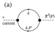
Figure 1: Diagrams contributing to the matrix element of Eq. (21). Black squares denote $\tau^{a,b}\gamma_{5}$.

There are three contributions to the matrix element of Eq.(21) depicted in Fig.1: one from the first term of expansion (14) and two (which by the anticommutation rule reduce to one term, see Eq.(22)) from the term in (14) involving one pion field. Adding all of them we get

$$\left\langle 0\left|i\partial^{\mu}\tilde{A}_{\mu}^{a}(z)\right|\pi^{b}(P)\right\rangle =-\frac{8N_{c}}{F_{\pi}}\delta^{ab}e^{-iPz}\times$$ (24)

$$\int(dk)\left[M_{k}M_{k-P}\frac{k(P-k)+M_{k}M_{k-P}}{(k^{2}-M_{k}^{2})((k-P)^{2}-M_{k-P}^{2})}+\frac{M_{k}^{2}}{k^{2}-M_{k}^{2}}\right].$$

Symmetrizing the last term with respect to the change of variables $k\rightarrow k-P$, adding all terms and comparing with Eq.(23) we arrive at

$$F_{\pi}^{2}=-i4N_{c}\frac{1}{P^{2}}\int(dk)\frac{\left[M_{k}(k-P)_{\mu}-M_{k-P}k_{\mu}\right]^{2}}{(k^{2}-M_{k}^{2})((k-P)^{2}-M_{k-P}^{2})}.$$ (25)

By expanding Eq.(25) in powers of $P^{2}$ we recover the Minkowski version of Eq.(10). Indeed, by changing the variables: $k\rightarrow k+P/2$ we get

$$F_{\pi}^{2}=-i4N_{c}\frac{1}{P^{2}}\int(dk)\frac{1}{2}\frac{\left[M_{k+P/2}(k-\frac{P}{2})_{\mu}-M_{k-P/2}(k+\frac{P}{2})_{\mu}\right]^{2}}{((k+\frac{P}{2})^{2}-M_{k+P/2}^{2})((k-\frac{P}{2})^{2}-M_{k-P/2}^{2})}.$$ (26)

In fact an expression identical to Eq.(26) appears in the axial and pseudoscalar corellators derived within the instanton model of the QCD vacuum [25].

Noting that

$$M_{k\pm P/2}=M_{k}\pm(kP)M_{k}^{\prime}+\frac{P^{2}}{4}M_{k}^{\prime}+\ldots$$ (27)

where ^′ denotes $d/dk^{2}$ we have

$$F_{\pi}^{2}=-i4N_{c}\frac{1}{P^{2}}\int(dk)\frac{P^{2}M_{k}^{2}-4(Pk)^{2}M_{k}M_{k}^{\prime}+4k^{2}(kP)^{2}M_{k}^{\prime 2}}{((k+\frac{P}{2})^{2}-M_{k+P/2}^{2})((k-\frac{P}{2})^{2}-M_{k-P/2}^{2})}.$$ (28)

Since under the integral $k_{\mu}k_{\nu}\rightarrow\frac{1}{4}g_{\mu\nu}k^{2}$ (plus a term proportional to $P_{\mu}P_{\nu}$ which we may safely neglect) equation (28) transforms into

$$F_{\pi}^{2} =-i4N_{c}\int(dk)\frac{M_{k}^{2}-k^{2}M_{k}M_{k}^{\prime}+k^{4}M_{k}^{\prime 2}}{((k+\frac{P}{2})^{2}-M_{k+P/2}^{2})((k-\frac{P}{2})^{2}-M_{k-P/2}^{2})}$$

$$=-i4N_{c}\int(dk)\frac{M_{k}^{2}-k^{2}M_{k}M_{k}^{\prime}+k^{4}M_{k}^{\prime 2}}{(k^{2}-M_{k}^{2})^{2}}.$$ (29)

On the other hand, matrix element of the naive current (5), gives [13]

$$F_{\pi}^{2}P_{\mu}=-i4N_{c}\int(dk)\sqrt{M_{k}M_{k-P}}\frac{M_{k-P}k_{\mu}+M_{k}(P_{\mu}-k_{\mu})}{\left(k^{2}-M_{k}^{2}\right)\left((k-P)^{2}-M_{k-P}^{2}\right)}$$ (30)

which by the same steps which led from Eq.(25) to (29) reduces equation (30) to the Minkowski version of the Pagels-Stokar formula (12).

3.2 Calculation of the loop integral

In order to calculate the loop integral in Eq.(25) with $M_{k}$ given by Eqs.(7,8) we shall introduce the light-cone parameterization of the momenta (2) with

$$d^{4}k=\frac{P^{+}}{2}du\,dk^{-}d^{2}\vec{k}_{\bot}$$ (31)

where $k^{+}=uP^{+}$. The method of evaluating $dk^{-}$ integral, taking the full care of the momentum mass dependence, has been given in [13]. To evaluate $dk^{-}$ integral we have to find the poles in the complex $k^{-}$ plane. It is important to note that the poles come only from the momentum dependence in the denominators of Eqs.(25,30). This means that the position of the poles is given by the zeros of denominator, that is by the solutions of the equation

$$k^{2}-M^{2}\left(\frac{\Lambda^{2}}{k^{2}-\Lambda^{2}+i\epsilon}\right)^{4n}+i\epsilon=0.$$ (32)

This equation is equivalent to

$$G(z)=z^{4n+1}+z^{4n}-r^{2}=\prod_{i=1}^{4n+1}(z-z_{i}),$$ (33)

with $z=k^{2}/\Lambda^{2}-1+i\epsilon$ and $r^{2}=M^{2}/\Lambda^{2}$. For $r^{2}\neq 0$ (or finite $\Lambda$) equation (33) has $4n+1$ nondegenerate solutions which we denote $z_{i}$. Equation (32) should be understood as an equation for $k_{i}^{-}=k^{-}(z_{i})$. In general case $4n$ of $z_{i}$’s can be complex and the care must be taken about the integration contour in the complex $k^{-}$ plane. Because of the imaginary part of the $z_{i}$’s, the poles in the complex $k^{-}$ plane can drift across Re$k^{-}$ axis. In this case the contour has to be modified in such a way that the poles are not allowed to cross it. This follows from the analyticity of the integrals in the $\Lambda$ parameter and ensures the vanishing of $\pi$DA’s in the kinematically forbidden regions. The results are expressed as sums over $z_{i}$’s which have to be found numerically.

In order to avoid spurious divergences coming from $k^{-}$ in the numerator of Eq.(29) we shall make use of the Lorentz invariance, writing

$$F_{\pi}^{2}=-i4N_{c}\frac{1}{P^{2}}I_{\mu\nu}g^{\mu\nu}.$$ (34)

Since $I_{\mu\nu}$ vanishes for $P_{\mu}\rightarrow 0$ (see (25) and (29)) we have that

$$I_{\mu\nu}=A(P^{2})P_{\mu}P_{\nu}+\frac{1}{4}B(P^{2})P^{2}g_{\mu\nu}$$ (35)

with

$$A(P^{2})\rightarrow A,\quad B(P^{2})\rightarrow B\quad\text{for}\quad P^{2}\rightarrow 0.$$ (36)

Then

$$F_{\pi}^{2}=-i4N_{c}(A+B)$$ (37)

Hence we have to calculate 2 integrals:

$$A=\frac{1}{P^{+\,2}}n^{\mu}n^{\mu}I_{\mu\nu},\;B=-\frac{4}{P^{2}}\varepsilon_{\bot}^{\mu}\varepsilon_{\bot}^{\nu}I_{\mu\nu}.$$ (38)

The result reads

$$A =-\frac{i}{16\pi^{2}}M^{2}\int\limits_{0}^{1}du\sum_{i,k=1}^{4n+1}f_{i}f_{k}(z_{k}^{2n}\bar{u}+z_{i}^{2n}u)^{2}\times\ln\left(1+z_{i}\bar{u}+z_{k}u\right),$$ (39)

$$B =-\frac{i}{16\pi^{2}}\frac{2M^{2}\Lambda^{2}}{P^{2}}\int\limits_{0}^{1}du\sum_{i,k=1}^{4n+1}f_{i}f_{k}(z_{k}^{2n}-z_{i}^{2n})^{2}\left((1+z_{i}\bar{u}+z_{k}u)-\frac{P^{2}}{\Lambda^{2}}u\bar{u}\right)$$

$$\hskip 170.71652pt\times\ln\left((1+z_{i}\bar{u}+z_{k}u)-\frac{P^{2}}{\Lambda^{2}}u\bar{u}\right).$$

Here $\bar{u}=1-u$ and

$$f_{i}=\prod\limits_{\begin{subarray}{c}k=1\\ k\neq i\end{subarray}}^{4n+1}\frac{1}{z_{i}-z_{k}}=\prod\limits_{\begin{subarray}{c}k=1\\ k\neq i\end{subarray}}^{4n+1}\frac{1}{z_{k}-z_{i}}$$ (40)

for which the following identities hold [13]

$$\sum\limits_{i=1}^{4n+1}f_{i}z_{i}^{m}=\left\{\begin{array}[]{ccc}0&&m<4n\\ &&\\ 1&&m=4n\end{array}\right..$$ (41)

As seen from Eq.(39) the first term in $B$ is singular as $P^{2}\rightarrow 0$ in apparent contradiction with the finiteness of $F_{\pi}^{2}$. However, the function

$$\phi_{\inf}(u)=-\frac{N_{c}M^{2}}{2\pi^{2}}\sum_{i,k=1}^{4n+1}f_{i}f_{k}(z_{k}^{2n}-z_{i}^{2n})^{2}(1+z_{i}\bar{u}+z_{k}u)\ln(1+z_{i}\bar{u}+z_{k}u)$$ (42)

vanishes when integrated over $du$. Hence the finite formula for $F_{\pi}^{2}$ reads

$$F_{\pi}^{2}=-\frac{N_{c}M^{2}}{4\pi^{2}}\int\limits_{0}^{1}du\sum_{i,k=1}^{4n+1}f_{i}f_{k}\left[(z_{k}^{2n}\bar{u}+z_{i}^{2n}u)^{2}-2(z_{k}^{2n}-z_{i}^{2n})^{2}u\bar{u}\right]\ln\left(1+z_{i}\bar{u}+z_{k}u\right).$$ (43)

This allows us to define the distribution amplitude

$$\tilde{\phi}_{\pi}(u)=-\frac{N_{c}M^{2}}{4\pi^{2}F_{\pi}^{2}}\sum_{i,k=1}^{4n+1}f_{i}f_{k}\left[(z_{k}^{2n}\bar{u}+z_{i}^{2n}u)^{2}-2(z_{k}^{2n}-z_{i}^{2n})^{2}u\bar{u}\right]\ln\left(1+z_{i}\bar{u}+z_{k}u\right).$$ (44)

Let us recall that the distribution amplitude defined by means of the naive axial current (5) reads [13]

$$\phi_{\pi}(u)=-\frac{N_{c}M^{2}}{4\pi^{2}F_{\pi}^{2}}\sum\limits_{i,k}f_{i}f_{k}\,(z_{i}^{n}z_{k}^{3n}\bar{u}+z_{i}^{3n}z_{k}^{n}u)\ln\left(1+z_{i}\bar{u}+z_{k}u\right).$$ (45)

3.3 Numerical results

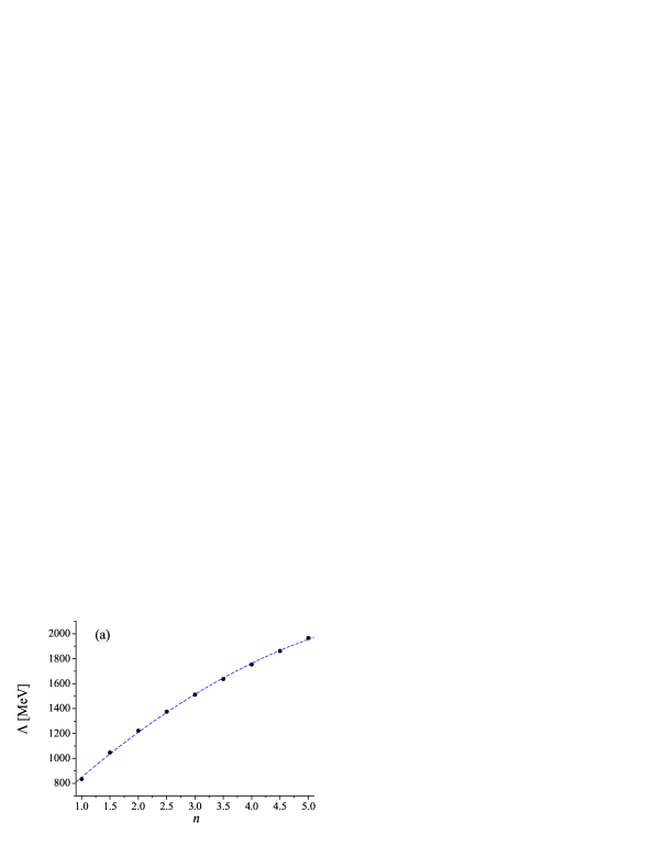
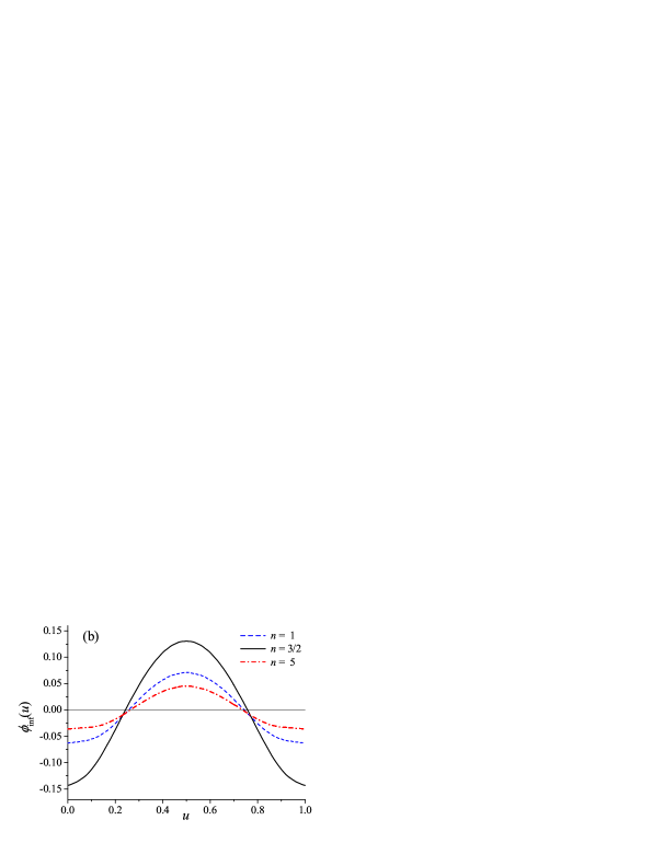
Figure 2:  a) dots: cutoff parameter $\Lambda$ for different $n$ (Eq.(8)) and for $M=350$ MeV, dahed line: fit described in the text; b) function $\phi_{\inf}(u)$ for $n=3/2,$ $3$ and $5$.

Condition (10), or equivalently (43) provide a relation between parameter $\Lambda$, constituent mass $M$ and power $n$ from Eq.(8). Throughout this paper we shall use $M=350$ MeV. The value of parameter $\Lambda=\Lambda(n)$ obtained from Eq.(43), or from Eq.(10) after continuation of the cutoff formula (8) to the Euclidean metric, is depicted in Fig.2.a. It is interesting to note, that our formula (43) for $F_{\pi}^{2}$, unlike equation (30), does allow for half integer $n$’s. An approximate relation, depicted by a dashed line in Fig.2.a holds

$$\Lambda[\text{MeV}]=432.82+444.61\,n-28.02\,n^{2}.$$

The local current (5) contributes, through Eq.(12), approximately 70% to the total normalization.

Having fixed $\Lambda$ for given $n$, we can calculate the distribution amplitude as defined by Eq.(44). However, before doing this we have to check whether the formally divergent part, given as an integral over $u$ from the function $\phi_{\inf}(u),$ vanishes. We have checked numerically that this is indeed the case. Function $\phi_{\inf}(u)$ is plotted in Fig.2.b for $n=3/2,$ $3$ and $5$.

Next, in Fig.3 we plot the distribution amplitude $\tilde{\phi}_{\pi}(u)$ for $n=3/2$ and $n=5$ (solid lines) together with the contributions from integrals $A$ and $B$ (37). We see that the contribution from $A$ is relatively flat and does not vanish at the end points. The contribution from $B$ vanishes at the end points and is even negative in their vicinity. There is not much difference between the two cases $n=3/2$ and $n=5$, although one may say that the smaller $n$ the flatter $\tilde{\phi}_{\pi}$.

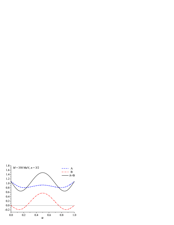
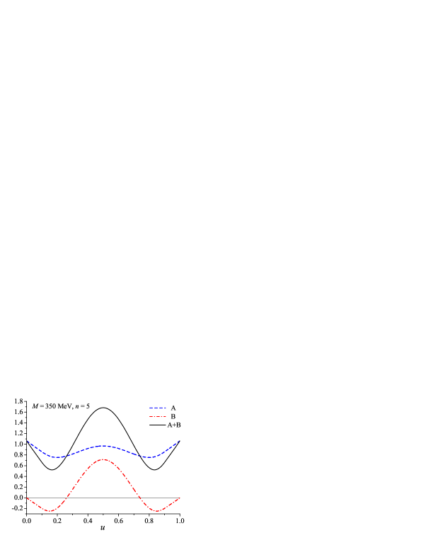
Figure 3:  Function $\tilde{\phi}_{\pi}$ for $n=3/2$ and $n=5$ with two contributions $A$ and $B$ given by Eqs.(39).

In Fig.4.a we plot for comparison function $\tilde{\phi}_{\pi}(u)$ (44), $\phi_{\pi}(u)$ (45) corresponding to the naive axial current (5) for $M=350$ MeV and $n=3$, together with the asymptotic distribution amplitude (11). One should note that while model distributions are defined as some low normalization scale $Q^{2}=\mu^{2}$, $\phi_{\pi}^{as}(u)$ corresponds to the limit $Q^{2}\rightarrow\infty$. Indeed, the leading twist distribution amplitude can be expanded in terms of the Gegenbauer polynomials

$$\phi_{\pi}(u;Q^{2})=6u(1-u)\left[1+\sum\limits_{n=2,4\ldots}^{\infty}a_{n}(Q^{2})C_{n}^{3/2}(2u-1)\right]$$ (46)

where $a_{n}(Q^{2})\rightarrow 0$ in the large $Q^{2}$ limit [28]. It is important no notice that $a_{n}(Q^{2})$ tend to zero monotonically, so that they cannot change the sign.

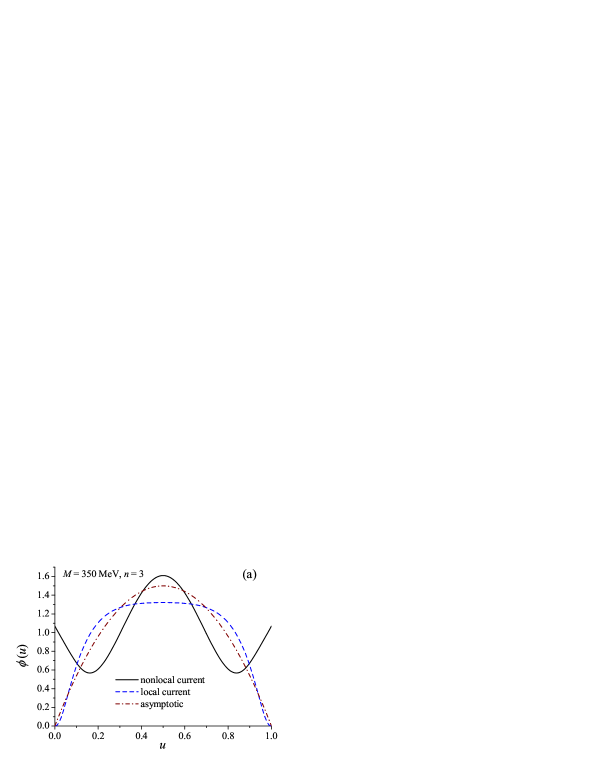
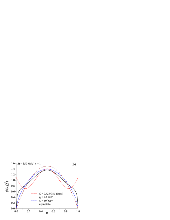
Figure 4:  a): Functions $\tilde{\phi}_{\pi}$ (Eq.(44), solid), $\phi_{\pi}$ (Eq.(45), dashed) for $n=3$ and asymptotic distribution amplitude (Eq.(11), dash-dotted); b): Evolustion of $\tilde{\phi}_{\pi}$ from the initial scale $Q=425$ MeV (dotted line) to the CLEO point $Q=2.4$ GeV (solid) and for $Q=10^{12}$ GeV (dashed) for $n=1$.

As soon as we switch on the QCD evolution, distribution amplitude $\tilde{\phi}_{\pi}(u,Q^{2})$ changes the shape and it goes to zero at the end points. This evolution is plotted in Fig.4.b for $n=1$, assuming 2 light flavors, $\Lambda_{QCD}=175$ MeV, and initial scale $\mu=425$ MeV. This initial scale has been adjusted in such a way, that the second Gegenbauer coefficient $a_{2}$, when evolved to the CLEO point $Q=2.4$ GeV, gives $a_{2}(2.4)=0.15$ as indicated by the analysis of Ref.[3]. For the normalization scale as large as $10^{12}$GeV the evolved distribution is slowly approaching the asymptotic one.

4 Summary and discussion

In the present paper we have derived a compact formula (25) for the pion decay constant in the nonlocal chiral quark model. In order to define $F_{\pi}$ we have used the full nonlocal axial current (18) and the PCAC relation (23). Equation (25), when expanded in the pion momentum $P_{\mu}$, reduces to the well known [23],[25] formula (29). The advantage of Eq.(25) consists in the fact that it can be evaluated in the Minkowski space with a suitable Ansatz for the momentum dependence of the constituent mass (8). By integrating (25) over $dk^{-}$ and $d^{2}\vec{k}_{\bot}$ we are left with a $du$ integral over the function $\tilde{\phi}_{\pi}(u)$ which we interpret as a pion distribution amplitude (44).

As mentioned at the end of Sect.1 it is not clear how to extend the local current (18) to the bilocal operator like the one entering formula (1). Therefore our definition of the pion distribution amplitude may be not correct. However, it is worth to note that the shape of our distribution amplitude resembles a constant DA obtained by a consistent use of the Ward-Takahashi identities [9]–[11], rather than the DA calculated in the instanton model of the QCD vacuum in Ref.[8], although in both approaches full nonlocal currents have been used.

Unfortunately, the $\pi$DA derived here and in Refs.[9]–[11] is probably phenomenologically unacceptable. That is because the detailed analysis of the CLEO data indicates that the coefficient $a_{4}(2.4$ GeV$)$ is negative [3],[4] and possibly as large as $a_{2}(2.4$ GeV$)$ [4]. In our case, however, $a_{4}$ is always positive. The same concerns the constant $\pi$DA. In this respect $\pi$DA derived in by the same methods in Refs.[13] using the bilocal operator (1) with no extra pieces corresponding to the nonlocal currents (17) fits the data much better. That is because, similarly to the results of Refs.[5], it exhibits a shallow minimum around $u=1/2$ which generates negative $a_{4}.$

As already mentioned above, there is a problem how to define the distribution amplitudes in the effective models of QCD. This is due to the fact that the QCD currents and the model currents are not the same. One way would be to perform factorization and large $Q^{2}$ expansion in QCD and then parameterize the nonperturbative matrix elements by a set of unknown distribution amplitudes. To calculate these matrix elements an effective model, like the one discussed here, is used. Considering operators as obtained from QCD leads to the violation of PCAC and, in the worse case, to the violation of the gauge invariance at the level of the effective model. Another method consists in performing factorization and large $Q^{2}$ expansion directly in the effective model. This is possible, since the degrees of freedom of the effective models discussed here are, at least as the quantum numbers are concerned, identical to the degrees of freedom of QCD (except for gluons, which are not present in the former case). This means, however, that the low energy model has to be applied to the processes with large momenum transfer. Since the currents of the effetive models are not the same as in QCD, extra pieces contributing to the DA’s, as compared to the previous method, are present. Although in this work we have not calculated the physical process and have not implemented the Bjorken limit, our approach is in our opinion equivalent, since we have considered the matrix element (4) of the full current (18). Our results indicate that these two methods lead to completely different DA’s . The first method gives the $\pi$DA resembling the asymptotic distribution, whereas the second approach generates the DA which is compatible with a constant.

Acknowledgments

It is a pleasure to dedicate this work to Jan Kwieciński.

We would like to thank A. Rostworowski for comments and for reading the notes. M.P. would like to thank W. Broniowski and E. Ruiz-Arriola for comments and discussion. Special thanks are due to K. Goeke and all members of Inst. of Theor. Phys. II at Ruhr-University where part of this work was completed. M.P. acknowledges support of the Polish State Committee for Scientific Research under grant 2 P03B 043 24.

References

- [1] J. Gronberg (CLEO Collaboration), Phys. Rev. D57 (1998) 33 [hep-ex/9707031].
- [2] E.M. Aitala et al. (Fermilab E791 Collaboration), Phys. Rev. Lett. 86 (2001) 4768 [hep-ex/0010043]; D. Ashery, talk at Workshop on Physics with Electron Polarized Ion Collider, hep-ex/99100024.
- [3] A. Schmedding and O. Yakovlev, Phys. Rev. D62 (2000) 116002 [hep-ph/9905392].
- [4] A.P. Bakulev, S.V. Mikhailov and N.G. Stefanis, Phys. Rev. D67 (2003) 074012 [hep-ph/0212250]; hep-ph/0303039.
- [5] A.P. Bakulev, S.V. Mikhailov and N.G. Stefanis, Phys. Lett. B508 (2001) 279 [hep-ph/0103119]; in: Proceedings of the 36th Rencontres de Moriond, QCD and Hadronic Interactions, hep-ph/0104290.
- [6] T. Heinzl, Ligh-Cone Quantization: Foundations and Applications, Lect. Notes Phys. 572 (2001) 55 [hep-th/0008096]; Nucl. Phys. Proc. Suppl. 90 (2000) 83 [hep-ph/0008314].
- [7] T. Shigetani, K. Suzuki, H. Toki, Phys. Lett. B308 (1993) 383 [hep-ph/9402286]; Nucl. Phys. A579 (1994) 413 [hep-ph/9402277].
- [8] A.E. Dorokhov and L. Tomio, Phys.Rev. D62 (2000) 014016; I.V. Anikin, A.E. Dorokhov and L.Tomio, Phys. Lett. B475 (2000) 361; Phys. Part. Nucl. 31 (2000) 509, (Fiz. Elem. Chast. Atom.Yadra 31 (2000) 1023), A.E. Dorokhov, talk at 37th Rencontres de Moriond, QCD and High Energy Hadronic Interactions, hep-ph/0206088.
- [9] R.M. Davidson and E. Ruiz Arriola, Acta Phys. Polon. B33 (2002) 1791 [hep-ph/0110291]; Phys.Lett. B348 (1995) 163.
- [10] E. Ruiz Arriola, Acta Phys. Polon. B33 (2002) 4443 [hep-ph/0210007].
- [11] E. Ruiz Arriola and W. Broniowski, Phys.Rev. D66 (2002) 094016 [hep-ph/0207266]; Phys.Rev. D67 (2003) 074021 [hep-ph/0301202].
- [12] V.Yu. Petrov and P.V. Pobylitsa, hep-ph/9712203; V.Yu. Petrov, M.V. Polyakov, R. Ruskov, Ch. Weiss and K. Goeke, Phys. Rev. D59 (1999) 114018 [hep-ph/9807229].
- [13] M. Praszałowicz and A. Rostworowski, Phys. Rev. D64 (2001) 074003 [hep-ph/0105188]; talks at 8th Adriatic Meeting, Particle Physics in the New Millennium, hep-ph/0202226 and at 37th Rencontres de Moriond, QCD and High Energy Hadronic Interactions, hep-ph/0205177.
- [14] D. Daniel, R. Gupta and D.G. Richards, Phys. Rev. D43 (1991) 3715.
- [15] L. Del Debbio et al., Nucl. Phys. Proc. Suppl. 83 (2000) 235 [hep-lat/9909147].
- [16] M. Burkardt and H. El-Khozondar, Phys. Rev. D60 (1999) 054504 [hep-ph/9805495]; M. Burkardt and S. Seal, Phys. Rev. D65 (2002) 034501 [hep-ph/0102245 ]; hep-ph/0101338.
- [17] S. Dalley, Phys. Rev. D64 (2001) 036006 [hep-ph/0101318];
- [18] P. Ball, JHEP 9901 (1999) 010 [hep-ph/9812375].
- [19] D.I. Diakonov and V.Yu. Petrov, Nucl. Phys. B245 (1984) 259; B272 (1986) 457.
- [20] M. Praszałowicz and A. Rostworowski, Phys.Rev. D66 (2002) 054002 [hep-ph/0111196]; Acta Phys. Polon. B34 (2003) 2699 [hep-ph/0302269].
- [21] B. Holdom, J. Terning and K. Verbeek, Phys. Lett. B232 (1989) 351, B. Holdom, Phys. Rev. D45 (1992) 2534.
- [22] G. Ripka and R. Ball, in: proceedings of Conference on Many-Body Physics, Coimbra 1993, hep-ph/9312260.
- [23] R.D. Bowler and M. Birse, Nucl. Phys. A582 (1995) 655 [hep-ph/9407336]; R.S. Plant and M. Birse, Nucl. Phys. A628 (1998) 607 [hep-ph/9705372].
- [24] W. Broniowski, in: Miniworkshop on Hadrons as Solitons, Bled 1999, hep-ph/9909438.
- [25] D.I. Dyakonov and V.Yu. Petrov, Sov. Phys. JETP 62 (1985) 431 (Zhur. Eksp. Teor. Fiz. 89 (1985) 751).
- [26] H. Pagels and S. Stokar, Phys. Rev. D20 (1979) 2947.
- [27] A. Bzdak, in preparation.
- [28] A.V. Efremov and A.V. Radyushkin, Theor. Mat. Phys. 42 (1980) 97; Phys. Lett. B94 (1980) 245; S. Brodsky and G.P. Lepage, Phys. Lett. B87 (1979) 594; Phys. Rev. D22 (1980) 2157.