Nonperturbative structure of the quark–gluon vertex

Abstract:

The complete tensor structure of the quark–gluon vertex in Landau gauge is determined at two kinematical points (‘asymmetric’ and ‘symmetric’) from lattice QCD in the quenched approximation. The simulations are carried out at $\beta=6.0$, using a mean-field improved Sheikholeslami–Wohlert fermion action, with two quark masses $\sim 60$ and 115 MeV. We find substantial deviations from the abelian form at the asymmetric point. The mass dependence is found to be negligible. At the symmetric point, the form factor related to the chromomagnetic moment is determined and found to contribute significantly to the infrared interaction strength.

1 Introduction

The quark–gluon vertex describes the coupling between quarks and gluons, and is thus one of the fundamental quantities of QCD. In perturbation theory, a complete calculation has been performed to one loop [1], and partial two- and three-loop calculations have been performed for specific gauges and kinematics [2, 3]. Nonperturbatively, however, it remains largely unknown. In [4, 5, 6] the first steps were taken towards a nonperturbative determination, by way of a quenched lattice calculation of the form factor containing the running coupling in two different kinematics in the Landau gauge.

The Dyson–Schwinger equation (DSE) for the quark propagator contains the quark–gluon vertex, and normal practice has been to truncate the hierarchy of DSEs by providing an ansatz for the vertex. However, if a realistic gluon propagator, obtained from the coupled ghost–gluon(–quark) DSEs [7, 8, 9] and consistent with lattice data [10, 11, 12] is used, dynamical chiral symmetry breaking appears to be quite sensitive to the details of the ansätze employed [9]. It therefore appears highly desirable to obtain ‘hard’ information about the full infrared structure, not only the part containing the running coupling.

In this paper we take the first steps towards this aim, by determining all the nonzero form factors at the two kinematic points used in [6], namely $q=0$ and $q=-2p$, where $q$ is the gluon momentum and $p$ is the momentum of the outgoing quark leg. At the same time we also study the quark mass dependence by using two different quark masses for the vertex at $q=0$. Some preliminary results have already been presented in [13].

The quark–gluon vertex is related to the ghost self-energy through the Slavnov–Taylor identity,

$$q^{\mu}\Gamma_{\mu}(p,q)=G(q^{2})\left[(1-B(q,p+q))S^{-1}(p)-S^{-1}(p+q)(1-B(q,p+q))\right]\,,$$ (1)

where $G(q^{2})$ is the ghost renormalisation function and $B(q,k)$ is the ghost–quark scattering kernel. Evidence from lattice simulations [14] and Dyson–Schwinger equation studies [7, 8, 9] indicate that $G(p^{2})$ is strongly infrared enhanced, and this should also show up in the quark–gluon vertex. On the other hand, nontrivial structure in the ghost–quark scattering kernel, which has usually been assumed to be small, may also be realised in the vertex.

The rest of the paper is structured as follows: In section 2 we briefly present our notation and procedure, referring to [6] for the details. In section 3 we present results for the vertex at the asymmetric point and compare to the abelian (quark–photon) vertex, which is completely determined by the Ward–Takahashi identity at this point. In section 4 we present results for the vertex at the symmetric point, including the ‘chromomagnetic’ form factor $\tau_{5}$. Finally, in section 5 we summarise our results and discuss prospects for further work. Some tree-level formulae used in the analysis are given in the Appendix.

2 Notation and procedure

Throughout this article, we will be using the same notation as in [6], and we refer to that article for a detailed discussion of our notation and procedure. We write the one-particle irreducible (proper) vertex (see fig. 1) as $\Lambda^{a}_{\mu}(p,q)\equiv t^{a}\Lambda_{\mu}(p,q)$, where $p$ and $q$ are the outgoing quark and gluon momentum respectively. The incoming quark momentum is denoted $k$.

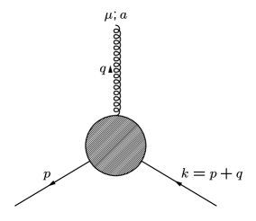
Figure 1: The quark–gluon vertex.

We will be operating in the Landau gauge, where, as discussed in [6], only the transverse-projected part of the vertex can be studied away from $q=0$. We will therefore define the transverse-projected vertex as

$$\Lambda^{P}_{\mu}(p,q)\equiv P_{\mu\nu}(q)\Lambda_{\nu}(p,q)=\Bigl{(}\delta_{\mu\nu}-\frac{q_{\mu}q_{\nu}}{q^{2}}\Bigr{)}\Lambda_{\nu}(p,q)\,.$$ (2)

In a general kinematics the vertex can be decomposed into 12 independent vectors which we can write in terms of vectors $L_{i},T_{i}$ and scalar functions $\lambda_{i},\tau_{i}$ as described in [6]:

$$\Lambda_{\mu}(p,q)=-ig\sum_{i=1}^{4}\lambda_{i}(p^{2},q^{2},k^{2})L_{i,\mu}(p,q)-ig\sum_{i=1}^{8}\tau_{i}(p^{2},q^{2},k^{2})T_{i,\mu}(p,q)\,.$$ (3)

We will here be focusing on the two specific kinematics defined in [6] and related there to the $\widetilde{\text{MOM}}$ and $\overline{\text{MOM}}$ renormalisation schemes — namely, the ‘asymmetric’ point $q=0$ (i.e., $p^{2}=k^{2};q^{2}=0$) and the ‘symmetric’ point $q=-2p$ (i.e., $p^{2}=k^{2}=q^{2}/4$). In the asymmetric kinematics, the vertex reduces to

$$\Lambda_{\mu}(p,0)= -ig\Bigl{[}\lambda_{1}(p^{2},0,p^{2})\gamma_{\mu}-4\lambda_{2}(p^{2},0,p^{2})\not\!pp_{\mu}-2i\lambda_{3}(p^{2},0,p^{2})p_{\mu}\Bigr{]}\,,$$ (4)

while in the symmetric kinematics we have

$$\begin{split}\Lambda_{\mu}(-q/2,q)=&-ig\Bigl{[}\lambda_{1}(q^{2}/4,q^{2},q^{2}/4)\gamma_{\mu}+\tau_{3}(q^{2}/4,q^{2},q^{2}/4)\bigl{(}\not\!qq_{\mu}-q^{2}\gamma_{\mu}\bigr{)}\\ &\phantom{-ig_{0}\Bigl{[}}-i\tau_{5}(q^{2}/4,q^{2},q^{2}/4)\sigma_{\mu\nu}q_{\nu}\Bigr{]}\,;\end{split}$$ (5)

$$\Lambda^{P}_{\mu}(-q/2,q)= -ig\Bigl{[}\lambda^{\prime}_{1}(q^{2}/4,q^{2},q^{2}/4)\bigl{(}\gamma_{\mu}-\not\!qq_{\mu}/q^{2}\bigr{)}-i\tau_{5}(q^{2}/4,q^{2},q^{2}/4)\sigma_{\mu\nu}q_{\nu}\Bigr{]}\,,$$ (6)

where on the last line, in the transverse-projected vertex, we have written $\lambda^{\prime}_{1}\equiv\lambda_{1}-q^{2}\tau_{3}$.

In an abelian theory (QED), the Ward–Takahashi identities imply that the form factors $\lambda_{i}(i=1,2,3)$ are given uniquely in terms of the fermion propagator,

$$S(p)=\frac{1}{i\not\!pA(p^{2})+B(p^{2})}\,=\,\frac{Z(p^{2})}{i\not\!p+M(p^{2})}\,.$$ (7)

In the kinematics we are considering, they are given by

$$\lambda_{1}^{\text{QED}}(p^{2},0,p^{2})=\lambda_{1}^{\text{QED}}(p^{2},4p^{2},p^{2})=A(p^{2})\,;$$ (8)

$$\lambda_{2}^{\text{QED}}(p^{2},0,p^{2})=\frac{1}{2}\frac{\mathrm{d}}{\mathrm{d}p^{2}}A(p^{2})\,;\qquad\lambda_{3}^{\text{QED}}(p^{2},0,p^{2})=-\frac{\mathrm{d}}{\mathrm{d}p^{2}}B(p^{2})\,.$$ (9)

The deviation of the QCD form factors from these expressions thus give us a measure of the purely nonabelian nature of the theory. Note that $\lambda_{4}$, which is identically zero in QED, is zero also in QCD at these two particular kinematic points.

The bare (unrenormalised) quantities $\lambda_{3},\tau_{5}$ and $\lambda^{\prime}_{1}$ (at the symmetric point) can be obtained by tracing the lattice $\Lambda_{\mu}$ with the appropriate Dirac matrix (the identity, $\sigma_{\mu\nu}$ and $\gamma_{\mu}$ respectively):

$$\lambda_{3}(p^{2},0,p^{2}) =\frac{1}{2p^{2}}\sum_{\mu}p_{\mu}\frac{1}{4g_{0}}\operatorname{Re}\operatorname{Tr}\Lambda_{\mu}(p,0)\,;$$ (10)

$$\tau_{5}(q^{2}/4,q^{2},q^{2}/4) =-\frac{1}{3q^{2}}\sum_{\mu,\nu}q_{\mu}\frac{1}{4g_{0}}\operatorname{Re}\operatorname{Tr}\sigma_{\mu\nu}\Lambda^{P}_{\nu}(-q/2,q)\,;$$ (11)

$$\lambda^{\prime}_{1}(q^{2}/4,q^{2},q^{2}/4) =-\frac{1}{3}\sum_{\mu}\frac{1}{4g_{0}}\operatorname{Im}\operatorname{Tr}\gamma_{\mu}\Lambda^{P}_{\mu}(-q/2,q)\,.$$ (12)

At the asymmetric point, $\lambda_{1}$ and $\lambda_{2}$ both come with the same Dirac structure. To separate them, we first determine $\lambda_{1}$ as described in [6] by setting the ‘longitudinal’ momentum component $p_{\mu}$ to zero, and then obtain $\lambda_{2}$ by

$$\lambda_{2}(p^{2},0,p^{2})=\frac{1}{4p^{2}}\sum_{\mu}\Bigl{(}\frac{1}{4g_{0}}\operatorname{Im}\operatorname{Tr}\gamma_{\mu}\Lambda_{\mu}(p,0)+\lambda_{1}(p^{2},0,p^{2})\Bigr{)}\,.$$ (13)

In order to make the lattice form factors more continuum-like, we employ tree-level correction, as discussed in [11, 15]. The tree-level correction of $\lambda_{1}$ is described in [6], although at the symmetric point we have here refined the correction procedure, as described in appendix A. In the case of $\lambda_{2},\lambda_{3}$ and $\tau_{5}$, these are simply zero at tree level in the continuum, while they are non-zero on the lattice with the action and parameters we are using. We therefore have to subtract off the lattice tree-level forms. The details of this are given in appendix A. Not unexpectedly, this procedure leads to large cancellations which make our results unreliable at large momenta.

As always, the quantities obtained from the lattice are bare (unrenormalised) quantities. The relation between renormalised and bare quantities is given by

$$\psi^{0}=Z_{2}^{1/2}\psi\,;\qquad\overline{\psi}^{0}=Z_{2}^{1/2}\overline{\psi}\,;\qquad A_{\mu}^{0}=Z_{3}^{1/2}A_{\mu}\,;\qquad g_{0}=Z_{g}g\,;\qquad\xi_{0}=Z_{3}\xi\,,$$ (14)

where $Z_{2},Z_{3},Z_{g}$ are the quark, gluon and vertex (coupling) renormalisation constants respectively. The renormalised quark and gluon propagator and quark–gluon vertex are related to their bare counterparts according to

$$S^{\text{bare}}(p;a)=Z_{2}(\mu;a)S(p;\mu)\,;\qquad D^{\text{bare}}(q^{2};a)=Z_{3}(\mu;a)D(q^{2};\mu)\,;$$ (15)

$$\Lambda_{\mu}^{\text{bare}}(p,q;a)=Z_{1F}^{-1}(\mu;a)\Lambda_{\mu}(p,q;\mu)\,.$$ (16)

Renormalisation may be carried out in a momentum subtraction scheme. For the quantities computed at the asymmetric point, we will use the $\widetilde{\text{MOM}}$ scheme defined in [6]  requiring that $\lambda_{1}(\mu^{2},0,\mu^{2})=1$; while for the quantities at the symmetric point we will use a modification of the $\overline{\text{MOM}}$ scheme, requiring $\lambda^{\prime}_{1}(\mu^{2}/4,\mu^{2},\mu^{2}/4)=1$. In both cases we choose $\mu=2$ GeV as our renormalisation scale. We can then easily match our results on to perturbation theory in the ultraviolet, using the associated ($\widetilde{\text{MOM}}$ or $\overline{\text{MOM}}$) running coupling.

We use the same ensemble and parameters as in [6]. The Wilson gauge action is used at $\beta=6.0$ on a $16^{3}\times 48$ lattice. The Sommer scale provides an inverse lattice spacing of 2.12 GeV. The mean-field improved SW action is adopted with off-shell improvement in the associated propagators. Further details may be found in [6]. In order to study the quark mass dependence of the vertex, we have used two values for the hopping parameter, $\kappa=0.137$ and 0.1381, corresponding to a bare quark mass $m\approx 115$ and 60 MeV respectively.

3 Asymmetric point

First, we investigate the mass dependence of the $\lambda_{1}$ form factor, which was already studied in [6]. Since in this paper we are primarily concerned with the deviation from the abelian (Ball–Chiu) form, we show, in figure 2, the quantity $Z(p^{2})\lambda_{1}(p^{2},0,p^{2})$, which in an abelian theory would be constant. The clear infrared enhancement observed in [6] is confirmed, and we also see that the mass dependence of this quantity is negligible. The slight difference in $\lambda_{1}$ between the two masses observed in [13] is in other words entirely due to the mass-dependence of the quark renormalisation function.

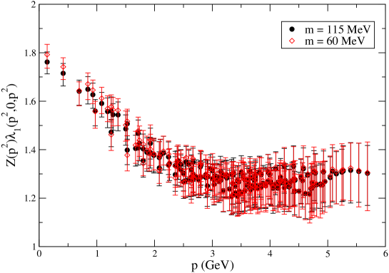
Figure 2: The unrenormalised form factor $\lambda_{1}(p^{2},0,p^{2})$ multiplied by the quark renormalisation function $Z(p^{2})$, as a function of $p$. In an abelian theory, this would be a $p$-independent constant.

In order to compare our results with the abelian forms (9), we have fitted the tree-level corrected quark propagator [15] to the following functional forms [16],

$$Z(p^{2})\equiv 1/A(p^{2}) =k\Biggl{(}1-\frac{c^{2}}{a^{2}p^{2}+l^{2}}\Biggr{)}\,;$$ (17)

$$aM(p^{2})\equiv aB(p^{2})/A(p^{2}) =c_{m}\frac{l_{m}^{2(\alpha-1)}}{(a^{2}p^{2})^{\alpha}+l_{m}^{2\alpha}}+m_{f}\,,$$ (18)

where $k,c,l,c_{m},l_{m},\alpha$ and $m$ are fit parameters. The best fit values are given in table 1. When comparing with the renormalised vertex we use the values obtained from the quark propagator renormalised at 2 GeV, which amounts to dividing the unrenormalised values by $Z(4{\rm GeV}^{2})$.

$m$ (GeV)	$k$	$c$	$l$	$c_{m}$	$l_{m}$	$\alpha$	$m_{f}$
60	1.075	0.218	0.326	0.0261	0.400	1.232	0.0258
115	1.045	0.208	0.316	0.0357	0.484	1.361	0.0670

Table 1: Fit parameters for best fits of the quark propagator to the functional forms (17) and (18). All fits have been performed to data surviving a cylinder cut with radius 1 unit of spatial momentum, up to a maximum momentum of $pa=1.2$ for the lighter quark mass and 1.4 for the heavier mass.

From these fits, we can then derive the abelian form factors (9).

We will also compare our results with the one-loop Euclidean-space expressions,

$$\begin{split}\lambda_{2}^{\overline{\text{MS}}}(p^{2},0,p^{2})&=\frac{g^{2}}{16\pi^{2}}\,\frac{1}{4p^{2}}\Bigg{\{}\left(1-2\frac{m^{2}}{p^{2}}\right)\left[2\xi\,C_{F}+\frac{C_{A}}{2}(1-\xi)\right]\\ &\phantom{=-\frac{g^{2}}{16\pi^{2}}\,\frac{1}{4p^{2}}\Bigg{\{}}+\frac{m^{4}}{p^{4}}\ln\left(1+\frac{p^{2}}{m^{2}}\right)\,\left[4\xi\,C_{F}+(1-\xi)C_{A}\right]\Bigg{\}}\end{split}\,;$$ (19)

$$\lambda_{3}^{\overline{\text{MS}}}(p^{2},0,p^{2}) =\frac{g^{2}}{16\pi^{2}}\,\frac{m}{p^{2}}\Bigg{\{}\left[(3+\xi)C_{F}-(3+2\xi)\frac{C_{A}}{4}\right]\left(1-\frac{m^{2}}{p^{2}}\ln\left(1+\frac{p^{2}}{m^{2}}\right)\right)\Bigg{\}}\,,$$ (20)

where the group factors $C_{F}=\frac{4}{3}$ and $C_{A}=3$ in QCD, and the gauge parameter $\xi=0$ in Landau gauge. In order to match this to our lattice results, we renormalise both the lattice and perturbative data in the $\widetilde{\text{MOM}}$ scheme. From the data of fig. 6 in [6] we find that $1/Z_{1F}^{\widetilde{\text{MOM}}}(2{\rm GeV},a)=1.39\raisebox{-1.72218pt}{$\stackrel{{\scriptstyle\scriptstyle+6}}{{\scriptstyle-7}}$}$ at $m=115$ MeV. From this we determine the renormalised form factors $\lambda_{2,3}^{\widetilde{\text{MOM}}}=Z_{1F}^{\widetilde{\text{MOM}}}\lambda_{2,3}^{\rm lat}$. The $\widetilde{\text{MOM}}$ 1-loop values are determined by evaluating the expressions (19), (20) using $g_{\widetilde{\text{MOM}}}(2{\rm GeV})=2.21(10)$ and multiplying by $Z_{1F}^{\widetilde{\text{MOM}}}/Z_{1F}^{\overline{\text{MS}}}=1.069$, obtained from eq. (7.2) of [6].

In figure 3 we show the form factor $\lambda_{2}$ as a function of $p$, for the heavier quark mass. We see that it is greatly enhanced both compared to the Ball–Chiu form (9) and the one-loop form (19), and only approaches these around or above 3 GeV. In figure 4 we show the dimensionless quantity $4p^{2}\lambda_{2}(p^{2},0,p^{2})$ as a function of $p$.

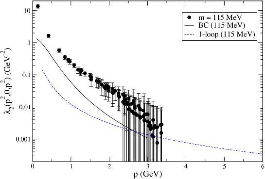
Figure 3: The renormalised form factor $\lambda_{2}(p^{2},0,p^{2})$ as a function of $p$. Also shown is the abelian (Ball–Chiu) form of (9) and the one-loop form of (19).

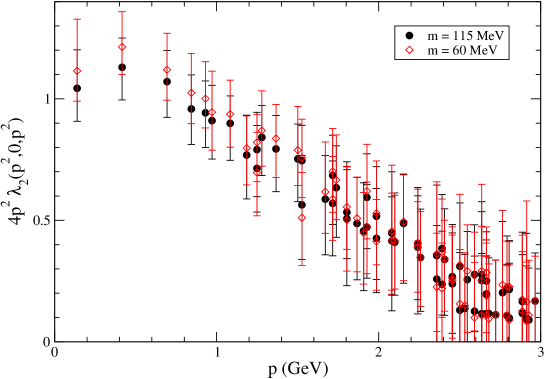
Figure 4: The renormalised form factor $4p^{2}\lambda_{2}(p^{2},0,p^{2})$ as a function of $p$.

This quantity measures the relative strength of this component compared to the tree-level $\lambda_{1}$. We see that $\lambda_{2}$ becomes comparable in strength to $\lambda_{1}$ for the most infrared points.

In figure 5 we show $\lambda_{3}(p^{2},0,p^{2})$ as a function of $p$. Here we have performed a ‘cylinder cut’ [17] with radius 1 unit of spatial momentum to select data close to the 4-dimensional diagonal. We see that it coincides within errors with the Ball–Chiu form (9), and approaches the one-loop form at about 2 GeV. We also see that the quark mass dependence of both $\lambda_{2}$ and $\lambda_{3}$ is very weak.

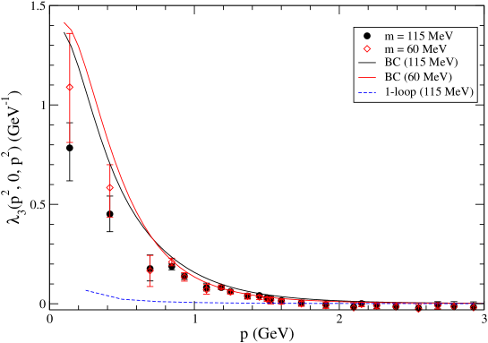
Figure 5: The renormalised form factor $\lambda_{3}(p^{2},0,p^{2})$ as a function of $p$. Also shown is the abelian (Ball–Chiu) form of (9) and the one-loop form of (20).

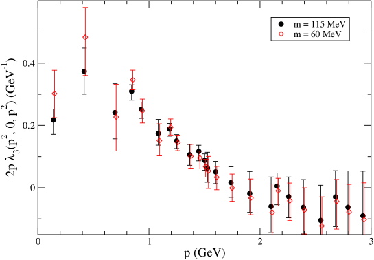
Figure 6: The renormalised form factor $\lambda_{3}(p^{2},0,p^{2})$ multiplied by twice the quark momentum $2p$, as a function of $p$, for $m=115$ MeV. This dimensionless quantity gives a measure of the relative strength of $\lambda_{3}$.

$\lambda_{3}$ becomes somewhat larger as the quark mass is decreased, which corresponds to the effect of dynamical chiral symmetry breaking being relatively larger for a smaller bare mass.

In figure 6 we show $2p\lambda_{3}(p^{2},0,p^{2})$ as a function of $p$. This quantity is dimensionless and measures the relative strength of $\lambda_{3}$ compared to the tree-level $\lambda_{1}$. For the most infrared points, $\lambda_{3}$ can also be seen to contribute significantly to the interaction strength, although clearly not as strongly as $\lambda_{1}$ and $\lambda_{2}$.

In order to see more clearly the relative strength of all three components of the vertex, in figure 7 we show the dimensionless quantities $\lambda_{1},4p^{2}\lambda_{2}$ and $2p\lambda_{3}$ for the heavier quark mass. In this figure, the hierarchy of strengths $\lambda_{1}>\lambda_{2}>\lambda_{3}$ is evident.

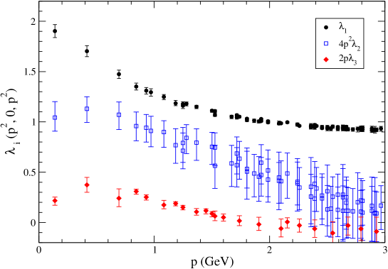
Figure 7: The dimensionless form factors $\lambda_{1},4p^{2}\lambda_{2}$ and $2p\lambda_{3}$ at the asymmetric point, as a function of $p$, for $m=115$ MeV.

4 Symmetric point

Since we have already established that the dependence of the vertex on the quark mass is very weak, in this section we will only be using one quark mass, $m\approx 115$ MeV. We will also in this section make use of the lattice momentum variables $K(p)\equiv\sin(pa)/a$ and $Q(q)\equiv 2\sin(qa/2)/a=-2K(p)$. These momentum variables appear in the lattice tree-level expressions for the form factors we will be studying, as well as in the transverse projector, and are thus appropriate variables to use.

In figure 8, we show $\lambda^{\prime}_{1}$ at the symmetric point as a function of $|Q(q)|$. In contrast to in [6], the tree-level correction here has been carried out on each Lorentz component of the vertex separately, as explained in the Appendix. These results should therefore be more reliable than those shown in [6]. We have also performed a cylinder cut on the data with a radius of 2 units of spatial momentum in $q$. From these data, we determine $1/Z_{1F}^{\overline{\text{MOM}}}(2{\rm GeV},a)=0.95(8)$. Multiplying by $Z_{2}Z_{3}^{1/2}$ determined in [6] we also find $g_{\overline{\text{MOM}}}(2{\rm GeV})=1.47(15)$.

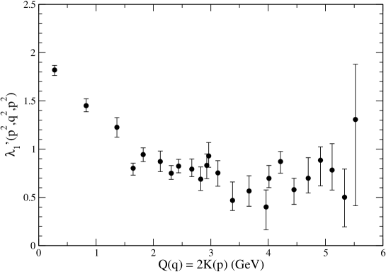
Figure 8: The unrenormalised form factor $\lambda^{\prime}_{1}(p^{2},q^{2},p^{2})$ at the symmetric point $q=-2p$, as a function of the gluon momentum $q$. The data shown are those surviving a cylinder cut with radius 2 units of spatial momentum in $q$.

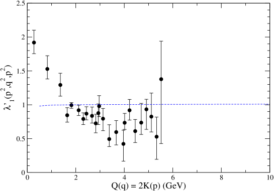
Figure 9: The renormalised form factor $\lambda^{\prime}_{1}(p^{2},q^{2},p^{2})$ at the symmetric point $q=-2p$, as a function of the gluon momentum $q$. Also shown is the one-loop form from [6].

The ratio of renormalisation constants is $Z_{1F}^{\overline{\text{MOM}}}/Z_{1F}^{\overline{\text{MS}}}=1.093$. This is used to determine the one-loop $\lambda^{\prime}_{1}$, shown together with the renormalised lattice $\lambda^{\prime}_{1}$ in figure 9.

In figure 10 we show the form factor $\tau_{5}$ as a function of the gluon momentum $q$. The same cylinder cut has been performed as in fig. 8. We see that, although $\tau_{5}$ is power suppressed in the ultraviolet, it rises very significantly for $q\lesssim 2$ GeV.

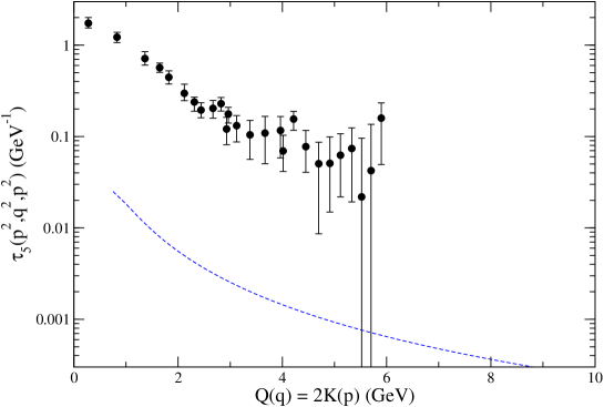
Figure 10: The renormalised form factor $\tau_{5}$ at the symmetric point as a function of the gluon momentum $q$. The data shown are those surviving a cylinder cut with radius 2 units of spatial momentum in $q$. Also shown is the one-loop form of (21).

Although this form factor is related to the chromomagnetic moment, and as such is expected to be of phenomenological importance, it has not previously been included in QED-inspired model vertices commonly used in, e.g., DSE-based studies. However, work is in progress to provide an analytical, nonperturbative expression for this and the other form factors in the purely transverse part of the vertex [18]. We will also compare our lattice results to the one-loop $\tau_{5}$, which in Euclidean space is given by

$$\begin{split}\tau_{5}^{\overline{\text{MS}}}(&s^{2},4s^{2},s^{2})=\frac{g^{2}}{16\pi^{2}}\frac{m}{12s^{2}}\Biggl{\{}(1-\xi)\Bigl{[}8C_{F}+\xi C_{A}-C_{A}\frac{m^{2}(1-\xi)}{s^{2}-m^{2}}\Bigr{]}\\ &-(2C_{F}-C_{A})\frac{4s^{2}(1-\xi)}{s^{2}+m^{2}}\biggl{[}\frac{1}{2}\sqrt{1+\frac{m^{2}}{s^{2}}}\ln\frac{\sqrt{1+\frac{m^{2}}{s^{2}}}+1}{\sqrt{1+\frac{m^{2}}{s^{2}}}-1}+\frac{1}{2}\ln\frac{m^{2}}{\mu^{2}}\biggr{]}\\ &+C_{A}\frac{s^{2}}{s^{2}-m^{2}}\biggl{[}7+9\xi+2\xi^{2}-\frac{2m^{2}(1-\xi)}{s^{2}-m^{2}}\Bigl{(}6-\xi+\frac{2m^{2}(1-\xi)}{s^{2}-m^{2}}\Bigr{)}\biggr{]}\ln\frac{4s^{2}}{\mu^{2}}\\ &+\biggl{[}4C_{F}(1-\xi)\frac{s^{2}-2m^{2}}{s^{2}+m^{2}}-C_{A}\Bigl{(}9+7\xi+2\xi^{2}-\frac{6m^{2}(1-\xi)}{s^{2}+m^{2}}\\ &\phantom{+\biggl{[}4C_{F}}-(6-16\xi+\xi^{2})\frac{2m^{2}}{s^{2}-m^{2}}-\frac{2m^{4}(1-\xi)}{(s^{2}-m^{2})^{2}}\bigl{[}9-4\xi+\frac{2m^{2}(1-\xi)}{s^{2}-m^{2}}\bigr{]}\Bigr{)}\biggr{]}\times\\ &\qquad\times\biggl{[}\ln\frac{s^{2}+m^{2}}{\mu^{2}}+\frac{m^{2}}{s^{2}}\ln\Bigl{(}1+\frac{s^{2}}{m^{2}}\Bigr{)}\biggr{]}\Biggr{\}}\,.\end{split}$$ (21)

We find that the nonperturbative $\tau_{5}$ is several orders of magnitude larger than the one-loop form, and there is no sign of the lattice data approaching the perturbative form even for the most ultraviolet points we can trust, around 5 GeV. We take this as an indication that very strong nonperturbative effects affect this form factor. It is also worth noting that the one-loop contribution to both $\tau_{5}$ and $\lambda^{\prime}_{1}$ at the symmetric point are an order of magnitude smaller than the one-loop contributions to form factors at the asymmetric point.

In order to get a dimensionless measure of the strength of this component relative to the tree-level vertex, we have scaled $\tau_{5}$ with the gluon momentum $q$. We show this together with $\lambda^{\prime}_{1}$ in figure 11. As we can see, between 1 and 2 GeV, $\tau_{5}$ contributes with about the same strength as $\lambda^{\prime}_{1}$, making it a very significant contribution that cannot be ignored.

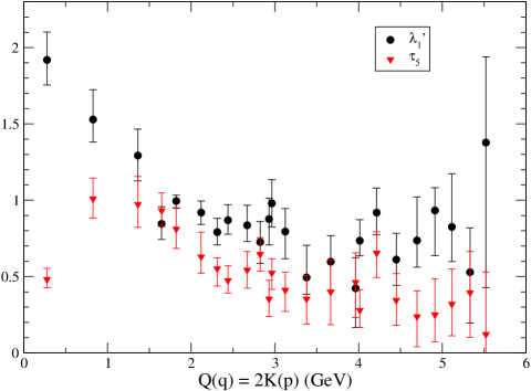
Figure 11: The dimensionless form factors $\lambda^{\prime}_{1}$ and $q\tau_{5}$ at the symmetric point, as a function of $q$. These quantities gives a measure of the relative strength of the two components of the vertex.

Although $\tau_{5}$ has the same tensor structure as the (chromo-)magnetic moment, the relation between the two is not straightforward. In particular, since quarks are never on-shell, the Gordon decomposition which is used to define the magnetic moment in QED is not applicable, making the definition of the chromomagnetic moment ambiguous. This is an issue that deserves further investigation.

5 Outlook

We have computed the complete quark–gluon vertex at two kinematical points, finding substantial deviations from the abelian form — which cannot be described by a universal function multiplying the abelian form as in [9]. This, and the fact that we observe a $p$-dependent enhancement of $\lambda_{1}$ at the asymmetric point, where $q$ and thereby also the ghost form factor $G(q^{2})$ is fixed, indicates that the ghost–quark scattering kernel entering into the Slavnov–Taylor identity (1) must contain nontrivial structure.

The form factor $\tau_{5}$, related to the chromomagnetic moment, has been estimated nonperturbatively for the first time, and found to be important. The work has been carried out on a relatively small lattice, using a fermion discretisation which has serious discretisation errors at large momenta. It will be important to repeat this study using larger lattices and a more well-behaved fermion discretisation.

A natural extension of this work would be to map out the entire kinematical space in the three variables $p^{2},k^{2},q^{2}$. This is numerically very demanding, but work is underway on a complete determination of $\lambda^{\prime}_{1}(p^{2},q^{2},k^{2})$.

Finally, it should be noted that the lattice Landau gauge restricts us to computing only the transverse-projected vertex away from $q=0$; i.e., it is not possible to determine $\lambda_{i},\tau_{i},i=1,\ldots,4$ separately; only the linear combinations $\lambda^{\prime}_{i}$. Although the vertex is always contracted with the gluon propagator in all actual applications, and thus only the transverse-projected vertex plays any role in Landau gauge, it would be of interest to determine all these form factors by computing the vertex in a general covariant gauge — which would also give a handle on the important issue of gauge dependence.

Appendix A Tree-level expressions

The tree-level lattice expressions are given in terms of the lattice momentum variables,

$$K_{\mu}(p) \equiv\frac{1}{a}\sin(p_{\mu}a)\,;$$ (22)

$$Q_{\mu}(p) \equiv\frac{2}{a}\sin(p_{\mu}a/2)=\frac{\sqrt{2}}{a}\sqrt{1-\cos(p_{\mu}a)}\,;$$ (23)

$$\widetilde{K}_{\mu}(p) \equiv\frac{1}{2}K_{\mu}(2p)=\frac{1}{2a}\sin(2p_{\mu}a)\,;$$ (24)

$$C_{\mu}(p) \equiv\cos(p_{\mu}a)\,.$$ (25)

The tree-level vertex is [6]

$$\Lambda^{a(0)}_{I,\mu}(p,q)=c_{m}S_{I}^{(0)}(p)^{-1}S_{0}^{(0)}(p)\Lambda^{a(0)}_{0,\mu}(p,q)S_{0}^{(0)}(p+q)S_{I}^{(0)}(p+q)^{-1}\,,$$ (26)

and

$$(S_{I}^{(0)})^{-1}S_{0}^{(0)} =\frac{1}{D_{I}}\Bigl{(}i\not\!KA_{V}+B_{V}\Bigr{)}\,,$$ (27)

where we have written

$$c_{m} \equiv 1+b_{q}m\,;$$ (28)

$$A_{V}(p) =2c^{\prime}_{q}D(p)\,;$$ (29)

$$B_{V}(p) =(c_{m}-2c^{\prime}_{q}M(p))D(p)\,;$$ (30)

$$D_{I}(p) =\bigl{[}A_{V}^{2}(p)K^{2}(p)+B_{V}^{2}(p)\bigr{]}/D(p)\,;$$ (31)

$$D(p) =K^{2}(p)+M^{2}(p)\,;$$ (32)

$$M(p) =m+\frac{1}{2}Q^{2}(p)\,.$$ (33)

At $q=0$ we have

$$\Lambda^{a(0)}_{I,\mu}(p,0)=\frac{-ig_{0}}{D_{I}^{2}}\Bigl{(}i\not\!KA_{V}(p)+B_{V}(p)\Bigr{)}\Bigl{(}\gamma_{\mu}C_{\mu}(p)-iK_{\mu}(p)\Bigr{)}\Bigl{(}i\not\!KA_{V}(p)+B_{V}(p)\Bigr{)}\,.$$ (34)

This expands to

$$\begin{split}\Bigl{(}i\not\!K&A_{V}+B_{V}\Bigr{)}\Bigl{(}\gamma_{\mu}C_{\mu}-iK_{\mu}\Bigr{)}\Bigl{(}i\not\!KA_{V}+B_{V}\Bigr{)}\\ =&(A_{V}^{2}K^{2}+B_{V}^{2})\gamma_{\mu}C_{\mu}-2A_{V}^{2}C_{\mu}\not\!KK_{\mu}+2iA_{V}B_{V}K_{\mu}C_{\mu}\\ &-iB_{V}^{2}K_{\mu}+2A_{V}B_{V}\not\!KK_{\mu}+iA_{V}^{2}K^{2}K_{\mu}\\ =&(A_{V}^{2}K^{2}+B_{V}^{2})C_{\mu}\gamma_{\mu}+2(A_{V}B_{V}-A_{V}^{2}C_{\mu})\not\!KK_{\mu}\\ &+i(2A_{V}B_{V}C_{\mu}+A_{V}^{2}K^{2}-B_{V}^{2})K_{\mu}\,.\end{split}$$ (35)

The tree-level form factors $\lambda_{2}^{(0)},\lambda_{3}^{(0)}$ can be read off directly:

$$\lambda_{2}^{(0)}+\tilde{\lambda}_{2}^{(0)}C_{\mu} =\frac{c_{m}}{2D_{I}^{2}}\Bigl{(}A_{V}B_{V}-A_{V}^{2}C_{\mu}\Bigr{)}=c_{m}c^{\prime}_{q}\frac{D^{2}}{D_{I}^{2}}\Bigl{[}c_{m}-2c^{\prime}_{q}M-2c^{\prime}_{q}C_{\mu}\Bigr{]}\,;$$ (36)

$$\lambda_{3}^{(0)}+\tilde{\lambda}_{3}^{(0)}C_{\mu} =\frac{c_{m}}{2D_{I}^{2}}\Bigl{(}A_{V}^{2}K^{2}-B_{V}^{2}+2A_{V}B_{V}C_{\mu}\Bigr{)}\,.$$ (37)

The lattice, tree-level corrected equivalents of (13) and (10), which we use to obtain $\lambda_{2}$ and $\lambda_{3}$, are thus

$$\begin{split}\lambda_{2}(p^{2},0,p^{2})&=\frac{1}{4K^{2}(p)}\sum_{\mu}\biggl{[}\frac{1}{4g_{0}}\operatorname{Im}\operatorname{Tr}\gamma_{\mu}\Lambda_{\mu}(p,0)+\lambda_{1}(p^{2},0,p^{2})\\ &\phantom{=\frac{1}{4K^{2}(p)}\sum_{\mu}\biggl{[}}-4K_{\mu}^{2}(p)\Bigl{(}\lambda_{2}^{(0)}(p)+\tilde{\lambda}_{2}^{(0)}(p)C_{\mu}(p)\Bigl{)}\biggr{]}\,;\end{split}$$ (38)

$$\lambda_{3}(p^{2},0,p^{2}) =\frac{1}{2K^{2}(p)}\sum_{\mu}\biggl{[}K_{\mu}(p)\frac{1}{4g_{0}}\operatorname{Re}\operatorname{Tr}\Lambda_{\mu}(p,0)-2K_{\mu}^{2}(p)\Bigl{(}\lambda_{3}^{(0)}(p)+\tilde{\lambda}_{3}^{(0)}(p)C_{\mu}(p)\Bigr{)}\biggr{]}\,.$$ (39)

The tree-level vertex at the symmetric point is given by eq. (B.21) of [6]. We use the following decomposition into independently transverse tensors,

$$\begin{split}\frac{i}{g_{0}}\Lambda^{(0)}_{I,\mu}(p,-2p)=&\lambda_{1}^{(0)}\gamma_{\mu}-\tau_{3}^{(0)}(Q^{2}\gamma_{\mu}-\not\!QQ_{\mu})-\tilde{\tau}_{3}^{(0)}(K\!\cdot\!QC_{\mu}\gamma_{\mu}-\not\!KK_{\mu})\\ &-i\tau_{5}^{(0)}\sum_{\nu}\sigma_{\mu\nu}Q_{\nu}-i\tilde{\tau}_{5}^{(0)}C_{\mu}\sum_{\nu}\sigma_{\mu\nu}K_{\nu}\\ &-i\tilde{\tau^{\prime}}_{5}^{(0)}\Bigl{[}C_{\mu}\sum_{\nu}\sigma_{\mu\nu}Q_{\nu}+K_{\mu}\sum_{\nu\lambda}\sigma_{\nu\lambda}Q_{\nu}K_{\lambda}/(Q\cdot K)\Bigr{]}\,,\end{split}$$ (40)

where $Q\equiv Q(q),K\equiv K(q),C\equiv C(q/2)$; $\lambda_{1}^{(0)},\tau_{3}^{(0)}$ and $\tilde{\tau}_{3}^{(0)}$ are given by (B.25)–(B.27) of [6], and

$$\tau_{5}^{(0)} =\frac{c_{m}}{D_{I}^{2}}{A_{V}(p)B_{V}(p)}=2c_{m}c^{\prime}_{q}(c_{m}-2c^{\prime}_{q}M(p))\frac{D^{2}(p)}{D_{I}^{2}(p)}\,;$$ (41)

$$\tilde{\tau}_{5}^{(0)} =-\frac{c_{\text{sw}}c_{m}}{2}\frac{D(p)}{D_{I}(p)}\,;$$ (42)

$$\tilde{\tau^{\prime}}_{5}^{(0)} =c_{\text{sw}}c_{m}\frac{A_{V}^{2}(p)(K(p)\cdot\widetilde{K}(p))}{D_{I}^{2}(p)}=4c_{\text{sw}}c_{m}{c^{\prime}_{q}}^{2}(K(p)\cdot\widetilde{K}(p))\frac{D^{2}(p)}{D_{I}^{2}(p)}\,.$$ (43)

Since the continuum $\lambda^{\prime}_{1}(\gamma_{\mu}-\not\!qq_{\mu}/q^{2})$ becomes two independent tensors on the lattice,

$$\lambda^{\prime}_{1}\left(\frac{q^{2}}{4},q^{2},\frac{q^{2}}{4}\right)\left(\gamma_{\mu}-\frac{\not\!qq_{\mu}}{q^{2}}\right)\to(\lambda_{1}-Q^{2}\tau_{3})\left(\gamma_{\mu}-\frac{\not\!QQ_{\mu}}{Q^{2}}\right)-\tilde{\tau}_{3}(K\!\cdot\!QC_{\mu}\gamma_{\mu}-\not\!KK_{\mu})\,,$$ (44)

we cannot simply factor out the tree-level behaviour with a simple multiplicative correction. Instead we apply a ‘hybrid’ scheme where the dominant term, multiplying $(\gamma_{\mu}-\not\!QQ_{\mu}/Q^{2})$, is corrected multiplicatively, after first subtracting off the remaining part,

$$\tilde{\tau}_{3}^{(0)}\Bigl{[}(K\!\cdot\!QC_{\mu}\gamma_{\mu}-\not\!KK_{\mu})-K\!\cdot\!QC_{\mu}(\gamma_{\mu}-\not\!QQ_{\mu}/Q^{2})\Bigr{]}=-\tilde{\tau}_{3}^{(0)}\Bigl{(}K_{\mu}^{2}-K_{\mu}Q_{\mu}\frac{K\!\cdot\!Q}{Q^{2}}\Bigr{)}\,.$$ (45)

It turns out that this term is completely negligible, but it has still been included in the correction. Thus, the lattice, tree-level corrected equivalent of (12) which we use to compute $\lambda^{\prime}_{1}$, is

$$\lambda^{\prime}_{1}\left(\frac{q^{2}}{4},q^{2},\frac{q^{2}}{4}\right)= \frac{1}{3}\sum_{\mu}\frac{-\frac{1}{4g_{0}}\operatorname{Im}\operatorname{Tr}\gamma_{\mu}\Lambda^{P}_{\mu}(-q/2,q)-\tilde{\tau}_{3}^{(0)}\Bigl{(}K_{\mu}^{2}-K_{\mu}Q_{\mu}\frac{K\!\cdot\!Q}{Q^{2}}\Bigr{)}}{\lambda_{1}^{(0)}-Q^{2}\tau_{3}^{(0)}-K\!\cdot\!Q\tilde{\tau}_{3}^{(0)}C_{\mu}}\,.$$ (46)

For $\tau_{5}$ we employ an additive correction scheme, and thus the lattice equivalent of (11) is

$$\begin{split}\tau_{5}\left(\frac{q^{2}}{4},q^{2},\frac{q^{2}}{4}\right)=&-\frac{1}{3Q^{2}(q)}\sum_{\mu,\nu}\biggl{[}Q_{\mu}(q)\frac{1}{4g_{0}}\operatorname{Re}\operatorname{Tr}\sigma_{\mu\nu}\Lambda^{P}_{\nu}(-q/2,q)\\ &-Q_{\mu}^{2}\Bigl{\{}\tau_{5}^{(0)}+C_{\mu}C_{\nu}\tilde{\tau}_{5}^{(0)}+C_{\nu}\tilde{\tau^{\prime}}_{5}^{(0)}\bigl{[}1-(C_{\nu}-C_{\mu})Q_{\nu}^{2}/Q\cdot\!\!K\bigr{]}\Bigr{\}}\biggr{]}\,.\end{split}$$ (47)

References

[1]
A. I. Davydychev, P. Osland and L. Saks, Quark gluon vertex in arbitrary
gauge and dimension, Phys. Rev.D63 (2001) 014022
[hep-ph/0008171].
[2]
K. G. Chetyrkin and A. Rétey, Three-loop three-linear vertices and
four-loop functions in massless QCD,
hep-ph/0007088.
[3]
K. G. Chetyrkin and T. Seidensticker, Two loop QCD vertices and three
loop MOM functions, Phys. Lett.B495 (2000) 74–80
[hep-ph/0008094].
[4]
J. I. Skullerud, Renormalisation in lattice QCD.
PhD thesis, University of Edinburgh, 1996.
[5]UKQCD Collaboration, J. I. Skullerud, The running coupling from the
quark gluon vertex, Nucl. Phys. Proc. Suppl.63 (1998) 242
[hep-lat/9710044].
[6]
J. Skullerud and A. Kızılersü, Quark-gluon vertex from lattice
QCD, JHEP09 (2002) 013
[hep-ph/0205318].
[7]
L. von Smekal, A. Hauck and R. Alkofer, A solution to coupled
Dyson-Schwinger equations for gluons and ghosts in Landau gauge, Ann. Phys.267 (1998) 1
[hep-ph/9707327].
[8]
D. Atkinson and J. C. R. Bloch, Running coupling in non-perturbative
QCD. I: Bare vertices and y-max approximation, Phys. Rev.D58 (1998) 094036 [hep-ph/9712459].
[9]
C. S. Fischer and R. Alkofer, Non-perturbative propagators, running
coupling and dynamical quark mass of Landau gauge QCD,
hep-ph/0301094.
[10]UKQCD Collaboration, D. B. Leinweber, J. I. Skullerud, A. G. Williams and
C. Parrinello, Asymptotic scaling and infrared behavior of the gluon
propagator, Phys. Rev.D60 (1999) 094507
[hep-lat/9811027].
[11]
F. D. R. Bonnet, P. O. Bowman, D. B. Leinweber and A. G. Williams, Infrared behavior of the gluon propagator on a large volume lattice, Phys. Rev.D62 (2000) 051501
[hep-lat/0002020].
[12]
F. D. R. Bonnet, P. O. Bowman, D. B. Leinweber, A. G. Williams and J. M.
Zanotti, Infinite volume and continuum limits of the Landau-gauge
gluon propagator, Phys. Rev.D64 (2001) 034501
[hep-lat/0101013].
[13]
J. Skullerud, P. Bowman and A. Kızılersü, The nonperturbative
quark gluon vertex, hep-lat/0212011.
[14]
J. C. R. Bloch, A. Cucchieri, K. Langfeld and T. Mendes, Running coupling
constant and propagators in SU(2) Landau gauge,
hep-lat/0209040.
[15]
J. Skullerud, D. B. Leinweber and A. G. Williams, Nonperturbative
improvement and tree-level correction of the quark propagator, Phys.
Rev.D64 (2001) 074508
[hep-lat/0102013].
[16]
P. O. Bowman, U. M. Heller, D. B. Leinweber and A. G. Williams, Modelling
the quark propagator, hep-lat/0209129.
[17]UKQCD Collaboration, D. B. Leinweber, J. I. Skullerud, A. G. Williams and
C. Parrinello, Gluon propagator in the infrared region, Phys.
Rev.D58 (1998) 031501
[hep-lat/9803015].
[18]
A. Kızılersü and M. R. Pennington, “Building the full fermion-boson
vertex of QED by imposing the multiplicative renormalizability of the
Schwinger-Dyson equations for the fermion and boson propagators.” In
preparation, 2003.