arXiv:hep-ph/yymmnn

UFIFT-HEP-02-24

CRETE-02-13

POST–INFLATIONARY DYNAMICS

N. C. Tsamis^†

Department of Physics, University of Crete
GR-710 03 Heraklion, HELLAS.

R. P. Woodard^‡

Department of Physics, University of Florida
Gainesville, FL 32611, UNITED STATES.

ABSTRACT

We argue that $\Lambda$-driven inflation must overshoot into an era of deflation. The deflationary period ends quickly with the creation of a hot dense thermal barrier to the forward propagation of quantum correlations from the period of inflationary particle production. Subsequent evolution is controlled by the balance between the persistence of this barrier and the growth in the 4-volume from which such correlations can be seen. This balance can lead to power law expansion.

PACS numbers: 11.15.Kc, 12.20-m

^† e-mail: tsamis@physics.uoc.gr

^‡ e-mail: woodard@phys.ufl.edu

1 Introduction

Although it is not obvious how to account for the recent supernovae data [1], it is by now quite clear that an adequate period of approximately exponential expansion – inflation [2] – provides a simple and natural explanation for the homogeneity and isotropy of the large-scale observable universe [3]. The explicit realization of this inflationary phase is usually done by a scalar field but this is not necessary.

Consider the effective four-dimensional gravitational theory that emerges from the full – and yet unknown – quantum gravitational theory when we restrict physical processes to scales well below the Planck scale. It is governed, among other things, by general coordinate invariance and can be written as a series of local terms of increasing dimensionality in the curvature. Of these terms, only the lowest dimensionality ones are relevant in the range of scales of interest: the cosmological constant and the Ricci scalar. On the quantum level this effective theory is not renormalizable but, nonetheless, is BPHZ renormalizable:

$${\cal L_{\rm GR}}={1\over 16\pi G}\Bigl{(}-2\Lambda+R\;\Bigr{)}\;\sqrt{-g}\;+\;{\rm(counterterms)}\;.$$ (1)

Each of the BPHZ counterterms contains an infinite and a finite part. The infinite parts are fixed by having to absorb the ultraviolet divergences that are generated order by order. Of the finite parts, only the lowest dimensionality ones are known and are fixed from the measured values of the expansion rate for $\Lambda$ and the Newtonian force for $G$. All the remaining finite parts are unknown and can only be determined from the full theory. However, since cosmology is determined by the infrared sector of the theory – where only the lowest dimensionality finite parts dominate – it is insensitive to these unknown parts.

In the above gravitational effective theory and if $\Lambda$ is assumed to be positive, the “no-hair” theorems imply that – classically – the local geometry approaches the maximally symmetric solution at late times [4]. This solution is de Sitter spacetime and, thus, $\Lambda$-driven inflation is intrinsic to (1) and commences naturally in a way that scalar-driven inflation cannot. As long as the matter stress-energy is finite and obeys the weak energy condition, pre-inflationary expansion redshifts the initial matter stress-energy until it is dominated by the cosmological constant $\Lambda>0$. By contrast, scalar-driven inflation is triggered by a random field fluctuation which must be homogeneous over more than a Hubble volume [5]. This condition is so unlikely that it has not happened even once in the observed history of the universe.

What is hard to realize is how $\Lambda$-driven inflation can ever stop. In Section 2, we review perturbative results from the inflationary regime [6]. The main conclusion is that long-range correlations from inflationary infrared graviton production build-up and screen the observed expansion rate. While it is the graviton that is involved in the physical case, we shall use – solely for reasons of quantitative simplicity – a model based on a self-interacting massless minimally coupled scalar which is fine-tuned to mimic most of the essential properties of the graviton.

In Section 3, we argue that this screening effect inevitably results in a period of deflation. Stability would forbid any recovery on the classical level. However, the quantum universe is driven back to expansion because deflation compresses the most recently produced infrared particles during inflation into a hot, dense “thermal barrier” . This barrier degrades correlations from the inflationary period by scattering the infrared quanta that carry these correlations and, hence, depleting the number of such quanta.

Section 4, addresses the post-deflationary evolution of the universe. Under the assumption that the barrier actually becomes thermal, it is shown that the asymptotic geometry can be that of a small power law expanding universe. Our conclusions comprise Section 5.

2 The Inflationary Regime

(i) Basics
The effective theory defined by (1) is studied in the presence of homogeneous and isotropic backgrounds:

$$ds^{2} = -dt^{2}+a^{2}(t)\;d{\vec{x}}\cdot d{\vec{x}}\;=\;-dt^{2}+\exp\left[\,2\,b(t)\,\right]\;d{\vec{x}}\cdot d{\vec{x}}\;\;,$$ (2)

$$= {\it\Omega}^{2}(\eta)\;\Bigl{(}-d\eta^{2}+d{\vec{x}}\cdot d{\vec{x}}\Bigr{)}\;\;,$$ (3)

where we have expressed the line element both in co-moving and conformal coordinates. The theory is valid as long as we restrict physics to scales below the Planck mass or, equivalently, as long as its dimensionless coupling constant is small:

$$M\equiv\Bigl{(}{\Lambda\over{8\pi G}}\Bigr{)}^{\frac{1}{4}}<M_{\rm Pl}\quad\iff\quad G\Lambda<1\;\;.$$ (4)

This is a quite wide range of scales; for instance, if $M\sim 10^{16}GeV$ we get that $G\Lambda\sim 10^{-12}$.

Let $\gamma_{\mu\nu}(t,{\vec{x}})$ stand for the metric operator. We shall be interested in quantum corrections to the classical background geometry:

$$\left\langle\,state\,\left|\;\gamma_{\mu\nu}(t,{\vec{x}})\;dx^{\mu}dx^{\nu}\;\right|\,state\,\right\rangle\;=\;g_{\mu\nu}(t,{\vec{x}})\;dx^{\mu}dx^{\nu}\;\;.$$ (5)

Geometrically significant differences between the classical and quantum backgrounds can be ascribed to a quantum-induced stress tensor. This is defined from the deficit by which the quantum background $g_{\mu\nu}$ fails to obey the classical equations of motion:

$$8\pi G\;T_{\mu\nu}\equiv R_{\mu\nu}-\frac{1}{2}g_{\mu\nu}R+g_{\mu\nu}\Lambda\;\;.$$ (6)

In (6) $R_{\mu\nu}$ and $R$ are the Ricci tensor and Ricci scalar constructed from the quantum background $g_{\mu\nu}$. The structure of the induced stress tensor is dictated by homogeneity and isotropy:

$$T_{00}(t)\ =\ -\rho(t)\;g_{00}\quad,\quad T_{0i}(t)\ =\ 0\quad,\quad T_{ij}(t)\ =\ p(t)\;g_{ij}\;\;,$$ (7)

where $\rho(t)$ is the induced energy density and $p(t)$ the induced pressure. The latter obey:

$$\rho(t) = {1\over 8\pi G}\left[\,\dot{b}^{2}(t)-\Lambda\,\right]\;\;,$$ (8)

$$p(t) = {1\over 8\pi G}\left[\,-2\ddot{b}(t)\,\right]-\rho(t)\;\;.$$ (9)

An observable which measures the expansion rate of the universe is the effective Hubble parameter:

$$H(t)\equiv{{\dot{a}}(t)\over a(t)}={\dot{b}}(t)=\frac{{\it\Omega}^{\prime}(\eta)}{{\it\Omega}^{2}(\eta)}=\sqrt{\,\frac{\Lambda}{3}+\frac{8\pi G}{3}\rho(t)}\;\;.$$ (10)

(ii) Results During Inflation
According to [4], time evolution from generic initial value data leads to a locally de Sitter background:

$$a_{dS}(t)=\exp\left[\,b_{dS}(t)\,\right]=e^{Ht}=\,{\it\Omega}_{dS}(\eta)=-\frac{1}{H\eta}\;\;,$$ (11)

where the Hubble constant $H$ is defined as:

$$H^{2}\equiv\frac{1}{3}\Lambda>0\;\;.$$ (12)

It is quite unlikely for inflation to have started simultaneously over a region larger than a causal volume. Hence, we shall consider (11) on the manifold $T^{3}\times\Re$, with the physical distances of the toroidal radii equal to a Hubble length at the onset of inflation:

$$-\frac{1}{2}H^{-1}<x^{i}\leq\frac{1}{2}H^{-1}\;\;.$$ (13)

The onset of inflation is taken to be at $t=0$:

$$b_{dS}(0)=0\quad,\quad{\dot{b}}_{dS}(0)=H\;\;,$$ (14)

$$\Big{|}\,state\Big{\rangle}=\Big{|}\;{\rm Bunch\;Davies\;vacuum\;at}\;t=0\;\Big{\rangle}\equiv\Big{|}\hskip 1.42271pt0\Big{\rangle}\;\;.$$ (15)

Time evolution is determined from the dynamics of the theory. Concrete results have been obtained in a perturbation theory organized in terms of the fluctuating field $\psi_{\mu\nu}(x)$:

$$\gamma_{\mu\nu}\equiv\;{\it\Omega}^{2}\left(\eta_{\mu\nu}+\kappa\,\psi_{\mu\nu}\right)\quad,\quad\kappa^{2}\equiv 16\pi G\;\;,$$ (16)

and in the infrared limit of a large number of inflationary e-foldings. For the background (11), the map between the relevant co-moving and conformal time intervals obeys:

$$t\in\left[\;0\;,\;+\infty\right)\quad\iff\quad\eta\in\left[-H^{-1}\;,\;0^{-}\right)\;\;.$$ (17)

In terms of the dimensionless coupling constant $\varepsilon$ of the theory:

$$\varepsilon\equiv{G\Lambda\over 3\pi}=\left({\kappa H\over 4\pi}\right)^{2}={8\over 3}\left({M\over M_{\rm Pl}}\right)^{4}\;\;,$$ (18)

the leading infrared results to the first non-trivial order of perturbation theory are [6]:

$$\rho_{dS}(t) = -\varepsilon H^{4}\left[\;\frac{1}{8\pi^{2}}\;(Ht)^{2}\;+\;O(Ht)\;\right]+\;O(\varepsilon^{2})\;\;,$$ (19)

$$p_{dS}(t) = \varepsilon H^{4}\left[\;\frac{1}{8\pi^{2}}\;(Ht)^{2}\;+\;O(Ht)\;\right]+\;O(\varepsilon^{2})\;\;,$$ (20)

$$H_{dS}(t) = H\left\{1-\varepsilon^{2}\left[\;\frac{1}{6}\;(Ht)^{2}\;+\;O(Ht)\;\right]+\;O(\varepsilon^{3})\right\}\;\;.$$ (21)

The negative sign in (19) and (21) is due to the universal attractive nature of the gravitational interaction. The fact that the induced energy density and pressure obey the equation of state of vacuum energy (19-20) is a simple consequence of stress-energy conservation:

$${\dot{\rho}_{dS}}=-3H\left(\,\rho_{dS}+p_{dS}\right)\;\;,$$ (22)

and the inherent weakness of the gravitational interaction for scales $M$ below the Planck mass. This implies that $\rho_{dS}$ changes much slower than the expansion rate, and hence:

$$|{\dot{\rho}_{dS}}(t)|\;\ll\;H\;|\rho_{dS}(t)|\quad\Longrightarrow\quad p_{dS}(t)\;\sim\;-\rho_{dS}(t)\;\;.$$ (23)

It becomes apparent from (21) that the rate of expansion decreases by an amount which becomes non-perturbatively large at late times. This occurs when the effective coupling constant becomes of order one and gives a rough estimate for the number of inflationary e-foldings:

$$\varepsilon\;Ht_{1}\sim 1\quad\Longrightarrow\quad Ht_{1}\sim\left({M_{\rm Pl}\over M}\right)^{4}\;\;.$$ (24)

The higher order perturbative effects make a phenomenologically insignificant correction of the rough estimate for $N_{1}$ [7]:

$$N_{1}\equiv Ht_{1}\sim\left({M_{\rm Pl}\over M}\right)^{\frac{8}{3}}\quad\Longrightarrow\quad N_{1}\gg 60\;\;.$$ (25)

For any acceptable scale $M$, (25) trivially satisfies the bound imposed by the causality problem that inflationary cosmology must solve: $N_{1}\gg 60$. Thus, $\Lambda$-driven inflation persists over many e-foldings for the simple reason that gravity is a weak interaction.

Moreover, the perturbative results can be used to show that inflation ends suddenly over the course of very few e-foldings [7] and, therefore, subsequent reheating becomes possible. Finally, the same results allow the computation of the spectrum of cosmological density perturbations [8] which are observational remnants from this epoch.

The very existence of a bare positive cosmological constant in the effective gravitational theory is enough to drive inflation – there is no need to introduce a scalar field and to fine tune $\Lambda$ to zero. The resulting inflationary model depends on the single parameter $G\Lambda$ only and, consequently, it is very predictive and natural. Both of these properties are severely diminished in scalar-driven inflation by the presence of the parameter space of the scalar potential.

The duration of inflation is naturally long since the gravitational processes must take a while to coherently superpose and overcome their inherently weak coupling constant $G\Lambda$. This should be contrasted with scalar-driven inflation, where the scalar potential has to be tuned to be constant over the very extended region that must cover at least 60 inflationary e-foldings. In our case, the bare cosmological constant naturally achieves the same goal since it is a constant.

Similarly, a sudden exit from inflation implies that the scalar potential must be further tuned to have a steep drop after its extended constancy. For $\Lambda$-driven inflation, as we approach the critical number of e-foldings $N_{1}$, the quantum gravitational effect gets strong and quickly screens the bare cosmological constant naturally.

Another requirement for the occurence of scalar-driven inflation, is the presence of a homogeneous fluctuation of the scalar field over more than one Hubble volume [5]. This is very improbable and the issue is altogether avoided when gravity is the driving force.

(iii) Matter Contributions During Inflation
In addition to the pure gravitational sector (1), the effective theory below $M_{\rm Pl}$ contains a matter sector ${\cal L_{\rm M}}$:

$${\cal L}_{\rm TOT}={\cal L_{\rm GR}}+{\cal L_{\rm M}}\;\;.$$ (26)

All matter quanta reside in ${\cal L_{\rm M}}$ and we must study their back-reaction during the inflationary period, just as we did for the graviton. We need only be concerned with effectively massless particles since it is on the infrared limit of late observational times that we focus. This is because infrared effects influence a local observation through the coherent superposition of distant interactions in the past lightcone of the observer. These interactions cannot be transmitted by massive quanta as their propagators oscillate inside the lightcone and, thus, result in destructive interference.

The critical mass scale $m_{1}$ which separates an effectively massless from an effectively massive particle reflects whether the particle induces a strong infrared effect faster or slower respectively with respect to the graviton. An accurate estimate can be obtained by computing the particle mass below or above which the free mode functions of the particle suffer small or large distortions respectively over the relaxation time $t_{1}$ [9]:

$$m_{1}\sim M\left({M_{\rm Pl}\over M}\right)^{\frac{7}{3}}\;\;.$$ (27)

Let us now consider massless quanta. If the interactions of a massless particle have local conformal invariance, then the particle is unaware of the inflating spacetime and cannot induce a back-reaction. This is most transparent in conformal coordinates where any local quantity has the same form as in flat space; the overall effect is nill since the conformal coordinate volume is only $H^{-4}$. Consequently, all effectively massless fermions and gauge bosons need not be considered. The same holds true for conformally coupled effectively massless scalars.

Effectively massless, minimally coupled scalar particles – with or without self-interactions – require closer inspection [10]. Consider such a scalar theory in the presence of the inflationary background (11):

$${\cal L}_{\varphi}=-\frac{1}{2}\sqrt{-g}\;g^{\mu\nu}\;\partial_{\mu}\varphi\;\partial_{\nu}\varphi\;-\;\sqrt{-g}\;V(\varphi)\;\;,$$ (28)

where, for stability reasons, the potential $V(\varphi)$ is to be bounded from below. Let us assume that at $t=0$ the scalar field is at the true minimum of the potential. This minimum need not be identical to the classical minimum as it includes potentially non-trivial ultraviolet corrections. Evolution generates a finite time-dependent part in the vacuum expectation value of the square of the field operator:

$$\left\langle 0\left|\;\varphi^{2}(x)\;\right|0\right\rangle\;\sim\;H^{2}(Ht)\;+\;{\rm(constant\;ultraviolet\;part)}\;\;.$$ (29)

Consequently, the energy of the scalar field increases with time and so does the expansion rate.

As soon as the scalar field moves upwards its potential, the tendency to reverse its motion and lower its energy appears; it results in a decrease of the expansion rate. The two opposing tendencies eventually balance at a constant asymptotic value which has the true minimum as its lower bound. The net effect on the expansion rate is that it cannot decrease from its initial value $H$.

In any case, the physical existence of scalar fields with dynamics based on (28) is hard to justify unless they have a mass of the same order as the scale $M$ of the theory. The purpose of the above argument was to show that, even if they exist and are effectively massless, they cannot diminish the expansion rate of the universe.

Figure 1: First order graviton contributions to: (a) the expansion rate $H(t)$ , (b) its                      mass.

(iv) Graviton-Like Scalar Model
By virtue of its masslessness and lack of conformally invariant interactions, the graviton is the unique known particle which can mediate a non-trivial back-reaction to an inflationary expansion. To follow the evolution beyond the inflationary regime, it is very instructive – before using the exceedingly complicated graviton dynamics – to construct a scalar field theory that simulates the behaviour of the graviton. Since a free graviton has the same dynamics as a massless minimally coupled scalar, it is reasonable to use the latter with a suitable interaction. Although a derivative interaction would perhaps be more appropriate, we shall choose a quartic self-interaction for calculational simplicity:

$${\cal L}_{\varphi}=-\frac{1}{2}\sqrt{-g}\;g^{\mu\nu}\;\partial_{\mu}\varphi\;\partial_{\nu}\varphi\;-\;\frac{1}{4!}\sqrt{-g}\;\lambda\varphi^{4}\;+\;{\rm(counterterms)}\;\;.$$ (30)

There are two basic properties of the graviton we should like the scalar theory to retain to the extent that it can:
– The scalar should induce an infrared effect which reduces the inflationary expansion of spacetime.
– The scalar should stay massless as much as possible.

Neither of these properties are present in (30). The source of the difference resides in the part of the coincidence limit of the propagator that grows linearly with time: in contrast to the scalar, this part does not couple to anything at one loop for the graviton. Hence, there is no first order contribution to $H(t)$ from gravitons [12]. Gravitational infrared contributions to $H(t)$ begin at second order and are a net drag on the expansion rate of the universe [7]. No graviton mass develops at any order. (see Figure 1)

In the scalar field theory (30), there is a first order ultraviolet contribution to $H(t)$ that enhances the expansion of spacetime. Furthermore, to the same order, there is a time dependent scalar mass induced; the mass counterterm can only absorb the constant ultraviolet part of (29). (see Figure 2)

Figure 2: First order scalar contributions to: (a) the expansion rate $H(t)$ , (b) its                      mass.

To achieve the desired correspondence, we must normal order the scalar theory. More precisely, since we operate in curved spacetime, we must covariantly normal order:

$$\colon\varphi^{2}(x)\;\colon\;\equiv\;\varphi^{2}(x)-i\Delta_{g}(x;x)\;\;,$$ (31)

where the subscript $g$ reminds us of the dependence of $\Delta(x;x)$ on the metric $g_{\mu\nu}$. It follows that:

$${\cal L}_{\colon\varphi\colon} \equiv -\ \frac{1}{2}\ \sqrt{-g}\;g^{\mu\nu}\;\colon\partial_{\mu}\varphi\;\partial_{\nu}\varphi\;\colon\;-\;\frac{1}{4!}\sqrt{-g}\;\lambda\;\colon\varphi^{4}\;\colon$$ (33)

$$+\;\;{\rm(counterterms)}\;\;,$$

$$= -\ \frac{1}{2}\ \sqrt{-g}\;g^{\mu\nu}\;\left[\;\partial_{\mu}\varphi\;\partial_{\nu}\varphi\;-\;{\overrightarrow{\partial}_{\mu}}\;i\Delta_{g}(x;x)\;{\overleftarrow{\partial}_{\nu}}\;\right]$$

$$-\ \frac{1}{4!}\ \sqrt{-g}\;\lambda\;\left[\;\varphi^{4}-6i\Delta_{g}(x;x)\;\varphi^{2}+3\left(i\Delta_{g}(x;x)\right)^{2}\;\right]$$

$$+\;\;{\rm(counterterms)}\;\;.$$

In the flat spacetime limit, the above prescription reduces to the usual normal ordering one.

The scalar theory given by (33) is fully well-defined when the metric is non-dynamical. For a dynamical metric, it is only well-defined perturbatively [13]. In (33) there are no more scalar tadpoles. Their elimination automatically implies that there can be no first order expansion enhancing contribution to $H(t)$, and no first order time dependent scalar mass generated. Moreover, the conservation of the scalar stress tensor is preserved because of the covariant nature of the normal ordering prescription.

Figure 3: Second order scalar contributions to the expansion rate $H(t)$.

The first non-trivial contributions to $H(t)$ have been computed [9] and they behave in the desired way by slowing the inflationary expansion (see Figure 3). In fact, for reasonable values of $\lambda$, they do so by an amount which overwhelms the analogous reduction (21) due to the graviton:

$$H^{\colon\varphi\colon}_{dS}(t)=H\left\{1-\frac{\lambda^{2}\,\varepsilon}{2^{7}\,\pi^{4}}\left[\;\frac{1}{3^{3}}\;(Ht)^{4}\;+\;O(H^{3}t^{3})\;\right]+\;O(\lambda^{3})\;\right\}\;\;.$$ (34)

This result should be contrasted with that coming from the scalar field theory (30) which is not covariantly normal ordered [14]:

$$H^{\varphi}_{dS}(t)=H\left\{1+\frac{\lambda\,\varepsilon}{2^{4}\,\pi^{2}}\left[\;\frac{1}{3}\;(Ht)^{2}\;+\;O(Ht)\;\right]+\;O(\lambda^{2})\;\right\}\;\;.$$ (35)

3 Deflation Begins

(i) General Analysis
Inflation is slowed by the quantum gravitational response to the production of infrared gravitons. However, to understand post-inflationary evolution we must develop a manner of thinking about the various physical effects which can be applied for a general scale factor.

Since physical gravitons obey the same equation of motion as massless, minimally coupled scalars, we shall study the Lagrangian density:

$${\cal L}=-\frac{1}{2}\sqrt{-g}\;g^{\mu\nu}\;\partial_{\mu}\varphi\;\partial_{\nu}\varphi\;\;,$$ (36)

on the manifold $T^{3}\times\Re$ with spatial co-moving coordinate range (13). Wave vectors are discrete:

$${\vec{k}}=2\pi H{\vec{n}}\;\;,$$ (37)

and phase space integrals become mode sums:

$$\int\frac{d^{3}k}{(2\pi)^{3}}\;f(\vec{k})\quad\longrightarrow\quad H^{3}\;\sum_{\vec{k}}f(\vec{k})=H^{3}\;\sum_{\vec{n}}f(2\pi H{\vec{n}})\;\;.$$ (38)

The scalar field can be expanded as a spatial Fourier sum:

$$\varphi(\eta,{\vec{x}})\;=\;H^{3}\;\sum_{\vec{k}}\,e^{i{\vec{k}}\cdot{\vec{x}}}\,\,{\widetilde{\varphi}}(\eta,{\vec{k}})\;\;,$$ (39)

and each wave number can be treated separately because the Lagrangian is diagonal in the mode basis:

$$L(\eta) \equiv \int d^{3}x\;\;{\cal L}(\eta,{\vec{x}})$$ (40)

$$= \frac{1}{2}\,H^{3}\,{\it\Omega}^{2}\;\sum_{\vec{k}}\;\left[\,\|\,{\widetilde{\varphi}}^{\prime}(\eta,{\vec{k}})\,\|^{2}\;-\;k^{2}\,\|\,{\widetilde{\varphi}}(\eta,{\vec{k}})\,\|^{2}\,\right]\;\;.$$ (41)

The momentum canonically conjugate to ${\widetilde{\varphi}}(\eta,{\vec{k}})$ is:

$$\pi(\eta,\vec{k})\,\equiv\ H^{3}\,{\it\Omega}^{2}\;{\widetilde{\varphi}}^{\hskip 0.85355pt*}{{}^{\prime}}(\eta,{\vec{k}})\;\;,$$ (42)

resulting in the following generator of conformal time evolution for wave number ${\vec{k}}$ :

$$H(\eta,{\vec{k}}) = {\|\,\pi(\eta,{\vec{k}})\,\|^{2}\over 2H^{3}\,{\it\Omega}^{2}}\,+\,\frac{1}{2}\,H^{3}\,{\it\Omega}^{2}\,k^{2}\,\|\,{\widetilde{\varphi}}(\eta,{\vec{k}})\,\|^{2}$$ (43)

$$= \frac{1}{2}\,H^{3}\,{\it\Omega}^{2}\left[\,\|\,{\widetilde{\varphi}}^{\prime}(\eta,{\vec{k}})\,\|^{2}\;+\;k^{2}\,\|\,{\widetilde{\varphi}}(\eta,{\vec{k}})\,\|^{2}\,\right]$$ (44)

At any instant ${\it\Omega}(\eta)$ is just a number. By comparing (43) with the usual harmonic oscillator of mass $m=H^{3}\,{\it\Omega}^{2}$ and frequency $\omega=k$, we conclude that the minimum energy state at any particular instant has conformal energy equal to $\frac{1}{2}k$. Because ${\it\Omega}(\eta)$ changes in time, the minimum energy state is different at different values of $\eta$ but the minimum energy is constant.

To understand how the conformal energy evolves for the vacuum, we expand the scalar field:

$${\widetilde{\varphi}}(\eta,{\vec{k}})\,=\,u(\eta,k)\;\alpha({\vec{k}})\;+\;u^{*}(\eta,k)\;\alpha^{\dagger}(-{\vec{k}})\;\;,$$ (45)

in time independent annihilation and creation operators $\alpha({\vec{k}})$ and $\alpha^{\dagger}(-{\vec{k}})$ satisfying:

$$\alpha({\vec{k}})\ \Big{|}\hskip 1.42271ptvac\Big{\rangle}=0\;\;,$$ (46)

and canonical commutation relations:

$$\left[\;\alpha({\vec{k}})\;,\;\alpha^{\dagger}({\vec{k}}^{\prime})\;\right]=H^{-3}\;\delta_{{\vec{k}},{\vec{k}}^{\prime}}\;\;.$$ (47)

The mode functions $u(\eta,k)$ obey:

$$u^{\prime\prime}\;+\;2\;\frac{{\it\Omega}^{\prime}}{{\it\Omega}}\;u^{\prime}\;+\;k^{2}u\;=\;0\;\;,$$ (48)

where the normalization is fixed by comparison between (42) and (47):

$$u(\eta,k)\;{u^{*}}^{\prime}(\eta,k)\;-\;u^{*}(\eta,k)\;u^{\prime}(\eta,k)\,=\,i\,{\it\Omega}^{-2}(\eta)\;\;.$$ (49)

Substituting (45) into $H(\eta,{\vec{k}})$ and taking the vacuum expectation value gives:

$$\Bigl{\langle}vac\hskip 1.42271pt\Bigl{|}\ H(\eta,\vec{k})\ \Bigr{|}\hskip 1.42271ptvac\Bigr{\rangle}\;=\;\frac{1}{2}\,{\it\Omega}^{2}\left[\,\|\,u^{\prime}(\eta,k)\,\|^{2}\,+\,k^{2}\,\|\,u(\eta,k)\,\|^{2}\,\right]\;\;.$$ (50)

The physical energy $E(t,{\vec{k}})$ is the generator of co-moving time and – by a straightforward coordinate transformation – equals:

$$E(t,{\vec{k}})\;=\;{\it\Omega}^{-1}\,H(\eta,{\vec{k}})\;=\;\frac{1}{2}\;a(t)\,\left[\,\|\,u^{\prime}(\eta,k)\,\|^{2}\,+\,k^{2}\,\|\,u(\eta,k)\,\|^{2}\right]\;\;.$$ (51)

In (51), the first term always represents the instantaneously lowest energy, the physical energy of one quantum. The second term can indicate particle production due to the inability of long wavelength virtual quanta to recombine by becoming trapped in the Hubble flow. If such production occurs, the 0-point energy of a specific mode becomes significantly bigger than its minimum 0-point energy. Because the fundamental quantum of energy for one particle of wave number $\vec{k}$ is comparable to $k\,a^{-1}$, we can think of the number $N(t,{\vec{k}})$ of particles present as:

$$N(t,{\vec{k}})\;\sim\;\frac{1}{2}\,k\,\,\|\;a(t)\,\,u(\eta,k)\,\|^{2}\;\;,$$ (52)

and use it to quantify the physical distinction between “infrared” modes – whose wavelength does not allow them to recombine and, therefore, represent real particle creation – and “ultraviolet” modes – whose wavelength allows them to recombine and annihilate:

$${\it Infrared\;Modes}\quad \Longrightarrow \quad N(t,{\vec{k}})\;\gg\;1\;\;,$$ (53)

$${\it Ultraviolet\;Modes}\quad \Longrightarrow \quad N(t,{\vec{k}})\;\sim\;0\;\;.$$ (54)

It is important to note that, once particle creation happens, $N(t,{\vec{k}})$ does not typically decrease.

The preceding analysis of infrared particle production is the same for both gravitons and scalars. Of sourse, how newly created quanta interact is different in gravitation and the graviton-like scalar model. Nonetheless, two features are the same. First, the interaction between correlated pairs – or triads – is much stronger than between uncorrelated particles. In quantum gravity, this is why the effect is so much stronger than simply adding the homogeneous average of the created particle stress to the bare cosmological term. Later on, we shall see that degrading this correlated interaction plays a crucial role in achieving stability against runaway deflation.

The second general feature is that a local observer can only be affected by the particle creation which lies in his past light cone. Many secular effects can be understood as arising from the coherent superposition of interactions throughout the invariant volume of the past light cone:

$$V_{\rm PLC}(\eta)\;=\;\int_{-\frac{1}{H}}^{\eta}d\eta^{\prime}\,\,{\it\Omega}^{4}(\eta^{\prime})\;\;\frac{4\pi}{3}\left(\eta-\eta^{\prime}\right)^{3}\;\;.$$ (55)

(ii) The Physical Picture During Inflation
The physical process responsible for the expansion diminishing quantum-induced stress tensor, are the correlated interactions among inflationary particles produced throughout the past lightcone of the observer. At the onset of inflation and in the vacuum state, all modes are virtual. As time evolves, infrared graviton pairs continuously ppear and – in contradistinction to ultraviolet pairs – cannot recombine to annihilate because they get pulled by the rapid expansion of spacetime (see Figure 4). While these long wavelength gravitons get separated and become causally disconnected, their long-range gravitational potentials persist since a potential exists everywhere in the forward lightcone of its source. The addition of the potentials of each receding infrared graviton pair is a secular effect and provides the negative gravitational interaction energy responsible for the reduction of the expansion rate.

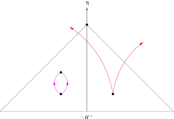
Figure 4: Short wavelength – $\lambda_{\rm phys}<H^{-1}$ – graviton pairs (violet) recombine while                      long wavelength – $\lambda_{\rm phys}>H^{-1}$ – ones (red) cannot.

More precisely, consider the mode functions $u_{dS}(t,k)$ of free gravitons:

$$u_{dS}(t,k)\;=\;\frac{1}{\sqrt{2k}}\left[\;{\it\Omega}_{dS}^{-1}+\frac{iH}{k}\;\right]e^{-ik\eta}\;\;.$$ (56)

It follows from (51) that the physical energy of the vacuum in mode ${\vec{k}}$ is:

$$E_{dS}(t,{\vec{k}})\;=\;\frac{1}{2}\,k\,e^{-Ht}\,+\,{H^{2}\,e^{Ht}\over 4k}\;\;.$$ (57)

The first term is just the – properly redshifted – minimum energy; the second term is the result of particle production. A typical mode begins at $t=0$ with the first term dominant. The second term becomes comparable at “horizon crossing” and dominates thereafter. This is the source of inflationary particle creation, and the onset of this enormous growth is what distinguishes infrared and ultraviolet modes. Horizon crossing of a mode occurs when its physical wave number equals the Hubble constant:

$${\it Horizon\;Crossing}\quad\Longrightarrow\quad k_{\rm phys}\,=\,k\;a_{dS}^{-1}(t)\,=\,H\;\;,$$ (58)

and provides the physical separation between infrared and ultraviolet modes:

$${\it Infrared}\quad \Longrightarrow \quad H<k<H\,e^{Ht}\;\;,$$ (59)

$${\it Ultraviolet}\quad \Longrightarrow \quad k>H\,e^{Ht}\;\;.$$ (60)

Furthermore, from (52) we can obtain the number of gravitons created for a particular mode:

$$N_{dS}(t,{\vec{k}})\;=\;\frac{1}{4}\left[\,1\,+\,\left(\frac{H\,e^{Ht}}{2k}\right)^{2}\,\right]\;\;,$$ (61)

and verify conditions (53-54):

$${\it Infrared}\quad \Longrightarrow \quad N_{\rm IR}^{dS}(t,{\vec{k}})\,\sim\,\left(\frac{H\,e^{Ht}}{2k}\right)^{2}\;\gg\;1\;\;,$$ (62)

$${\it Ultraviolet}\quad \Longrightarrow \quad N_{\rm UV}^{dS}(t,{\vec{k}})\,\sim\,0\;\;.$$ (63)

Finally, it is useful to record the infrared and ultraviolet limits of the mode functions (93):

$${\it Infrared}\quad \Longrightarrow \quad u_{\rm IR}^{dS}(t,k)\,\sim\,\frac{iH}{\sqrt{2k^{3}}}\;\;,$$ (64)

$${\it Ultraviolet}\quad \Longrightarrow \quad u_{\rm UV}^{dS}(t,k)\,\sim\,\frac{{\it\Omega}_{dS}^{-1}}{\sqrt{2k}}\;e^{-ik\eta}\;\;.$$ (65)

To get a sense of the density of infrared gravitons present per causal volume, we express the number of Hubble volumes in terms of the initial condition $H(0)=H$:

$$N_{H}(t)\;=\;\left[\;\frac{H(t)\;a(t)}{H}\;\right]^{3}\;\;.$$ (66)

For the inflationary geometry, we trivially get:

$$N^{dS}_{H}(t)\;=\;e^{3Ht}\;\;,$$ (67)

so that – within one Hubble volume – the number of any infrared gravitons at time $t$ is given by:

$$N_{\rm IR}^{dS}(t)\;=\;\frac{1}{N^{dS}_{H}(t)}\times\frac{1}{2\pi^{2}H^{3}}\int_{H}^{He^{Ht}}dk\;k^{2}\times N_{\rm IR}^{dS}(t,{\vec{k}})\;=\;\frac{1}{8\pi^{2}}\;\;.$$ (68)

The presence of about one infrared graviton in each Hubble volume implies that the initial vacuum choice and perturbation theory is an excellent approximation during the inflationary regime. Such a low density cannot by itself drive a significant infrared screening effect; the coherent superposition from all infrared gravitons does.

(iii) The Inflationary Rule
To make the connection of the physical picture with the quantum field theoretic results presented in Section 2, consider the first non-trivial contribution to the induced stress tensor in the graviton-like scalar model (33) described therein. Its leading part is:

$$T_{\mu\nu}^{\,\colon\varphi\colon}\ \sim\ -\ g_{\mu\nu}^{\,dS}\;\left\langle 0\left|\;\frac{1}{4!}\lambda\;\colon\varphi^{4}\colon\;\right|0\right\rangle\;\;.$$ (69)

The relevant diagram (see Figure 3) has been calculated [9] in conformal coordinates where the Feynman rules are particularly simple. For large observation times, the answer can be written in the following suggestive form:

$$T_{\mu\nu}^{\,\colon\varphi\colon}\,(\eta)\ \sim\;{\it\Omega}_{dS}^{2}\;\eta_{\mu\nu}\;\;\frac{\lambda^{2}H^{4}}{2^{9}\ 3^{2}\ \pi^{6}}\;\times\;\ln{\it\Omega}_{dS}\;\times\;\ln^{3}{\it\Omega}_{dS}\;\;.$$ (70)

In co-moving coordinates:

$$T_{\mu\nu}^{\,\colon\varphi\colon}\,(t)\ \sim\;g_{\mu\nu}^{\,dS}\;\;\frac{\lambda^{2}H^{4}}{2^{9}\ 3^{2}\ \pi^{6}}\;\times\;(Ht)\;\times\;(Ht)^{3}\;\;.$$ (71)

Expressions for the induced energy density and pressure follow immediately from (7):

$$\rho_{dS}^{\colon\varphi\colon}\,(t) = -\frac{\lambda^{2}H^{4}}{2^{9}\ 3^{2}\ \pi^{6}}\left[\;(Ht)^{4}\;+\;O(H^{3}t^{3})\;\right]+\;O(\lambda^{3})\;\;,$$ (72)

$$p_{dS}^{\colon\varphi\colon}\,(t) = \frac{\lambda^{2}H^{4}}{2^{9}\ 3^{2}\ \pi^{6}}\left[\;(Ht)^{4}\;+\;O(H^{3}t^{3})\;\right]+\;O(\lambda^{3})\;\;.$$ (73)

The observer has causal access to the volume of the past lightcone:

$$V_{\rm PLC}^{dS}(\eta)=\int_{-\frac{1}{H}}^{\eta}d\eta^{\prime}\,\,{\it\Omega}_{dS}^{\,4}(\eta^{\prime})\;\;\frac{4\pi}{3}\left(\eta-\eta^{\prime}\right)^{3}\;\;,$$ (74)

which for large observation times becomes:

$$V_{\rm PLC}^{dS}(\eta)\;\longrightarrow\;\frac{4\pi}{3}H^{-4}\;\ln{\it\Omega}_{dS}\ =\ \frac{4\pi}{3}H^{-4}\;\left(Ht\right)\;\;.$$ (75)

This is a purely geometrical quantity, independent of the particular dynamics of the theory. It controls the size over which particle production can affect a local observer and is responsible for the single $\ln{\it\Omega}_{dS}=Ht$ factor in (70-71) since the diagram contains a single interaction vertex integration.

The correlations are imprinted on the propagator:

$$i\Delta_{dS}(x;x^{\prime}) = \frac{H^{2}}{8\pi^{2}}\left\{\frac{2\eta\eta^{\prime}}{{\it\Delta}x^{2}-(|{\it\Delta}\eta|-i\epsilon)^{2}}-\ln\left[H^{2}\left({\it\Delta}x^{2}-(|{\it\Delta}\eta|-i\epsilon)^{2}\right)\right]\right\}\;\;,$$ (76)

$${\it\Delta}\eta\equiv\eta-\eta^{\prime}\quad\&\quad{\it\Delta}x\equiv\|{\vec{x}}-{\vec{x}}^{\,\prime}\|\;\;.$$

Particle production resides in the logarithmic term of the propagator; its absence reduces (76) to the flat space situation for which there is no such production. The propagator also carries the long-range field that emerges from the particles produced. In (70-71) the propagator is responsible for the factor $\ln^{3}{\it\Omega}_{dS}=(Ht)^{3}$ since the diagram represents an expectation value and, therefore, its leading part contains the cube of the real part of (76).

The induced stress tensor can be thought of as the combined result of a geometrical effect – the causal volume accessed by the observer – and a dynamical effect – the interaction stress among the particles produced:

$${\it Inflationary\;Induced\;Stress}\;\sim$$ (77)

$${\it``Causal\;Volume"}\;\times\;{\it``Interactions\;Among\;Particles\;Produced"}\;\;.$$

The effect is inherently non-local, as it should be. Otherwise, it could not screen $\Lambda$; it would be absorbable into a re-definition of $\Lambda$.

(iv) Deflation is Unavoidable
Deflation must occur because, as the inflationary expansion rate is reduced, the visible region of inflationary particle production continues to increase at an even faster pace and correlations remain basically the same. The screening effect grows stronger and makes the expansion rate slow even more. There simply is no barrier preventing the universe to enter a contracting phase. This behaviour of the screening mechanism is a generic gravitational instability. A familiar example is the instability of black holes emitting Hawking radiation: as they emit radiation their temperature increases and makes them emit even more.

We use Latin characters to distinguish deflationary quantities from their inflationary counterparts:

$${\rm a}(t)=\exp\left[\,{\rm b}(t)\,\right]=\Omega(\eta)\quad,\quad{\dot{\hskip 4.26773pt{\rm b}}}(t)<0\;\;.$$ (78)

The spacetime geometry (78) results in a completely unacceptable classical cosmology. The total energy density $\rho_{\rm T}$ and pressure $p_{\rm T}$ of any classically stable theory in a homogeneous and isotropic universe must obey the weak energy condition [17]:

$$\rho_{\rm T}+p_{\rm T}\;\geq\;0\;\;.$$ (79)

From the evolution equation:

$$-2{\ddot{\hskip 2.84544pt{\rm b}}}\;=\;8\pi G\left(\rho_{\rm T}+p_{\rm T}\right)\;\;,$$ (80)

this is equivalent to ${\ddot{\hskip 2.84544pt{\rm b}}}(t)\leq 0$. Thus, if deflation occurs at $t=t_{1}$, it will continue to occur thereafter:

$${\dot{\hskip 4.26773pt{\rm b}}}(t_{1})<0\quad\Longrightarrow\quad{\dot{\hskip 2.84544pt{\rm b}}}(t)<0\quad,\quad\forall\;t>t_{1}\;\;,$$ (81)

and the universe will suffer total collapse.

The above analysis is based entirely on classical gravity and can only be invalidated by quantum gravitational effects. We shall argue that such an effect is present and leads to a recovery from the deflationary regime. It is worthwhile mentioning at this stage that such a quantum violation of the weak energy condition leads to an equation of state which cannot be produced by any cosmology based on classical gravity:

$$\rho_{\rm T}+p_{\rm T}\;<\;0\quad\Longleftrightarrow\quad w<-1\;\;,$$ (82)

where $p_{\rm T}=w\rho_{\rm T}$. An equation of state with $w<-1$ is a quite unique and distinctive prediction with observational consequences.

(v) The Physical Picture as Deflation Commences
The maximally symmetric example of a contracting universe is the de Sitter geometry (11) with a reflected Hubble constant. Therefore, to retain our quantitative power, we idealize the geometry as perfect de Sitter inflation with Hubble constant $H$, followed by perfect de Sitter deflation with Hubble constant $-H$. The transition is assumed to occur at co-moving time $t=t_{1}$:

$$a_{dS}(t) = \exp\left[\,b_{dS}(t)\,\right]\;=\;e^{Ht}\quad,\quad\forall\;0<t<t_{1}\;\;,$$ (83)

$${\rm a}_{\rm dS}(t) = \exp\left[\,{\rm b}_{\rm dS}(t)\,\right]\;=\;e^{-H(t-2t_{1})}\quad,\quad\forall\;t_{1}<t<+\infty\;\;.$$ (84)

The equivalent statement in conformal coordinates is:

$${\it\Omega}_{dS}(\eta) = -\frac{1}{H\eta}\quad,\quad\forall\;-H^{-1}<\eta<\eta_{1}\;\;,$$ (85)

$$\Omega_{\rm dS}(\eta) = \frac{1}{H(\eta-2\eta_{1})}\quad,\quad\forall\;\eta_{1}<\eta<+\infty\;\;.$$ (86)

Since the number of inflationary e-foldings (25) is very large, the co-moving transition time satisfies:

$$N_{1}\gg 60\quad\Longrightarrow\quad t_{1}\gg H^{-1}\;\;,$$ (87)

or, in the conformal language:

$$N_{1}\gg 60\quad\Longrightarrow\quad\eta_{1}=-H^{-1}e^{-N_{1}}\;\rightarrow\;0^{-}\quad\sim\quad|\eta_{1}|\ll H^{-1}\;\;.$$ (88)

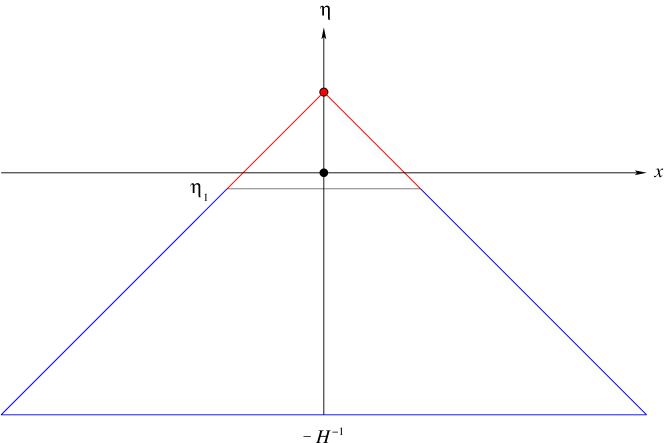
Figure 5: The past lightcone of an observer past the inflation (blue) to deflation                       (red) transition. The graph is not properly scaled.

The volume of the past lightcone of an observer at a post-transition time is (see Figure 5):

$${\rm V}_{\rm PLC}(\eta) = \int_{-\frac{1}{H}}^{\eta}d\eta^{\prime}\;{\it\Omega}^{4}(\eta^{\prime})\;\;\frac{4\pi}{3}\left(\eta-\eta^{\prime}\right)^{3}\;\;,$$ (89)

$$= \frac{4\pi}{3}H^{-4}\left\{\;\int_{-\frac{1}{H}}^{\eta_{1}}d\eta^{\prime}\;\frac{\left(\eta-\eta^{\prime}\right)^{3}}{\eta^{\prime 4}}+\int_{\eta_{1}}^{\eta}d\eta^{\prime}\;\frac{\left(\eta-\eta^{\prime}\right)^{3}}{\left(\eta^{\prime}-2\eta_{1}\right)^{4}}\;\right\}\;\;,\qquad$$ (90)

and for large observation times becomes:

$${\rm V}_{\rm PLC}(\eta)\;\longrightarrow\;\frac{8\pi}{9}H^{-4}\;\left(\frac{{\it\Omega}_{1}}{\Omega}\right)^{3}=\ \frac{8\pi}{9}H^{-4}\;e^{3H(t-t_{1})}\;\;.$$ (91)

The exponential increase with co-moving time of the past lightcone volume – as opposed to the linear increase (75) during inflation – has an obvious physical origin: as the universe deflates, causally disconnected regions come into contact again at a very rapid rate. Hence, some of the modes that left the horizon in the inflationary era, can causally interact again during the subsequent deflation.

More precisely, consider the inflationary mode expansion of the field operator for the massless, minimally coupled scalar appropriate to the Bunch-Davies vacuum:

$${\widetilde{\varphi}}(\eta,{\vec{k}}) = u(\eta,k)\;\alpha_{0}({\vec{k}})\;+\;u^{*}(\eta,k)\;\alpha_{0}^{\dagger}(-{\vec{k}})\;\;,$$ (92)

$$u(\eta,k) = \frac{1}{\sqrt{2k}}\left[\;{\it\Omega^{-1}}(\eta)+\frac{iH}{k}\;\right]e^{-ik\eta}\;\;.$$ (93)

We can retain this expansion by simply evolving the mode functions into the deflationary epoch. However, it is useful to expand the same field operator in the different basis appropriate to the Bunch-Davies vacuum for deflation:

$${\widetilde{\varphi}}(\eta,{\vec{k}}) = {\rm v}(\eta,k)\;\alpha_{1}({\vec{k}})\;+\;{\rm v}^{*}(\eta,k)\;\alpha_{1}^{\dagger}(-{\vec{k}})\;\;,$$ (94)

$${\rm v}(\eta,k) = \frac{1}{\sqrt{2k}}\left[\;\Omega^{-1}(\eta)-\frac{iH}{k}\;\right]e^{-ik\eta}\;\;.$$ (95)

The evolution of (93) after the transition:

$${\it Inflation}\;\longrightarrow\;{\it Deflation}\quad\Longrightarrow\quad u(\eta,k)\;\longrightarrow\;{\rm u}(\eta,k)\;\;,$$ (96)

is obtained by matching the mode functions and their first derivative at $\eta=\eta_{1}$:

$${\rm u}(\eta,k)=\left[\;1+\frac{iH{\it\Omega}_{1}}{k}\;\right]{\rm v}(\eta,k)\;+\;\left[\;\frac{iH{\it\Omega}_{1}}{k}\;e^{-2ik\eta_{1}}\;\right]{\rm v}^{*}(\eta,k)\;\;,$$ (97)

where ${\it\Omega}_{1}\equiv-(H\eta_{1})^{-1}$. Hence, the relation between the operators in the two regimes is:

$$\alpha_{1}(\vec{k})=\left[\;1+\frac{iH{\it\Omega}_{1}}{k}\;\right]\alpha_{0}(\vec{k})\;-\;\left[\;\frac{iH{\it\Omega}_{1}}{k}\;e^{-2ik\eta_{1}}\;\right]\alpha_{0}^{\dagger}(-{\vec{k}})\;\;.$$ (98)

The connection between the corresponding Bunch-Davies vacua:

$$\alpha_{0}\;\Big{|}\hskip 1.42271pt0\Big{\rangle}=0\quad\&\quad\alpha_{1}\;\Big{|}\hskip 1.42271pt1\Big{\rangle}=0\;\;,$$ (99)

is a direct implication of (98):

$$\Big{|}\hskip 1.42271pt1\Big{\rangle}\sim\;\exp{\left[\;\frac{e^{-2ik\eta_{1}}}{2\;(1+ik\eta_{1})}\;{\left(\alpha_{0}^{\dagger}\right)^{2}}\;\right]}\;\Big{|}\hskip 1.42271pt0\Big{\rangle}\;\;,$$ (100)

and clearly displays the vast number of particles with which the inflationary vacuum has been populated.

It is useful to decompose ${\rm u}(\eta,k)$ into two parts:

$${\rm u}(\eta,k)\;=\;{\rm v}(\eta,k)\,+\,{\rm U}(\eta,k)\;\;,$$ (101)

where (97) requires:

$${\rm U}(\eta,k)\;\equiv\;\frac{iH{\it\Omega}_{1}}{k}\;e^{-ik\eta_{1}}\left[\ e^{ik\eta_{1}}\;{\rm v}(\eta,k)+e^{-ik\eta_{1}}\;{\rm v}^{*}(\eta,k)\ \right]\;\;.$$ (102)

We can rewrite (102) as follows:

$${\rm U}(\eta,k)={\sqrt{\frac{2}{k}}}\;\frac{H}{k}\;\frac{{\it\Omega}_{1}}{\Omega}\;ie^{-ik\eta_{1}}\left\{{\cos\left[k(\eta-\eta_{1})\right]}\ -\ \frac{H\Omega}{k}\;{\sin\left[k(\eta-\eta_{1})\right]}\right\}$$ (103)

Due to the infinitesimal proximity of the transition conformal time $\eta_{1}$ to $0^{-}$, the oscillating argument in (103) can be excellently approximated:

$$k\;(\eta-\eta_{1})\;\sim\;k\;(\eta-2\eta_{1})\;=\;\frac{k}{H\Omega}\;\equiv\;{\rm x}\;\;,$$ (104)

so that:

$${\rm U}(\eta,k)\ \sim\ {\sqrt{\frac{2}{k}}}\;\frac{H}{k}\;\frac{{\it\Omega}_{1}}{\Omega}\;ie^{-ik\eta_{1}}\left(\cos{\rm x}\ -\ \frac{\sin{\rm x}}{{\rm x}}\right)\;\;.$$ (105)

The number of available gravitons of a particular mode is obtained by substituting (97) in (52):

$${\rm N}(t,{\vec{k}}) = \frac{1}{4}\left(1+2\,\frac{H^{2}{\it\Omega}_{1}^{2}}{k^{2}}\right)\left(1+\frac{H^{2}\,\Omega^{2}}{k^{2}}\right)$$ (106)

$$+\;\frac{1}{4}\;\frac{iH{\it\Omega}_{1}}{k}\left(1-\frac{iH{\it\Omega}_{1}}{k}\right)\left(1+\frac{iH\Omega}{k}\right)^{2}\;e^{2ik(\eta-\eta_{1})}$$

$$-\;\frac{1}{4}\;\frac{iH{\it\Omega}_{1}}{k}\left(1+\frac{iH{\it\Omega}_{1}}{k}\right)\left(1-\frac{iH\Omega}{k}\right)^{2}\;e^{-2ik(\eta-\eta_{1})}\;\;.$$

In a deflating geometry – unlike an inflating one – there is no horizon and, hence, no particle creation. From (101) and (106), which take into account that deflation followed an inflationary epoch, we can physically distinguish three kinds of modes. Keeping in mind that from the transition onwards ${\it\Omega}_{1}\gg\Omega$, we have:
$\ast$ Infrared modes, characterized by the smallest wave numbers and high occupancy,

$${\it Infrared}\quad \Longrightarrow \quad H<k<H\,\Omega\;\;,$$ (107)

$$\Longrightarrow \quad{\rm u}_{\rm IR}(t,k)\;\sim\;-\frac{iH}{\sqrt{2k^{3}}}\;\;,$$ (108)

$$\Longrightarrow \quad{\rm N}_{\rm IR}(t,{\vec{k}})\,\sim\,\frac{H^{2}\,{\it\Omega}_{1}^{2}}{2k^{2}}\;\gg\;1\;\;.$$ (109)

As (109) indicates, infrared modes are not produced after $t_{1}$; they were created during inflation when they could not recombine and they continue to exist thereafter. A typical infrared mode (107) satisfies ${\rm x}\ll 1$ and, therefore, $\cos{\rm x}$ almost cancels against ${\rm x}^{-1}\sin{\rm x}$ in (105) to leave a negligible contribution to ${\rm U}(\eta,k)$. The mode functions (108) come solely from the ${\rm v}(\eta,k)$ part of (101).
$\ast$ Ultraviolet modes, characterized by the largest wave numbers and low occupancy,

$${\it Ultraviolet}\quad \Longrightarrow \quad k>H{\it\Omega}_{1}\;\;,$$ (110)

$$\Longrightarrow \quad{\rm u}_{\rm UV}(t,k)\;\sim\;\frac{\Omega^{-1}}{\sqrt{2k}}\;e^{-ik\eta}\;\;,$$ (111)

$$\Longrightarrow \quad{\rm N}_{\rm UV}(t,{\vec{k}})\,\sim\,0\;\;.$$ (112)

They are virtual throughout the entire evolution. Because a typical ultraviolet mode (110) obeys ${\rm x}\gg{\Omega}^{-1}{\it\Omega}_{1}\gg 1$ , only the $\cos{\rm x}$ term survives in (103). Nonetheless, it is multiplied by the ultraviolet factor $k^{-\frac{3}{2}}$ so that the corresponding mode functions (111) reside exclusively in the ${\rm v}(\eta,k)$ part of (101).
$\ast$ Thermal modes, characterized by the remaining wave numbers and – in the typical case – high occupancy,

$${\it Thermal}\quad \Longrightarrow \quad H\,\Omega<k<H{\it\Omega}_{1}\;\;,$$ (113)

$$\Longrightarrow \quad{\rm u}_{\rm TH}(t,k)\,\sim\,{\sqrt{\frac{2}{k}}}\;\frac{H}{k}\;\frac{{\it\Omega}_{1}}{\Omega}\;\cos\left(\frac{k}{H\Omega}\right)\;\;,$$ (114)

$$\Longrightarrow \quad{\rm N}_{\rm TH}(t,{\vec{k}})\,\sim\,\frac{H^{2}\,{\it\Omega}_{1}^{2}}{k^{2}}\;\cos^{2}\left(\frac{k}{H\Omega}\right)\;\gg\;1\;\;.\qquad$$ (115)

These are, by virtue of their large occupation number, “infrared” modes during deflation. However, their wavelength allows them to potentially recombine after the transition at $t_{1}$. From (115), it is apparent that perfect annihilation occurs only when:

$$k_{\rm phys}\;=\;k\,\Omega^{-1}\,\sim\;\pi H\left(\ell+\frac{1}{2}\,\right)\quad,\quad\forall\,\ell\in{\cal N}_{0}\;\;.$$ (116)

For a typical thermal mode (113), where $1\ll{\rm x}\ll{\Omega}^{-1}{\it\Omega}_{1}$ , only the $\cos{\rm x}$ term survives in (103) and it is multiplied by ${\Omega}^{-1}{\it\Omega}_{1}\gg 1$. Therefore, it is the thermal modes which contribute to ${\rm U}(\eta,k)$ and that contribution is big. It is important to note that right after the transition at $t_{1}$, ${\rm u}_{\rm TH}(\eta,k)$ behaves like ${\rm u}_{\rm IR}(\eta,k)$, that is, like a constant. But as soon as the contracting $\Omega$ has shrunk to the point that the $\Omega^{-1}$ term overwhelms the $iHk^{-1}$ term, ${\rm u}_{\rm TH}(\eta,k)$ starts to blueshift like $\Omega^{-1}$ – in contradistinction to ${\rm u}_{\rm IR}(\eta,k)$ which always stays constant. The “crossover” when the constant thermal mode functions behaviour becomes a growth is given by $k\sim H\Omega$.

Finally, a deflationary observer can measure the density of any thermal gravitons per invariant 3-volume:

$${\rm\rho}_{\rm TH}(t)=\frac{H^{3}}{{\rm a}^{3}(t)}\times H^{-3}\int_{H\Omega}^{H{\it{\Omega}_{1}}}dk\;k^{2}\times{\rm N}_{\rm TH}(t,{\vec{k}})\;\sim\;H^{3}\;e^{H(t-t_{1})}\;\;,$$ (117)

and conclude that it increases exponentially with co-moving time.

(vi) Perturbation Theory is Revised
Perturbative computations in the presence of the state (15) are no longer appropriate. The density of thermal modes grows exponentially due to the contracting 3-volume. A part of the quantum field is effectively behaving like a classical field. Thus, we can absorb it into the background and use the classical field equations – which can be solved – to follow its non-perturbative evolution.

More precisely, the full quantum field (39) is decomposed into two parts:

$$\varphi(\eta,{\vec{x}})=\phi(\eta,{\vec{x}})\;+\;\Phi(\eta,{\vec{x}})\;\;.$$ (118)

The quantum field $\phi(\eta,{\vec{x}})$ is the mode expansion corresponding to a state which is in Bunch-Davies vacuum at the start of deflation:

$$\phi(\eta,{\vec{x}})=\int\frac{d^{3}k}{(2\pi)^{3}}\;e^{i{\vec{k}}\cdot{\vec{x}}}\;\left\{\;{\rm v}(\eta,k)\;\alpha_{0}({\vec{k}})\;+\;{\rm v}^{*}(\eta,k)\;\alpha_{0}^{\dagger}(-{\vec{k}})\;\right\}\;\;,$$ (119)

while the field $\Phi(\eta,{\vec{x}})$ expresses the enormous occupancies of the thermal and infrared modes for the actual state:

$$\Phi(\eta,{\vec{x}})=\int\frac{d^{3}k}{(2\pi)^{3}}\;e^{i{\vec{k}}\cdot{\vec{x}}}\;\left\{\;{\rm U}(\eta,k)\;\alpha_{0}({\vec{k}})\;+\;{\rm U}^{*}(\eta,k)\;\alpha_{0}^{\dagger}(-{\vec{k}})\;\right\}\;\;.$$ (120)

The latter commutes with its time derivative:

$$\left[\;{\widetilde{\Phi}}(\eta,{\vec{k}})\;,\,{\widetilde{\Phi}}^{\prime}(\eta,{\vec{k}}^{\prime})\;\right]\;=\;0\;\;,$$ (121)

so that its quantum fluctuations are essentially frozen. Strictly speaking, it is still a quantum field since it has an expansion (120) in terms of creation and annihilation operators. However, by giving random assignments to $\alpha_{0}$ and $\alpha_{0}^{\dagger}$ it can be treated, thereafter, as a classical field. The appearance of a continuously increasing number of thermal modes, makes perturbative calculations in the presence of the state (15) invalid. Accordingly, the field $\Phi$ – which describes the “hot dense soup” of thermal modes – should be considered as a classical background with the understanding that $\alpha_{0}$ and $\alpha_{0}^{\dagger}$ have been assigned random values. Hence, the “hot dense soup” of particles formed is taken into account by being treated as a classical background. It is around this stochastic background that perturbation theory must be developed. This revised perturbation theory will remain valid after $\Phi$ becomes strong enough for its self-interactions to become relevant.

The field $\Phi$ defined by (120) and (114) can be reduced as follows:

$$\Phi(\eta)\;\sim\;\int_{H\Omega}^{H{\it\Omega}_{1}}\frac{d^{3}k}{(2\pi)^{3}}\;{\sqrt{\frac{2}{k}}}\;\frac{H}{k}\;\frac{{\it\Omega}_{1}}{\Omega}\;{\cos\left(\frac{k}{H\Omega}\right)}\;i\left[\;\alpha_{0}({\vec{k}})\;-\;\alpha_{0}^{\dagger}(-{\vec{k}})\;\right]\;\;,$$ (122)

where we have exploited the negligible spatial variation of all thermal modes except those with $k\sim H{\it\Omega}_{1}$.

(vii) Evaluation of the Stochastic Background
Since the initial state (15) is free, the associated operators $\alpha_{0}$ and $\alpha_{0}^{\dagger}$ are stochastically realized as independent complex Gaussian random variables on the manifold $T^{3}$ with coordinate range (13). The commutation relations (47) imply that the independent stochastic variables $\alpha_{0}$ and $\alpha_{0}^{*}$ have standard deviation equal to $H^{-3}$. It is convenient to absorb the dimensions:

$$A_{\vec{n}}\;\equiv\;H^{\frac{3}{2}}\;\alpha_{0}(\vec{n})\quad\&\quad A^{*}_{\vec{n}}\;\equiv\;H^{\frac{3}{2}}\;\alpha_{0}^{*}(\vec{n})\;\;,$$ (123)

so that the standard deviation of the rescaled variables is one:

$$\sigma^{2}_{A}(\eta)\;=\;\sigma^{2}_{A^{*}}(\eta)\;=\;1\;\;.$$ (124)

In terms of the variables (123), the stochastic background (122) equals:

$$\Phi(\eta)\;\sim\;\frac{iH}{2\pi^{\frac{3}{2}}}\;\frac{{\it\Omega}_{1}}{\Omega}\;\sum_{\vec{n}}\;n^{-\frac{3}{2}}\;{\cos\left(\frac{2\pi}{\Omega}n\right)}\;\left[\;A_{\vec{n}}-A^{*}_{-{\vec{n}}}\;\right]\;\;,$$ (125)

where the summation range is $(2\pi)^{-1}\Omega<n<(2\pi)^{-1}{\it\Omega}_{1}$ . Its standard deviation is given by:

$$\sigma^{2}_{\Phi}(\eta)\;\sim\;\frac{H^{2}}{4\pi^{3}}\;\left(\frac{{\it\Omega}_{1}}{\Omega}\right)^{2}\;\sum_{\vec{n}}\;n^{-3}\;{\cos^{2}\left(\frac{2\pi}{\Omega}n\right)}\;\;,$$ (126)

and the sum present in (126) can be evaluated:

$$\sum_{\vec{n}}\;n^{-3}\;{\cos^{2}\left(\frac{2\pi}{\Omega}n\right)} \sim 4\pi\int_{\frac{\Omega}{2\pi}}^{\frac{{\it\Omega}_{1}}{2\pi}}\;\frac{dy}{y}\;\frac{1}{2}\left[\;1+{\cos\left(\frac{4\pi}{\Omega}y\right)}\;\right]\;\;,$$ (127)

$$= 2\pi\;\ln{\left(\frac{{\it\Omega}_{1}}{\Omega}\right)}\;+\;{\it O}(1)\;\;.$$ (128)

Therefore, a good measure of the stochastic background $\Phi$ is:

$$\Phi(\eta)\;\sim\;\sqrt{\sigma^{2}_{\Phi}(\eta)}\;\sim\;\frac{H}{{\sqrt{2}}\,\pi}\;\left(\frac{{\it\Omega}_{1}}{\Omega}\right)\;\sqrt{\ln{\left(\frac{{\it\Omega}_{1}}{\Omega}\right)}}\;\;.$$ (129)

4 The Deflationary Regime

(i) The Physical Picture During Deflation
Throughout the inflationary era there was production of infrared gravitons with a density of about one per Hubble volume. As deflation proceeds, the volume contracts and thermal modes appear; the first to do so have wave number $k=H{\it\Omega}_{1}$. Thereafter, modes with lower wave numbers follow and the density of any such thermal gravitons per invariant 3-volume increases dramatically (117).

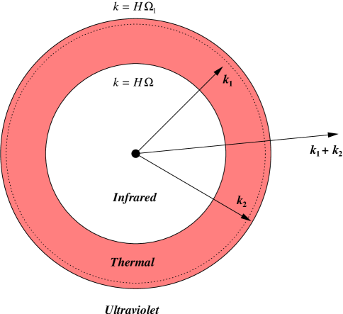
Figure 6: The 3-sphere of co-moving $k$ modes during deflation. The graph is not                       properly scaled.

Infrared modes produced during inflation can now scatter in the dense bath of thermal modes. Since there are more modes as $k$ increases, and, since the thermal modes with the highest $k$ appear first, it is more likely for an infrared mode to scatter with high $k$ thermal modes. This scattering process can increase the wave number $k<H\Omega$ of the infrared mode and turn it into a wave number $k>H{\it\Omega}_{1}$ of an ultraviolet mode (see Figure 6). Hence, the population of infrared modes or, equivalently, the amplitude of their mode functions decreases. It is this decrease that is responsible for terminating the growth of the strong infrared effect right after the transition from inflation to deflation occurs. Moreover, as we shall see, it ensures that deflation must end.

(ii) The Infrared Decay Rate
The calculation of the decay rate shall be done in the context of the graviton-like scalar model of Section 2. The dominant process, to lowest order in perturbation theory, is shown in Figure 7. As long as there is a diffuse small density of infrared modes – the production of which is the source of the effect – perturbation theory gives reliable results.

Figure 7: The dominant scattering process during deflation.

In terms of the differential transition probability $dP$, the transition rate $\Gamma$ per unit conformal time is given by:

$$\Gamma(\eta,k)=\frac{d}{d\eta}\,\int dP\left({\vec{k}}\,\rightarrow\,{\vec{k}}_{1}\,,{\vec{k}}_{2}\,,{\vec{k}}_{3}\right)\;\;,$$ (130)

where $\eta$ is the observation conformal time. The differential transition probability is obtained from the transition amplitude ${\it m}$ for the process:

$$dP\left({\vec{k}}\,\rightarrow\,{\vec{k}}_{1}\,,{\vec{k}}_{2}\,,{\vec{k}}_{3}\right) = \|\,\mbox{\Large${\it m}$}\left({\vec{k}}\,\rightarrow\,{\vec{k}}_{1}\,,{\vec{k}}_{2}\,,{\vec{k}}_{3}\right)\|^{2}\;\times$$

$$\frac{d^{3}{\vec{k}}_{1}}{(2\pi)^{3}}\;\frac{d^{3}{\vec{k}}_{2}}{(2\pi)^{3}}\;\frac{d^{3}{\vec{k}}_{3}}{(2\pi)^{3}}\;(2\pi)^{3}\,\delta^{3}\left({\vec{k}}-{\vec{k}}_{1}-{\vec{k}}_{2}-{\vec{k}}_{3}\right)\;\;,$$

where:

$$i\mbox{\Large${\it m}$}\left({\vec{k}}\,\rightarrow\,{\vec{k}}_{1}\,,{\vec{k}}_{2}\,,{\vec{k}}_{3}\right)\;(2\pi)^{3}\,\delta^{3}\left({\vec{k}}-{\vec{k}}_{1}-{\vec{k}}_{2}-{\vec{k}}_{3}\right)\equiv$$ (132)

$$\hskip 150.79968pt\Big{\langle}0\ \Big{|}\;\alpha_{0}({\vec{k}}_{1})\;\alpha_{0}({\vec{k}}_{2})\;\alpha_{0}({\vec{k}}_{3})\;\times$$

$$\quad{\bf T}\left\{\;\exp\left[\,-i\frac{\lambda}{4!}\,\int_{\eta_{1}}^{\eta}d\eta^{\prime}\;\Omega^{4}(\eta^{\prime})\;\int d^{3}x^{\prime}\;\varphi^{4}(\eta^{\prime},{\vec{x}}^{\;\prime})\,\right]\;\right\}\;\alpha_{0}^{\dagger}({\vec{k}})\;\Big{|}\ 0\Big{\rangle}\;\;.$$

Using the expansion (118-120) of the field and the canonical commutation relations (47), the transition amplitude takes the following form in terms of the mode functions (101):

$$i\mbox{\Large${\it m}$}\left({\vec{k}}\,\rightarrow\,{\vec{k}}_{1}\,,{\vec{k}}_{2}\,,{\vec{k}}_{3}\right)=$$ (133)

$$\quad-i\lambda\int_{\eta_{1}}^{\eta}d\eta^{\prime}\;\Omega^{4}(\eta^{\prime})\;\;{\rm u}^{*}(\eta^{\prime},k_{1})\;{\rm u}^{*}(\eta^{\prime},k_{2})\;{\rm u}^{*}(\eta^{\prime},k_{3})\;{\rm u}(\eta^{\prime},k)\;+\;O(\lambda^{2})\;\;.$$

The form of the mode functions appropriate for the infrared wave number $k$, the ultraviolet wave number $k_{3}$ and the thermal wave numbers $k_{1,2}$, was obtained in (108-114):

$${\rm u}(\eta,k) = {\rm u}_{\rm IR}(\eta,k)\;\sim\;-\frac{iH}{\sqrt{2k^{3}}}\;\;,$$ (134)

$${\rm u}(\eta,k_{3}) = {\rm u}_{\rm UV}(\eta,k_{3})\;\sim\;\frac{\Omega^{-1}}{\sqrt{2k_{3}}}\;e^{-ik_{3}\eta}\;\;,$$ (135)

$${\rm u}(\eta,\,k_{1,2}) = {\rm u}_{\rm TH}(\eta,\,k_{1,2})\;\sim\;\sqrt{\frac{2}{k_{1,2}}}\;\frac{iH}{k_{1,2}}\;\frac{{\it\Omega}_{1}}{\Omega}\;{\cos\left(\frac{k_{1,2}}{H\Omega}\right)}\;\;.$$ (136)

The observation time is taken to be well in-between the onset of inflation at $-H^{-1}$ and the transition time from inflation to deflation at $\eta_{1}$:

$$|\eta_{1}|\ll\eta\ll H^{-1}\;\;.$$ (137)

Typical wave numbers associated with the modes of the process satisfy:

$$H\ll k\ll H\Omega\ll k_{1,2}\ll H{\it\Omega}_{1}\ll k_{3}\;\;.$$ (138)

By substituting (134-136) in (133), the transition rate becomes:

$$\Gamma(\eta,k)\;\sim\;\lambda^{2}\,H^{6}\,{\it\Omega}_{1}^{4}\;\frac{\Omega}{k^{3}}\;\int_{\eta_{1}}^{\eta}d\eta^{\prime}\;\Omega(\eta^{\prime})\;\int\frac{d^{3}{\vec{k}}_{1}}{(2\pi)^{3}}\;\frac{\cos(k_{1}\eta)\,\cos(k_{1}\eta^{\prime})}{k_{1}^{3}}\;\times$$

$$\int\frac{d^{3}{\vec{k}}_{2}}{(2\pi)^{3}}\;\frac{\cos(k_{2}\eta)\,\cos(k_{2}\eta^{\prime})}{k_{2}^{3}}\;\;\frac{\cos\left[\,\|{\vec{k}}_{1}+{\vec{k}}_{2}\|\,(\eta-\eta^{\prime})\,\right]}{\|{\vec{k}}_{1}+{\vec{k}}_{2}\|}\;\;,\quad$$ (139)

where we used:

$${\vec{k}_{3}}={\vec{k}}-{\vec{k}_{1}}-{\vec{k}_{2}}\;\sim\;-\left({\vec{k}_{1}}+{\vec{k}_{2}}\right)\;\;.$$ (140)

Performing the angular integrations and noting that oscillatory destructive interference is avoided only when $k_{1,2}\ \Delta\eta\leq 1$, gives:

$$\Gamma(\eta,k)\;\sim\;\frac{\lambda^{2}\,H^{6}\,{\it\Omega}_{1}^{4}}{8\pi^{4}}\;\frac{\Omega}{k^{3}}\;\int_{t_{1}}^{t}dt^{\prime}\;\int_{H\Omega}^{H{\it\Omega}_{1}}\frac{dk_{1}}{k_{1}}\;\cos(k_{1}\,\Delta\eta)\;\times$$

$$\int_{H\Omega}^{H{\it\Omega}_{1}}\frac{dk_{2}}{k_{2}}\,\cos(k_{2}\,\Delta\eta)\;\frac{\cos(k_{1}\,\Delta\eta)\;\sin(k_{2}\,\Delta\eta)}{k_{1}\,k_{2}\,\Delta\eta}\;\;.$$ (141)

The final answer is:

$$\Gamma(\eta,k)\;\sim\;\frac{\lambda^{2}\;H^{4}\;{\it\Omega}_{1}^{4}}{24\pi^{4}\;k^{3}}\;\;.$$ (142)

It is elementary to recover the transition rate in co-moving time:

$$\Gamma(t,k)\;=\;\Omega^{-1}\;\Gamma(\eta,k)\;\;,$$ (143)

and the decay rate $\tau$:

$$\frac{1}{\mbox{\Large$\tau$}}(t,k)\;=\;\frac{\Gamma(t,k)}{N_{\rm IR}({\vec{k}}\,;t)}\;\;.$$ (144)

Using (143) and (53), we obtain:

$$\frac{1}{\mbox{\Large$\tau$}}(t,k)\;\sim\;\frac{\lambda^{2}\,H^{2}}{6\pi^{4}}\;\frac{{\it\Omega}_{1}}{k}\;\left(\frac{{\it\Omega}_{1}}{\Omega}\right)^{3}\;=\;\frac{\lambda^{2}\,H^{2}}{6\pi^{4}}\;\frac{e^{Ht_{1}}}{k}\;e^{3H(t-t_{1})}\;\;,$$ (145)

and it becomes apparent that the process becomes very strong very quickly. A way to understand this comes from considering the volume of the co-moving modes sphere (see Figure 6). Since the number of modes of wave number $k$ grows dramatically with increasing $k$, almost all the volume of the sphere is concentrated close to the surface at $k=H{\it\Omega}_{1}$:

$${\rm V_{skin}}\ =\ \frac{4}{3}\pi\left(H{\it\Omega}_{1}\right)^{3}\left[\ 1-e^{-H{\it\Delta}t}\ \right]\;\sim\;\frac{4}{3}\pi\left(H{\it\Omega}_{1}\right)^{3}\ =\ {\rm V_{sphere}}\;\;.$$ (146)

(iii) The Induced Stress
During inflation, the source of the induced stress tensor was the production of infrared particles. The objective is to determine the evolution of the induced stress tensor after the transition to deflation. As it was just shown, in the deflationary regime there is a strong depletion of the infrared particles due to the presence of a thermal particle bath with which they can scatter and become ultraviolet. Accordingly, the mode functions during deflation must be degraded to account for this depletion.

This is properly achieved by solving for the propagator in the presence of the stochastic background (129). In this case, there are no more plane wave momentum states. Nonetheless, a reasonable approximation is obtained by noting that the dominant effect comes from coherent interactions between infrared modes and is diminished upon their depletion. Therefore, we use plane wave states which then scatter with the background and disappear from the population of infrared modes. Each mode function is effectively degraded by the exponential of the integral of minus the decay rate:

$${\bar{\rm u}}(t,k)\;\equiv\;\exp\left[-\frac{1}{2}\int_{t_{1}}^{t}dt^{\prime}\;\frac{1}{\mbox{\Large$\tau$}}(t^{\prime},k)\,\right]\;{\rm u}(t,k)\;\;.$$ (147)

The degradation factor can be estimated using (145):

$$\exp\left[-\frac{1}{2}\int_{t_{1}}^{t}dt^{\prime}\;\frac{1}{\mbox{\Large$\tau$}}(t^{\prime},k)\,\right]\;\sim\;-\frac{\lambda^{2}\,H}{2^{2}\,3^{2}\,\pi^{4}}\;\frac{e^{Ht_{1}}}{k}\;e^{3H(t-t_{1})}\;\;.$$ (148)

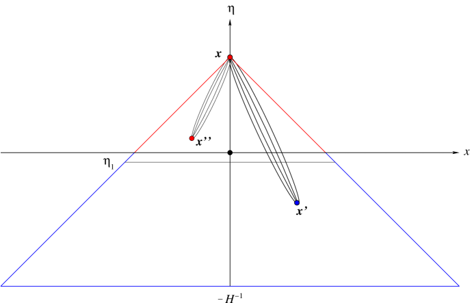
Figure 8: The dominant diagrammatic contribution to the induced ${\rm T}_{\mu\nu}^{\lambda^{2}}$ during                        deflation. The graph is not properly scaled.

Consider the first non-trivial contribution to the induced stress tensor. Its leading part:

$${\bar{\rm T}}_{\mu\nu}^{\,\colon\varphi\colon}\ \sim\ -g_{\mu\nu}\;\left\langle 0\left|\;\frac{1}{4!}\lambda\;\colon\varphi^{4}\colon\;\right|0\right\rangle\;\;,$$ (149)

has the same topology it did during inflation (see Figure 8). One of the two vertices is at the observation event at $x=(\eta,{\vec{0}})$. The other can be anywhere within the past lightcone of the observer and there are two possibilities. In the first, the vertex lies in the deflationary part – for instance, at $x^{\prime\prime}$ – and the mode functions both at $x$ and $x^{\prime\prime}$ must be degraded. But when the vertex is situated in the inflationary region – for instance, at $x^{\prime}$ – only the mode functions at $x$ must be degraded. Hence, it is the latter case that dominates and we shall concentrate on the corresponding diagram.

The exact calculation of the diagram using the degraded mode functions ${\bar{\rm u}}(t,k)$ at $x$, may not be feasible. A prohibitive fact is the presence of $k$ dependence in (148). It is apparent from (148), that the thermal screening effect caused by the presence of the degrading factor gets stronger with decreasing $k$. At the same time, the largest contribution to the induced stress tensor comes from infrared modes whose wave number is close to $k\sim H\Omega$. Thus, calculability can be restored by evaluating (148) at the wave number with the maximum impact: $k=H\Omega$. Such a procedure underestimates the thermal screening for $k<H\Omega$ and overestimates it for $k>H\Omega$. Nonetheless, these two deviations – being opposite in sign – can balance against each other. In this approximation, the desired answer is obtained from the one using ${\rm u}(t,k)$ by simple multiplication with an appropriate overall degrading factor:

$${\bar{\rm T}}_{\mu\nu}^{\,\colon\varphi\colon}\;\sim\;{\rm T}_{\mu\nu}^{\,\colon\varphi\colon}\;\exp\left[-2\int_{t_{1}}^{t}dt^{\prime}\;\frac{1}{\mbox{\Large$\tau$}}(t^{\prime},k)\,\right]_{k=H\Omega}\;\;.$$ (150)

The factor of 2 in the exponent of the degrading factor in (150) reflects the four mode functions present at $x$. From (148), it trivially follows that:

$$\exp\left[-2\int_{t_{1}}^{t}dt^{\prime}\;\frac{1}{\mbox{\Large$\tau$}}(t^{\prime},k)\,\right]_{k=H\Omega}\;\sim\;-\frac{\lambda^{2}}{9\,\pi^{4}}\;e^{4H(t-t_{1})}\;=\;-\frac{\lambda^{2}}{9\,\pi^{4}}\left(\frac{{\it\Omega_{1}}}{\Omega}\right)^{4}\;\;.$$ (151)

A straightforward application of the Schwinger-Keldysh rules to the dominant diagram of Figure 8, results in the following expression for the expectation value the diagram represents:

$${\rm T}_{\mu\nu}^{\,\colon\varphi\colon}\,(x)\;=\;\Omega^{2}\eta_{\mu\nu}\;\;\frac{i\lambda^{2}}{4!}\;\int d^{4}x^{\prime}\;{\it\Omega}^{4}(x^{\prime})\;\times$$

$$\hskip 85.35826pt\left\{\;\left[\;i\Delta_{++}(x;x^{\prime})\,\right]^{4}-\,\left[\;i\Delta_{+-}(x;x^{\prime})\,\right]^{4}\;\right\}\;\;.$$ (152)

Due to their correlated interactions, infrared modes comprise the ultimate source for the generation of a strong induced stress tensor. Under evolution into the deflationary regime, the mode functions of the still infrared modes remain unaltered from their inflationary form except for the sign change due to the Hubble parameter reflection. Therefore, it is again the logarithmic term in the propagator (76) that carries the leading effect:

$$i\Delta_{++}(x;x^{\prime})\;\sim\;-\frac{H^{2}}{8\pi^{2}}\;\ln\left[H^{2}\left({\it\Delta}x^{2}-({\it\Delta}\eta-i\epsilon)^{2}\right)\right]\;\;,$$ (153)

$$i\Delta_{+-}(x;x^{\prime})\;\sim\;-\frac{H^{2}}{8\pi^{2}}\;\ln\left[H^{2}\left({\it\Delta}x^{2}-({\it\Delta}\eta+i\epsilon)^{2}\right)\right]\;\;,$$ (154)

by providing, eventually, the maximum number of $\ln\Omega$ factors.

Decomposing into real and imaginary parts provides the leading contribution from the propagator combination appearing in (152):

$$\left[\;i\Delta_{++}(x;x^{\prime})\,\right]^{4}-\,\left[\;i\Delta_{+-}(x;x^{\prime})\,\right]^{4}\;\sim\;$$

$$\sim\;\frac{H^{8}}{2^{12}\,\pi^{8}}\;\Big{\{}\;\ln\left[H^{2}\left({\it\Delta}\eta^{2}-{\it\Delta}x^{2}\right)+i\pi\right]^{4}-\ln\left[H^{2}\left({\it\Delta}\eta^{2}-{\it\Delta}x^{2}\right)-i\pi\right]^{4}\Big{\}}$$

$$\sim\;\frac{H^{8}}{2^{12}\,\pi^{8}}\;8\pi i\,\ln^{3}\left[H^{2}\left({\it\Delta}\eta^{2}-{\it\Delta}x^{2}\right)\right]\;\;.\qquad$$ (155)

Using (155) and performing the angular integrations present in (152) gives:

$${\rm T}_{\mu\nu}^{\,\colon\varphi\colon}\,(\eta)\;\sim\;-\Omega^{2}\eta_{\mu\nu}\;\;\frac{\lambda^{2}\,H^{8}}{2^{10}\,3\,\pi^{6}}\;\int_{-\frac{1}{H}}^{\eta_{1}}d\eta^{\prime}\;{\it\Omega}^{4}(\eta^{\prime})\;\times$$

$$\hskip 93.89418pt{\it\Delta}\eta^{3}\int_{0}^{1}dy\;y^{2}\;\ln^{3}\left[H^{2}{\it\Delta}\eta^{2}\left(1-y^{2}\right)\right]\;\;,$$ (156)

where we have rescaled the radial variable $r\in\left[\,0\,,\,{\it\Delta}\eta\,\right]$ thusly:

$$r\equiv({\it\Delta}\eta)\;y\quad,\quad y\in\left[\,0\,,\,1\,\right]\;\;.$$ (157)

To leading order, the $y$ integration is:

$$\int_{0}^{1}dy\;y^{2}\;\ln^{3}\left[H^{2}{\it\Delta\eta}^{2}\left(1-y^{2}\right)\right] \sim 2^{3}\;\ln^{3}\left(H{\it\Delta\eta}\right)\int_{0}^{1}dy\;y^{2}$$ (158)

$$= \frac{2^{3}}{3}\;\ln^{3}\left(H{\it\Delta\eta}\right)\;\;,$$

so that we get:

$${\rm T}_{\mu\nu}^{\,\colon\varphi\colon}\,(\eta)\;\sim\;-\Omega^{2}\eta_{\mu\nu}\;\;\frac{\lambda^{2}\,H^{4}}{2^{7}\,3^{2}\,\pi^{6}}\;\int_{-\frac{1}{H}}^{\eta_{1}}\;\frac{d\eta^{\prime}}{\eta^{\prime\,4}}\;\Delta\eta^{3}\;\ln^{3}\left(H{\it\Delta\eta}\right)\;\;.$$ (159)

Because of (137) and the domination of the conformal time integration from the region close to its upper limit $\eta^{\prime}\sim\eta_{1}$, we have:

$$\int_{-\frac{1}{H}}^{\eta_{1}}\;\frac{d\eta^{\prime}}{\eta^{\prime\,4}}\;{\it\Delta}\eta^{3}\;\ln^{3}\left(H{\it\Delta}\eta\right) \sim \eta^{3}\;\ln^{3}(H\eta)\;\int_{-\frac{1}{H}}^{\eta_{1}}\;\frac{d\eta^{\prime}}{\eta^{\prime\,4}}$$ (160)

$$= -\frac{1}{3}\left(\frac{\eta}{\eta_{1}}\right)^{3}\;\ln^{3}(H\eta)\;\;.$$

Consequently:

$${\rm T}_{\mu\nu}^{\,\colon\varphi\colon}\,(\eta)\;\sim\;\Omega^{2}\eta_{\mu\nu}\;\;\frac{\lambda^{2}\,H^{4}}{2^{7}\,3^{3}\,\pi^{6}}\;\left(\frac{{\it\Omega}_{1}}{\Omega}\right)^{3}\;\ln^{3}\Omega\;\;.$$ (161)

The physically relevant induced stress tensor during deflation is obtained by substituting (161) and (151) in (150):

$${\bar{\rm T}}_{\mu\nu}^{\,\colon\varphi\colon}\,(\eta)\;\sim\;g_{\mu\nu}\;\;\frac{\lambda^{2}\,H^{4}}{2^{7}\,3^{3}\,\pi^{6}}\;\times\;\left(\frac{{\it\Omega}_{1}}{\Omega}\right)^{3}\;\times\;\ln^{3}\Omega\;\times\;e^{-\frac{\lambda^{2}}{9\,\pi^{4}}\;\left(\frac{{\it\Omega}_{1}}{\Omega}\right)^{4}}\;\;,$$ (162)

or, in co-moving coordinates:

$${\bar{\rm T}}_{\mu\nu}^{\,\colon\varphi\colon}\,(t)\;\sim\;g_{\mu\nu}\;\;\frac{\lambda^{2}\,H^{4}}{2^{7}\,3^{3}\,\pi^{6}}\;\times\;e^{3H(t-t_{1})}\;\times\;(Ht_{1})^{3}\;\times\;e^{-\frac{\lambda^{2}}{9\,\pi^{4}}\;e^{4H(t-t_{1})}}\;\;.$$ (163)

The induced energy density ${\varrho}$ and pressure ${\rm p}$ present in (163) follow directly from (7):

$${\varrho}^{\colon\varphi\colon}\,(t) \sim -\ \frac{\lambda^{2}\,H^{4}}{2^{7}\,3^{3}\,\pi^{6}}\;\;(Ht_{1})^{3}\;\;e^{3H(t-t_{1})}\;\;e^{-\frac{\lambda^{2}}{9\,\pi^{4}}\;e^{4H(t-t_{1})}}\;\;,$$ (164)

$${\rm p}^{\colon\varphi\colon}\,(t) \sim -{\varrho}^{\colon\varphi\colon}\,(t)\;\;.$$ (165)

The effective Hubble parameter obeys (10) and equals:

$${\rm H}^{\colon\varphi\colon}(t)\;\sim\;H\;\left\{\;1-\frac{\lambda^{2}\,\varepsilon}{2^{5}\,3^{4}\,\pi^{4}}\;\;(Ht_{1})^{3}\;\;e^{3H(t-t_{1})}\;\;e^{-\frac{\lambda^{2}}{9\,\pi^{4}}\;e^{4H(t-t_{1})}}\;\right\}\;\;.$$ (166)

(iv) The Deflationary Rule
There are three time dependent terms present in the suggestive expression (163) for the induced stress tensor. And each one of them carries a physical meaning:
– The first represents the causal volume (91) accessed by the deflationary observer. It is an exponentially growing term and it reflects the vast increase of the volume within which interactions that occured from the onset of inflation onwards are becoming “visible”.
– The second term contains the effect of infrared particle production on the observer. This is an inflationary era phenomenon and, therefore, its power law growth (71) occurs during that regime and terminates at $t_{1}$. Throughout the inflationary period, infrared particle production resulted in a stronger effect than the available causal volume; see (71). During deflation, the reverse is true and by a wider margin.
– The third term represents the dense barrier erected by the depletion of infrared modes as they scatter in the thermal particle bath created during deflation. As a result, correlations reaching the observer from the inflationary epoch are weakened. It overwhelms the other two terms and weakens the induced stress tensor.

In analogy to the inflationary conclusion (77), the induced stress tensor (163) can be thought of as the combined result of the same geometrical effect – the causal volume accessed by the observer – and a different dynamical effect – the thermal screening of correlations:

$${\it Deflationary\;Induced\;Stress}\;\sim\hskip 190.63338pt$$ (167)

$${\it``Causal\;Volume"}\;\times\;{\it``Correlated\;Interactions\;Thermal\;Screening"}\;\;.$$

(v) The End of Deflation
Unlike inflation, during which both dominant effects are growing and superpose, in (167) they oppose each other. Hence, it is possible for their conflicting tendencies to cancel out and for balance to be achieved. For instance, this happens – albeit in a trivial sense – at the time $t_{1}$ of the transition when they are both negligible and the induced stress tensor is the one developed during the inflationary era.

If there is a later time $t_{2}>t_{1}$ at which balance is established again, it will signal the end of deflation. The existence of such a time instant is guaranteed by the relative strength of the two competing effects. As soon as deflation is established, the past lightcone volume of the observer grows exponentially and provides the arena for the creation of the thermal barrier. Moreover, since thermal modes redshift like radiation, their density increases as the inverse fourth power of the scale factor and, therefore, the scattering source behind the erection of the thermal barrier increases without bound at a tremendous rate. Because the causal volume strengthens the induced stress tensor at a slower rate than that with which the barrier weakens it, balance between the two effects will unavoidably be restored again.

Figure 9: The function $f(\xi)$ and a possible modification (fragmented segment)                           in the region close to $\xi=0$. The graph is not properly scaled.

Although the argument showing that deflation has to stop follows for quite general reasons which must certainly persist in a more exact approach, it is very useful to do the analysis within the framework of our present approximations. Consider the equation enforcing the balance under investigation, as it emerges from (163):

$$e^{3H(t-t_{1})}\;\times\;e^{-\frac{\lambda^{2}}{9\,\pi^{4}}\;e^{4H(t-t_{1})}}\sim 1\quad\Longrightarrow\quad 3H\,(t-t_{1})\;\sim\;\frac{\lambda^{2}}{9\pi^{4}}\;e^{4H(t-t_{1})}\;\;,$$ (168)

and change to a dimensionless variable:

$$\xi\equiv H\,(t-t_{1})\quad\Longrightarrow\quad f(\xi)\,\equiv\,\xi\,-\,\frac{1}{4}\,\ln(3\xi)\,-\,\frac{1}{4}\,\ln\left(\frac{9\pi^{4}}{\lambda^{2}}\right)\,=\,0\;\;.$$ (169)

The function $f(\xi)$ has a minimum at which we require it to be negative:

$$\xi_{\rm min}\,=\,\frac{1}{4}\qquad,\qquad f\left(\xi_{\rm min}\right)\,<\,0\quad\Longrightarrow\quad 4e\,<\,\frac{3\pi^{4}}{\lambda^{2}}\;\;.$$ (170)

The resulting condition is satisfied for all natural values of $\lambda$ and there are two non-trivial balancing solutions (see Figure 9). Of these, $\xi_{2}$ is the desired physical solution corresponding to the end of deflation. The function $f(\xi)$ cannot capture the other physical solution it should have at $\xi_{1}=0$ corresponding to the beginning of deflation; near the transition it is untrustworthy and receives corrections. The apparent solution at $\xi_{0}$ is an artifact of the assumption we made of being well into the deflationary epoch when computing the scattering rate. The solution at $\xi_{2}$ is clearly within the range of validity of our assumption:

$${\xi}_{2}\;\sim\;\frac{1}{4}\;\ln\left(\frac{9\pi^{4}}{\lambda^{2}}\right)\;\;.$$ (171)

Since $t_{2}$ represents the end of deflation, $\xi_{2}$ is the number of deflationary e-foldings ${\rm N}_{2}$:

$${\it Deflation\;End}\quad\Longrightarrow\quad{\rm N}_{2}\equiv H\,(t_{2}-t_{1})\;\sim\;\frac{1}{4}\;\ln\left(\frac{9\pi^{4}}{\lambda^{2}}\right)\;\;.$$ (172)

For any natural value of $\lambda$, (172) gives a small number of e-foldings. Deflation lasts for a very short time. Comparison with the duration of inflation (25) gives:

$$N_{1}\;\gg\;{\rm N}_{2}\;\;.$$ (173)

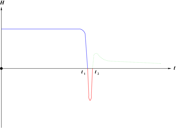
Figure 10: The expansion rate $H(t)$ during inflation (blue), deflation (red), and                          subsequent expansion (green). The graph is not properly scaled.

Besides allowing for equations of state with $w<-1$, a brief period of deflation furnishes a most natural mechanism for the reheating of the universe after a long period of inflation.

The kind of post-deflationary regime that emerges needs careful analysis. Although a succession of inflation to deflation cycles cannot be excluded, the asymptotic geometry must satisfy:

$$t\gg t_{2}\quad\Longrightarrow\quad H(t)=\ {\dot{b}}\,(t)\ >\ 0\;\;.$$ (174)

This is a direct consequence of the superior stength of the thermal screening effect relative to the causal volume increase. A small power law expansion, like radiation, is an acceptable post-deflationary geometry. In Figure 10, where the time evolution of $H(t)$ during inflation and deflation is exhibited, such a geometry has been assumed afterwards and is indicated by the dotted line.

5 Epilogue

A very important and desirable property of the cosmological evolution described herein, is its naturalness. $\Lambda$-driven inflation converts a problem – the presence of a huge bare cosmological constant in the effective theory – into a virtue. It completely avoids the problem that starting scalar-driven inflation requires a vanishingly improbable homogeneous fluctuation over more than a horizon volume [5].

The quantum gravitational back-reaction to inflationary particle production offers an attractive mechanism for stopping $\Lambda$-driven inflation. It obviates the need for fine tuning by making the long duration of inflation a trivial consequence of the fact that gravity is a weak interaction, even at scales $M\sim 10^{16}GeV$. This same fact serves to explain why the induced pressure must be nearly minus the induced energy density. The sign of the effect follows from the fact that gravity is attractive.

Back-reaction certainly slows inflation by an amount which eventually becomes non-perturbatively large [6]. The problem has long been evolving this highly attractive model beyond the breakdown of perturbation theory to the current epoch. In this paper, we have developed a technique for accomplishing this. The first key idea is that, even when the net screening effect becomes large, its instantaneous rate of increment is always small. Therefore, it can be computed perturbatively. The second key idea is to follow Starobinsky [10] in subsuming the non-perturbative aspects of back-reaction into a stochastic background whose evolution obeys the classical field equations.

The screening effect at any point derives from the coherent superposition of interactions from within the past lightcone of that point. Since the invariant volume of the past lightcone actually grows faster as the expansion rate slows, screening must overcompensate the bare cosmological constant and lead to a period of deflation. Were the physics completely classical and stable, this period of deflation would never end. What allows the universe to recover is the formation of a thermal barrier of the most recently created particles. This barrier scatters the virtual infrared quanta needed to propagate the screening effect out from the period of inflationary particle production. Because the thermal barrier becomes hotter and denser as deflation progresses, this scattering process must very quickly arrest deflation and allow slower expansion to resume. That, in turn, dilutes the thermal barrier, and the subsequent evolution is controlled by the balance between the growth of the visible portion of the period of inflationary particle production and the persistence of the thermal barrier. It is clear that dynamical stability against uncontrollable expansion or contraction has been achieved (see Figure 11).

Figure 11: The physical effects that prevent instabilities under time evolution.

As far as the construction of a cosmological model is concerned, there are some issues that should be addressed:
– During inflation, the model presented is realistic since it was entirely based on the graviton. In the post-inflationary analysis, the graviton-like scalar was used to facilitate the explicit computations. Nonetheless, the main conclusion – the existence of a short period of deflation – is universal. The same is true for the physical role of the various modes: the infrared modes carry correlations from the inflationary regime to later times and provide the dominant contribution to the quantum induced stress tensor, the thermal modes decrease the number of infrared modes present by scattering with them, and the ultraviolet modes appear only as virtual particles. What will most certainly differ is the explicit form of the infrared decay rate and induced stress. For a realistic cosmology, these computations should be repeated using the effective gravitational theory (1) and the resulting post-deflationary geometry should be determined. Within the same context, since the era of deflation furnishes a very natural mechanism for reheating, the corresponding temperature should be evaluated.
– The dynamical principle which determines evolution is the balance between the two restoring forces of Figure 11. As long as the expansion – or contraction – of spacetime is very rapid, gravitation dominates. Matter becomes important when the expansion rate does not dominate over a typical matter reaction time. The desired post-deflationary regime is that of radiation. The transition to a matter dominated universe follows naturally. Between every pair of successive transitions, there is a period of varying imbalance or, equivalently, of varying screening of $\Lambda$. If the recently observed data supporting an accelerated expansion [1] persists, it could be the result of a corresponding imbalance in the dynamical stability of the system a while after the transition to matter domination. Whether such behaviour occurs, can be determined from the time evolution of the expansion rate and the deceleration parameter. Because our parameter space is very small, it should be possible to obtain predictive expressions for these quantities.
– During the short period of deflation, violations of the weak energy condition are allowed and “exotic” equations of state satisfying $w<-1$ become feasible. It is worthwhile to investigate whether such a phenomenon could leave its signature in specific observational measurements [19].
– A requirement on the model is its consistency with the measured spectrum of the cosmic microwave background radiation [3]. Although a detailed analysis of the evolution of the primordial density perturbations within the proposed framework is missing, it seems that – if the inflation to deflation transition is sudden and the duration of contraction is small – the spectrum is not altered in any significant way [20].

Finally, the “phase space” of our basic assumptions should be reviewed:
– Perturbation theory validity: Perturbative corrections do become strong but not because each elementary interaction gets to be strong – as is the case, for instance, in QCD. Here, each elementary interaction is always weak. Corrections become strong by the coherent superposition of inherently weak processes as their number vastly increases with time. Perturbation theory breaks in a very soft way because when the dominant term gets to be strong, all higher order terms are still weak [18]. Except for a small interval around the transition, perturbation theory is valid throughout and its leading part provides the main physical effect.
– De Sitter spacetime validity: If we assume a generic power law $a(t)=t^{s}$, there is a lower bound on the power $s$ coming from measurements of the spectral index $n=1-2s^{-1}$ [21]. The bound is $s>20$ and the exponential is a superb approximation to such a high power law.
– Spacetime dimensionality: Modulo exceptional cases, an extra dimension is equivalent – from a four-dimensional perspective – to a particle spectrum. A general spectrum was studied and the graviton emerged as the unique known particle that participates dominantly to the effects. A scalar could contribute as well if its mass is substantially lower than the natural scale and if its dynamics is not described by (28). Furthermore, the parameter space of such a scalar must be restrictive enough to allow predictions; otherwise, the (higher-dimensional) theory it resides in cannot be fundamental.
– Supersymmetry: All the analysis is completely independent of supersymmetry. It is, therefore, valid for any supersymmetric theory both in its unbroken and – the physically unavoidable – broken regime.

Acknowledgements

This work was partially supported by European Union grants HPRN-CT-2000-00122 and HPRN-CT-2000-00131, by the DOE contract DE-FG02-97ER41029, and by the Institute for Fundamental Theory at the University of Florida.

References

-
[1]
A. G. Reiss et al.,
Astron. J. 116 (1998) 1009,
arXiv:astro-ph/9805201.
S. Perlmutter et al., Astrophys. J. 517 (1999) 565, arXiv:astro-ph/9812133. - [2] A. D. Linde, Particle Physics and Inflationary Cosmology (Harwood, Chur, Switzerland, 1990).
- [3] P. de Bernardis et al., Astrophys. J. 564 (2002) 559, arXiv:astro-ph/0105296.
-
[4]
L. Abbott and S. Deser,
Nucl. Phys. B195 (1982) 76.
P. Ginsparg and M. J. Perry, Nucl. Phys. B222 (1983) 245. - [5] T. Vachaspati and M. Trodden, Phys. Rev. D61 (2000) 023502, arXiv:gr-qc/9811037.
- [6] N. C. Tsamis and R. P. Woodard, Nucl. Phys. B474 (1996) 235, arXiv:hep-ph/9602315 ; Ann. Phys. 253 (1997) 1, arXiv:hep-ph/9602316.
- [7] N. C. Tsamis and R. P. Woodard, Phys. Rev. D57 (1998) 4826, arXiv:hep-ph/9710444.
- [8] L. R. Abramo, N. C. Tsamis and R. P. Woodard, Fortschr. Phys. 47 (1999) 389, arXiv:astro-ph/9803172.
- [9] N. C. Tsamis and R. P. Woodard, Phys. Lett. B426 (1998) 21, arXiv:hep-ph/9710466.
- [10] A. A. Starobinsky and J. Yokoyama, Phys. Rev. D50 (1994) 6357, arXiv:astro-ph/9407016.
-
[11]
A. Vilenkin and L. H. Ford,
Phys. Rev. D26 (1982) 1231.
A. D. Linde, Phys. Lett. B116 (1982) 335.
A. A. Starobinsky, Phys. Lett. B117 (1982) 175. - [12] L. H. Ford, Phys. Rev. D31 (1985) 710.
- [13] L. R. Abramo and R. P. Woodard, Phys. Rev.D65 (2002) 063516, arXiv:astro-ph/0109273.
- [14] V. K. Onemli and R. P. Woodard, Class. Quant. Grav. 19 (2002) 4607, arXiv:gr-qc/0204065.
-
[15]
J. Schwinger,
J. Math. Phys. 2 (1961) 407.
L. V. Keldysh, Sov. Phys. JETP 20 (1964) 1018. - [16] J. Iliopoulos, T. N. Tomaras, N. C. Tsamis and R. P. Woodard, Nucl. Phys. B534 (1998) 419, arXiv:gr-qc/9801028.
- [17] S. W. Hawking and G. F. R. Ellis, The Large Scale Structure of Space-Time (Cambridge, Cambridge, Great Britain, 1973).
- [18] N. C. Tsamis and R. P. Woodard, Phys. Rev. D57 (1998) 4826, arXiv:hep-ph/9710444.
-
[19]
Y. Wang,
Astrophys. J. 531 (2000) 676,
arXiv:astro-ph/9806185.
http://snap.lbl.gov - [20] F. Finelli and R. Brandenberger, Phys. Rev. D65 (2002) 103522, arXiv:hep-th/0112249.
- [21] Latest MAP results (http://map.gsfc.nasa.gov).