Testing resummed NLO-BFKL kernels

Abstract

We propose a new method to test the (resummed) next-to-leading-order BFKL evolution kernels using the Mellin transformed $j$-moments of the proton structure function $F_{2}.$

1 How to test BFKL evolution equations?

The Balitsky Fadin Kuraev Lipatov (BFKL) evolution equation [1], derived in the framework of perturbative QCD, has held the attention of the scientific community since a long time. The summation of leading logarithms of energy in the perturbative expansion gives valuable tools for the investigation of deep-inelastic scattering at small $x_{Bj}$ (equivalently large energy squared $W^{2}\sim Q^{2}/x_{Bj}$). Indeed, the first experimental results from HERA confirmed the existence of a strong rise of the proton structure function $F_{2}$ with energy in agreement with the trends implied by the solution of the BFKL equation. It has been possible [2] to describe the old data at small $x_{Bj}$ and in a certain range of $Q^{2}.$ However the price to pay was to get a phenomenological value of the intercept (the exponent of $1/x_{Bj}$ in the BFKL formula, see later in the text) less than the predicted range (the corresponding value of the strong coupling constant is $\alpha_{s}\sim.1$ instead of $\sim.2$). This was revealing the need for rather sizable higher order corrections.

At the next-to-leading log level, these corrections have been calculated after much efforts [3] and appeared to be so large that they overshoot the expected phenomelogical effect and could even invalidate the whole approach. Soon after, it was realized [4] that the main problem came from the existence of spurious singularities which ought to be cancelled by an appropriate resummation at all orders of the perturbative expansion. This is required by the QCD renormalization group. Indeed, various resummation schemes have been proposed [4, 5, 6] which satisfy the renormalization group requirements while retaining the exact value of the next-leading log term in the BFKL kernel computed in Refs.[3]. Hence, the constraints can be satisfied and the next-to-leading order introduced without destroying the whole scheme.

However, the resummation schemes possess some ambiguity, since higher order logs (beyond the next-to-leading ones) are not known. Such variations appear, e.g. in Ref.[4], where four different resummation schemes have been proposed. These schemes, denoted scheme 1,…4 in the following, will be the subject of our present study. Other schemes have been proposed [5, 6] and will be studied as well later [7]. It is worth to confront these various schemes with data, to check their validity and distinguish between different resummation options.

Precise phenomenological tests of QCD evolution equations are one of the main goals of deep inelastic scattering phenomenology. For DGLAP evolution [8], it has been possible to test it in various ways with next-to-leading log $Q^{2}$ (NLO) corrections and it works quite well in a large range of $Q^{2}.$ Testing precisely BFKL evolution beyond leading order is much more difficult. The main problem is the complicated mismatch between QCD perturbative and non perturbative inputs, since the corresponding factorization properties, i.e. $k_{T}$ factorization [9], are more involved than for DGLAP evolution. A way out could be to stay within the perturbative regime by using only massive or highly virtual colliding particles, like $\gamma^{*}\!-\!\gamma^{*}$ scattering, but the data are yet too imprecise that no definite conclusion can be drawn. Note also that some perturbative QCD ingredients (such as the so-called “impact factors”) are not yet but will be soon available [10].

In the present paper, we propose a method for testing the (resummed) BFKL predictions for the proton structure functions, via a transformation to Mellin space.

On the one hand, the present set of data allows for a precise determination of the Mellin transform of $F_{2}$ in a large range of $Q^{2}$ and $j,$ the Mellin conjugate of $x_{Bj},$ considered as a continuous variable. On the other hand, the BFKL predictions at leading order and beyond are easier to formulate in Mellin space since one can obtain tests of the evolution kernels which are essentially dependent on the calculable perturbative part. In our formulation, we assume that $k_{T}$ factorization remains valid for the resummed kernel. An improved formulation of $k_{T}$ factorization containing the NLO $\gamma^{*}$ impact factors when they will be available, will allow to refine our study in the future.

The proposed method has the following features. It treats in parallel both LO and (resummed) NLO BFKL kernels. It uses a $k_{T}$ factorized formulation of the structure functions which includes the factorized Green function solution derived in Ref. [5]. The present essay is of introductory nature, and present a first, non sophisticated, phenomenological investigation of the proton structure functions [11, 12], where we compare the LO-DGLAP GRV parametrization [13] of proton structure functions with the BFKL kernel predictions. In a forthcoming publication [7], we shall give an extensive and more systematic study using our method.

The plan of contents is organized as follows; In the next section, we start by expressing the LO BFKL predictions in Mellin space, defining three characteristic relations. In section 3 we elaborate the corresponding set of predictions for the resummed NLO-BFKL kernels. An application to the DGLAP/BFKL comparison is presented in section 4. Section 5 provides a conclusion and an outlook on future work.

2 BFKL predictions in Mellin space

The formulation of the proton structure functions in the (LO) BFKL approximation can be expressed as follows [2]:

$$\pmatrix{F_{T}\cr F_{L}\cr G}=\int\frac{d\gamma}{2i\pi}\left(\frac{Q^{2}}{Q_{0}^{2}}\right)^{\gamma}e^{\frac{\alpha_{s}N_{c}}{\pi}\chi_{L0}(\gamma)\ln\left({1}/{x_{Bj}}\right)}\pmatrix{h_{T}\cr h_{L}\cr 1}\omega(\gamma)$$ (1)

where one has written the BFKL kernel as

$$\chi_{L0}(\gamma)=2\psi(1)-\psi(\gamma)-\psi(1-\gamma)\ .$$ (2)

In formula (1), with conventional notations, $F_{T},F_{L},G$ stand respectively for transverse , longitudinal and gluon structure functions, $\alpha_{s}$ is the (fixed) coupling constant, $\omega(\gamma)$ is an (unknown) non-perturbative coupling to the proton while

$$\pmatrix{h_{T}\cr h_{L}}=\frac{\alpha_{s}}{3\pi\gamma}\frac{(\Gamma(1-\gamma)\Gamma(1+\gamma))^{3}}{\Gamma(2-2\gamma)\Gamma(2+2\gamma)}\frac{1}{1-\frac{2}{3}\gamma}\pmatrix{(1+\gamma)(1-\frac{\gamma}{2})\cr\gamma(1-\gamma)}\ ,$$ (3)

correspond to the known perturbative couplings to the photon, usually called LO “impact factors” in the literature. Note that, in the framework of $k_{T}$ factorization, $\gamma$ plays the rôle of a “running” anomalous dimension, whose physical value is determined by the integration of (1). As already mentionned in the introduction, formula (1) gives rise to an interesting effective BFKL phenomenology [2] in the small $x_{Bj}$ region, but it has to rely on the parametrization of the unknown non perturbative function $\omega(\gamma)$ and leads to values of $\alpha_{s}$ quite smaller than expected.

Mellin-transforming (1) in $j$-space, one easily finds

$$\pmatrix{\tilde{F}_{T}\cr\tilde{F}_{L}\cr\tilde{G}}=\int\frac{d\gamma}{2i\pi}\left(\frac{Q^{2}}{Q_{0}^{2}}\right)^{\gamma}\frac{1}{j-1-\frac{\alpha_{s}N_{c}}{\pi}\chi_{L0}(\gamma)}\pmatrix{h_{T}\cr h_{L}\cr 1}\omega(\gamma)\ .$$ (4)

Looking for the poles in $\gamma,$ it is straightforward to use the residue formula and get

$$\!\pmatrix{\tilde{F}_{T}\cr\tilde{F}_{L}\cr\tilde{G}}=\sum_{i}\frac{1}{\frac{\alpha_{s}N_{c}}{\pi}[-\chi_{L0}^{\prime}(\gamma_{i}(j))]}\left(\frac{Q^{2}}{Q_{0}^{2}}\right)^{\gamma_{i}(j)}\!\pmatrix{h_{T}(\gamma_{i}(j))\cr h_{L}(\gamma_{i}(j))\cr 1}\ \omega(\gamma_{i}(j))$$ (5)

where $\gamma_{i}(j)$ are the ($\gamma_{i}<1/2$) roots of the equation

$$j-1=\frac{\alpha_{s}N_{c}}{\pi}\chi_{L0}(\gamma_{i}(j))\ .$$ (6)

In fact, with good accuracy at large enough $Q^{2},$ (comparable to the leading twist approximation in DGLAP evolution), one can only retain the rightmost pole $\gamma_{1}(j).$ We are thus left with the following simple formula as a starting point of our analysis:

$$\pmatrix{\tilde{F}_{T}\cr\tilde{F}_{L}\cr\tilde{G}}\approx\frac{1}{\frac{\alpha_{s}N_{c}}{\pi}[-\chi_{L0}^{\prime}(\gamma_{1}(j))]}\left(\frac{Q^{2}}{Q_{0}^{2}}\right)^{\gamma_{1}(j)}\pmatrix{h_{T}(\gamma_{1}(j))\cr h_{L}(\gamma_{1}(j))\cr 1}\ \omega(\gamma_{1}(j))\ .$$ (7)

From equation (7), three model-independent predictions, i.e. independent of non-perturbative assumptions, can be drawn:

i) The Mellin transform of $F_{2}\equiv F_{T}+F_{L}$ should verify:

$$\ln\tilde{F}_{2}(j,{Q^{2}})=\gamma_{1}(j)\ln({Q^{2}})+f(j)$$ (8)

in some range of $j$ near $1$ where the BFKL equation is expected to be relevant. The function $f(j)$ regroups all $Q^{2}$-independent terms in (7).

ii) $\gamma_{1}(j),$ extracted from (7) as the slope in $\ln({Q^{2}}),$ should verify the equation (6) for the anomalous dimension, namely

$$\chi_{L0}(\gamma_{1}(j))\equiv\frac{\pi}{\alpha_{s}N_{c}}\ (j\!-\!1)\ ,$$ (9)

with constant ${\alpha_{s}},$ and $\chi_{L0}$ given by (2).

iii) The gluon structure function (one may also choose the obervable $F_{L}$) should verify, via Mellin transform:

$$\ln(\tilde{G}(j,Q^{2}))=\ln\left(\tilde{F_{2}}(j,Q^{2})\right)-\gamma_{1}(j)\ \ln\left(h_{T}+h_{L}\right)\ .$$ (10)

The predictions (8), (9) (10) represents a stringent set of constraints which have to be verified by the Mellin-transformed of the proton structure functions in a region $j$ near 1. In fact we will confirm that the (LO) BFKL kernel does not pass this step.

3 Resummed NLO-BFKL predictions in Mellin space

Interestingly, using a reasonable $k_{T}$ factorized ansatz, the predictions i)-iii) remain valid for NLO-BFKL resummation kernels, up to specific modifications due to the running of the coupling constant.

Let us formulate the (resummed) NLO-BFKL structure functions in Mellin space as follows:

$$\pmatrix{\tilde{F}_{T}\cr\tilde{F}_{L}\cr\tilde{G}}=\int\frac{d\gamma}{2i\pi}\left(\frac{Q^{2}}{\Lambda_{QCD}^{2}}\right)^{\gamma}e^{-\frac{1}{b(j\!-\!1)}\ X(\gamma,j)}\pmatrix{h_{T}\cr h_{L}\cr h_{G}}\eta(\gamma)\ ,$$ (11)

where, by definition

$${\partial\over\partial\gamma}X(\gamma,j)\equiv\chi_{NLO}(\gamma,j)\ .$$ (12)

The function $X(\gamma,j)$ appears in the solution of the Green function derived from the renormalization-group improved small-$x_{Bj}$ equation [5], $\chi_{NLO}(\gamma,j)$ is the resummed NLO-BFKL kernel and $b=11-2/3\ N_{f}/N_{c}$ defines the running of the coupling constant

$$\frac{N_{c}}{\pi}\ \alpha_{s}(Q^{2})=\frac{1}{b\ln\left(Q^{2}/\Lambda_{QCD}^{2}\right)}\ .$$ (13)

Before going further, let us comment formula (11). This formula captures the (large) $Q^{2}$-dependent part of the gluon Green function which has been shown to have factorization properties [5]. In fact the non perturbative contribution has been factorized out in the function $\eta(\gamma).$ Some unknown $Q^{2}$-dependence may still remain in the NLO contributions to the impact factor vector $(h),$ which we neglected in the present analysis.

Starting from this ansatz, let us derive the NLO constraints similar to (8)-(10). At large enough $Q^{2}/\Lambda_{QCD}^{2},$ one can use the saddle-point appoximation to evaluate (11). Assuming that the perturbative impact factors and the non-perturbative function $\eta$ do not vary much, the saddle-point condition reads

$$j\!-\!1\sim\frac{1}{b\ \ln\left(Q^{2}/\Lambda_{QCD}^{2}\right)}\ \chi_{NLO}(\bar{\gamma},j)=\frac{N_{c}\ \alpha_{s}(Q^{2})}{\pi}\ \chi_{NLO}(\bar{\gamma},j)\ ,$$ (14)

where $\bar{\gamma}(j,Q^{2})$ is the saddle-point value. Relation (14) is nothing else than the NLO extension of condition ii) of (9) to the case of a running coupling constant (13).

Inserting the saddle point defined by (14) in formula (11), one obtains the new set of constraints at NLO level as follows:

i) The Mellin transform of $F_{2}\equiv F_{T}+F_{L}$ verifies:

$${\partial\over\partial\ln({Q^{2}})}\ln\tilde{F}_{2}(j,{Q^{2}})\ \sim\ \bar{\gamma}(j,Q^{2})$$ (15)

where $\bar{\gamma}(j,Q^{2})$ is now a smoothly $Q^{2}$-dependent effective anomalous dimension defined by the following property.

ii) $\bar{\gamma}(j,Q^{2})$ verifies the anomalous dimension equation, namely

$$\chi_{NLO}(\bar{\gamma}(j,Q^{2}))\equiv\frac{\pi}{\alpha_{s}(Q^{2})N_{c}}\ (j\!-\!1)\ ,$$ (16)

where $\chi_{NL0}$ is one of the resummed NLO-BFKL candidate kernels proposed in the literature.

iii) The gluon structure function (one may also choose the obervable $F_{L}$) verifies, via Mellin transform:

$$\ln(\tilde{G}(j,Q^{2}))=\ln\left(\tilde{F_{2}}(j,Q^{2})\right)-\bar{\gamma}(j,Q^{2})\ \ln\left[h_{T}(\bar{\gamma})+h_{L}(\bar{\gamma})\right]\ ,$$ (17)

where NLO effects of impact factors are neglected.

The interest of the relations (15) (16) (17) is that they are formally similar with the LO ones by the direct substitution of the LO kernel by the NLO ones and of a fixed coupling constant by the running one at one-loop. They are only approximate, since they rely on a saddle-point approximation which may not be always justified (see [5] for a discussion). However, in the present context, the validity of the saddle-point approximation can be tested directly from the phenomenological analysis. Due to the observed smoothness of the Mellin transforms, we do not expect large corrections to the saddle-point results.

4 Application: the “proximity” between DGLAP and NLO-BFKL

In this section, we want to check the reliability of the Mellin space method by a study of DGLAP parametrizations of the data [11] . It is well-known that DGLAP parametrizations fit well the data in a large range of $x_{Bj}$ and $Q^{2}>1\ GeV.$ Choosing such a parametrization of structure functions, namely the GRV set of structure functions [13], we are able to Mellin transform them easily, and thus discuss the comparison between DGLAP and LO/NLO BFKL evolution equations. DGLAP evolution is automatically obeyed by the input functions and we want to compare them with BFKL evolution using relations (8) (9) (10) for LO and (15) (16) (17) for NLO. The physical question we ask in this application is whether or not there may exist a compatibility between DGLAP and BFKL evolution equations.

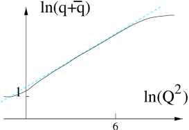
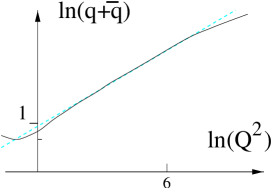
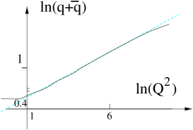
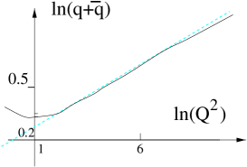
Figure 1: Evolution of the Mellin transformed ${(q+\bar{q})}(j)$ as a function of $Q^{2}.$
From left to right and top to bottom: $j=1.1,1.3,1.4,1.5,1.6,1.8.$

Let us first consider the singlet density distribution in Mellin space $\tilde{\Sigma}\equiv({q\!+\!\bar{q}})(j),$ see Fig.1. It is an easy exercise to obtain it from the input GRV parametrizations [13] and LO DGLAP matrix elements in Mellin space [8].

It is clear from Fig.1 that there exists an interval $1.3\leq j\leq 1.7$ in which the slope of $\ln\tilde{\Sigma}$ as a function of $\ln Q^{2}$ is almost constant. The observed approximate constancy meets the requirement of condition i). We will focus our study to this region which is Mellin-conjugated to the small $x_{Bj}$ region.

Taking into account the anomalous dimension values, it is now straightforward to look for the LO prediction (9) and the various NLO predictions (16) depending on the choice of resummation scheme in [4].

We have displayed in Fig.2 for comparison the results for both the standard (LO) BFKL and for one of the Resummed NLO BFKL schemes (scheme 4). In our application plotting $\chi(\gamma_{i}(j_{i}))$ as a function of $j_{i}$ should give points aligned on a straight line extrapolating to 0 at $j=1.$ The slope gives the (average) value of $\pi N_{C}/\alpha_{s}.$ By simple inspection of Fig.2, it is clear that there is a large difference between LO and NLO (scheme 4 of [4]) results. The LO test completely fails in shape and magnitude, while the NLO test is satisfactory. In this case, the measured slope leads to an average value $\alpha\sim.23$ which is reasonable for the $Q^{2}$ range considered for the structure functions.

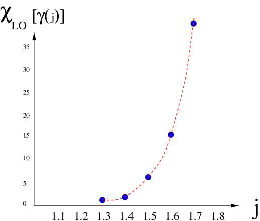
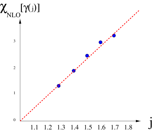
Figure 2: Study of the LO and NLO BFKL kernels in Mellin $j$-space.
Top: (LO) BFKL kernel;
Bottom: Resummed NLO BFKL kernel, scheme 4 of Ref. [4].

Some comments are in order. We have here used a set of structure functions which, on the one hand verifies the DGLAP evolution and, in the other hand give a satisfactory fit of data. The conclusion of our test would be that there is not much difference between DGLAP evolved effective anomalous dimensions from DGLAP evolution and from some well-choosen resummed NLO-BFKL kernels. This remark corroborates the proximity of DGLAP and NLO-BFKL predictions for the gluon anomalous dimension in [5] and, in a different context, the smallness of BFKL-like corrections to the DGLAP evolution equation found in [14] for HERA data.

The new point is that our method allows for sensitive tests of the resummed NLO-BFKL kernels. For instance the schemes 1,2 fail [12] and this is to be related to the fact that not all large logs are resummed [4]. Scheme 3 gives a satisfactory shape but with an averaged $\alpha_{s}\sim.27$ quite too strong. This is for illustration of the sensitiveness of the method.

We postpone to a more systematic study [7] the comparison between different sets of structure functions, different methods, and also the consideration of non-DGLAP parametrizations in order to evaluate the systematic biases which could occur from these different options. We also leave for future study the relations (10),(17) which gave promising results in [11].

5 Conclusion and outlook

• We have proposed a method for confronting with precision “data” the various resummed BFKL kernels with next-to-leading log accuracy. These “data” are the Mellin-transformed of the proton structure function.

• Due to the high precision of modern experimental data on $F_{2}$, we expect the Mellin transform to be well determined, at least in the region of $j$ and $Q^{2}$ needed for the test.

• We make use of a $k_{T}$ factorized formulation of the structure function which grasps the constraints coming from the QCD renormalization group improved small-$x_{Bj}$ equation [5].

• In a first, preliminary, application using the parametrization [13] as input, the method leads with high sensibility to an incompatibility of the LO BFKL kernel while only one of the four resummed NLO BFKL schemes of Ref. [4] shows a compatibility with the DGLAP parametrization of data.

The application we have performed is far from complete, and was only serving as a test of the method sensitivity. Further studies in various interesting directions deserve to be pursued [7]. let us quote some of them.

It is interesting to test whether the present set of data and with which accuracy, the Mellin transformed of the structure functions can be obtained. In particular, it would be useful to see eventual differences between DGLAP and non-DGLAP parametrizations of data, to see whether and where there could be a systematical bias introduced by the DGLAP framework.

Concerning the resummation schemes, the application of the method with the correct NLO accuracy requires to take fully into account the coupling constant running. It is thus required to separate data in small regions of $Q^{2}$ and make the tests separately in each region, in order to follow the $Q^{2}$ evolution of the coupling constant.

We expect to be able to answer these questions soon [7].

References

- [1] L.N.Lipatov, Sov. J. Nucl. Phys. 23 (1976) 642; V.S.Fadin, E.A.Kuraev and L.N.Lipatov, Phys. lett. B60 (1975) 50; E.A.Kuraev, L.N.Lipatov and V.S.Fadin, Sov.Phys.JETP 44 (1976) 45, 45 (1977) 199; I.I.Balitsky and L.N.Lipatov, Sov.J.Nucl.Phys. 28 (1978) 822.
- [2] H Navelet, R.Peschanski, Ch. Royon, S.Wallon, Phys. Lett. B385 (1996) 357. S.Munier, R.Peschanski, Nucl.Phys. B524 (1998) 377.
- [3] V.S. Fadin and L.N. Lipatov, Phys. Lett. B429 (1998) 127; M.Ciafaloni, Phys. Lett. B429 (1998) 363; M. Ciafaloni and G. Camici, Phys. Lett. B430 (1998) 349.
- [4] G.P. Salam, JHEP 9807 (1998) 019
-
[5]
M. Ciafaloni, D. Colferai, G.P.
Salam, Phys.Rev. D60 114036, , JHEP 9910 (1999) 017;
M. Ciafaloni, D. Colferai, G.P. Salam,A.M. Stasto, Phys.Lett. B541 (2002) 314. - [6] Stanley J. Brodsky, Victor S. Fadin, Victor T. Kim, Lev N. Lipatov, Grigorii B. Pivovarov, JETP Lett. 70 (1999) 155.
- [7] R.Peschanski, Ch. Royon, L.Schoffel, to appear.
- [8] G.Altarelli and G.Parisi, Nucl. Phys. B126 18C (1977) 298. V.N.Gribov and L.N.Lipatov, Sov. Journ. Nucl. Phys. (1972) 438 and 675. Yu.L.Dokshitzer, Sov. Phys. JETP. 46 (1977) 641. For a review, see e.g. Yu.L. Dokshitzer, V.A. Khoze, A.H. Mueller, S.I. Troyan, Basics of Perturbative QCD .
- [9] S. Catani, M. Ciafaloni, F. Hautmann, Nucl.Phys. B366 (1991) 135; S. Collins, R.K. Ellis, Nucl.Phys. B360 (1991) 3; E.M. Levin, M.G. Ryskin, Yu.M. Shabelski, A.G. Shuvaev, Sov.J.Nucl.Phys. B53 (1991) 657.
- [10] J. J. Bartels, D. Colferai, S. Gieseke, A. Kyrieleis, Phys.Rev. D66 094017, and references therein.
- [11] J. Salomez, Le modèle des dipôles en QCD perturbative (in French), Saclay preprint T02/147 (2002), Diploma Memoir for the “DEA Rh ne-Alpin, ENS Lyon, France”. Available at: http://www-spht.cea.fr/articles/t02/147/
- [12] J. Salomez, unpublished notes.
- [13] M. Gluck, E. Reya, A. Vogt, Z.Phys. C67 (1995) 433; See M. Gluck, E. Reya, A. Vogt, Eur.Phys.J. C5 (1998) 461, for updated parametrizations.
- [14] R.S. Thorne, Phys.Rev. D60 (1999) 054031;G. Altarelli, R.D. Ball, S. Forte, Nucl.Phys B621 (2002) 359, and references from the same authors therein.