Predictions from the Fritzsch-Type Lepton Mass Matrices

M. Fukugita¹, M. Tanimoto² and T. Yanagida³

¹ Institute for Cosmic Ray Research, University of Tokyo, Kashiwa 277 8582, Japan

² Department of Physics, Niigata University, Niigata 950 2181, Japan

³ Department of Physics, University of Tokyo, Tokyo 113 0033, Japan

Abstract

We revisit the Fritzsch-type lepton mass matrix models confronted with new experiments for neutrino mixings. It is shown that the model is viable and leads to a rather narrow range of free parameters. Using empirical mixing information between $\nu_{e}$ and $\nu_{\mu}$, and between $\nu_{\mu}$ and $\nu_{\tau}$, it is predicted that the mixing angle between $\nu_{e}$ and $\nu_{\tau}$ is in the range $0.04<|U_{13}|<0.20$, consistent with the CHOOZ experiment and the lightest neutrino mass is $0.0004<m_{1}<0.0030$ eV. The range of the effective mass measured in double beta decay is $0.002<\langle m_{ee}\rangle<0.007$ eV.

During the last five years we have experienced dramatic advancement in empirical understanding of the mass and mixing of neutrinos. Most recently, the KamLAND experiment selected the neutrino mixing solution that is responsible for the solar neutrino problem nearly uniquely [1]: we are left with only so-called ‘large-mixing angle solution’ (LMA). We have now good understanding concerning the neutrino mass difference squared and mixing between $\nu_{e}$ and $\nu_{\mu}$ [2], and between $\nu_{\mu}$ and $\nu_{\tau}$ [3]. An interesting constraint has also been placed on mixing between $\nu_{e}$ and $\nu_{\tau}$ from the reactor experiment [4].

Anticipating that neutrinos are all massive from an early indication of the Kamiokande experiment [5], we proposed [6] that neutrino mass and mixing may be described by mass matrices similar to those proposed by Fritzsch for quarks [7]. After the secure confirmation of neutrino oscillation at SuperKamiokande [3], a large number of mass matrix models are proposed [8], but many of them among interesting models lead to bimaximal mixing. We now know that mixing between $\nu_{e}$ and $\nu_{\mu}$ is large but not maximal [2], whereas mixing between $\nu_{\mu}$ and $\nu_{\tau}$ may be maximal [3]. This mixing pattern, together with small mixing between $\nu_{e}$ and $\nu_{\tau}$, is a characteristic embedded in the Fritzsch type matrices we proposed.

So, we revisit the Fritzsch-type mass matrix model to examine whether it is still consistent with all experiments. We find that it is, but the model leads, in particular after the KamLAND experiment, to a narrow allowed parameter range that can be tested in neutrino experiments we expect in the future.

A similar analysis was recently done by Xing [9]. The author, however, fixed the phases that appear in matrices to some arbitrary values. So his result is only a limited representation of the model. In this paper we have exhaustively studied for the allowed parameter space of the model.

The model we proposed in [6] consists of the mass matrices of the charged leptons and the Dirac neutrinos of the form

$$m_{E}=\left(\matrix{0&A_{\ell}&0\cr A_{\ell}&0&B_{\ell}\cr 0&B_{\ell}&C_{\ell}\cr}\right)\ ,\qquad\quad m_{\nu D}=\left(\matrix{0&A_{\nu}&0\cr A_{\nu}&0&B_{\nu}\cr 0&B_{\nu}&C_{\nu}\cr}\right)\ ,$$ (1)

where each entry is complex, and the right-handed Majorana mass matrix

$$M_{R}=M_{0}{\bf I},$$ (2)

where $M_{0}$ is a very large mass. We assume that neutrinos are of the Majorana type. We obtain small neutrino masses $m_{1}$, $m_{2}$ and $m_{3}$ through the seesaw mechanism, as

$$m_{i}=m_{\nu D}^{T}M_{R}^{-1}m_{\nu D}.$$ (3)

The lepton mixing matrix is given by

$$U=U_{\ell}^{\dagger}\ Q\ U_{\nu}$$ (4)

where

$$U_{\ell}(1,1)=\sqrt{\frac{m_{2e}m_{3e}(m_{3e}-m_{2e})}{(m_{2e}+m_{1e})(m_{3e}-m_{2e}+m_{1e})(m_{3e}-m_{1e})}}$$

$$U_{\ell}(1,2)=-\sqrt{\frac{m_{1e}m_{3e}(m_{3e}+m_{1e})}{(m_{2e}+m_{1e})(m_{3e}-m_{2e}+m_{1e})(m_{3e}+m_{2e})}}$$

$$U_{\ell}(1,3)=\sqrt{\frac{m_{1e}m_{2e}(m_{2e}-m_{1e})}{(m_{3e}-m_{1e})(m_{3e}-m_{2e}+m_{1e})(m_{3e}+m_{2e})}}$$

$$U_{\ell}(2,1)=\sqrt{\frac{m_{1e}(m_{3e}-m_{2e})}{(m_{2e}+m_{1e})(m_{3e}-m_{1e})}}$$

$$U_{\ell}(2,2)=\sqrt{\frac{m_{2e}(m_{3e}+m_{1e})}{(m_{2e}+m_{1e})(m_{3e}+m_{2e})}}$$

$$U_{\ell}(2,3)=\sqrt{\frac{m_{3e}(m_{2e}-m_{1e})}{(m_{3e}+m_{2e})(m_{3e}-m_{1e})}}$$

$$U_{\ell}(3,1)=-\sqrt{\frac{m_{1e}(m_{2e}-m_{1e})(m_{3e}+m_{1e})}{(m_{3e}-m_{1e})(m_{3e}-m_{2e}+m_{1e})(m_{2e}+m_{1e})}}$$

$$U_{\ell}(3,2)=-\sqrt{\frac{m_{2e}(m_{2e}-m_{1e})(m_{3e}-m_{2e})}{(m_{3e}+m_{2e})(m_{3e}-m_{2e}+m_{1e})(m_{2e}+m_{1e})}}$$

$$U_{\ell}(3,3)=\sqrt{\frac{m_{3e}(m_{3e}+m_{1e})(m_{3e}-m_{2e})}{(m_{3e}+m_{2e})(m_{3e}-m_{2e}+m_{1e})(m_{3e}-m_{1e})}}$$

$$U_{\nu}(1,1)=\sqrt{\frac{m_{2D}m_{3D}(m_{3D}-m_{2D})}{(m_{2D}+m_{1D})(m_{3D}-m_{2D}+m_{1D})(m_{3D}-m_{1D})}}$$

$$U_{\nu}(1,2)=-\sqrt{\frac{m_{1D}m_{3D}(m_{3D}+m_{1D})}{(m_{2D}+m_{1D})(m_{3D}-m_{2D}+m_{1D})(m_{3D}+m_{2D})}}$$

$$U_{\nu}(1,3)=\sqrt{\frac{m_{1D}m_{2D}(m_{2D}-m_{1D})}{(m_{3D}-m_{1D})(m_{3D}-m_{2D}+m_{1D})(m_{3D}+m_{2D})}}$$

$$U_{\nu}(2,1)=\sqrt{\frac{m_{1D}(m_{3D}-m_{2D})}{(m_{2D}+m_{1D})(m_{3D}-m_{1D})}}$$

$$U_{\nu}(2,2)=\sqrt{\frac{m_{2D}(m_{3D}+m_{1D})}{(m_{2D}+m_{1D})(m_{3D}+m_{2D})}}$$

$$U_{\nu}(2,3)=\sqrt{\frac{m_{3D}(m_{2D}-m_{1D})}{(m_{3D}+m_{2D})(m_{3D}-m_{1D})}}$$

$$U_{\nu}(3,1)=-\sqrt{\frac{m_{1D}(m_{2D}-m_{1D})(m_{3D}+m_{1D})}{(m_{3D}-m_{1D})(m_{3D}-m_{2D}+m_{1D})(m_{2D}+m_{1D})}}$$

$$U_{\nu}(3,2)=-\sqrt{\frac{m_{2D}(m_{2D}-m_{1D})(m_{3D}-m_{2D})}{(m_{3D}+m_{2D})(m_{3D}-m_{2D}+m_{1D})(m_{2D}+m_{1D})}}$$

$$U_{\nu}(3,3)=\sqrt{\frac{m_{3D}(m_{3D}+m_{1D})(m_{3D}-m_{2D})}{(m_{3D}+m_{2D})(m_{3D}-m_{2D}+m_{1D})(m_{3D}-m_{1D})}}$$

where 1-3 refers to generation; $Q$ is a phase matrix written as

$$Q=\left(\matrix{1&0&0\cr 0&e^{i\sigma}&0\cr 0&0&e^{i\tau}\cr}\right)\ ,$$ (7)

which is a reflection of phases contained in the charged lepton mass matrix and the Dirac mass matrix of neutrinos. The phases are neglected in the right-handed neutrinos mass matrix. In the presence of mass hierarchy of the left-handed neutrinos, the effect of phases in the right-handed mass matrix is small, and the inclusion of phases changes the anlysis only little. Since the charged lepton masses are well-known, the number of parameters contained in our model is six: $m_{1D},\ m_{2D},\ m_{3D}$, $\sigma$, $\tau$ and $M_{0}$. These parameters are to be determined by empirical neutrino mass and mixing.

We calculate lepton mixing matrix elements using the exact expressions, but they are written approximately

$$U_{12} \simeq -\left({m_{1}\over m_{2}}\right)^{1/4}+\left({m_{e}\over m_{\mu}}\right)^{1/2}e^{i\sigma}$$ (8)

$$U_{21} \simeq \left({m_{1}\over m_{2}}\right)^{1/4}e^{i\sigma}-\left({m_{e}\over m_{\mu}}\right)^{1/2}$$ (9)

$$U_{23} \simeq \left({m_{2}\over m_{3}}\right)^{1/4}e^{i\sigma}-\left({m_{\mu}\over m_{\tau}}\right)^{1/2}e^{i\tau}$$ (10)

$$U_{32} \simeq -\left({m_{2}\over m_{3}}\right)^{1/4}e^{i\tau}+\left({m_{\mu}\over m_{\tau}}\right)^{1/2}e^{i\sigma}$$ (11)

$$U_{13} \simeq \left({m_{e}\over m_{\mu}}\right)^{1/2}U_{23}+\left({m_{2}\over m_{3}}\right)^{1/2}\left({m_{1}\over m_{3}}\right)^{1/4}$$ (12)

$$U_{31} \simeq \left({m_{1}\over m_{2}}\right)^{1/4}U_{32}$$ (13)

where $(m_{e}/m_{\tau})^{1/2}$ is neglected. Rough characteristics of mixing angles are understood from these expressions.

For our anlysis we take as inputs

$$\Delta m^{2}_{\rm atm}=(1.5-3.9)\times 10^{-3}{\rm eV^{2}},\hskip 14.22636pt\sin^{2}\theta_{\rm atm}\geq 0.92$$ (14)

for $\nu_{\mu}-\nu_{\tau}$ mixing from Super-Kamiokande experiment [3], and

$$\Delta m^{2}_{\rm sol}=(6-8.5)\times 10^{-5}{\rm eV}^{2},\hskip 14.22636pt\sin^{2}\theta_{\rm sol}=0.25-0.4$$ (15)

for $\nu_{e}-\nu_{\mu}$ mixing from KamLAND [1], both at a 90% confidence level.

The KamLAND experiment gives another, but less favoured solution within LMA, i.e., the solution allowed only at a 95% confidence level,

$$\Delta m^{2}_{\rm sol}=(1.4-1.8)\times 10^{-4}{\rm eV}^{2},\hskip 14.22636pt\sin^{2}\theta_{\rm sol}=0.27-0.34$$ (16)

which we call KamLAND-B (we call the best favoured solution (15) KamLAND-A). For this case we take a region allowed at a 95% confidence for the Super-Kamiokande data for $\nu_{\mu}-\nu_{\tau}$ mixing for consistency.

We discuss how the allowed parameter region shrinked after the KamLAND data which determined the mass difference squared to a high accuracy. For a purpose of comparison, we also take the LMA for the $\nu_{e}-\nu_{\mu}$ mixing before the KamLAND data [2]:

$$\Delta m^{2}_{\rm sol}=(3-20)\times 10^{-5}{\rm eV}^{2},\hskip 14.22636pt\sin^{2}\theta_{\rm sol}=0.23-0.41$$ (17)

at a 90% confidence level.

We assume that $m_{3\nu}\gg m_{i\nu}$ for $i=1,2$, i.e., $\Delta m_{\ atm}^{2}\simeq m_{3}^{2}$. We do not assume mass hierarchy between $m_{\nu 1}$ and $m_{\nu 2}$. We do not include the empirical constraint from the CHOOZ experiment for mixing between $\nu_{e}$ and $\nu_{\tau}$ in our analysis. We leave this as a free parameter and examine the result against experiment.

We have exhaustively searched for allowed parameter regions that satisfy empirical mass difference squared and mixing in six dimensional space without any prior conditions.

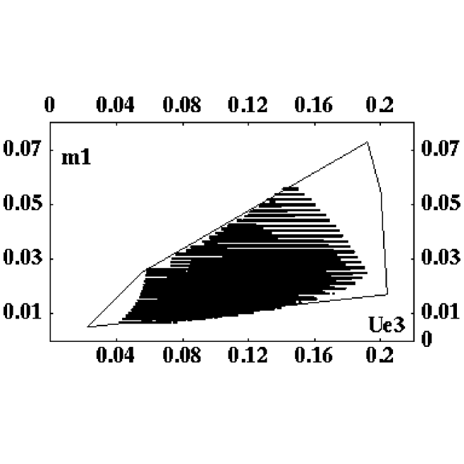
Figure 1: Predicted value of $m_{1}$ in the unit of $m_{3}$ as a function of $|U_{e3}|$ in the case of KamLAND-A. The outer contour shows an allowed region before the KamLAND data are available.

The result is restrictive. We plot in Figure 1 $m_{1}/m_{3}$ as a function of $|U_{e3}|$ for KamLAND-A. The outer contour shows an allowed region before the KamLAND data are available. The model predicts $0.04<|U_{e3}|<0.18$. It is interesting to note that the model upper limit agrees with the empirical constraint from the CHOOZ experiment $|U_{e3}|<0.16$ and that there is a definite lower limit on $|U_{e3}|$. The lightest neutrino mass $m_{1}$ cannot be too small. When $m_{2}$ is used as a unit, $m_{1}/m_{2}=0.05-0.29$ is the allowed range, or $m_{1}=0.0004-0.0030$ eV. Of course, $m_{1}<m_{2}$ is always satisfied because $\theta_{\rm solar}$ does not reach 45^∘.

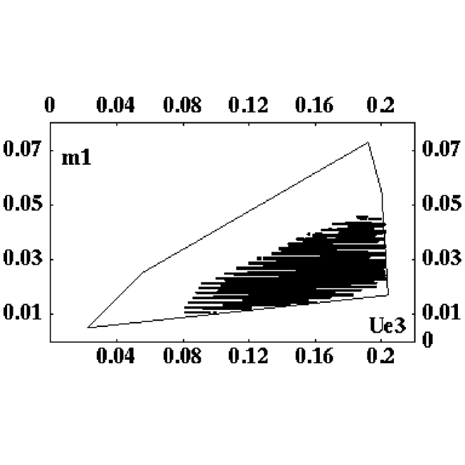
Figure 2: Predicted value of $m_{1}$ in the unit of $m_{3}$ as a function of $|U_{e3}|$ in the case of KamLAND-B. The outer contour shows an allowed region before the KamLAND data are available.

A similar figure is presented for KamLAND-B solution at a 95% confidence level (Figure 2).

The allowed range of the lepton flavour mixing matrix (for KamLAND-A) is given as

$$|U|=\left[\matrix{0.76-0.86&0.50-0.63&0.04-0.19\cr 0.27-0.48&0.63-0.72&0.60-0.71\cr 0.34-0.49&0.42-0.58&0.71-0.80\cr}\right]\ .$$ (18)

This matrix may be compared with a model-independent analysis of neutrino mixing [10], which is modified very little even after the KamLAND experiment. We see general agreement between the two matrices, while the allowed ranges of each matrix element in the present model is quite narrow.

In Figure 3 (Figure 4 for KamLAND-B) we show the rephasing invariant CP violation measure $J_{CP}$ [11], which is defined by

$$J_{CP}={\rm Im}\ [{U_{\mu 3}U^{*}_{\tau 3}U^{*}_{\mu 2}U_{\tau 2}}]\ .$$ (19)

as a function of $|U_{e3}|$.

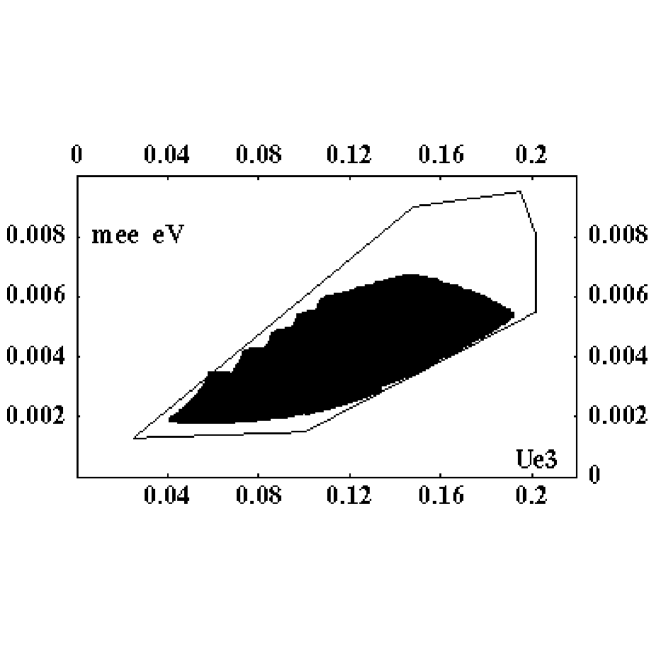
Figure 6: Predicted value of $\langle m_{ee}\rangle$ (eV) as a function of $|U_{e3}|$ in the case of KamLAND-A. The outer contour shows an allowed region before the KamLAND data are available.

Figures 5 and 6 present experimentally more relevant quantities, the CP violating part of neutrino oscillation

$$\Delta P \equiv P(\overline{\nu}_{\mu}\rightarrow\overline{\nu}_{e})-P(\nu_{\mu}\rightarrow\nu_{e})=P(\nu_{\mu}\rightarrow\nu_{\tau})-P(\overline{\nu}_{\mu}\rightarrow\overline{\nu}_{\tau})$$ (20)

$$= P(\overline{\nu}_{e}\rightarrow\overline{\nu}_{\tau})-P(\nu_{e}\rightarrow\nu_{\tau})\ ,$$

and effective mass measured in double beta decay experiment $\langle m_{ee}\rangle$

$$\langle m_{ee}\rangle=m_{1}\ U_{e1}^{2}+m_{2}\ U_{e1}^{2}+m_{3}\ U_{e3}^{2}$$ (21)

for KamLAND-A case. Here, $\Delta P$ is given by

$$\Delta P=4J_{CP}f_{CP}$$ (22)

where

$$f_{CP}\equiv-4\sin\frac{\Delta m^{2}_{21}L}{4E}\sin\frac{\Delta m^{2}_{32}L}{4E}\sin\frac{\Delta m^{2}_{31}L}{4E}\ ,$$ (23)

with $\Delta m_{ij}=m_{i}^{2}-m_{j}^{2}$ and $\Delta P$ is evaluated for $\langle E_{\nu}\rangle=1.3{\rm GeV}$ and $L=295{\rm Km}$, which are parameters for a planned long-baseline neutrino oscillation experiment between the Japanese Hadron Facility (JHF) in Tokai Village (Ibaraki) to the Super-Kamiokande.

Note that the figure of $\langle m_{ee}\rangle$ doe not include the error of $m_{3}$, but fixed at $0.053$ eV. The result should be scaled if actual $m_{3}$ is higher or lower. The effective mass measured in the double beta decay ranges from $2-7$ meV for $m_{3}=0.053$ (eV). The lower limit is raised by a factor of 4 after the KamLAND experiment.

Predictions are summarized in Table 1. We emphasize that interesting features of this model are mixing between $\nu_{e}$ and $\nu_{\mu}$ that is not maximal, unlike in the model proposed in [12] based on the democratic principle or that in the Zee model [13,14], whereas $|U_{13}|$ is automatically predicetd to be small (but non-zero) [8]. Basic features found in experiment seem to be built-in in this model. Without any knowledge for the right-handed neutrino sector, we assumed that the right-handed neutrino mass is proportional to a unit matrix. Modifications for the prediction on the mixing angles are relatively minor even if we somewhat relax this assumption, in so far as the mass hierarchy in the Dirac mass is not disturbed. In conclusion, a simple Fritzsch-type model we proposed in [6] is consistent with all existing neutrino experiments, but the model parameters are now restricted to a narrow range that endows the model with a predicive power.

	$m_{2}/m_{3}$ (input)	$m_{1}/m_{3}$	$|U_{e3}|$	$|J_{CP}|$	$\langle m_{ee}\rangle$ (meV)
KamLAND-A	$0.11-0.19$	$0.007-0.056$	$0.042-0.191$	$\leq 0.021$	$1.9-6.7$
KamLAND-B	$0.18-0.28$	$0.011-0.046$	$0.081-0.202$	$\leq 0.025$	$3.3-8.3$
Before KamLAND	$0.08-0.28$	$0.005-0.073$	$0.025-0.202$	$\leq 0.025$	$1.3-9.5$

Table 1 : Summary of predictions

Acknowledgements

References

[1] KamLAND Collaboration, K. Eguchi et al., hep-ex/0212021.

[2] SNO Collaboration: Q. R. Ahmad et al., Phys. Rev. Lett. 87 (2001) 071301;
nucl-ex/0204008, 0204009.

[3] Super-Kamiokande Collaboration, Y. Fukuda et al., Phys. Rev. Lett. 81 (1998) 1562; J. Kameda, in Proceedings of International Cosmic Ray Conference, Hamburg, 2001, edited by K. H. Kampert, G. Heinzelmann and C. Spiering (Copernicus Gesellschaft, Katlenburg-Lindau, 2001), Vol. 3, p.1057.

[4] CHOOZ Collaboration, M. Apollonio et al., Phys. Lett. 466B (1999) 415.

[5] Kamiokande Collaboration, K.S. Hirata et al., Phys. Lett. 280B (1992) 146.

[6] M. Fukugita, M. Tanimoto, and T. Yanagida, Prog. Theor. Phys. 89 (1993) 263.

[7] H. Fritzsch, Phys. Lett. B73 (1978) 317; Nucl. Phys. B115 (1979) 189.

[8] For a review, see G. Altarelli and F. Feruglio, hep-ph/0206077.

[9] Z.-z. Xing, Phys. Lett. 550B (2002) 178.

[10] M. Fukugita and M. Tanimoto, Phys. Lett. 515B (2001) 30.

[11] C. Jarlskog, Phys. Rev. Lett. 55 (1985) 1039.

[12] M. Fukugita, M. Tanimoto and T. Yanagida, Phys. Rev. D57 (1998) 4429; Phys. Rev. D59 (1999) 113016.

[13] A. Zee, Phys. Lett. 93B (1980) 389; B161 (1985) 141;
L. Wolfenstein, Nucl. Phys. B175 (1980) 92.

[14] S. T. Petcov, Phys. Lett. B115 (1982) 401;
C. Jarlskog, M. Matsuda, S. Skadhauge and M. Tanimoto, Phys. Lett. B449 (1999) 240;
P.H. Frampton and S. Glashow, Phys. Lett. B461 (1999) 95.

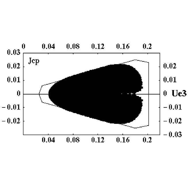
Figure 3: Predicted value of $J_{CP}$ as a function of $|U_{e3}|$ in the case of KamLAND-A. The outer contour shows an allowed region before the KamLAND data are available.

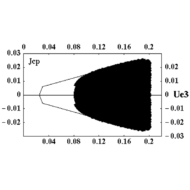
Figure 4: Predicted value of $J_{CP}$ as a function of $|U_{e3}|$ in the case of KamLAND-B. The outer contour shows an allowed region before the KamLAND data are available.

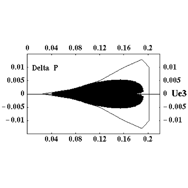
Figure 5: Predicted value of $\Delta P$ as a function of $|U_{e3}|$ in the case of KamLAND-A. The outer contour shows an allowed region before the KamLAND data are available.