Measuring the Relative Strong Phase
in $D^{0}\to K^{*+}K^{-}$ and $D^{0}\to K^{*-}K^{+}$ Decays

Jonathan L. Rosner and Denis A. Suprun

Enrico Fermi Institute and Department of Physics
University of Chicago, Chicago, Illinois 60637

ABSTRACT

In a recently suggested method for measuring the weak phase $\gamma$ in $B^{\pm}\to K^{\pm}(KK^{*})_{D}$ decays, the relative strong phase $\delta_{D}$ in $D^{0}\to K^{*+}K^{-}$ and $D^{0}\to K^{*-}K^{+}$ decays (equivalently, in $D^{0}\to K^{*+}K^{-}$ and $\overline{D}^{0}\to K^{*+}K^{-}$) plays a role. It is shown how a study of the Dalitz plot in $D^{0}\to K^{+}K^{-}\pi^{0}$ can yield information on this phase, and the size of the data sample which would give a useful measurement is estimated.

PACS numbers: 13.25.Ft; 13.25.-k; 14.40.Lb

The relative strong phases for charmed particle decays obey patterns which are not easily anticipated from first principles but are subject to detailed experimental study, for example through the construction of amplitude triangles based on experimentally observed decay rates [1, 2, 3, 4]. It has also been suggested [5, 6, 7] that the final-state phase in the doubly Cabibbo-suppressed decay $D^{0}\to K^{+}\pi^{-}$ may not be the same as that in the Cabibbo-favored decay $D^{0}\to K^{-}\pi^{+}$, even though they should be equal in the flavor-SU(3) limit [8]. Methods for measuring their difference have been proposed [9, 10]. A Dalitz-plot method for measuring the corresponding phase difference in $D^{0}\to K^{*+}\pi^{-}$ and $D^{0}\to K^{*-}\pi^{+}$ makes use of the interference between $K^{*+}$ and $K^{*-}$ bands in $D^{0}\to K_{S}\pi^{+}\pi^{-}$ and is compatible with zero strong phase difference [11, 12].

Recently the question has been raised of the relative strong phase $\delta_{D}$ between $D^{0}\to K^{*+}K^{-}$ and $D^{0}\to K^{*-}K^{+}$ decays (equivalently, in $D^{0}\to K^{*+}K^{-}$ and $\overline{D}^{0}\to K^{*+}K^{-}$) [13]. This phase is important in a proposed method for measuring the weak phase $\gamma$ in the $B^{\pm}\to(KK^{*})_{D}K^{\pm}$ decays. In the present note we point out that $\delta_{D}$ may be measured very directly through the interference of $K^{*+}$ and $K^{*-}$ bands in $D^{0}\to K^{+}K^{-}\pi^{0}$ decays [14]. We discuss the size of present and anticipated samples of this final state and indicate the attainable experimental precision for $\delta_{D}$.

We follow the notations of Ref. [13] and define the $D$ decay amplitudes

$$A_{D}\equiv A(D^{0}\to K^{-}K^{*+}),\ \ \ \bar{A}_{D}\equiv A(\overline{D}^{0}\to K^{-}K^{*+}),$$ (1)

and their ratio

$$\frac{\bar{A}_{D}}{A_{D}}=r_{D}e^{i\delta_{D}}.$$ (2)

The weak phase of $\overline{D}^{0}\to K^{-}K^{*+}$ is negligible, so the CP conjugate amplitude is $A(D^{0}\to K^{+}K^{*-})=\bar{A}_{D}$. We further define

$$A^{\prime}_{D}\equiv A(D^{0}\to K^{-}\,(K^{+}\pi^{0})_{K^{*+}}),\ \ \ \bar{A^{\prime}}_{D}\equiv A(D^{0}\to K^{+}\,(K^{-}\pi^{0})_{K^{*-}}).$$ (3)

The amplitudes of the $K^{*+}\to K^{+}\pi^{0}$ and $K^{*-}\to K^{-}\pi^{0}$ decays are equal. Then the ratio of the amplitudes in (3) is

$$\frac{\bar{A^{\prime}}_{D}}{A^{\prime}_{D}}=\frac{\bar{A}_{D}}{A_{D}}=r_{D}e^{i\delta_{D}}.$$ (4)

Two channels of $D^{0}\to K^{+}K^{-}\pi^{0}$ go through a resonant decay of an intermediate $K^{*+}$ or $K^{*-}$. They fill two bands in the Dalitz plot (see Fig. 1). The width of these bands is determined by the full width $\Gamma\equiv\Gamma_{K^{*\pm}}=(50.8\pm 0.9)$ MeV [15]. Namely, the left vertical line corresponds to $m^{2}_{K^{+}\pi^{0}}=(m_{K^{*+}}-\Gamma/2)^{2}$, while the right one corresponds to $m^{2}_{K^{+}\pi^{0}}=(m_{K^{*+}}+\Gamma/2)^{2}$. Analogous expressions determine the values of $m^{2}_{K^{-}\pi^{0}}$ along the bottom and top borders of the horizontal band. For now we will neglect the actual Breit-Wigner distribution of event density across the bands. Instead, we will assume that the resonant decays are equally likely to appear near the central line of a band and near its borders. We will also assume that the resonant decays do not fall in the regions outside the two bands. We will neglect other resonant decays with smaller branching ratios that are not yet detected but may contribute to the Dalitz plot, such as $D^{0}\to\pi^{0}\,(K^{+}K^{-})_{\phi}$ $D^{0}\to\pi^{0}\,(K^{+}K^{-})_{a_{0}}$, $D^{0}\to\pi^{0}\,(K^{+}K^{-})_{f_{0}}$, $D^{0}\to K^{-}\,(K^{+}\pi^{0})_{K^{*}_{0}(1430)^{+}}$, and $D^{0}\to K^{-}\,(K^{+}\pi^{0})_{\kappa(800)^{+}}$. Some of them are discussed later in the text and in Appendix B. Non-resonant decays uniformly fill the allowed phase space and provide a small background. For simplicity of the argument we will neglect it as well.

Figure 1: The Dalitz plots of the $D^{0}\to K^{+}K^{-}\pi^{0}$ decay. Top panel: constructive interference ($\cos\delta_{D}=1$), 113 events in the square region; bottom panel: destructive interference ($\cos\delta_{D}=-1$), 4 events in the square region. The total number of events in the bands is $N=1500$ in both cases.

The square at the intersection of the bands is the region where two channels interfere with each other. We denote $\epsilon$ to be the fraction of $D^{0}\to K^{-}\,(K^{+}\pi^{0})_{K^{*+}}$ decays that fall into the square region. This fraction only depends on masses and spins of particles involved in the process and the width $\Gamma=\Gamma_{K^{*\pm}}$. So, the probability of a $D^{0}\to K^{+}\,(K^{-}\pi^{0})_{K^{*-}}$ decay falling into the square region is $\epsilon$ as well. This probability is calculated in Appendix A: $\epsilon\approx 0.039$.

Now we can write the number of decays detected in the square region of the Dalitz diagram:

$$N_{s}\propto|\sqrt{\epsilon}A^{\prime}_{D}+\sqrt{\epsilon}\bar{A^{\prime}}_{D}|^{2}=\epsilon\,(1+2r_{D}\cos\delta_{D}+r_{D}^{2})\,|A^{\prime}_{D}|^{2}\ \ ,$$ (5)

while the rest of the resonant decays contribute to the bands outside the square region:

$$N_{out}\propto(1-\epsilon)\,(|A^{\prime}_{D}|^{2}+|\bar{A^{\prime}}_{D}|^{2})=(1-\epsilon)\,(1+r_{D}^{2})\,|A^{\prime}_{D}|^{2}\ \ ,$$ (6)

so that the total number of the events detected in the bands is

$$N=N_{s}+N_{out}\propto(1+2\epsilon r_{D}\cos\delta_{D}+r_{D}^{2})\,|A^{\prime}_{D}|^{2}\ \ .$$ (7)

Experimental measurements of $N_{s}$ and $N$ provide a way of measuring the strong phase $\delta_{D}$:

$$\cos\delta_{D}=\frac{1+r_{D}^{2}}{2\epsilon r_{D}}\,\frac{N_{s}/N-\epsilon}{1-N_{s}/N}\ \ .$$ (8)

The uncertainty in $\epsilon$ can be neglected because it is determined by the uncertainties in particles’ masses and width $\Gamma$, which are small. The ratio $r_{D}$ defined by Eq. (2) can be calculated from the measured branching ratios: ${\cal B}(D^{0}\to K^{+}K^{*-})=(2.0\pm 1.1)\cdot 10^{-3}$ and ${\cal B}(D^{0}\to K^{-}K^{*+})=(3.8\pm 0.8)\cdot 10^{-3}$ [15]. Assuming the uncertainties of these two measurements are uncorrelated, $r_{D}=0.73\pm 0.21$. These values are based on a sample of 35 $D^{0}\to KK^{*}$ decays [16]. For a larger sample, the relative uncertainty in $r_{D}$ will decrease as $1/\sqrt{N}$. Taking the uncertainties of the decay numbers $N_{s}$ and $N$ to be their square roots, we can calculate the uncertainty $\sigma(\cos\delta_{D})$. One can show that the uncertainty in $\cos\delta_{D}$ is mostly determined by the uncertainty in $N_{s}$:

$$\sigma(\cos\delta_{D})\approx\left|\frac{\partial\cos\delta_{D}}{\partial N_{s}}\right|\,\sigma(N_{s})=\frac{(1-\epsilon)\,(1+r_{D}^{2})}{2\epsilon r_{D}}\,\frac{\sqrt{N_{s}/N}}{(1-N_{s}/N)^{2}}\,\frac{1}{\sqrt{N}}\ \ ,$$ (9)

Unlike $\cos\delta_{D}$ itself, the uncertainty of this quantity depends not only on the ratio $N_{s}/N$ but on the total number $N$ of the events detected in the bands as well.

As an aside, note that Eq. (8) predicts a linear dependence of $\cos\delta_{D}$ on $Z\equiv(N_{s}/N)/(1-N_{s}/N)$ with the slope $S=(1-\epsilon)(1+r_{D}^{2})/(2\epsilon r_{D})$. We could alternatively write Eq. (9) as

$$\sigma(\cos\delta_{D})\approx\left|\frac{\partial\cos\delta_{D}}{\partial Z}\right|\,\sigma(Z)\approx S\,\frac{\sqrt{N_{s}/N}}{(1-N_{s}/N)^{2}}\,\frac{1}{\sqrt{N}}\ \ .$$ (10)

The maximum possible value of the ratio $N_{s}/N$ is achieved if the contributions from two bands are fully coherent, i.e., if $\cos\delta_{D}=1$. In this case

$$\frac{N_{s}}{N}=\left(\frac{N_{s}}{N}\right)_{max}=\frac{\epsilon(1+r_{D})^{2}}{1+2\epsilon r_{D}+r_{D}^{2}}=0.074\pm 0.003\ \ .$$ (11)

The minimum possible $N_{s}/N$ is a result of the fully destructive interference at $\cos\delta_{D}=-1$. Then,

$$\frac{N_{s}}{N}=\left(\frac{N_{s}}{N}\right)_{min}=\frac{\epsilon(1-r_{D})^{2}}{1-2\epsilon r_{D}+r_{D}^{2}}=0.0020\pm 0.0035\ \ .$$ (12)

Thus, if $\cos\delta_{D}$ is close to $-1$, one may observe no events in the square region. The source of the uncertainties in the maximum and minimum values of the $N_{s}/N$ ratio is the current 30% error in $r_{D}$ which will be improved as more $D^{0}\to KK^{*}$ decays are detected. Within 1$\sigma$ uncertainty, we can expect the $N_{s}/N$ ratio to lie between $0$ and $0.077$.

Figure 2 shows the contours of constant $\sigma(\cos\delta_{D})$ calculated for this region of $N_{s}/N$ from Eq. (9) for the total number of band events $N$ between 100 and 1500. The uncertainty in $\cos\delta_{D}$ is an increasing function of $N_{s}/N$. So, $\cos\delta_{D}$ will be measured least precisely if it is close to unity. This corresponds to a near maximum value of the $N_{s}/N$ ratio. To estimate the largest uncertainty for different numbers of band events, we calculate how $\sigma(\cos\delta_{D})$ decreases with $N$ when $N_{s}/N$ is fixed at its maximum value of $0.077$:

$$\sigma_{max}(\cos\delta_{D})\approx\frac{8.4}{\sqrt{N}}\ \ .$$ (13)

Figure 2: Contours of $\sigma(\cos\delta_{D})$ for $N_{s}/N$ between $0$ and $0.077$, i.e., for $\cos\delta_{D}$ between $-1.05$ and $1.09$.

Now we discuss the consequences of the fact that the event density across a resonant decay band is not uniform but follows the Breit-Wigner distribution. The differential cross-section for any point on the Dalitz plot (see Appendix A) is

$$\frac{d^{2}\,\Gamma}{dm^{2}_{K^{+}\pi^{0}}\,dm^{2}_{K^{-}\pi^{0}}}\propto\left|\frac{A_{1}(m_{K^{+}\pi^{0}},\,m_{K^{-}\pi^{0}})}{m^{2}_{K^{+}\pi^{0}}-m^{2}_{K^{*+}}+i\,m_{K^{*+}}\Gamma}+\frac{r_{D}e^{i\delta_{D}}\,A_{2}(m_{K^{+}\pi^{0}},\,m_{K^{-}\pi^{0}})}{m^{2}_{K^{-}\pi^{0}}-m^{2}_{K^{*-}}+i\,m_{K^{*-}}\Gamma}\right|^{2}\ \,$$ (14)

The Breit-Wigner factors in the denominators make the population density nonuniform across the bands while the kinematic factors $A_{1}(m_{K^{+}\pi^{0}},\,m_{K^{-}\pi^{0}})$ and
$A_{2}(m_{K^{+}\pi^{0}},\,m_{K^{-}\pi^{0}})$ are responsible for a characteristic emptiness in the middle of the bands. The results of a Monte Carlo simulation of the distribution (14) are shown in Fig. 3.

Figure 3: Two examples of realistic Dalitz plots of the $D^{0}\to K^{+}K^{-}\pi^{0}$ decay. Top panel: constructive interference ($\cos\delta_{D}=1$), 88 events in the square region; bottom panel: destructive interference ($\cos\delta_{D}=-1$), 18 events in the square region. The total number of events in the bands is $N=1500$ in both cases.

We simulated the Dalitz plot distributions 10 times for each of 11 values of $\cos\delta_{D}$ between $-1$ and $1$. For the purposes of these simulations we assumed that $r_{D}$ is equal to its current central value of 0.73. The plot of $Z\equiv(N_{s}/N)/(1-N_{s}/N)$ as a function of $\cos\delta_{D}$ is shown in Fig. 4. To estimate $\sigma(\cos\delta_{D})$ we will assume that the linear relationship between the two quantities still holds. Then, the slope is $S=1/(0.0283\pm 0.0005)=35.3\pm 0.6$ while the maximum value of $N_{s}/N$ is $0.0637\pm 0.0019$ at $\cos\delta_{D}=1$. Both errors are purely statistical Monte Carlo uncertainties. These new values of the slope $S$ and $(N_{s}/N)_{max}$ can be plugged into Eq. (10) to give our best estimate of the maximum uncertainty in $\cos\delta_{D}$: $\sigma(\cos\delta_{D})=(10.16\pm 0.26)/\sqrt{N}$, with the upper bound

$$\sigma_{max}(\cos\delta_{D})\approx\frac{10.4}{\sqrt{N}}\ \ .$$ (15)

Figure 4: $Z\equiv(N_{s}/N)/(1-N_{s}/N)$ as a function of $\cos\delta_{D}$. The solid line with the slope of $0.0283\pm 0.0005$ is the best linear fit to the results of the Monte Carlo simulations. The dash-dotted line is the prediction of the simplified model which doesn’t take into account the Breit-Wigner resonant shapes (Eq. (8)).

Thus, we see that the most precise measurements will be made if $\cos\delta_{D}$ is close to $-1$. The uncertainty of the least precise measurements (in case $\cos\delta_{D}$ is unity) becomes smaller than 0.33 at $N\approx 1000$. Although this uncertainty is rather large, it at least allows one to distinguish $\cos\delta_{D}$ from 0. The measurement of $\cos\delta_{D}$ will be improved to reach the uncertainty of 0.27 or better when 1500 resonant events are detected in the bands.

In fact, 1500 resonant decays in the bands is the largest sample one can expect from CLEO-c. The CESR accelerator will operate at a center-of-mass energy of $\sqrt{s}\sim 3.77$ GeV ($\psi^{\prime\prime}$) for approximately one year. The anticipated integrated luminosity will reach $3$ fb^-1. This corresponds to a sample of 30 million $D\bar{D}$ pairs, with 17.5 million of them being $D^{0}\overline{D}^{0}$ pairs. The expected sample will exceed the Mark III experiment dataset by a factor of 300. Approximately 5 million of $D^{0}$ and $\overline{D}^{0}$ mesons will be flavor tagged [17]. The other $D$ of a pair may decay to the $K^{+}K^{-}\pi^{0}$ final state through an intermediate $K^{*}$. The branching ratios of these resonant decays are ${\cal B}(D^{0}\to K^{+}\,(K^{-}\pi^{0})_{K^{*-}})=\frac{1}{3}\,(2.0\pm 1.1)\cdot 10^{-3}$ and ${\cal B}(D^{0}\to K^{-}\,(K^{+}\pi^{0})_{K^{*+}})=\frac{1}{3}\,(3.8\pm 0.8)\cdot 10^{-3}$, adding up to about $2\cdot 10^{-3}$. Neglect interference effects and the number of decays should be around 10000. The estimated reconstruction efficiency for these 3-body decays is approximately 30%, so 3000 events will be detected. The Breit-Wigner distribution dictates that the bands of the Dalitz plot will be populated by half of these, i.e., by 1500 events.

The method that will be used in data analysis will likely adopt the multi-variable fitting described in [18] and [19] instead of taking a close look at the number of events in the square region. We hope, however, that this note gives a good estimate of the expected uncertainty and its dependence on the total number of detected $D^{0}\to K^{+}K^{*-}$ and $D^{0}\to K^{-}K^{*+}$ events. Other resonant decays with smaller branching ratios, $D^{0}\to\pi^{0}\,(K^{+}K^{-})_{\phi}$ $D^{0}\to\pi^{0}\,(K^{+}K^{-})_{a_{0}}$, $D^{0}\to\pi^{0}\,(K^{+}K^{-})_{f_{0}}$, $D^{0}\to K^{-}\,(K^{+}\pi^{0})_{K^{*}_{0}(1430)^{+}}$, and $D^{0}\to K^{-}\,(K^{+}\pi^{0})_{\kappa(800)^{+}}$, may contribute to the Dalitz plot. The estimate of the uncertainty is most sensitive to the number of events inside the square region. Unless the bands of those decays overlap with it, they should not considerably change our estimate.

Among the five decays listed above, only those of the $\kappa(800)^{+}$ have the potential to contribute to the square region. However, the $\kappa$ is not likely to be among the intermediate states that make a significant contribution to $D^{0}\to K^{-}K^{+}\pi^{0}$ decays (see Appendix B). The $\phi$ meson is a narrow vector resonance which is not much heavier than the combined mass of two charged $K$ mesons. Therefore, it could only produce a narrow diagonal band at the very edge of the Dalitz plot. Its presence would not change the $K^{*}$ band population. The same is true for $a_{0}(980)$ and $f_{0}(980)$ decays. They are lighter and broader ($40-100$ MeV) but yet not broad enough to significantly affect even the outer ends of the $K^{*}$ bands. Such a possibility is present for $K^{*}_{0}(1430)$ decays. The square region lies outside the $K^{*}_{0}(1430)$ bands and their impact on the number of events $N_{s}$ inside the square is insignificant. They can only make a relatively small contribution to the total number of band events $N$ which would add just a small correction to the uncertainty in the strong phase $\delta_{D}$.

Appendix A: Kinematics and decay amplitudes

The first stage of the $D^{0}\to K^{-}\,(K^{+}\pi^{0})_{K^{*+}}$ process is the decay of a pseudoscalar meson $D^{0}$ into a pseudoscalar $K^{-}$ and a (possibly off-shell) vector $K^{*+}$. Afterwards, the latter decays into $K^{+}$ and $\pi^{0}$. From angular momentum conservation the helicity of $K^{*+}$ is $0$. The corresponding polarization vector is $\epsilon_{K^{*+}}=\epsilon^{(\lambda=0)}=(|{\bf p}_{K^{*+}}|,0,0,E_{K^{*+}})/m_{K^{+}\pi^{0}}$. ($m_{K^{+}\pi^{0}}$ is the invariant mass of $K^{*+}$ and the $z$ axis is chosen to point in the direction of the $K^{*+}$ momentum ${\bf p}_{K^{*+}}$, see Fig. 5).

The amplitude $A_{1}(m_{K^{+}\pi^{0}},\,m_{K^{-}\pi^{0}})$ of the $K^{*+}\to K^{+}\pi^{0}$ decay should be Lorentz invariant, i.e., it should contain a product of two 4-vectors. There is only one non-vanishing possibility, $\epsilon_{K^{*+}}\,(p_{K^{+}}-p_{\pi^{0}})$, since the other, $\epsilon_{K^{*+}}\,(p_{K^{+}}+p_{\pi^{0}})=\epsilon_{K^{*+}}\,p_{K^{*+}}$, is identically zero. Then the former can be written in the rest frame of $K^{+}$ and $\pi^{0}$ as

$$A_{1}(m_{K^{+}\pi^{0}},\,m_{K^{-}\pi^{0}})\propto(0,0,0,1)\,(E_{K^{+}}^{*}-E_{\pi^{0}}^{*},2\,{\bf p}_{K^{+}}^{*})=2\,|{\bf p}_{K^{+}}^{*}|\,\cos\theta^{*}\ \ ,$$ (16)

where $\theta^{*}$ is the angle between the negative direction of the $z$ axis and the direction of the $K^{+}$ momentum ${\bf p}_{K^{+}}^{*}$ in the rest frame of $K^{+}$ and $\pi^{0}$. We will keep using the “*” subscript for quantities determined in this frame.

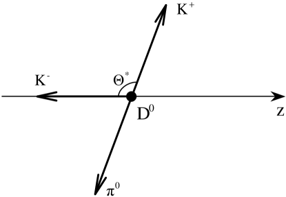
Figure 5: The $D^{0}\to K^{-}\,(K^{+}\pi^{0})_{K^{*+}}$ decay in the rest frame of $K^{+}$ and $\pi^{0}$.

$\cos\theta^{*}$ is given by

$$\cos\theta^{*}=\frac{m^{2}_{K^{-}\pi^{0}}-m^{2}_{K^{-}}-m^{2}_{\pi^{0}}-2E_{K^{-}}^{*}E_{\pi^{0}}^{*}}{2|{\bf p}_{K^{-}}^{*}||{\bf p}_{\pi^{0}}^{*}|}\ \ ,$$ (17)

so

$$A_{1}(m_{K^{+}\pi^{0}},\,m_{K^{-}\pi^{0}})\propto\frac{m^{2}_{K^{-}\pi^{0}}-m^{2}_{K^{-}}-m^{2}_{\pi^{0}}-2E_{K^{-}}^{*}E_{\pi^{0}}^{*}}{|{\bf p}_{K^{-}}^{*}|}\ \ ,$$ (18)

where

$$E_{K^{-}}^{*}=(m^{2}_{D^{0}}-m^{2}_{K^{-}}-m^{2}_{K^{+}\pi^{0}})/2m_{K^{+}\pi^{0}}\ \ ,$$ (19)

$$E_{\pi^{0}}^{*}=(m^{2}_{K^{+}\pi^{0}}-m^{2}_{K^{+}}+m^{2}_{\pi^{0}})/2m_{K^{+}\pi^{0}}\ \ ,$$ (20)

$$|{\bf p}_{K^{-}}^{*}|=\lambda^{1/2}(m^{2}_{D^{0}},m^{2}_{K^{-}},m^{2}_{K^{+}\pi^{0}})/2m_{K^{+}\pi^{0}}\ \ ,$$ (21)

$$|{\bf p}_{\pi^{0}}^{*}|=|{\bf p}_{K^{+}}^{*}|\ \ ,$$ (22)

$$\lambda(x,y,z)\equiv x^{2}+y^{2}+z^{2}-2xy-2xz-2yz\ \ .$$ (23)

Including the finite resonance width $\Gamma_{K^{*+}}$ into the $K^{*+}$ propagator, we can write the amplitude of the $D^{0}\to K^{-}\,(K^{+}\pi^{0})_{K^{*+}}$ decay as

$$A(D^{0}\to K^{-}\,(K^{+}\pi^{0})_{K^{*+}})\propto\frac{A_{1}(m_{K^{+}\pi^{0}},\,m_{K^{-}\pi^{0}})}{{m^{2}_{K^{+}\pi^{0}}-m^{2}_{K^{*+}}+i\,m_{K^{*+}}\Gamma}}\ \ .$$ (24)

As for the $D^{0}\to K^{+}\,(K^{-}\pi^{0})_{K^{*-}}$ decay, its amplitude can be derived in a similar way and is equal to

$$A(D^{0}\to K^{+}\,(K^{-}\pi^{0})_{K^{*-}})\propto r_{D}e^{i\delta_{D}}\,\frac{A_{2}(m_{K^{+}\pi^{0}},\,m_{K^{-}\pi^{0}})}{m^{2}_{K^{-}\pi^{0}}-m^{2}_{K^{*-}}+i\,m_{K^{*-}}\Gamma}\ \ ,$$ (25)

with the kinematic factor $A_{2}$ defined as $A_{2}(m_{K^{+}\pi^{0}},\,m_{K^{-}\pi^{0}})\equiv A_{1}(m_{K^{-}\pi^{0}},\,m_{K^{+}\pi^{0}})$. The factor $r_{D}e^{i\delta_{D}}$ accounts for possible differences in hadronization as vector particles between quarks arising from the virtual $W^{+}$ and spectator quarks.

Calculation of the fraction $\epsilon$ of resonant decays that fall into the square region

For the particular case of an on-shell resonant $K^{*+}$ we can neglect the Breit-Wigner denominator of Eq. (24). In this case the amplitude of the $D^{0}\to K^{-}\,(K^{+}\pi^{0})_{K^{*+}}$ decay is proportional to $A_{1}(m_{K^{*+}},\,m_{K^{-}\pi^{0}})$. The kinematics of the two-body $D^{0}\to K^{-}K^{*+}$ and $K^{*+}\to K^{+}\pi^{0}$ decays determine $E_{K^{-}}^{*}=1.37$ GeV, $E_{\pi^{0}}^{*}=0.32$ GeV, $|{\bf p}_{K^{-}}^{*}|=1.27$ GeV and $|{\bf p}_{\pi^{0}}^{*}|=0.29$ GeV. As a result, Eq. (17) says:

$$\cos\theta^{*}=1.36\,(m^{2}_{K^{-}\pi^{0}}-1.135)\ \ ,$$ (26)

where $m^{2}(K^{-}\pi^{0})$ is in GeV². Thus, the amplitude of the $D^{0}\to K^{-}\,(K^{+}\pi^{0})_{K^{*+}}$ decays is proportional to $(m^{2}_{K^{-}\pi^{0}}-1.135)$. These resonant decays fill the vertical band in a nonuniform way: no decays happen at the middle of the band where $m^{2}_{K^{-}\pi^{0}}-1.135=0$. The majority of the events will concentrate near both band ends where $|m^{2}_{K^{-}\pi^{0}}-1.135|$ is the largest.

Now we can calculate the fraction of $D^{0}\to K^{-}\,(K^{+}\pi^{0})_{K^{*+}}$ decays that fall into the square region,

$$\epsilon=\left.\int\limits_{0.75}^{0.84}(x-1.135)^{2}\,dx\right/\int\limits_{0.40}^{1.87}(x-1.135)^{2}\,dx=0.039\ \ ,$$ (27)

where $(m_{K^{*+}}-\Gamma/2)^{2}=0.75$ GeV² and $(m_{K^{*+}}+\Gamma/2)^{2}=0.84$ GeV² are the boundaries of the square region and $0.40$ and $1.87$ are the boundaries of the whole band. The latter can be derived from Eq. (26).

This simple calculation implied that the population density of the vertical band is constant along any cross section of the band, i.e., at a fixed $m^{2}_{K^{-}\pi^{0}}$ it is independent of variations of $m^{2}_{K^{+}\pi^{0}}$ across the band. A more precise discussion involves a simulation of the interference between the Breit-Wigner resonant shapes of Eqs. (24) and (25).

Appendix B: Influence of scalar resonance $\kappa$

The existence of broad scalar resonances below $1$ GeV has been a controversial issue for a long time [20]. A few experiments have been able to explore the possibility of their presence as intermediate resonant states in three-body $D$ decays. The modes that were studied include $D^{+}\to\pi^{-}\pi^{+}\pi^{+}$ [19], $D^{+}_{s}\to\pi^{-}\pi^{+}\pi^{+}$ [21], $D^{+}\to K^{-}\pi^{+}\pi^{+}$ [22]  (E791 collaboration), $D^{0}\to K^{0}_{S}\pi^{+}\pi^{-}$ [11], $D^{0}\to K^{-}\pi^{+}\pi^{0}$ [18]  (CLEO), and $D^{0}\to K^{0}K^{-}\pi^{+}$ [23]  (BaBar). The first two studies obtained evidence for a light ($478$ MeV) $\sigma$ resonance and measured the properties of the $f_{0}(980)$. The last four might provide some information on the presence of an intermediate S-wave $K\pi$ resonance. Indeed, the E791 analysis of a Dalitz plot found that the best fit to the data is obtained allowing for the presence of an additional scalar resonance $\kappa(800)^{0}$. However, neither CLEO studies found evidence for $\kappa^{0}$ or its isodoublet partner $\kappa^{+}$. The preliminary BaBar analysis saw $\kappa$ at the level of $1\sigma$ which does not allow the confirmation of its presence. Other types of decays could also provide a glimpse of $\kappa$. The BES collaboration found $\kappa^{0}$ as an intermediate state in $J/\psi\to\bar{K}^{*}(892)^{0}K^{+}\pi^{-}$ decays [24], while the FOCUS collaboration studied the interference phenomena in $D^{+}\to K^{-}\pi^{+}\mu^{+}\nu$ decays [25]. Their data can be described by $\bar{K}^{*0}$ interference with either a constant amplitude or a broad spin zero resonance.

The $D^{0}\to K^{\mp}K^{*\pm}$ decays discussed in this note can be affected by the possible presence of $\kappa^{\pm}$ among the intermediate states. The bands of a broad $\kappa(800)$ would cover more than 50% of the Dalitz plot, thereby interfering with the $K^{*}$ bands and affecting their population. One would expect that in this case the total branching ratio of $D^{0}\to K^{+}K^{-}\pi^{0}$ decays would be considerably larger than the sum of the $D^{0}\to KK^{*}$ modes. Indeed, in $D^{+}\to K^{-}\pi^{+}\pi^{+}$ an unusually high fraction (over 90%) of decays was found to be non-resonant by previous experiments [26]. That was unusual as the non-resonant (NR) contribution in three-body decays is small in most other cases. That was an indication of a possible broad scalar contribution and motivated the recent searches for it. It was found that the complex structure of the Dalitz plot was best explained when the $\kappa$ presence is assumed [22]. Then, intermediate decays through the $\kappa\pi^{+}$ state account for about 50% of decays while the NR fraction drops to a value of 13% more characteristic of other decays.

The present knowledge of $D^{0}\to K^{\mp}K^{*\pm}$ decays does not reveal a similar large non-resonant (or broad scalar) contribution. The current data on the resonant [15, 16] and inclusive [15, 27] decays comes from CLEO measurements. The inclusive branching ratio is ${\cal B}(D^{0}\to K^{+}K^{-}\pi^{0})=(1.24\pm 0.35)\cdot 10^{-3}$. The branching ratios of the $K\pi$ resonant decays are ${\cal B}(D^{0}\to K^{+}\,(K^{-}\pi^{0})_{K^{*-}})=\frac{1}{3}\,(2.0\pm 1.1)\cdot 10^{-3}=(0.67\pm 0.37)\cdot 10^{-3}$ and ${\cal B}(D^{0}\to K^{-}\,(K^{+}\pi^{0})_{K^{*+}})=\frac{1}{3}\,(3.8\pm 0.8)\cdot 10^{-3}=(1.27\pm 0.27)\cdot 10^{-3}$. Neglecting the interference between these two channels (it affects just about 4% of these decays; see Appendix A), the two branching ratios add up to $(1.93\pm 0.45)\cdot 10^{-3}$, consistent with the inclusive branching ratio within the current large uncertainties. Basically, there is no room for a broad scalar resonance channel. For example, it cannot negatively interfere with both halves of a $K^{*}$ band. The phase variation across it would be significant ($\approx 90^{\circ}$) for a $K^{*}$ channel and much smaller for a broad $\kappa$ one. If this channel is strong enough to cancel half the $K^{*}$ decays it would contribute many times more than that outside the $K^{*}$ bands. That would contradict the smallness of the inclusive branching ratio. Thus, we conclude that a broad scalar $\kappa$, if present, could only comprise a small fraction of $D^{0}\to K^{+}K^{-}\pi^{0}$ decays and would not significantly affect the estimate of the uncertainty in the strong phase $\delta_{D}$.

References

[1] M. Suzuki, Phys. Rev. D 58, 111504 (1998).
[2] J. L. Rosner, Phys. Rev. D 60, 074029 (1999).
[3] J. L. Rosner, Phys. Rev. D 60, 114026 (1999).
[4] C.-W. Chiang, Z. Luo, J. L. Rosner, Phys. Rev. D 67, 014001 (2003).
[5] A. F. Falk, Y. Nir, and A. A. Petrov, JHEP 9912, 019 (1999).
[6] S. Bergmann, Y. Grossman, Z. Ligeti, Y. Nir, and A. A.
Petrov, Phys. Lett. B 486, 418 (2000).
[7] H. J. Lipkin, Phys. Lett. B 494, 248 (2000).
[8] L. Wolfenstein, Phys. Rev. Lett. 75, 2460 (1995).
[9] Z. Z. Xing, Phys. Rev. D 53, 204 (1996); Phys. Lett. B 372, 317 (1996);
Phys. Lett. B 379, 257 (1996); Phys. Rev. D 55, 196 (1997); Phys. Lett. B 463, 323 (1999).
[10] M. Gronau, Y. Grossman, and J. L. Rosner, Phys. Lett. B 508, 37 (2001).
[11] CLEO Collaboration, H. Muramatsu et al., Phys. Rev. Lett. 89, 251802 (2002).
[12]
A. Palano [BABAR Collaboration], Proceedings of IX International Conference
on Hadron Spectroscopy (Hadron 2001), p. 53, Protvino, Russia, August 25 –
September 1, 2001, AIP Conference Proceedings. No. 619, p. 53 (2002).
[13] Y. Grossman, Z. Ligeti, and A. Soffer, Phys. Rev. D 67, 071301 (2003).
[14] The use of three-body decays has been proposed by
D. Atwood, I. Dunietz, and A. Soni, Phys. Rev. D 63, 036005 (2001)
and further developed by
A. Giri, Y. Grossman, A. Soffer, and J. Zupan,
hep-ph/0303187 (unpublished).
[15] Particle Data Group, K. Hagiwara et al.,
Phys. Rev. D 66, 010001 (2002).
[16] CLEO Collaboration, R. Ammar, Phys. Rev. D 44, 3383 (1991).
[17] CLEO Collaboration, R. A. Briere et al., “CLEO-c and CESR-c:
A New Frontier of Weak and Strong Interactions” (2001), CLNS-01-1742.
[18] CLEO Collaboration, S. Kopp et al., Phys. Rev. D 63, 092001 (2001).
[19] E791 Collaboration, E. M. Aitala et al., Phys. Rev. Lett. 86, 770 (2001).
[20]
E. van Beveren et al., Zeit. Phys. C 30, 615 (1986);
S. Ishida et al., Prog. Theor. Phys. 98, 621 (1997);
J. A. Oller, E. Oset and J. R. Pelaez,
Phys. Rev. D 59, 074001 (1999)
[Erratum-ibid. D 60, 099906 (1999)];
S. N. Cherry and M. R. Pennington, Nucl. Phys. A 688, 823 (2001);
F. E. Close and N. A. Tornqvist, J. Phys. G 28, R249 (2002);
P. Minkowski and W. Ochs, hep-ph/0209225.
[21] E791 Collaboration, E. M. Aitala et al., Phys. Rev. Lett. 86, 765 (2001).
[22] E791 Collaboration, E. M. Aitala et al., Phys. Rev. Lett. 89, 121801 (2002).
[23] BABAR Collaboration, B. Aubert et al., SLAC-PUB-9320, BABAR-CONF-02-031.
Contributed to 31st International Conference on High Energy Physics
(ICHEP 2002), Amsterdam, The Netherlands, 24-31 Jul 2002; hep-ex/0207089.
[24] BES Collaboration, J. Z. Bai et al., hep-ex/0304001.
[25] FOCUS Collaboration, J. M. Link et al., Phys. Lett. B 535, 43 (2002).
[26] E691 Collaboration, J. C. Anjos et al., Phys. Rev. D 48, 56 (1993);
E687 Collaboration, P. L. Frabetti et al., Phys. Lett. B 331, 217 (1994).
[27] CLEO Collaboration, D. M. Asner et al., Phys. Rev. D 54, 4211 (1996).