Abstract

In this paper $\gamma^{*}-\gamma^{*}$ scattering with large, but more or less equal virtualities of two photons is discussed using BFKL dynamics, emphasizing the large impact parameter behavior ($b_{t}$) of the dipole-dipole amplitude. It is shown that the non-perturbative contribution is essential to fulfill the unitarity constraints in the region of $b_{t}\,>\,1/2\,m_{\pi}$, where $m_{\pi}$ is pion mass. The saturation and the unitarization of the dipole-dipole amplitude is considered in the framework of the Glauber-Mueller approach. The main result is that we can satisfy the unitarity constraints introducing the non-perturbative corrections only in initial conditions ( Born amplitude).

1 Introduction.

In this paper we continue our investigation of $\gamma^{*}-\gamma^{*}$ scattering at high energies (see Ref.[1] for our previous attempts to study this process in the DGLAP dynamics). We concentrate our efforts here on the case of two photons with large but almost equal virtualities. It has been argued [2, 3] that this process is the perfect tool to recover the BFKL dynamics [4] which is the key problem in our understanding of the low $x$ ( high energy) asymptotic behavior in QCD.

It is well known that the correct degrees of freedom at high energy are not quarks or gluon but colour dipoles [5, 6, 7, 8] which have transverse sizes $r_{t}$ and the fraction of energy $z$. Therefore, two photon interactions occur in two successive steps. First, each virtual photon decays into a colour dipole ( quark - antiquark pair ) with size $r_{t}$. At large value of photon virtualities the probability of such a decay can be calculated in pQCD. The second stage is the interaction of colour dipoles with each other. The simple formula ( see for example Ref. [9] ) that describes the process of interaction of two photons with virtualities $Q_{1}$ and $Q_{2}$ ($\,\approx\,Q_{1}$ ) is (see Fig. 1 )

$$\sigma(Q_{1},Q_{2},W)\,\,=\,\,\int\,d^{2}b_{t}\sum^{N_{f}}_{a,b}\,\$$ (1.1)

$$\int^{1}_{0}\,d\,z_{1}\,\int\,d^{2}\,r_{1,t}|\Psi^{a}_{T,L}(Q_{1};z_{1},r_{1,t})|^{2}\,\,\int^{1}_{0}\,d\,z_{2}\,\int\,d^{2}\,r_{2,t}|\Psi^{b}_{T,L}(Q_{2};z_{2},r_{2,t})|^{2}\,\,2\,N(x,r_{1,t},r_{2,t};b_{t})$$

where the indexes $a$ and $b$ specify the flavors of interacting quarks, $T$ and $L$ indicate the polarization of the interacting photons where $r_{i}$ denote the transverse separation between quark and antiquark in the dipole ( dipole size) and $z_{i}$ are the energy fractions of the quark in the fluctuation of photon $i$ into quark-antiquark pair. $N(x,r_{1,t},r_{2,t};b_{t})$ is the imaginary part of the dipole - dipole amplitude at $x$ given by

$$x\,\,=\,\,\frac{Q^{2}_{1}\,+\,Q^{2}_{2}}{W^{2}\,+\,Q^{2}_{1}\,+\,Q^{2}_{2}}$$ (1.2)

for massless quarks ($W$ is the energy of colliding photons in c.m.f.). $b_{t}$ is the impact parameter for dipole-dipole interaction and it is equal the transverse distance between the dipole centers of mass.

The wave functions for virtual photon are known [10] and they are given by (for massless quarks)

$$|\Psi^{a}_{T}(Q;z,r_{t})|^{2} = \sum_{a}\,\frac{6\alpha_{em}}{\pi^{2}}\,Z^{2}_{a}\,\,(z^{2}\,+\,(1-z)^{2})\,\bar{Q}^{2}\,K^{2}_{1}(\bar{Q}\,r_{t})\,\,;$$ (1.3)

$$|\Psi^{a}_{L}(Q;z,r_{t})|^{2} = \sum_{a}\,\frac{6\alpha_{em}}{\pi^{2}}\,Z^{2}_{a}\,Q^{2}\,z^{2}\,(1-z)^{2}K^{2}_{0}(\bar{Q}\,r_{t})\,\,;$$ (1.4)

with $\bar{Q}^{2}_{a}\,\,=\,\,z(1-z)Q^{2}\,$ where $Z_{a}$ denote the faction of quark charge of flavor $a$.

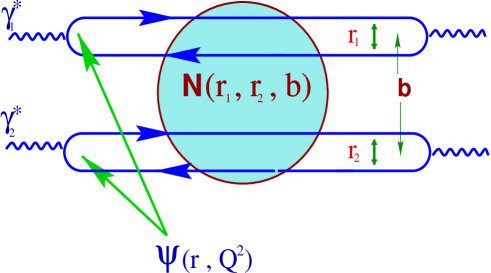
Figure 1: The picture of interaction of two photons with virtualities $Q_{1}$ and $Q_{2}$ larger than a “soft” scale.

Since the main contribution in Eq. (1.1) is concentrated at $r_{1,t}\,\approx\,1/Q_{1}\,\ll\,1/\mu$ and $r_{1,t}\,\approx\,1/Q_{2}\,\ll\,1/\mu$ where $\mu$ is the soft mass scale, we can safely use pQCD for calculation of the dipole-dipole amplitude $N$ in Eq. (1.1).

In this paper we study this process in the region of high energy and large but more-less equal photon virtualities ($Q^{2}_{1}\,\approx\,\,Q^{2}_{2}\,\,\gg\,\,1/\mu^{2}$) in the framework of the BFKL dynamics. In the region of very small $x$ (high energies) the saturation of the gluon density is expected [11, 12, 13]. We will deal with this phenomenon using Glauber-Mueller formula [5, 6, 7] which is the simplest one that reflects all qualitative features of a more general approach based on non-linear evolution [11, 12, 13, 14]. For $\gamma^{*}-\gamma^{*}$ scattering with large but equal photon virtualities, the Glauber-Mueller approach is the only one on the market since the non-linear equation is justified only for the case when one of the photon has larger virtuality than the other.

In the next section we discuss the dipole-dipole interaction in the BFKL approach of pQCD. The solution to the BFKL equation, that describes the dipole-dipole interaction in our kinematic region, has been found [15] and our main concern in this section is to find the large impact parameter ($b_{t}$) behavior of the solution. As was discussed in Ref. [16, 17, 18, 1], we have to introduce non-perturbative corrections in the region of $b_{t}$ larger than $1/2\,m_{\pi}$ where $m_{\pi}$ is the pion mass. We argue in this section that it is sufficient to introduce the non-perturbative behavior into the Born approximation to obtain a reasonable solution at large $b_{t}$.

Section 3 is devoted to Glauber - Mueller formula in the case of the BFKL emission [4]. Here, we use the advantage of photon - photon scattering with large photon virtualities, since we can calculate the gluon density without uncertainties related to non-perturbative initial distributions in hadronic target. We consider the low $x$ behavior of the dipole-dipole cross section and show that the large impact parameter behavior, introduced in the Born cross section, fulfills the unitarity restrictions ( unitarity bound [19]). Therefore, we confirm that the large $b_{t}$ behavior can be concentrated in the initial condition (see Refs. [16, 18, 1] without changing the kernel of the non-linear equation that governs evolution in the saturation region as it is advocated in Ref.[17].

In the last section we summarize our results.

2 Dipole-dipole interaction in the BFKL approximation.

In this section we discuss the one parton shower interaction in the BFKL dynamics ( see Fig. 3). We start with the Born approximation which is the exchange of two gluons (see Fig. 2 ) or the diagrams of Fig. 3 without emission of a gluon.

2.1 Born Approximation:   

These diagrams have been calculated in Ref. [1] using the approach of Ref. [20] and they lead to the following expression for the dipole-dipole amplitude:

$$N^{BA}(r_{1,t},r_{2,t};b_{t})\,\, = \,\,\,\pi\alpha_{S}^{2}\frac{N^{2}_{c}-1}{2\,N^{2}_{c}}\,\,\left(\,\ln\frac{(\vec{b}\,-\,z_{1}\vec{r}_{1}\,-\,z_{2}\vec{r}_{2})^{2}\,\,(\vec{b}\,-\,\bar{z}_{1}\vec{r}_{1}\,-\,\bar{z}_{2}\vec{r}_{2})^{2}}{(\vec{b}\,-\,\bar{z}_{1}\vec{r}_{1}\,-\,z_{2}\vec{r}_{2})^{2}\,\,(\vec{b}\,-\,z_{1}\vec{r}_{1}\,-\,\bar{z}_{2}\vec{r}_{2})^{2}}\,\right)^{2}$$ (2.5)

$$= \,\,\pi\alpha_{S}^{2}\frac{N^{2}_{c}-1}{2\,N^{2}_{c}}\,\ln^{2}\left(\frac{\rho^{2}_{1,1^{\prime}}\,\rho^{2}_{2,2^{\prime}}}{\rho^{2}_{1,2^{\prime}}\,\rho^{2}_{2,1^{\prime}}}\right)$$ (2.6)

where $z_{i}$ is the fraction of the energy of the dipole carried by quarks; $\bar{z}_{i}\,=\,z_{i}\,-\,1$ and $\rho_{i,k}\,=\,\vec{\rho}_{i}-\vec{\rho}_{k}$. $\vec{\rho}_{i}$ is the coordinate of quark $i$ (see Fig. 2). All vectors are two dimensional in Eq. (2.5).

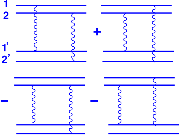
Figure 2: Dipole-dipole interaction in the Born approximation.

Each diagrams in Fig. 2 is easy to calculate [24] and the first diagram is equal to

$$\pi\alpha_{S}^{2}\frac{N^{2}_{c}-1}{2\,N^{2}_{c}}\,\ln\rho^{2}_{1,1^{\prime}}\,\,\ln\rho^{2}_{2,2^{\prime}}\,\,.$$ (2.7)

Summing all diagrams we obtain Eq. (2.5).

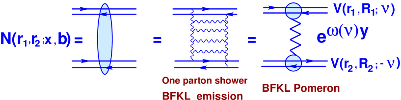
Figure 3: One parton shower interaction in the BFKL approach.

We are interested mostly in the limit of large $b_{t}\,\,\gg\,\,r_{1,t}\,\approx\,\,r_{2,t}$ where the dipole-dipole amplitude can be reduced to a simple form.

$$N^{BA}(r_{1,t},r_{2,t};b_{t})\,\,\rightarrow\,\,\pi\alpha_{S}^{2}\frac{N^{2}_{c}-1}{N^{2}_{c}}\,\,\frac{r^{2}_{1,t}\,\,r^{2}_{2,t}}{b^{4}_{t}}\,\,,$$ (2.8)

after integration over azimuthal angles.

Therefore, we have a power-like decrease of the dipole-dipole amplitude at large $b_{t}$ , namely $N^{BA}\,\propto\,\frac{r^{2}_{1,t}\,\,r^{2}_{2,t}}{b^{4}_{t}}$. Such behavior cannot be correct since it contradicts the general postulates of analyticity and crossing symmetry of the scattering amplitude [19]. Since the spectrum of hadrons has no particles with mass zero, the scattering amplitude should decrease as $e^{-2m_{\pi}\,b_{t}}$ [19]. In Ref. [1] we suggested a procedure of how to cure this problem which is based on the results of QCD sum rules [21].Following this procedure we rewrite the dipole-dipole amplitude as the integral over the mass of two gluons in $t$-channel; and we assume, as in QCD sum rules, that this integral describes all hadronic states on average. Restricting the integral over mass by the minimal mass of hadronic states ( 2 $m_{\pi}$ ) we obtain the model which provides the exponential fall at large $b_{t}\,\gg\,1/(2\,m_{\pi})$ and does not change the power like behavior for small $b_{t}\,\ll\,1/(2\,m_{\pi})$.

We choose for the Born amplitude the following formula

$$N^{BA}(r_{1,t},r_{2,t};b_{t})\,\,=\,\,\pi\alpha_{S}^{2}\frac{N^{2}_{c}-1}{N^{2}_{c}}\,\,\frac{r^{2}_{1,t}\,r^{2}_{1,t}\,m^{4}_{\pi}}{3}\,K_{4}(2\,m_{\pi}b_{t})\,\,.$$ (2.9)

One can easily see that Eq. (2.9) reproduces Eq. (2.8) and leads to

$$N^{BA}(r_{1,t},r_{2,t};b_{t})\,\,\rightarrow\,\,\pi\alpha_{S}^{2}\frac{N^{2}_{c}-1}{N^{2}_{c}}\,\,\frac{r^{2}_{1,t}\,r^{2}_{2,t}\,m^{4}_{\pi}}{3}\,\sqrt{\frac{\pi}{2\,m_{\pi}\,b_{t}}}\,e^{-2\,m_{\pi}\,b_{t}}\,\,.$$ (2.10)

at large $b_{t}\,\,\gg\,\,1/(2\,m_{\pi})$.

2.2 BFKL equation:

The emission of a gluon is described by the BFKL equation [4] which was solved in Ref.[15] for fixed $b_{t}$ (see Ref.[22, 23, 24] for many useful discussion of the different aspects of the solution). The solution can be presented in factorized form (see Fig. 3 ).

$$N(x,r_{1,t},r_{2,t};b_{t})\,\,=$$ (2.11)

$$\int\frac{d\nu}{2\,\pi\,i}\,\phi_{in}(\nu;r_{1,t};b_{t})\,\,d^{2}\,R_{1}\,\,d^{2}\,R_{2}\,\delta(\vec{R}_{1}-\vec{R}_{2}-\vec{b}_{t})\,e^{\omega(\nu)\,y}\,V(r_{1,t},R_{1};\nu)\,V(r_{2,t},R_{2};-\nu)$$

with

$$\omega(\nu)\,\,=\,\,\frac{\alpha_{S}N_{c}}{\pi}\,\left(\,2\,\psi(1)\,-\,\psi(\frac{1}{2}-i\,\nu)\,-\,\psi(\frac{1}{2}+i\,\nu)\,\right)\,;$$ (2.12)

where $\psi(f)\,=\,d\ln\Gamma(f)/df$,$\Gamma(f)$ is Euler gamma function and where

$$V(r_{i,t},R_{i};\nu)\,\,=\,\,\left(\,\frac{r^{2}_{i,t}}{(\vec{R}_{i}\,+\,\frac{1}{2}\vec{r}_{i,t})^{2}\,\,(\vec{R}_{i}\,-\,\frac{1}{2}\vec{r}_{i,t})^{2}}\,\right)^{\frac{1}{2}\,-\,i\,\nu}$$ (2.13)

using the following notations: $y\,=\,\ln(x_{0}/x)$;  $r_{i.t}$ is the size of the colour dipole $``i"$ and $R_{i}$ is the position of the center of mass of this dipole. In Eq. (2.11) function $\phi_{in}(\nu;r_{2,t};b_{t})$ should be found from the initial condition which determines the dipole amplitude at fixed $x=x_{0}$, namely, $N(x=x_{0},r_{1,t},r_{2,t};b_{t})\,\,=\,\,N^{BA}(x=x_{0},r_{1,t},r_{2,t};b_{t})$.

It should be stressed that the BFKL equation is a linear equation in which the kernel does not depend on $b_{t}$ (see Ref.[14]). Therefore, $\phi_{in}(\nu;b_{t})$ could be an arbitrary function on $b_{t}$.

In Eq. (2.11) we can take the integral over $R_{2}$ which leads to

$$V(r_{2,t},R_{2};-\nu)\,\,=\,\,\left(\,\frac{r^{2}_{2,t}}{(\vec{R}_{1}\,+\,\vec{b}_{t}\,+\,\frac{1}{2}\vec{r}_{2,t})^{2}\,\,(\vec{R}_{1}\,+\,\vec{b}_{t}\,-\,\frac{1}{2}\vec{r}_{2,t})^{2}}\,\right)^{\frac{1}{2}\,+\,i\,\nu}\,\,.$$ (2.14)

We are interested in the large $b_{t}$ behavior, namely, $b_{t}\,\,\gg\,\,r_{1,t}\,\approx\,\,r_{2,t}$. It is instructive to consider two cases:

• DLA: ${\frac{1}{2}-i\,\nu\,\,\rightarrow\,\,0}$. This is so called double log approximation of pQCD (DLA) in which we consider $r_{1,t}\,\ll\,r_{2,t}$ and $\alpha_{S}\ln(1/x)\,\ln(r^{2}_{2,t}/r^{2}_{1,t})\,\,\approx\,1$ while $\alpha_{S}\ln(1/x)\,\ll\,1$ as well as $\alpha_{S}\ln(r^{2}_{2,t}/r^{2}_{1,t})\,\ll\,1$ and $\alpha_{S}\,\ll\,1$. We have considered this case in Ref.[1] and found that the emission of gluons does not induce any additional dependence on $b_{t}$ which is concentrated only in the Born amplitude. Indeed, we can see this property directly from the solution of Eq. (2.11).

  Integrating over $R_{1}$ we find that the integrand of this integral falls down rapidly for $R_{1}\,>\,b_{t}$ due to $R_{1}$ dependence of the vertex $V(r_{2,t},R_{2};\nu)$ (see Eq. (2.14)) providing a good convergence for the integral. For $R_{1}<b_{t}$ we can neglect $R_{1}$ dependence of the vertex $V(r_{2,t},R_{2};\nu)$ and consider it as $\left(\frac{r^{2}_{2,t}}{b^{4}_{t}}\right)^{\frac{1}{2}+i\,\nu}$ . The integral over $R_{1}$ of $V(r_{1,t},R_{1},\nu)$ for $R_{1}<b_{t}$ gives $\,(r_{1,t})^{\frac{1}{2}-i\,\nu}\,(b^{2}_{t})^{2\,i\,\nu}\,$.

  Therefore, $\int d^{2}R_{1}V(r_{1,t},R_{1},\nu)\,\,V(r_{2,t},b_{t},\nu)\,\,\rightarrow\,\,(r^{2}_{2,t}/b^{2}_{t})\,(r^{2}_{1,t}/r^{2}_{2})^{\frac{1}{2}-i\,\nu}$. Finally, taking $\phi_{in}(\nu;r_{1,t};b_{t})\,=\,\pi\,\alpha_{S}\,\frac{N^{2}_{c}-1}{3\,\,N^{2}_{c}}\,\,(m_{\pi}\,)^{2}\,(r_{1,t}\,b_{t})^{2}\,\,K_{4}(2\,m_{\pi}\,b_{t})\,\frac{1}{\ \frac{1}{2}\,-\,i\,\nu}\,\,$, the dipole amplitude has a form

  $$N^{DLA}(x,r_{1,t},r_{2,t};b_{t})\,=\,N^{BA}(x,r_{1,t},r_{2,t};b_{t})\,\int\,\frac{d\nu}{2\,\pi\,i}\,\,e^{\omega(\nu)\,y\,\,+\,\,(\frac{1}{2}\,-\,i\,\nu)\,\ln(r^{2}_{1,t}/r^{2}_{2,t})}$$ (2.15)

  Considering $r_{2,t}\,\ll\,r_{1,t}$ and taking into account that $\omega(\nu)\,\,\rightarrow\frac{\alpha_{S}N_{c}}{\pi}\,\frac{1}{\frac{1}{2}\,-\,i\,\nu}$ at $\frac{1}{2}\,-\,i\,\nu\,\rightarrow\,0$ one can take the integral in Eq. (2.15) explicitly. The answer is well known ( see Ref.[1] for example), namely, at low $x$

  $$N^{DLA}(x,r_{1,t},r_{2,t};b_{t})\,\,=\,\,N^{BA}(x,r_{1,t},r_{2,t};b_{t})\,\,I_{0}\left(2\sqrt{\frac{\alpha_{S}\,N_{c}}{\pi}\,y\,\ln(r^{2}_{2,t}/r^{2}_{1,t})}\,\right)$$ (2.16)

  for fixed coupling constant.

• Diffusion approximation: ${\nu\,\,\ll\,\,1}$. For such small values of $\nu$ the integral over $R_{1}$ is convergent for $R_{1}\,>r_{1,t}$ (see Ref.[22] ) and, therefore, we neglect the $R_{1}$ dependence in $V(r_{2,t},b_{t},\nu)$. Introducing a new variable $\vec{\xi}=\vec{R}_{1}/r_{1,t}$ we see that

  $$\int d^{2}\,R_{1}V(r_{1,t},R_{1};\nu)\,=\,(r^{2}_{1,t})^{\frac{1}{2}+i\,\nu}\,\int d^{2}\xi\left(\vec{\xi}+\frac{1}{2}\,\vec{n})^{2}\,(\vec{\xi}-\frac{1}{2}\,\vec{n})^{2}\,\right)^{\frac{1}{2}+i\,\nu}$$ (2.17)

  where $\vec{n}$ is a unit vector in the direction of $\vec{r}_{1,t}$. The integral is a function of $\nu$ only and can be absorbed in $\phi_{in}(\nu;b_{t})$ in Eq. (2.11). For $V(r_{2,t},b_{t},-\nu)$ at $b_{t}\,\gg\,r_{2,t}$ we have

  $$V(r_{2,t},b_{t},-\nu)\,\,=\,\,\left(\frac{r^{2}_{2,t}}{b^{4}_{t}}\right)^{\frac{1}{2}+i\,\nu}$$ (2.18)

  Therefore, the dipole amplitude is

  $$N^{DF}(x,r_{1,t},r_{2,t};b_{t})\,\,=\,\,\int\,\frac{d\nu}{2\,\pi\,i}\,\phi_{in}(\nu;b_{t})\,\,e^{\omega(\nu)\,y}\,\,\left(\,\frac{r^{2}_{1,t}\,r^{2}_{2,t}}{b^{4}_{t}}\,\right)^{\frac{1}{2}+i\,\nu}\,\,.$$ (2.19)

  We choose $\phi_{in}(\nu;b_{t})$ to be of in the form

  $$\phi_{in}(\nu;b_{t})\,\,=\,\,\pi\,\alpha_{S}\,\frac{N^{2}_{c}-1}{3\,\,N^{2}_{c}}\,\,(m_{\pi}\,b_{t})^{4}\,\,K_{4}(2\,m_{\pi}\,b_{t})\,\frac{1}{\ \frac{1}{2}\,-\,i\,\nu}\,\,.$$ (2.20)

  At small values of $\nu$ we can expand $\omega(\nu)$

  $$\omega(\nu)\,\,=\,\,\omega_{L}\,\,-\,\,D\,\nu^{2}$$ (2.21)

  with

  $$\omega_{L}\,\,=\,\,\frac{\alpha_{S}\,N_{c}}{\pi}\,4\,\ln 2\,\,;\,\,\,\,\,\,\,\,\,\,\,D\,\,=\,\,\frac{\alpha_{S}\,N_{c}}{\pi}\,\,14\,\zeta(3)\,\,;$$ (2.22)

  Finally, we can evaluate the integral over $\nu$ in Eq. (2.19) using the method of steepest decent and obtain the following expression for dipole amplitude:

  $$N^{DF}(x,r_{1,t},r_{2,t};b_{t})\,\,=$$ (2.23)

  $$\pi\,\alpha_{S}\,\frac{2(N^{2}_{c}-1)}{3\,\,N^{2}_{c}}\,\,(\,r_{1,t}\,r_{2,t}\,m^{4}_{\pi}\,b^{2}_{t}\,)\,K_{4}(2\,m_{\pi}\,b_{t})\,\,\sqrt{\frac{\pi}{D\,y}}\,\,e^{\omega_{L}\,y\,\,-\,\,\frac{\ln^{2}\frac{r^{2}_{1,t}\,r^{2}_{2,t}}{b^{4}_{t}}}{4\,D\,y}}$$

  At $1/(2\,m_{\pi})>\,b_{t}\,>\,r_{1,t}\,\approx\,r_{2,t}$

  $$N^{DF}(x,r_{1,t},r_{2,t};b_{t})\,\,\rightarrow$$ (2.24)

  $$\pi\,\alpha_{S}\,\frac{2(N^{2}_{c}-1)}{3\,N^{2}_{c}}\,\,\frac{r_{1,t}\,r_{2,t}}{b^{2}_{t}}\,\sqrt{\frac{\pi}{D\,y}}\,\,e^{\omega_{L}\,y\,\,-\,\,\frac{\ln^{2}\frac{r^{2}_{1,t}\,r^{2}_{2,t}}{b^{4}_{t}}}{4\,D\,y}}$$

  while at $b_{t}\,>\,1/(2\,m_{\pi})$

  $$N^{DF}(x,r_{1,t},r_{2,t};b_{t})\,\,\rightarrow$$ (2.25)

  $$\pi\,\alpha_{S}\,\frac{2(N^{2}_{c}-1)}{3\,N^{2}_{c}}\,\,(\,r_{1,t}\,r_{2,t}\,m^{4}_{\pi}\,b^{2}_{t}\,)\,\sqrt{\frac{\pi}{2\,m_{\pi}\,b_{t}}}\sqrt{\frac{\pi}{D\,y}}\,\,e^{\omega_{L}\,y\,\,-\,\,\frac{\ln^{2}\frac{r^{2}_{1,t}\,r^{2}_{2,t}}{b^{4}_{t}}}{4\,D\,y}\,\,-\,\,2\,m_{\pi}\,b_{t}}\,\,\,$$

3 Saturation and unitarization in the Glauber - Mueller approach.

3.1 Glauber - Mueller formula.

The Glauber - Mueller approach [5, 6, 7] takes into account the interaction of many parton showers with the target as is shown in Fig. 4. In our case of more or less equal but large virtualities of both photons this approach gives a unique opportunity to study the high energy asymptotic behavior of the dipole amplitude since other methods based on non-linear evolution equation [11, 12, 13, 14, 25, 26] do not work in the case of two dipoles with more-less equal sizes.

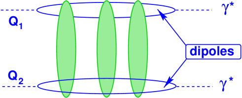
Figure 4: The Glauber - Mueller approach for the dipole-dipole scattering amplitude.

The main idea of this approach is that the colour dipoles are the correct degrees of freedom for high energy scattering (this idea was formulated by A.H. Mueller in Ref. [8]). Indeed, the change of the value of the dipole size $r_{t}$ ($\Delta r_{t}$) during the passage of the colour dipole through the target is proportional to the number of rescatterings (or the size of the target $R$) multiplied by the angle $k_{t}/E$ where $E$ is the energy of the dipole and $k_{t}$ is the transverse momentum of the $t$-channel gluon which is emitted by the fast dipole.

$$\Delta\,r_{t}\,\,\propto\,\,R\,\frac{k_{t}}{E}\,\,.$$ (3.26)

Since $k_{t}$ and $r_{t}$ are conjugate variables and due to the uncertainty principle

$$k_{t}\,\,\propto\,\,\frac{1}{r_{t}}\,\,.$$

Therefore,

$$\Delta\,r_{t}\,\,\propto\,\,R\,\frac{k_{t}}{E}\,\,\ll\,\,r_{t}\,\,\,\mbox{if}\,\,\,\,R\,\ll\,\,r^{2}_{t}\,\,E\,\,\,\mbox{or}\,\,\,x\,\,\ll\,\,\frac{1}{2m\,R}\,\,.$$ (3.27)

Since the colour dipoles are correct degrees of freedom , they diagonalize the interaction matrix at high energy as well as the unitarity constraints, which have the form

$$2\,\,N(x,r_{1,t},r_{2,t};b_{t})\,\,=\,\,|a_{el}(x,r_{1,t},r_{2,t};b_{t})|^{2}\,\,+\,\,G_{in}(x,r_{1,t},r_{2,t};b_{t})\,\,,$$ (3.28)

where $a_{el}$ is the elastic amplitude of the dipole-dipole interaction and $N$ is the imaginary part of $a_{el}$ ($N=Im\,a_{el}$).

Assuming that the amplitude is pure imaginary at high energy, one can find a simple solution to Eq. (3.28), namely

$$a_{el}(x,r_{1,t},r_{2,t};b_{t})\,\, = \,\,i\,\left(1\,\,-\,\,e^{-\frac{\Omega(x,r_{1,t},r_{2,t};b_{t})}{2}}\,\right)\,\,;$$ (3.29)

$$G_{in}(x,r_{1,t},r_{2,t};b_{t})\,\, = \,\,\left(1\,\,-\,\,e^{-\Omega(x,r_{1,t},r_{2,t};b_{t})}\,\right)\,\,;$$ (3.30)

where $\Omega$ is the arbitrary real function.

In Glauber - Mueller approach the opacity $\Omega$ is chosen as $\Omega=2\,N^{OPS}(x,r_{1,t},r_{2,t};b_{t})$ where $N^{OPS}$ is the dipole-dipole amplitude for one parton shower interaction that has been found in the previous section (see Eq. (2.11)).

3.2 Saturation.

One can see that if we substitute the explicit solution to the BFKL equation of Eq. (2.23) at any fixed $b_{t}$ the opacity $\Omega=2N^{DF}$ increases at $x\,\rightarrow\,0$. Therefore, the dipole-dipole amplitude given by Glauber-Mueller formula of Eq. (3.29) tends to unity in the region of low $x$. This statement is called saturation [11, 12, 13] since the physical interpretation of $N$ is the density of colour dipoles at least when $N$ is not very large. In this discussion the saturation appears to be the consequence of unitarity for fixed $b_{t}$. However, we have learned several examples where the dipole density could reach a maximum value without having any effect on the elastic dipole-dipole amplitude at fixed $b_{t}$ (see Ref. [13] and paper of Kovchegov and Mueller in Ref.[25]). However, for $\gamma^{*}-\gamma^{*}$ scattering of two small dipoles the initial condition is given by Born amplitude of Eq. (2.5) which is small. Therefore, we have no reason to expect that the dipole density will be high due to the final state interaction.

3.3 Unitarization.

To obtain the unitarity bound for the dipole-dipole cross section we have to integrate over $b_{t}$, namely

$$\sigma(dipole-dipole)\,=\,2\int d^{2}\,b_{t}\,N^{GM}(x,r_{1,t},r_{2,t};b_{t})=2\int d^{2}\,b_{t}\,\left(1\,-\,e^{-N^{DF}(x,r_{1,t},r_{2,t};b_{t})}\right)$$ (3.31)

Following Froissart [19], we divide the region of integration over $b_{t}$ in Eq. (3.31) in two parts

$$\sigma(dipole-dipole)\,\,=\,\,2\pi\int^{b^{2}_{0}(x)}_{0}\,d\,b^{2}_{t}\,\,N^{GM}(...;b_{t})\,\,+\,\,\int^{\infty}_{b^{2}_{0}(x)}\,db^{2}_{t}\,\,N^{GM}(...;b_{t})$$ (3.32)

where $b_{0}(x)$ is defined from the equation

$$N^{DF}(x,r_{1,t},r_{2,t};b_{0}(x))=1\,\,\,$$ (3.33)

It is easy to see that for $b_{t}\,<\,b_{0}(x)$ $N^{GM}\,\leq\,1$ since $N^{DF}\,>\,1$, while for $b_{t}\,\,\geq\,\,1$ and for $N^{DF}\,<\,1$   $N^{GM}\,\leq\,N^{DF}$ Therefore, we have the following unitarity bound

$$\sigma(dipole-dipole)\,\,\leq\,\,2\,\pi\,\left(\,b^{2}_{0}(x)\,\,+\,\,\int^{\infty}_{b_{0}(x)}\,db^{2}_{t}\,N^{GM}(...;b_{t})\,\right)$$ (3.34)

Let us consider two possibilities. The first one that $b_{0}(x)\,\,\ll\,1/(2\,m_{\pi})$. In this case the solution to Eq. (3.33) follows directly from Eq. (2.24) for the amplitude $N^{DF}$ and for $y\,\gg\,1$

$$\ln(\frac{r^{2}_{1,t}\,r^{2}_{2,t}}{b^{4}_{0}(x)})\,\,=\,\,-2\,\sqrt{\,D\,\omega_{L}}\,y$$ (3.35)

or

$$b^{2}_{0}(x)\,\,\propto\,\,r_{1,t}\,r_{2,t}\,\,e^{\sqrt{\,D\,\omega_{L}}\,y}$$ (3.36)

Substituting Eq. (3.36) into Eq. (3.34) we can obtain

$$\sigma(dipole-dipole)\,\,\leq\,\,2\,\pi\,b^{2}_{0}(x)\,\{\,1\,+\,2\,\}\,\,\propto\,\,e^{\sqrt{\frac{\,D\,\omega_{L}}{2}}\,y}$$ (3.37)

where the second term is calculated by integrating first over $b_{t}$ Eq. (2.19) and after that using saddle point approach. Since $\nu_{SADDLE}$ turns out to be small at low $x$ and we neglect it.

Therefore, in this kinematic region we face a power -like increase of the dipole-dipole cross section as was pointed out in Refs. [17].

However, this power-like increase will stop for $b_{0}(x)\,>\,1/2\,m_{\pi}$. Indeed, for such large values of $b_{t}$ we should use Eq. (2.25) for the dipole amplitude $N^{DF}$. For such large values of $b_{0}(x)$ Eq. (3.33) has a solution which at low $x$ is

$$b_{0}(x)\,\,=\,\,\frac{\omega_{L}}{2m_{\pi}}\,y\,\,+\,\,O(lny)$$ (3.38)

which leads to

$$\sigma(dipole-dipole)\,\,\leq\,\,2\,\pi\,b^{2}_{0}(x)\,\,=\,\,\frac{2\pi\,\omega_{L}^{2}}{4\,m^{2}_{\pi}}\,\ln^{2}(x_{0}/x)$$ (3.39)

which comes from the first term in Eq. (3.34). It is easy to understand that the second term in this equation gives a term which does not increase with $y$. Eq. (3.39) is the unitarity bound which has the same energy dependence as for hadron-hadron collisions [19] but in our approach we are able to calculate the coefficient in front of $y^{2}$. The bound of Eq. (3.39) is the same as was derived in [16, 18].

It should be stressed that the diffusion approximation that we used was derived only at small values of saddle point in $\nu$ integration in Eq. (2.19) which is equal to

$$|\nu_{SADDLE}|\,\,=\,\,\frac{\ln\frac{r^{2}_{1,t}\,r^{2}_{2,t}}{b^{4}_{0}(x)}}{2\,D\,y}\,\,\ll\,\,1$$ (3.40)

at $b_{t}=b_{0}(x)$ from Eq. (3.38).

3.4 Saturation scale.

Eq. (3.33) does not have a solution at any values of $r_{1,t}$ and $r_{2,t}$ (formally, we obtain a negative values of $b_{0}(x)$). The same equation at $b_{t}=0$, namely

$$N(x,r_{sat},r_{2,t};b_{t}=0)\,\,=\,\,1\,\,,$$ (3.41)

determines the saturation scale. At $r_{1,t}\,\geq\,r_{sat}$ the opacity $\Omega$ in Glauber-Mueller formula is larger than unity ($\Omega\,\geq\,1$), Eq. (3.33) has a solution and we are in the saturation region with Eq. (3.39) for the unitarity bound. If $r_{1,t}\,\leq\,r_{sat}$, opacity $\Omega\,<\,1$ at any value of $b_{t}$. This is a domain of perturbative QCD in virtual photon scattering.

$N(x,r_{1,t},r_{2,t};b_{t}=0)$ we can find from Eq. (2.11) integrating over $R_{1}$, namely

$$N(x,r_{1,t},r_{2,t};b_{t}=0)\,\,=\int\frac{d\nu}{2\,\pi\,i}\,\phi_{in}(\nu;b_{t}=0)\,\,d^{2}\,R_{1}\,\,e^{\omega(\nu)y}\,V(r_{1,t},R_{1};\nu)\,V(r_{2,t},R_{1};-\nu)\,\,.$$ (3.42)

Since $r_{sat}$ from Eq. (3.41) is much smaller than $r_{2,t}$ we need to find Eq. (3.42) only for $r_{1,t}\,\ll\,r_{2,t}$. This observation simplifies the calculations. Indeed, the main contribution in the integral over $R_{1}$ stems from $R_{1}\ll r_{2,t}$. Therefore, we can neglect the $R_{1}$ - dependence of vertex $V(r_{2,t},R_{1};-\nu)$ which has the form

$$V(r_{2,t},R_{1};-\nu)\,\,=\,\,\left(\frac{16}{r^{2}_{2,t}}\right)^{\frac{1}{2}+i\,\nu}\,\,.$$ (3.43)

To perform the integration over $R_{1}$ we use the following formula ( see equation 3.198 of Ref.[27] )

$$B(\frac{1}{2}-i\nu,\frac{1}{2}-i\nu)\,\left(\,\frac{1}{(\vec{R}_{i}\,+\,\frac{1}{2}\vec{r}_{i,t})^{2}\,\,(\vec{R}_{i}\,-\,\frac{1}{2}\vec{r}_{i,t})^{2}}\,\right)^{\frac{1}{2}\,-\,i\,\nu}\,\,=$$ (3.44)

$$\,\,\int^{1}_{0}\,d\,t\,\,(\,t(1-t)\,)^{-\frac{1}{2}-i\,\nu}\left(\,R^{2}_{1}\,+\,(1-2t)\vec{R}_{1}\,\cdot\,\vec{r}_{1,t}\,+\,\frac{r^{2}_{1,t}}{4}\,\right)^{-1+2i\,\nu}\,\,,$$

where $B(\mu,\nu)=\Gamma(\mu)\Gamma(\nu)/\Gamma(\mu+\nu)$ is the Euler beta - function. Integrating Eq. (3.42) over $R_{1}$ using Eq. (3.44) we obtain that

$$N(x,r_{1,t},r_{2,t};b_{t}=0)\,\,=\int\frac{d\nu}{2\,\pi\,i}\,\phi_{in}(\nu;b_{t})\,\,e^{\omega(\nu)y}\,\frac{B(\frac{1}{2}+i\nu,\frac{1}{2}+i\nu)}{B(\frac{1}{2}-i\nu,\frac{1}{2}-i\nu)}\,\,\frac{1}{2\,i\,\nu}\left(\frac{16\,r^{2}_{1,t}}{r^{2}_{2,t}}\right)^{\frac{1}{2}+\,i\,nu}$$ (3.45)

The Born approximation at $b_{t}=0$ and at $r_{2,t}\,\,\geq\,r_{1,t}$ can be reduced to [1]

$$N^{BA}(r_{1,t},r_{2,t};b_{t}=0)\,\,\rightarrow\,\,\pi\alpha_{S}^{2}\,\frac{N^{2}_{c}-1}{N^{2}_{c}}\,\,\frac{r^{2}_{1,t}}{z^{2}_{2}\,\tilde{z}^{2}_{2}\,\,r^{2}_{2,t}}\,\,.$$ (3.46)

It is easy to choose $\phi_{in}(\nu;b_{t}=0)$ in such a way that the final answer for $N(x,r_{1,t},r_{2,t};b_{t}=0$ is:

$$N(x,r_{1,t},r_{2,t};b_{t}=0)\,\,=\pi\alpha_{S}^{2}\,\frac{N^{2}_{c}-1}{N^{2}_{c}\,z^{2}_{2}\,\tilde{z}^{2}_{2}}\int\frac{d\nu}{2\,\pi\,i}\,\frac{1}{\frac{1}{2}-i\nu}\,,e^{\omega(\nu)y\,\,+\,\,(\frac{1}{2}+i\nu)\,\ln(r^{2}_{1,t}/r^{2}_{2,t})}\,\,.$$ (3.47)

We can find the solution to Eq. (3.41) in the saddle point approximation for the integral over $\nu$ in Eq. (3.47) [11, 28]. Introducing a new variable $\gamma=\frac{1}{2}+i\nu$ we have the following equation for the saddle point value of $\gamma=\gamma_{S}$:

$$\frac{d\omega(\gamma)}{d\gamma}|_{\gamma=\gamma_{S}}\,y+\,ln(r^{2}_{1,t}/r^{2}_{2,t})\,\,=0$$ (3.48)

Substituting Eq. (3.48) in Eq. (3.47) we obtain

$$N(x,r_{1,t},r_{2,t};b_{t}=0)\,\,\propto\,\,e^{\omega(\gamma_{S})\,y\,-\gamma_{S}\ln(r^{2}_{2,t}/r^{1}_{2,t})}\,\,=\,\,e^{y\,\{\omega(\gamma_{S})\,\,-\,\,\gamma_{S}\,\frac{d\omega(\gamma)}{d\gamma}|_{\gamma=\gamma_{S}}\}}$$ (3.49)

Using Eq. (3.49) we can solve Eq. (3.41) in semiclassical approximation ( see Ref. [11, 25] in which we cannot calculate the numerical factor in front of Eq. (3.49) . Indeed, $N(x,r_{1,t},r_{2,t};b_{t}=0)$ is constant on the line

$$\frac{d\omega(\gamma)}{d\gamma}|_{\gamma=\gamma_{0}}\,y+\,ln(r^{2}_{sat}(x)/r^{2}_{2,t})\,\,=0$$ (3.50)

with $\gamma_{0}$ is the solution to the equation [11, 28]

$$\frac{\omega(\gamma_{0})}{\gamma_{0}}\,\,=\,\,\frac{d\omega(\gamma)}{d\gamma}|_{\gamma=\gamma_{0}}$$ (3.51)

Eq. (3.50) leads to a power-like increase of the saturation momentum ($Q_{sat}(x)=2/r_{sat}$ ) at high energies ( low $x$). Namely,

$$Q^{2}_{sat}(x)\,\,\propto\,\,\frac{1}{r^{2}_{2,t}}\,\left(\frac{1}{x}\right)^{\frac{\omega(\gamma_{0})}{\gamma_{0}}}\,\,\approx\,Q^{2}_{2}\,\,\left(\frac{1}{x}\right)^{\frac{\omega(\gamma_{0})}{\gamma_{0}}}$$ (3.52)

Actually, the pre-exponential factors in the steepest decent method of taking integral over $\gamma$ could change the $x$-dependence of the saturation scale adding some log(1/x) dependence in Eq. (3.52) ( see Ref. [28] for an analysis of such corrections).

3.5 Unitarity bounds for $\mathbf{\gamma^{*}}\,-\,\mathbf{\gamma^{*}}$ scattering.

To obtain the unitarity bounds for $\gamma^{*}-\gamma^{*}$ scattering we need to substitute the unitarity bound for dipole-dipole cross section (see Eq. (3.39)) into Eq. (1.1) and to perform integrations over $r_{i,t}$ and $z_{i}$. $\int\,d^{2}\,r_{t}|\Psi_{L}(Q,z,r_{t})|^{2}$ is convergent while $\int\,d^{2}\,r_{t}|\Psi_{T}(Q,z,r_{t})|^{2}$ has a logarithmic divergence that we need to deal with. Eq. (3.39) holds only for $r_{1,t}\,>\,r_{sat}$ since if $r_{1,t}\,<\,r_{sat}$ dipole-dipole cross section is small and proportional to $\int\,d^{2}\,b_{t}N^{OPS}$. As has been mentioned we consider $r_{1,t}\,\leq\,r_{2,t}$. On the other hand $K_{1}(z)\,\approx\,\,1/z$ at $z\,<\,1$. Finally, one can see

$$\int^{1/\bar{Q_{1}}}_{r_{sat}}\,d^{2}\,r_{t}\,\,\int^{1}_{0}\,d\,z_{1}|\Psi_{T}(Q,z,r_{t})|^{2}\,\,=\,\,C_{Q}\,\frac{4}{3}\,\ln(Q^{2}_{sat}(x)\,r^{2}_{2,t})\,\,,$$ (3.53)

where $C_{Q}\,=\,\sum_{a}\,\frac{6\,\alpha_{em}}{\pi}\,Z^{2}_{a}$. We recall that $Q^{2}_{sat}(x)\,r^{2}_{2,t}$ does not depend on $r_{2,t}$.

The integration over $r_{2,t}$ is concentrated at the limits $r_{1,t}\,\leq\,r_{2,t}\,\leq\,1/\bar{Q_{2}}$ and leads to

$$\int\,d^{2}r_{2,t}\,d\,z_{2}\,|\Psi_{T}|^{2}\,=\,C_{Q}\,\frac{4}{3}\,\ln\frac{1}{r_{1,t}\,Q^{2}_{2}}\,\,.$$

Finally, for $\gamma^{*}-\gamma^{*}$ cross sections we have

$$\sigma_{T,T}(\gamma^{*}-\gamma^{*}) \leq C^{2}_{Q}\frac{16}{9}\,\left(\ln\frac{Q_{sat}(x)}{Q^{2}_{1}}\,\ln\frac{Q_{sat}(x)}{Q^{2}_{2}}\right)\,\,\,\left(\frac{\pi\,\omega_{L}}{\,m^{2}_{\pi}}\,\ln^{2}(x_{0}/x)\right)\,\,;$$ (3.54)

$$\sigma_{T,L}(\gamma^{*}-\gamma^{*}) \leq C^{2}_{Q}\frac{16}{9}\,\left(\ln\frac{Q_{sat}(x)}{Q^{2}_{1}}\right)\,\,\,\left(\,\frac{\pi\,\omega_{L}}{2\,m^{2}_{\pi}}\,\ln^{2}(x_{0}/x)\right)\,\,;$$ (3.55)

$$\sigma_{L,T}(\gamma^{*}-\gamma^{*}) \leq C^{2}_{Q}\frac{16}{9}\,\left(\ln\frac{Q_{sat}(x)}{Q^{2}_{2}}\,\right)\,\,\,\left(\frac{\pi\,\omega_{L}}{2\,m^{2}_{\pi}}\,\ln^{2}(x_{0}/x)\right)\,\,;$$ (3.56)

$$\sigma_{L,L}(\gamma^{*}-\gamma^{*}) \leq C^{2}_{Q}\frac{16}{9}\,\,\left(\frac{\pi\,\omega_{L}}{2\,m^{2}_{\pi}}\,\ln^{2}(x_{0}/x)\,\right)\,\,;$$ (3.57)

Since the saturation scale increases as a power of $(1/x)$ one can see that the energy behavior of the unitarity constraints is

$$\sigma_{T,T}(\gamma^{*}-\gamma^{*})\, \leq\, \left(C^{2}_{Q}\,\frac{16}{3}\right)\,\,\left(\frac{\pi\,\omega_{L}\,(\frac{\omega(\gamma_{0})}{\gamma_{0}})^{2}}{m^{2}_{\pi}}\,\right)\,\ln^{4}(x_{0}/x)\,\,;$$ (3.58)

$$\sigma_{T,L}(\gamma^{*}-\gamma^{*})\, \leq \left(C^{2}_{Q}\,\frac{16}{3}\right)\,\,\left(\frac{\pi\,\omega_{L}\,(\frac{\omega(\gamma_{0})}{\gamma_{0}})}{2\,m^{2}_{\pi}}\,\right)\,\ln^{3}(x_{0}/x)\,\,;$$ (3.59)

$$\sigma_{L,L}(\gamma^{*}-\gamma^{*})\, \leq\, \left(C^{2}_{Q}\,\frac{16}{3}\right)\,\,\left(\frac{\pi\,\omega_{L}\,}{2\,m^{2}_{\pi}}\,\right)\,\ln^{2}(x_{0}/x)\,\,.$$ (3.60)

Note only $\sigma_{L,L}(\gamma^{*}-\gamma^{*})$ has the same energy dependence as hadron-hadron collisions [19] but even this cross section has a different coefficient in front. $C_{Q}$ as well the as numerical factor $2/3$ come from the photon wave function while $\omega_{L}$ reflects the BFKL dynamics making Eq. (3.60) and Eq. (3.57) quite different from the unitarity bound for hadronic reactions.

4 Conclusions.

In this paper we use $\gamma^{*}-\gamma^{*}$ scattering as the laboratory for studying the large impact parameter behavior of the amplitude in the saturation region. At first sight, this processes occurs at short distances for both photons with large virtualities and could be calculated in perturbative QCD. We demonstrated that the non-perturbative QCD corrections have to be introduced for large $b_{t}$ even for this process. The main result of this paper is the statement that it is enough to include the non-perturbative QCD corrections in the Born approximation and neglect them in the kernel of the BFKL equation. This result confirms the mechanism suggested in Refs. [16, 18] but it contradicts the arguments of Ref. [17].

This result does not mean that the BFKL kernel correctly describes the large $b_{t}$ behavior. The uncertainties in the large $b_{t}$ tail of the kernel will not affect the high energy asymptotic behavior of the dipole amplitude. Let us assume that kernel of the BFKL equation can be written as $K+\Delta K$ where $K$ is normal BFKL kernel in pQCD and $\Delta K$ includes the non-perturbative contribution. We know that $\Delta K\,\propto\,e^{-2\,m_{\pi}\,b_{t}}$ from general properties of the strong interaction [19]. Let us treat $\Delta K$ as a small correction and calculate the first digram of the order of $\Delta K$ (see Fig. 5).

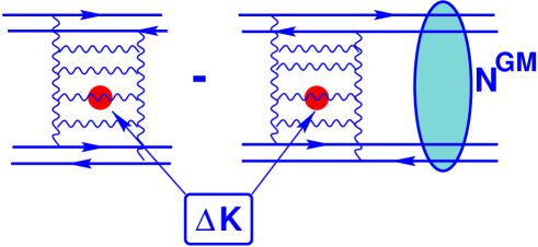
Figure 5: The diagrams for the first order correction with respect to $\Delta K$,which includes the non-perturbative QCD contribution at large values of the impact parameter.

The sum of all diagrams in Fig. 5 leads to a contribution

$$\Delta K\,\left(1\,\,-\,\,N^{GM}(x,r_{1,t},r_{2,t},b_{t})\,\right)\,\,=\,\,\Delta K\,e^{-N^{OPS}(x,r_{1,t},r_{2,t},b_{t})}$$ (4.61)

Since for $b_{t}\,<\,b_{0}(x)$ $N^{GM}$ is very close to unity, the above corrections are suppressed. Only for $b_{t}\,\geq\,b_{0}(x)$ we can expect a considerable contribution. However, this contribution is proportional to $e^{-2\,m_{\pi}\,b_{0}(x)}\,=\,e^{-\omega_{L}\ln(x_{0}/x)}$ . Therefore they turn out to be very small.

This simple discussion shows why the strategy to include the non-perturbative corrections in the Born amplitude, works

Actually, the main result of this paper, namely Eq. (3.38), is based on a simple physics (see Ref. [16]). We have demonstrated here that the multi rescattering processes embraced by the Glauber-Mueller formula lead to a different resulting parton cascade than is given by the BFKL approach. The principle difference is the fact that the multi parton shower interaction creates a new scale or mean parton transverse momentum ( saturation scale) given by Eq. (3.52).

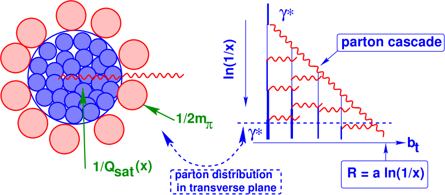
Figure 6: The structure of the parton cascade of the fast photon in the frame where the second photon is at rest. The picture is the three-dimensional one since the thickness of the vertical line reflects the value of the transverse momentum. The thicker the line the larger value of the parton transverse momentum. The left part of the picture shows the parton distribution in the transverse plane.

$N(x,r_{1,t},r_{2,t},b_{t})$ denotes the parton density, consequently the fact that $N(x,r_{1,t},r_{2,t},b_{t})\,\rightarrow\,1$ can be understood as the   fact that the partons reach a maximal density at low $x$. This phenomenon is called saturation [11, 12, 13]. Therefore, at low $x$ we have the parton distribution in the transverse plane presented in Fig. 6: the uniform distribution of partons ( dipoles) with sizes of the order of $1/Q_{sat}(x)$ in the disc of radius $R(x)$. If one of the dipole inside of the disc will emit one extra parton this emitted parton will interact with others partons and as a result of this interaction its transverse momentum will be of the order of $Q_{sat}(x)$. It means that this emitted gluon will not change its position in impact parameter space since due to uncertainty principle

$$\Delta\,b_{t}\,p_{t}\,\,\approx\,\,1$$ (4.62)

its $\Delta b_{t}\,\approx\,1/Q_{sat}(x)$. However, for the parton at the edge of the disc the situation is different since the emitted parton in the direction outside of the disc can move freely without any interaction. This parton changes the size of the disc by its displacement in $b_{t}$, namely $\Delta b_{t}\,\approx\,1/p_{t}\,\approx\,\,1/2\,m_{\pi}$. In this estimate we consider the non-perturbative emission with $p_{t}\approx 2m_{\pi}$ because, as have been discussed, a non-perturbative emission is needed to provide the unitarization of our process. Since the emission that leads to a growth of the disc occurs in one direction ( the exterior of the disc) it leads to $R\,=\,<|\Delta b_{t}|>\,n$ where $n$ is the number of emission at given $x$. Since the emission takes place at the edge of the disc where the parton density is rather small, $N(x,r_{1,t},r_{2,t},b_{t})$ is determined by the BFKL dynamics only [16, 18]. In the BFKL approach [4]$n\,=\,\omega_{l}\,\ln((x_{0}/x)$ since $N^{OPS}\,\propto\,e^{n}\,=\,e^{\omega_{l}\,\ln(x_{0}/x)}$. Therefore, we obtain Eq. (3.38), namely, $R(x)\,\equiv\,b_{0}(x)\,\,=\,\,\frac{\omega_{L}}{2\,m_{\pi}}\,\ln(x_{0}/x)$.

We have discussed in this paper the structure of dipole-dipole interaction in the Glauber-Mueller approach which is the only one on the market for the interaction of two dipoles of the same sizes. However, for two dipole with small but different sizes the non-linear evolution equation [11, 12, 13, 14] should be solved to which the BFKL emission is only an approximation in the region of small partonic densities. Comparison of the result of this paper with the dipole-dipole interaction in , so called, double log approximation [1] shows that the BFKL dynamics does not change physics at large $b_{t}$. The non-linear evolution equation at fixed $b_{t}$ was solved [29] in the case when the BFKL kernel was replaced by the double log one. The solution leads to the answer in the saturation region with geometrical scale[29, 30, 18]

$$N(x,r_{1,t},r_{2,t};b_{t})\,\,\,=F\left(\tau\,=\,\,r^{2}_{1,t}\,\,Q^{2}_{sat}(x)\,\,e^{-\,4\,m_{\pi}\,b_{t}}\,\right)\,\,.$$ (4.63)

Therefore, we believe that for the BFKL dynamics Eq. (4.63) will hold. This belief is based on the similarity between double log and BFKL approximation for $\gamma^{*}-\gamma^{*}$ processes.

Acknowledgments:

We wish to thank Jochen Bartels, Errol Gotsman and Uri Maor for very fruitful discussions on the subject.

One of us (E.L.) would like to thank the DESY Theory Group for their hospitality and creative atmosphere during several stages of this work. He is indebted to the Alexander-von-Humboldt Foundation for the award that gave him a possibility to work on low $x$ physics during the last year.

This research was supported in part by the GIF grant $\#$ I-620-22.14/1999 and by Israeli Science Foundation, founded by the Israeli Academy of Science and Humanities.

Appendix A Appendix

The integration over $R_{1}$ in Eq. (2.11) can be taken explicitly [23, 24] and Eq. (2.11) can be reduced to

$$\int\,\,d^{2}\,R_{1}\,V(r_{1,t},R_{1};\nu)\,\,V(r_{1,t},|\vec{R}_{1}\,-\,\vec{b}_{t}|;-\,\nu)\,\,=\,\,\frac{\nu^{2}}{(\frac{1}{4}\,+\,\nu^{2})^{2}}$$ (A.1)

$$c_{1}\,x^{h}\,{x^{*}}^{h}\,F(h,h,2h,x)\,F(h,h,2h,x^{*})\,\,+\,\,c_{2}x^{1-h}{x^{*}}^{1-h}F(1-h,1-h,2-2h,x)\,F(1-h,1-h,2-2h,x^{*})$$

where $F(\alpha,\beta,\gamma,z)$ is the hypergeometrical function (see Ref. [27] ); $x$ is the complex anharmonic ratio:

$$x\,\,=\,\,\frac{r_{1,t}\,r_{2,t}}{(b-z_{1}\,r_{1,t}-\bar{z}_{2}\,r_{2,t})\,(b-\bar{z}_{1}\,r_{1,t}-z_{2}\,r_{2,t})}$$ (A.2)

and $h\,=\,\frac{1}{2}\,+\,i\,\nu$. $x\,x^{*}$ gives

$$x\,x^{*}\,\,=\,\,\frac{r^{2}_{1,t}\,r^{2}_{2,t}}{(\vec{b}-z_{1}\,\vec{r}_{1,t}-\bar{z}_{2}\,\vec{r}_{2,t})^{2}\,(\vec{b}-\bar{z}_{1}\,\vec{r}_{1,t}-z_{2}\,\vec{r}_{2,t})^{2}}$$ (A.3)

One sees that Eq. (A.3) is invariant with respect to rotation in the plane.

The coefficients $c_{1}$ and $c_{2}$ have been calculated in Ref.[24] and they are equal:

$$c_{2} = \pi 2^{-1+4i\nu}\,\,\frac{\Gamma(i\nu)}{\Gamma(\frac{1}{2}+i\nu)}\,;$$ (A.4)

$$\frac{c_{1}}{c_{2}} = -\left(\frac{\Gamma(2-2h)}{\Gamma(2h)}\right)^{2}\,\left(\frac{\Gamma(h)}{\Gamma(1-h)}\right)^{4}\,;$$ (A.5)

However, one can see that Eq. (A.1) does not reproduce the Born term of Eq. (2.5) at $y=0$. To understand why it is so we should consider the vertex $V(r_{1,t},R_{1};\nu)$ in momentum representation ( see Ref. [23]), namely,

$$V(r_{1,t},Q;\nu)\,\,\,=\,\,\,\int\,d^{2}\,R_{1}\,e^{i\frac{\vec{Q}\,\cdot\,\vec{b}}{2}}\,V(r_{1,t},R_{1};\nu)\,\,.$$ (A.6)

It turns out [23] that

$$V(r_{1,t},Q;\nu)\,\,\, = \,\,\,(Q\,Q^{*})^{i\,\nu}2^{-6i\nu}\,\Gamma^{2}(1-i\nu)\,\times\,$$

$$\left(J_{-i\nu}(\frac{Q^{*}r_{1,t}}{4})\,J_{-i\nu}(\frac{Qr^{*}_{1,t}}{4})\,\,-\,\,J_{i\nu}(\frac{Q^{*}r_{1,t}}{4})J_{i\nu}(\frac{Qr^{*}_{1,t}}{4})\,\right)$$

At small $Q$ Eq. (A) leads to the following behavior of vertex $V(r-{1,t},Q;\nu)$:

$$V(r-{1,t},Q;\nu)\,\,\,\rightarrow|_{Q^{2}\,\rightarrow\,0}\,\,\,\,(\frac{r^{2}_{t}}{16})^{-i\nu}\,\left(\,1\,\,-\,\,(Q^{2})^{2i\nu}\,(\frac{r^{2}_{t}}{16})^{i2\nu}\,\right)$$ (A.8)

As have been discussed the matching with the Born approximation occurs at $i\nu\,\rightarrow\,\,\frac{1}{2}$. In this limit

$$V(r_{1,t},Q;\nu)\,\rightarrow\,\frac{r_{1,t}}{4}\,\left(\,1\,\,-\,\,Q^{2}\,\frac{r^{2}_{t}}{16}\,\right)\,\,,$$ (A.9)

which has correct analytical behavior. Actually this behavior dictates the choice of the coefficients $c_{1}$ and $c_{2}$ in Eq. (A.4) and Eq. (A.5).

However, at $-i\nu\,\rightarrow\,\,\frac{1}{2}$ the low $Q$ behavior has a singularity $1/Q^{2}$. Therefore the symmetry of Eq. (2.11) with respect to sign of $\nu$ is broken. Mueller and Tang [31] pointed out that this problem can be cured by adding to the expression of $V(r_{1,t},Q;\nu)$ of Eq. (2.13), namely,

$$V(r_{1,t},R_{1};\nu)\,\, \rightarrow \,\,V^{MT}(r_{1,t},R_{1};\nu)\,\,=$$

$$V(r_{1,t},R_{1};\nu)\,\,-\,\,\left(\frac{1}{(\vec{R}_{1}\,+\,\frac{1}{2}\,\vec{r}_{1,t})^{2}}\right)^{\frac{1}{2}\,-\,i\nu}\,\,-\,\,\left(\frac{1}{(\vec{R}_{1}\,-\,\frac{1}{2}\,\vec{r}_{1,t})^{2}}\right)^{\frac{1}{2}\,-\,i\,\nu}$$

As was found[15] such terms can be added due to gauge invariance of QCD. In momentum representation (see Eq. (A.6)) $V^{MT}(r_{1,t},Q;\nu)$ can be written as a sum of three terms as it is shown in Fig. 7.

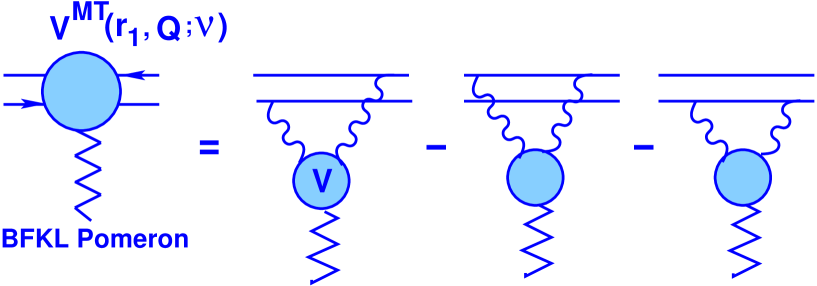
Figure 7: Structure of the Mueller-Tang vertex.

The Mueller-Tang vertex leads to the Born approximation amplitude in the form of Eq. (2.5). However, as was discussed in Refs. [15, 22, 24], it has not been proven that this vertex will satisfy the BFKL equation. The solution in the form of Eq. (A.1) has a different form of the Born amplitude, namely,

$$N^{BA}\,\propto\,\ln\left(\frac{\rho_{1,2}\,\rho_{1^{\prime},2^{\prime}}}{\rho_{1,2^{\prime}}\,\rho_{1^{\prime},2}}\right)\,\ln\left(\frac{\rho_{1,2}\,\rho_{1^{\prime},2^{\prime}}}{\rho_{1,1^{\prime}}\,\rho_{2^{\prime},2}}\right)\,\,.$$ (A.11)

However, these two expressions for the Born amplitude are equivalent due to gauge invariance of QCD [15].

Using Eq. (A.1) we can calculate the dipole-dipole amplitude at $b_{t}=0$ and, therefore, the saturation scale with better accuracy than within Eq. (3.47). On the other hand the saturation momentum increases for $x\,\rightarrow\,0$ . Such an increase guarantees that Eq. (3.47) approaches the amplitude given by Eq. (A.1) in the region of low $x$. This is the reason why we prefer to use a simple solution of Eq. (A.1) instead of full expression of Eq. (A.1).

It is easy to show that Eq. (A.1) describes all properties of diffusion approximation that has been discussed in section 2.

References

• [1] M. Kozlov and E. Levin, arXiv:hep-ph/0211348.
• [2] J. Bartels, A. De Roeck and H. Lotter, Phys. Lett. B389 (1996) 742.
• [3] S. J.  Brodsky, F. Hautmann and D.E. Soper, Phys. Rev. D56 (1997) 6957.
• [4] E.A. Kuraev, L.N. Lipatov and V.S. Fadin, Sov. Phys. JETP 45 (1977) 199;
Ia.Ia. Balitsky and L.N. Lipatov, Sov. J. Nucl. Phys. 28 (1978) 822;
L.N. Lipatov, Sov. Phys. JETP 63 (1986) 904.
• [5] A. H. Mueller, Nucl. Phys. B335 (1990) 115.
• [6] E. M. Levin and M. G. Ryskin, Sov. J. Nucl. Phys.45 (1987) 150.
• [7] A. Zamolodchikov, B. Kopeliovich and L. Lapidus, JETP Lett. 33 (1981) 595.
• [8] A. H. Mueller, Nucl. Phys. B415 (1994) 373.
• [9] A. Donnachie, H. G. Dosch and M. Rueter, Eur.  Phys.  J.  C13 (2000) 141.
• [10] N.N. Nikolaev and B.G. Zakharov, Z. Phys. C49 (1991) 607;
E.M. Levin, A.D. Martin, M.G. Ryskin and T. Teubner, Z. Phys. C74 (1997) 671.
• [11] L. V. Gribov, E. M. Levin and M. G. Ryskin, Phys. Rep. 100 (1983) 1.
• [12] A. H. Mueller and J. Qiu, Nucl. Phys. B 268 (1986) 427.
• [13] L. McLerran and R. Venugopalan, Phys. Rev. D 49 (1994) 2233, 3352; D 50 (1994) 2225, D 53 (1996) 458, D 59 (1999) 09400.
• [14] Ia. Balitsky, Nucl. Phys. B 463 (1996) 99;
Yu. Kovchegov, Phys. Rev. D 60 (2000) 034008.
• [15] L. N. Lipatov, Sov. Phys. JETP 63 (1986) 904.
• [16] E. M. Levin and M. G. Ryskin, Phys.  Rept.  189 (1990) 267.
• [17] A. Kovner and U. A. Wiedemann, “Taming the BFKL Intercept via Gluon Saturation,” hep-ph/0208265; Phys. Lett.  B551 (2003) 311 [arXiv:hep-ph/0207335]; Phys. Rev.  D66 (2002) 034031 [arXiv:hep-ph/0204277]; Phys. Rev.  D66 (2002) 051502 [arXiv:hep-ph/0112140].
• [18] E. Ferreiro, E. Iancu, K. Itakura and L. McLerran, Nucl. Phys. A 710 (2002) 373 [arXiv:hep-ph/0206241]
• [19] M. Froissart, Phys.  Rev.  123 (1961) 1053;      A.  Martin, “Scattering Theory: Unitarity, Analitysity and Crossing.” Lecture Notes in Physics, Springer-Verlag, Berlin-Heidelberg-New-York, 1969.
• [20] I. F. Ginzburg, S.L. Panfil and V.G. Serbo, Nucl. Phys. B284 (1987) 685, B296 (1988) 569;  I. F. Ginzburg and D. Yu. Ivanov, Nucl. Phys. B388 (1992) 376;   D. Y. Ivanov and R. Kirschner, Phys.  Rev.  D58 (1998) 114026, hep-ph/9807324.
• [21] P. Colangelo and A. Khodjamirian, “QCD sum rules: A modern perspective,” hep-ph/0010175;   V. E. Markushin, Acta Phys.  Polon.  B31 (2000) 2665;     O. I. Yakovlev, R. Ruckl and S. Weinzierl, “QCD sum rules for heavy flavors,” hep-ph/0007344;   M. A. Shifman, “QCD Sum Rules,” in Lenz, F. (ed.) et al.: ı“Lectures on QCD: Foundations”, pp.170-187;   S. Narison, “QCD Spectral Sum Rules,” World Sci.  Lect.  Notes Phys. , 26 (1989) 1;   M. A. Shifman, A. I. Vainshtein and V. I. Zakharov, Nucl.  Phys.  B147 (1979) 385, 448, 519.
• [22] J. Bartels, J. R. Forshaw, H. Lotter, L. N. Lipatov, M. G. Ryskin and M. Wusthoff, Phys. Lett. B348 (1995) 589 [arXiv:hep-ph/9501204].
• [23] H. Navelet and R. Peschanski, Nucl. Phys.  B634 (2002) 291 [arXiv:hep-ph/0201285];     Phys. Rev. Lett.  82 (1999) 137,, [arXiv:hep-ph/9809474];    Nucl. Phys.  B507 (1997) 353, [arXiv:hep-ph/9703238].
• [24] L. N. Lipatov, Phys. Rept.  286, 131 (1997) [arXiv:hep-ph/9610276].
• [25] J. C. Collins and J. Kwiecinski, Nucl. Phys. B 335 (1990) 89;    J. Bartels, J. Blumlein, and G. Shuler, Z. Phys. C 50 (1991) 91;    A. L. Ayala, M. B. Gay Ducati, and E. M. Levin, Nucl. Phys. B 493 (1997) 305, B 510 (1990) 355;    Yu. Kovchegov, Phys. Rev. D 54 (1996) 5463, D 55 (1997) 5445, D 61 (2000) 074018;    A. H. Mueller, Nucl. Phys. B 572 (2000) 227, B 558 (1999) 285;    Yu. V. Kovchegov, A. H. Mueller, Nucl. Phys. B 529 (1998) 451;    E. Iancu, A. Leonidov, and L. McLerran, Nucl. Phys.  A 692 (2001) 583;    M. Braun, Eur. Phys. J. C 16 (2000) 337.
• [26] J. Jalilian-Marian, A. Kovner, L. McLerran, and H. Weigert, Phys. Rev. D 55 (1997) 5414;    J. Jalilian-Marian, A. Kovner, and H. Weigert, Phys. Rev. D 59 (1999) 014015;    J. Jalilian-Marian, A. Kovner, A. Leonidov, and H. Weigert, Phys. Rev. D 59 (1999) 034007, Erratum-ibid. Phys. Rev. D 59 (1999) 099903;    A. Kovner, J.Guilherme Milhano, and H. Weigert, Phys.  Rev. D 62 (2000) 114005;   H. Weigert, Nucl.  Phys. A 703 (2002) 823.
• [27] I. Gradstein and I. Ryzhik, “ Tables of Series, Products, and Integrals”, Verlag MIR, Moskau,1981.
• [28] A. H. Mueller and D. N. Triantafyllopoulos, Nucl. Phys.  B640 (2002) 331, [arXiv:hep-ph/0205167];    D. N. Triantafyllopoulos, Nucl. Phys.  B648 (2003) 293, [arXiv:hep-ph/0209121].
• [29] E. Levin and K. Tuchin, Nucl. Phys.  B573, 833 (2000) [arXiv:hep-ph/9908317]; Nucl. Phys.  A691, 779 (2001) [arXiv:hep-ph/0012167]; Nucl. Phys. A693 (2001) 787 [arXiv:hep-ph/0101275].
• [30] J. Bartels and E. Levin, Nucl. Phys.  B387, 617 (1992). A. M. Stasto, K. Golec-Biernat and J. Kwiecinski, Phys. Rev. Lett.  86, 596 (2001) [arXiv:hep-ph/0007192];    E. Iancu, K. Itakura and L. McLerran, Nucl. Phys.  A708 (2002) 327 [arXiv:hep-ph/0203137],Phys. Lett.  B510 (2001) 145 [arXiv:hep-ph/0103032];“Understanding geometric scaling at small x,” arXiv:hep-ph/0205198.
• [31] A. H. Mueller and W. K. Tang, Phys. Lett.  B284 (1992) 123.