QCD Aspects of Exclusive $B$ Meson Decays

Abstract

I review recent progress on understanding QCD dynamics involved in exclusive $B$ meson decays. Different frameworks, including light-cone sum rules, QCD factorization, perturbative QCD, soft-collinear effective theory, light-front QCD, are discussed. Results from lattice QCD are quoted for comparison. I point out the important issues in the above QCD methods, which require further investigation.

1 Introduction

We are now in the era of $B$ physics. $B$ fatories at KEK and SLAC have collected about 80 $fb^{-1}$ data, based on which we are not only able to probe the origin of CP violation, but to explore rich QCD dynamics involved in exclusive $B$ meson decays. As announced in [1], the Kobayashi-Maskawa (KM) ansatz [2] for CP violation is more or less certain with the consistent measurements of $\sin 2\phi_{1}$ (or $\sin 2\beta$) from Belle and BaBar, $\phi_{1}$ being one of the unitarity angles. The results are also in agreement with other indirect determination of the Cabibbo-Kobayashi-Maskawa (CKM) matrix elements. In this article I will forcus on the latter subject. It will be realized that exclusive $B$ meson decays provide a unique field, in which QCD theories with controllable theoretical uncertainty can be developed. It turns out that these theories are simpler than those for charm and kaon physics. This field has attracted wide attention, and tremendous progress has been made recently.

Within the KM ansatz, the source of CP violation is organized in the form of a unitarity triangle. On one hand, we overconstrain the unitarity triangle as much as possible, and on the other hand, look for possible discrepancies, which could reveal signals of new physics beyond the Standard Model. The angle $\phi_{1}$ can be extracted from the CP asymmetry in the $B\to J/\psi K_{S}$ decays [3], which arises from the $B$-$\bar{B}$ mixing. Through similar mechanism, the $B_{d}^{0}\to\pi^{+}\pi^{-}$ decays are appropriate for the extraction of the angle $\phi_{2}$ (or $\alpha$). However, these modes contain both tree and penguin contributions, such that the extraction suffers uncertainty. Strategies have been proposed to handle this penguin pollution, the best of which is known to be the isospin analysis [4]. Unfortunately, this strategy is difficult in practice, because of the small $B_{d}^{0}\to\pi^{0}\pi^{0}$ branching ratios. The angle $\phi_{3}$ (or $\gamma$) can be determined from the decays $B\to K\pi$ [5, 6, 7, 8], which are obviously also plagued by the similar penguin-tree interference.

We can move forward by learning how to estimate hadronic matrix elements involved in exclusive $B$ meson decays. For this purpose, symmetries of strong interaction have been postulated to relate amplitudes among different modes. For example, the penguin-over-tree ratio $|P/T|$ helps the extraction of $\phi_{2}$ from the CP-violating observables in $B_{d}^{0}\to\pi^{+}\pi^{-}$ [9]. $SU(3)$ flavor symmetry and plausible dynamical assumptions were then employed to fix $|P|$ through the CP-averaged $B^{\pm}\to K\pi^{\pm}$ branching ratio [10]. The information of $|T|$ can be obtained from the $B\to\pi l\nu$ data. Another strategy is to apply the $U$-spin flavor symmetry to the $B_{d}^{0}\to\pi^{+}\pi^{-}$ and $B_{s}\to K^{+}K^{-}$ modes [11], from which the penguin amplitudes are determined. However, the above symmetries are in fact not exact, and it is not clear how to control theoretical uncertainties from symmetry breaking. As an alternative, one searches for the special modes, in which relations among decay amplitudes allow the elimination of hadronic uncertainties. For example, $\phi_{3}$ can be extracted from the triangle relations for the $B^{\pm}_{u}\to K^{\pm}\{D^{0},{\bar{D}}^{0},D^{0}_{+}\}$ amplitudes [12, 13], which receive only tree contributions, $D^{0}_{+}$ being the CP-even eigenstate of the neutral $D$-meson system. However, this strategy, due to the squashed triangles, is experimentally difficult [14]. The modes $B_{d}\to K^{\ast 0}\{D^{0},{\bar{D}}^{0},D^{0}_{+}\}$ [15] and $B^{\pm}_{c}\to D_{s}^{\pm}\{D^{0},{\bar{D}}^{0},D^{0}_{+}\}$ [16], providing more equilateral triangles, then deserve further feasibility studies.

The above discussion indicates that it is necessary to have deeper understanding of QCD dynamics in exclusive $B$ meson decays and control of hadronic uncertainties [17]. The $b$ quark mass $m_{b}$, much larger than the QCD scale $\Lambda_{\rm QCD}$, renders such an attempt possible: relevant hadronic matrix elements can be evaluated as an expansion in the strong coupling constant $\alpha_{s}(m_{b})$ and in the ratio $\Lambda_{\rm QCD}/m_{b}$. The approaches based on this heavy quark expansion include light-cone QCD sum rules (LCSR) [18, 19, 20], light-front QCD (LFQCD) [21, 22], QCD factorization (QCDF) [23], and perturbative QCD (PQCD) [24, 25, 26]. Soft-collinear effective theory (SCET) provides a systematic framework, in which the above expansion can be constructed in a simple and formal way [27, 28]. Lattice QCD is complementary to the above methods, whose results will be quoted for comparison. In this article I will explain the basic ideas behind the various QCD theories, and review their applications to typical, such as semileptonic, radiative and nonleptonic, exclusive modes. That is, I emphasize the methodology, instead of the survey of all decay channels.

To be specific, I will not discuss the strategies to constrain the CKM matrix elements from experimental data. For nice reviews of this topic, refer to [29, 30, 31]. I will not explore analyses relying on symmetries of strong interaction, such as the $SU(3)$ flavor symmetry. Recent works along this vein, which have taken into account symmetry breaking effects, can be found in [32, 33, 34]. The status of the important CKM global fitting have been presented in [35, 36]. To demonstrate the applications of the QCD methods, I will consider only $B_{u,d}$ meson decays as an example. The subjects related to the $B_{s}$ and $B_{c}$ mesons and to heavy baryons, including their polarization effect, will be dropped. The perspectives for investigating $B_{c}$ mesons at LHCb have been surveyed in [37]. For a similar reason, I skip the applications to decays into baryons and into tensor mesons [38]. Studies of three-body $B$ meson decays are still at the early stage [39, 40], and will be reserved for a future review. I will not touch supersymmetric topics in $B$ physics either, which are too much for this article. For a recent relevant review, refer to [41, 42].

In Sec. 2 and Sec. 3 I briefly explain two types of factorization theorems, collinear and $k_{T}$ factorizations, which are the fundamental concepts of most of the QCD theories. The ideas and results derived from the various QCD methods are reviewed in Sec. 4 for semileptonic and radiative decays, and in Sec. 5 for two-body nonleptonic decays. Charmed decays are discussed in Sec. 6. Other miscellaneous topics are collected in Sec. 7. Section 8 is the conclusion.

2 Collinear Factorization

Most of QCD methods rely on some sorts of factorization theorems. For example, QCDF is a generalization of collinear factorization theorem to exclusive $B$ meson decays. In LCSR collinear factorization applies to final-state hadron bound states, which are then expanded in terms of parton Fock states characterized by different twists. $k_{T}$ factorization theorem is the basis of the PQCD approach, which is more appropriate in the end-point region of parton momentum fractions. SCET for the kinematic region with energetic final-state hadrons, is equivalent to collinear factorization theorem, but operated at the operator and Lagrange level. I will compare the factorization of high-energy QCD processes derived from perturbation theory and from SCET. I then discuss the double logarithmic resummation, which is required for applying collinear factorization theorem to semileptonic $B$ meson decays.

2.1 Factorization Theorem

I first review collinear factorization theorem for exclusive processes developed around 80’s [43, 44, 45, 46, 47, 48]. In this theorem nonperturbative dynamics of a high-energy QCD process, characterized by a large scale $Q$, either cancel or is absorbed into hadron distribution amplitudes. The remaining part, being infrared finite, is calculable in perturbation theory. A physical quantity is then expressed as the convolution of a hard-scattering kernel with the distribution amplitudes solely in parton momentum fractions. A distribution amplitude, though not calculable, is universal, i.e., process-independent. With this universality, a distribution amplitude determined by nonperturbative means, such as QCD sum rules and lattice QCD, or extracted from experimental data, can be employed to make predictions for other processes involving the same hadron. Contributions of different orders in $\alpha_{s}$ and powers in $1/Q$ can be included systematically.

Nonperturbative dynamics is reflected by infrared divergences in radiative corrections, whose factorization leads to distribution amplitudes at the parton level. Factorization of the above infrared divergences needs to be performed in momentum, spin, and color spaces. Factorization in momentum space means that a hard kernel depends on the loop momentum of a soft or collinear gluon, which has been absorbed into a distribution amplitude, only through the parton momentum fraction. Factorization in spin and color spaces means that there are separate fermion and color flows between a hard kernel and a distribution amplitude, respectively. I take the simple process $\pi\gamma^{*}\to\gamma$ as an example to demonstrate the proof of collinear factorization thheorem based on perturbation theory. The collinear factorization of this process has been proved in [43], but in the axial (light-cone) gauge $A^{+}=0$. In this gauge factorization automatically holds and the analysis is straightforward, because collinear divergences exist only in two-parton reducible diagrams. The pion distribution amplitude has been constructed from $\gamma^{*}\gamma\to\pi$ in the framework of covariant operator product expansion [44, 45]. The factorization of $\pi\gamma^{*}\to\pi$ has been proved in [46] based on the Zimmermann’s ”$\Delta$-forest” prescription [49], which involves complicated diagram subtractions.

Below I will adopt a simple proof proposed in [50]. To achieve factorization in momentum, spin, and color spaces, one needs the eikonal approximation for loop integrals in leading infrared regions, the insertion of the Fierz identity to separate fermion flows, and the Ward identity to sum up diagrams with different color structures. Under the eikonal approximation, a soft or collinear gluon is detached from the lines in a hard kernel and in other distribution amplitudes. The Fierz identity decomposes the full amplitude into contributions characterized by different twists. The Ward identity is essential for proving factorization theorem in a nonabelian gauge theory. The soft divergences exist in exclusive $B$ meson decays, which should be factorized into a $B$ meson distribution amplitude. The derivation in [50] is explicitly gauge-invariant, and appropriate for both the factorizations of soft and collinear divergences, compared to those in the literature.

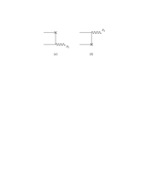
Figure 1: Lowest-order diagrams for $\pi\gamma^{*}\to\gamma$ ($B\to\gamma l\bar{\nu}$), where the symbol $\times$ represents the virtual photon (weak decay) vertex.

The momentum $P_{1}$ of the pion and the momentum $P_{2}$ of the outgoing on-shell photon are chosen, in light-cone coordinates, as

$$P_{1}=(P_{1}^{+},0,{\bf 0}_{T})=\frac{Q}{\sqrt{2}}(1,0,{\bf 0}_{T})\;,\;\;\;\;P_{2}=(0,P_{2}^{-},{\bf 0}_{T})=\frac{Q}{\sqrt{2}}(0,1,{\bf 0}_{T})\;.$$ (1)

Let $\epsilon$ denote the polarization vector of the outgoing photon, which contains only the transverse components. Consider the kinematic region with large $Q^{2}=-q^{2}$, $q=P_{2}-P_{1}$ being the virtual photon momentum, where perturbative expansion is reliable. The lowest-order diagrams are displayed in Fig. 1. Assume that the on-shell quark and antiquark carry the fractional momenta ${\bar{x}}P_{1}$ and $xP_{1}$, respectively, with ${\bar{x}}\equiv 1-x$. Figure 1(a) gives the parton-level amplitude,

$${\cal G}^{(0)}(x)=-ie^{2}{\bar{q}}(xP_{1})\not\epsilon\frac{\not P_{2}-x\not P_{1}}{(P_{2}-xP_{1})^{2}}\gamma_{\mu}q({\bar{x}}P_{1})\;.$$ (2)

The analysis for Fig. 1(b) is the same. The internal quarks are regarded as being hard, i.e., being off-shell by $O(Q^{2})$.

The factorization in the fermion flow is achieved by inserting the Fierz identity,

$$I_{ij}I_{lk}=\frac{1}{4}I_{ik}I_{lj}+\frac{1}{4}(\gamma_{5})_{ik}(\gamma_{5})_{lj}+\frac{1}{4}(\gamma_{\alpha})_{ik}(\gamma^{\alpha})_{lj}+\frac{1}{4}(\gamma_{5}\gamma^{\alpha})_{ik}(\gamma_{\alpha}\gamma_{5})_{lj}+\frac{1}{8}(\sigma^{\alpha\beta})_{ik}(\sigma_{\alpha\beta})_{lj}\;,$$ (3)

where $I$ represents the identity matrix, and $\sigma_{\alpha\beta}$ is defined as $\sigma_{\alpha\beta}\equiv i[\gamma_{\alpha},\gamma_{\beta}]/2$. Different terms in the above identity lead to contributions of different twists. Equation (2) is then factorized into

$${\cal G}^{(0)}(x)=\int d\xi\phi^{(0)}(x,\xi){\cal H}^{(0)}(\xi)\;,$$ (4)

where the functions,

$$\phi^{(0)}(x,\xi) = \phi^{(0)}(x)\delta(x-\xi)\;,\;\;\;\;\phi^{(0)}(x)=\frac{1}{4P_{1}^{+}}{\bar{q}}(xP_{1})\gamma_{5}\not{\bar{n}}q({\bar{x}}P_{1})\;,$$

$${\cal H}^{(0)}(x) = ie^{2}\frac{tr(\not\epsilon\not P_{2}\gamma_{\mu}\not P_{1}\gamma_{5})}{2xP_{1}\cdot P_{2}}\;,$$ (5)

with the dimensionless vector $\bar{n}=(0,1,{\bf 0}_{T})$ on the light cone, define the lowest-order distribution amplitude and hard kernel in perturbation theory, respectively. For the momenta chosen in Eq. (1), only the pseudo-vector structure $\gamma_{\alpha}\gamma_{5}$ with $\alpha=+$ survives, as it is contracted with the hard kernel to form the factor $\not P_{1}\gamma_{5}$ in Eq. (5). This piece of contribution is of leading twist (twist 2). For other processes, such as the pion form factor, higher-twist structures survive, but the analysis is the same [50].

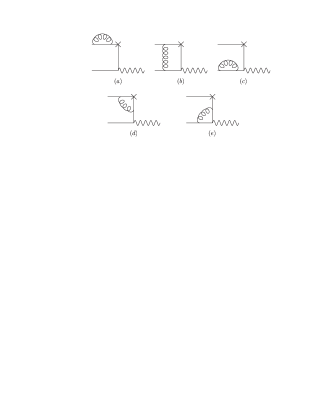
Figure 2: $O(\alpha_{s})$ radiative corrections to Fig. 1(a).

There are two types of infrared divergences in radiative corrections, soft and collinear. In the soft region and in the collinear region associated with the pion momentum $P_{1}$, the components of a loop momentum $l$ behave like

$$l^{\mu}=(l^{+},l^{-},{\bf l}_{T})\sim Q(\lambda,\lambda,\lambda)\;,\;\;\;\;l^{\mu}\sim Q(1,\lambda^{2},\lambda)\;,$$ (6)

respectively, where $\lambda$ is a small parameter. In both regions the invariant mass of the radiated gluon diminishes as $\lambda^{2}$, and the corresponding loop integrand may diverge as $1/\lambda^{4}$. As the phase space for loop integration vanishes like $d^{4}l\sim\lambda^{4}$, logarithmic divergences are generated.

We identify the infrared divergences in the $O(\alpha_{s})$ corrections [51, 52, 53] to Fig. 1(a), which are shown in Fig. 2. Self-energy correction to the internal quark, giving a next-to-leading-order hard kernel, is not included. The collinear factorization formula is written as the convolution over the momentum fraction $\xi$,

$${\cal G}^{(1)}(x) = \sum_{i=a}^{e}{\cal G}^{(1)}_{i}(x)\;,$$

$${\cal G}^{(1)}_{i}(x) = \int d\xi\phi_{i}^{(1)}(x,\xi){\cal H}^{(0)}(\xi)+\phi^{(0)}(x){\cal H}_{i}^{(1)}(x)\;,$$ (7)

The above expression, with the $O(\alpha_{s})$ distribution amplitudes $\phi_{i}^{(1)}(x,\xi)$ specified, defines the $O(\alpha_{s})$ hard kernels ${\cal H}_{i}^{(1)}(x)$, which do not contain collinear divergences. This procedure is referred to as matching the effective theory to the full thoery in the determination of Wislon coefficients in SCET. It is now obvious why an arbitrary $x$ is considered for the parton-level diagrams in Figs. 1 and 2: one can obtain the functional form of ${\cal H}_{i}^{(1)}(x)$ in $x$.

Figures 2(a)-2(c) are the two-particle reducible diagrams with the additional gluon attaching the two valence quarks of the pion. It has been known that soft divergences cancel among these diagrams [50]. The reason for this cancellation is that soft gluons, being huge in space-time, do not resolve the color structure of the pion. Collinear divergences in Figs. 2(a)-2(c) do not cancel, since the loop momentum flows into the internal quark line in Fig. 2(b), but not in Figs. 2(a) and 2(c). To absorb the collinear divergences, one introduces a nonperturbative distribution amplitude. The factorization of the above diagrams is achieved by inserting the Fierz identity. For example, one obtains, from Fig. 2(b), the $O(\alpha_{s})$ distribution amplitude,

$$\phi^{(1)}_{b}(x,\xi)=\frac{ig^{2}C_{F}}{4P_{1}^{+}}\int\frac{d^{4}l}{(2\pi)^{4}}{\bar{q}}(xP_{1})\frac{\gamma^{\nu}(x\not P_{1}-\not l)\gamma^{5}\not{\bar{n}}({\bar{x}}\not P_{1}+\not l)\gamma_{\nu}}{(xP_{1}-l)^{2}({\bar{x}}P_{1}+l)^{2}l^{2}}q({\bar{x}}P_{1})\delta\left(\xi-x+\frac{l^{+}}{P_{1}^{+}}\right)\;,$$ (8)

with $C_{F}=4/3$ being a color factor. $\phi^{(1)}_{b}$ contains the collinear divergence, because the integrand in Eq. (8) diverges as $1/\lambda^{4}$. The dependences on $l^{-}$ and on $l_{T}$ in ${\cal H}^{(0)}$, being subleading according to Eq. (6), have been neglected.

In the collinear region of Fig. 2(d), the following approximation for part of the loop integrand holds,

$$(\not P_{2}-x\not P_{1})\gamma^{\nu}(\not P_{2}-x\not P_{1}+\not l) \approx 2P_{2}^{\nu}\not P_{2}\;,$$ (9)

where the $l^{-}$ and $l_{T}$ terms, being power-suppressed compared to $P_{2}^{-}$, have been dropped. The factorization of the collinear divergence from Figs. 2(d) requires the further approximation for the product of the two internal quark propagators [50],

$$\frac{2P_{2}^{\nu}}{(P_{2}-xP_{1})^{2}(P_{2}-xP_{1}+l)^{2}}\approx\frac{\bar{n}^{\nu}}{\bar{n}\cdot l}\biggl{[}\frac{1}{(P_{2}-xP_{1})^{2}}-\frac{1}{(P_{2}-xP_{1}+l)^{2}}\biggr{]}\;,$$ (10)

which is an example of the Ward identity. Similarly, the power-suppressed terms, such as $l^{2}$ and $xP_{1}\cdot l$, have been neglected . The numerator $2P_{2}^{\nu}$ comes from Eq. (9), and the factor $\bar{n}^{\nu}/\bar{n}\cdot l$ is exactly the Feynman rule associated with a Wilson line. Therefore, the appearence of the Wilson line is a consequence of the Ward identity.

The first (second) term on the right-hand side of Eq. (10) corresponds to the case without (with) the loop momentum $l$ flowing through the hard kernel. Hence, the extracted $O(\alpha_{s})$ distribution amplitude is written as

$$\phi^{(1)}_{d}(x,\xi) = \frac{-ig^{2}C_{F}}{4P_{1}^{+}}\int\frac{d^{4}l}{(2\pi)^{4}}{\bar{q}}(xP_{1})\gamma^{5}\not{\bar{n}}\frac{{\bar{x}}\not P_{1}+\not l}{({\bar{x}}P_{1}+l)^{2}}\gamma_{\nu}q({\bar{x}}P_{1})\frac{1}{l^{2}}\frac{\bar{n}^{\nu}}{\bar{n}\cdot l}$$ (11)

$$\times\left[\delta(\xi-x)-\delta\left(\xi-x+\frac{l^{+}}{P_{1}^{+}}\right)\right]\;,$$

where the first (second) term in the bracket is associated with the first (second) term on the right-hand side of Eq. (10). The factorization of the distribution amplitude from Figs. 2(e) is performed in a similar way.

The above $O(\alpha_{s})$ distribution amplitudes can be reproduced by the $O(\alpha_{s})$ terms of the following nonlocal matrix element with the structure $\gamma_{5}\not{\bar{n}}$ sandwiched,

$$\phi(x,\xi)=i\int\frac{dy^{-}}{2\pi}e^{-i\xi P_{1}^{+}y^{-}}\langle 0|{\bar{q}}(y^{-})\gamma_{5}\not{\bar{n}}{\cal P}\exp\left[-ig\int_{0}^{y^{-}}dz\bar{n}\cdot A(z\bar{n})\right]q(0)|{\bar{q}}(xP_{1})q({\bar{x}}P_{1})\rangle\;.$$ (12)

The notation $\cal P$ means the path ordering for the Wilson line. The integral over $z$ contains two pieces: to generate the first term in Eq. (11), $z$ runs from 0 to $\infty$; to generate the second term, $z$ runs from $\infty$ back to $y^{-}$. The light-cone coordinate $y^{-}\not=0$ corresponds to the fact that the collinear divergences in Fig. 2 do not cancel. The Wilson line along the light cone collects collinear gluons in irreducible diagrams. By expanding the quark field ${\bar{q}}(y^{-})$ and the Wilson line into powers of $y^{-}$, the above matrix element can be expressed as a series of covariant derivatives $(D^{+})^{n}{\bar{q}}(0)$, $D=\partial-igA$, implying that Eq. (12) is gauge-invariant.

I then review the all-order proof of leading-twist collinear factorization theorem for the process $\pi\gamma^{*}\to\gamma$, and justify the definition of the parton-level distribution amplitude in Eq. (12). The proof is performed in the covariant gauge, in which collinear divergences also exist in two-particle irreducible diagrams. It has been mentioned that factorization of a QCD process in momentum, spin, and color spaces requires summation of many diagrams, especially at higher orders. Hence, the diagram summation must be handled in an elegant way. For this purpose, one employs the Ward identity,

$$l_{\mu}G^{\mu}(l,k_{1},k_{2},\cdots,k_{n})=0\;,$$ (13)

where $G^{\mu}$ represents a physical amplitude with an external gluon carrying the momentum $l$ and with $n$ external quarks carrying the momenta $k_{1}$, $k_{2}$, $\cdots$, $k_{n}$. All these external particles are on mass shell. The Ward identity can be easily derived by means of the Becchi-Rouet-Stora (BRS) transformation [54].

Factorization theorem can be proved by induction. The factorization of the $O(\alpha_{s})$ collinear divergences associated with the pion has been worked out in Eq. (7). Assume that factorization theorem holds up to $O(\alpha_{s}^{N})$,

$${\cal G}^{(j)}(x)=\sum_{i=0}^{j}\int d\xi\phi^{(i)}(x,\xi){\cal H}^{(j-i)}(\xi)\;,\;\;\;\;j=1,\cdots,N\;,$$ (14)

where $\phi^{(i)}(x,\xi)$ is given by the $O(\alpha_{s}^{i})$ terms in the perturbative expansion of Eq. (12), and ${\cal H}^{(j-i)}(\xi)$ stands for the $O(\alpha_{s}^{j-i})$ infrared-finite hard kernel. It will be shown that the $O(\alpha_{s}^{N+1})$ diagrams ${\cal G}^{(N+1)}$ is written as the convolution of the $O(\alpha_{s}^{N})$ diagrams ${\cal G}^{(N)}$ with the $O(\alpha_{s})$ distribution amplitude by employing the Ward identity in Eq. (13).

Look for the gluon in a complete set of $O(\alpha_{s}^{N+1})$ diagrams ${\cal G}^{(N+1)}$, one of whose ends attaches the outer most vertex on the upper quark line in the pion. Let $\alpha$ denote the outer most vertex, and $\beta$ denote the attachments of the other end of the identified gluon inside the rest of the diagrams. There are two types of collinear configurations associated with this gluon, depending on whether the vertex $\beta$ is located on an internal line with a momentum along $P_{1}$. The quark spinor adjacent to the vertex $\alpha$ is $q({\bar{x}}P_{1})$. If $\beta$ is not located on a collinear line along $P_{1}$, the component $\gamma^{+}$ in $\gamma^{\alpha}$ and the minus component of the vertex $\beta$ give the leading contribution. If $\beta$ is located on a collinear line along $P_{1}$, $\beta$ can not be minus, and both $\alpha$ and $\beta$ label the transverse components. This configuration is the same as of the self-energy correction to an on-shell particle.

According to the above classification, one decomposes the tensor $g_{\alpha\beta}$ appearing in the propagator of the identified gluon as

$$g_{\alpha\beta}=\frac{\bar{n}_{\alpha}l_{\beta}}{\bar{n}\cdot l}-\delta_{\alpha T}\delta_{\beta T}+\left(g_{\alpha\beta}-\frac{\bar{n}_{\alpha}l_{\beta}}{\bar{n}\cdot l}+\delta_{\alpha T}\delta_{\beta T}\right)\;.$$ (15)

The first term on the right-hand side extracts the first type of collinear enhancements, since the light-like vector $\bar{n}_{\alpha}$ selects the plus component of $\gamma^{\alpha}$, and the dominant component $l_{\beta=-}$ in the collinear region selects the minus component of the vertex $\beta$. The components $l_{\beta=+,T}$ do not change the collinear structure, since they are negligible in the numerators compared to the leading terms proportional to $P_{1}^{+}$ or $P_{2}^{-}$. This can be confirmed by contracting $l_{\beta}$ to Fig. 2(d), from which Eq. (10) is obtained. The second term extracts the second type of collinear enhancements. The last term does not contribute a collinear enhancement due to the equation of motion for the valence quark. We shall concentrate on the factorization of ${\cal G}_{\parallel}^{(N+1)}$ corresponding to the first term on the right-hand side of Eq. (15), and the factorization associated with the second term can be included following the procedure in [50].

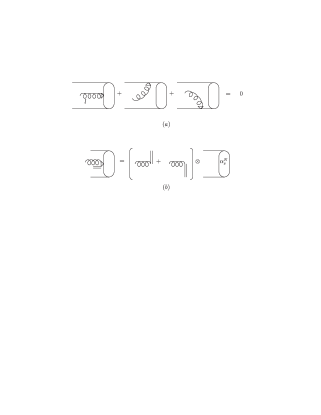
Figure 3: (a) Ward identity. (b) Factorization of ${\cal G}^{(N+1)}$.

The contraction of $l_{\beta}$ hints the application of the Ward identity in Eq. (13) to the case with two external on-shell quarks. Those diagrams with Figs. 2(a) and 2(b) as the $O(\alpha_{s})$ subdiagrams are excluded from the set of ${\cal G}_{\parallel}^{(N+1)}$ as discussing the first type of collinear configurations, since the identified gluon does not attach a line parallel to $P_{1}$. Consider the physical amplitude, in which the two on-shell quarks and the on-shell gluon carry the momenta ${\bar{\xi}}P_{1}$, $xP_{1}$ and $l$, respectively. Figure 3(a), describing the Ward identity, contains a complete set of contractions of $l_{\beta}$, since the second and third diagrams have been added back. The second and third diagrams in Fig. 3(a) lead to

$$l_{\beta}\frac{1}{{\bar{\xi}}\not P_{1}-\not l}\gamma^{\beta}q({\bar{\xi}}P_{1})=\frac{1}{{\bar{\xi}}\not P_{1}-\not l}(\not l-{\bar{\xi}}\not P_{1}+{\bar{\xi}}\not P_{1})q({\bar{\xi}}P_{1})=-q({\bar{\xi}}P_{1})\;,$$

$$l_{\beta}{\bar{q}}(xP_{1})\gamma^{\beta}\frac{1}{x\not P_{1}-\not l}=-{\bar{q}}(xP_{1})\;,$$ (16)

respectively. The terms $q({\bar{\xi}}P_{1})$ and ${\bar{q}}(xP_{1})$ at the ends of the above expressions correspond to the $O(\alpha_{s}^{N})$ diagrams.

Figure 3(b) shows that the diagrams ${\cal G}_{\parallel}^{(N+1)}$ associated with the first term in Eq. (15) are factorized into the convolution of the parton-level $O(\alpha_{s}^{N})$ diagrams ${\cal G}^{(N)}$ with the $O(\alpha_{s})$ collinear piece extracted from Fig. 2(d). The factor $\bar{n}_{\alpha}/\bar{n}\cdot l$ from the collinear replacement in Eq. (15) is exactly the Feynman rule associated with the Wilson line in the direction of $\bar{n}$, represented by the double line. The first diagram means that the gluon momentum does not flow into ${\cal G}^{(N)}$, while in the second diagram the gluon momentum does. The similar reasoning applies to the identified gluon, one of whose ends attaches the outer most vertex of the lower antiquark line. Substituting Eq. (14) into ${\cal G}^{(N)}(\xi)$ on the right-hand side of Fig. 3(b), and following the procedure in [50], one arrives at

$${\cal G}^{(N+1)}(x)=\sum_{i=0}^{N+1}\int d\xi\phi^{(i)}(x,\xi){\cal H}^{(N+1-i)}(\xi)\;,$$ (17)

with the infrared-finite $O(\alpha_{s}^{N+1})$ hard kernel ${\cal H}^{(N+1)}$. Equation (17) implies that all the collinear enhancements in the process $\pi\gamma^{*}\to\gamma$ can be factorized into the distribution amplitude in Eq. (12) order by order.

Equation (12) plays the role of an infrared regulator for the parton-level diagrams. A hard kernel ${\cal H}(x,Q^{2},\mu)$ can then be regarded as the regularized parton-level diagrams, where the dependences on the momentum transfer $Q$ and on the factorization scale $\mu$ have been made explicit. Different choices of $\mu$ correspond to different factorization schemes. Since the parton-level diagrams with on-shell external particles and Eq. (12) are both gauge-invariant, the hard kernel is gauge-invariant. After determining the gauge-invariant infrared-finite hard kernel, one convolutes it with the physical two-parton pion distribution amplitude, whose all-order gauge-invariant definition is given by

$$\phi_{\pi}(x,\mu)=i\int\frac{dy^{-}}{2\pi}e^{-ixP_{1}^{+}y^{-}}\langle 0|{\bar{q}}(y^{-})\gamma_{5}\not{\bar{n}}{\cal P}\exp\left[-ig\int_{0}^{y^{-}}dz\bar{n}\cdot\cdot A(z\bar{n})\right]q(0)|\pi(P_{1})\rangle\;.$$ (18)

The valence-quark state $|{\bar{q}}(xP_{1})q({\bar{x}}P_{1})\rangle$ has been replaced by the pion state $|\pi(P_{1})\rangle$, and the pion decay constant $f_{\pi}$ has been omitted. Equation (18) can also be derived in SCET as argued in the next subsection. The $\pi\gamma^{\ast}\to\gamma$ scattering amplitude is then expressed as the convolution over the parton momentum fraction $x$,

$${\cal M}(Q^{2})=\int_{0}^{1}dx\phi_{\pi}(x,\mu){\cal H}(x,Q^{2},\mu)\;.$$ (19)

Hence, predictions derived from collinear factorization theorem are gauge-invariant and infrared-finite.

2.2 Soft-Collinear Effective Theory

Final-state hadrons in exclusive $B$ meson decays may carry energy $E$ of $O(m_{B})$, $m_{B}$ being the $B$ meson mass, which is much larger than $\Lambda_{\rm QCD}$. These processes can be analyzed in the collinear factorization framework discussed in the previous subsection. To study the collinear factorization at the operator and Lagrange level, SCET has been developed [27, 28, 55, 56]. After integrating out short-distance fluctuations characterized by the invariant mass $p^{2}\gg(E\lambda)^{2}$, which appear in Wilson coefficients, long-distance fluctuations are then described by new effective degrees of freedom. SCET then exhibits symmetries in the large energy limit, such as the reduction of spin structures, helicity constraints, and collinear gauge invariance, which apply to the new effective fields. Power corrections in SCET are included in terms of the small parameter $\lambda=\Lambda_{\rm QCD}/E$ (or $\lambda=\sqrt{\Lambda_{\rm QCD}/E}$) [57, 58, 59]. For a recent review, refer to [60].

The effective fields contain collinear quarks and gluons ($\xi_{n,p}$, $A_{n,q}^{\mu}$), massless soft quarks and gluons ($q_{s}$, $A_{s}^{\mu}$), and massless ultrasoft (usoft) quarks and gluons ($q_{us}$, $A_{us}^{\mu}$). The collinear fields, labelled by the light cone direction $n=(1,0,{\bf 0}_{T})$ and their momentum $p$, come from the phase redefinitions,

$$\phi_{n}(x)=\sum_{p}e^{-ip\cdot x}\phi_{n,p}(x)\;.$$ (20)

Derivatives on the collinear fields, $\partial^{\mu}\phi_{n,p}(x)\sim(E\lambda^{2})\phi_{n,p}(x)$, pick up only the small scale. The large momenta are picked up by introducing the label operator, $\bar{\cal P}\xi_{n,p}=({\bar{n}}\!\cdot\!p)\xi_{n,p}$. Similarly, the operators ${\cal P}_{T}^{\mu}$ and ${\cal P}^{\mu}$ are defined to pick up the $O(\lambda)$ labels of the collinear and soft fields, respectively. In the discussion in Sec. 2.1 the usoft fields can be regarded as the leftover pieces with the collinear or soft dynamics being factorized out. That is, the usoft fields, due to their slow variation, appear as the background fields to the collinear or soft ones.

The collinear Wilson line $W[{\bar{n}}\cdot A_{n,q}]$ and soft Wilson line $S_{n}[n\cdot A_{s}]$ are induced to preserve gauge invariance [28, 56]. For the former, the explicit expression is given by

$$W = \sum_{\rm perms}\exp\Big{[}-\frac{g}{\bar{\cal P}}\>{\bar{n}}\cdot A_{n,q}(x)\Big{]}\;,$$ (21)

which is equivalent to that in Eq. (18) derived from perturbation theory. The meaning of a collinear Wilson line in the definition of the pion distribution amplitude has been emphasized in Sec. 2.1. The usoft Wilson line $Y_{n}[n\cdot A_{us}]$ is introduced by the further field redefinitions $\xi_{n,p}=Y_{n}\xi^{(0)}_{n,p}$ and $A_{n,q}=Y_{n}A_{n,q}^{(0)}Y_{n}^{\dagger}$.

Assuming the action for the kinetic terms in SCET to be of $O(\lambda^{0})$, the scaling of each effective field in $\lambda$ can be defined straightforwardly. The power counting rules for the momenta, fields, momentum label operators, and collinear, soft and usoft Wilson lines are summarized in Table 1 [27, 28]. It is found that the scaling of the collinear and soft momenta in SCET is the same as that defined in Eq. (6). The usoft momentum in the framework based on perturbation theory will appear as discussing the factorization of soft divergence from exclusive $B$ meson decays in Sec. 3.2.

Type	Momenta $(+,-,T)$	Field Scaling	Operators
collinear	$p^{\mu}\sim(1,\lambda^{2},\lambda)$	$\xi_{n,p}\sim\lambda$	$\bar{\cal P}$, $W$ $\sim\lambda^{0}$
		($A_{n,p}^{+}$, $A_{n,p}^{-}$, $A_{n,p}^{T}$) $\sim$ (1,$\lambda^{2}$,$\lambda$)	${\cal P}_{T}^{\mu}\sim\lambda$
soft	$p^{\mu}\sim(\lambda,\lambda,\lambda)$	$q_{s,p}\sim\lambda^{3/2}$	$S_{n}\sim\lambda^{0}$
		$A_{s,p}^{\mu}\sim\lambda$	${\cal P}^{\mu}\sim\lambda$
usoft	$k^{\mu}\sim(\lambda^{2},\lambda^{2},\lambda^{2})$	$q_{us}\sim\lambda^{3}$	$Y_{n}\sim\lambda^{0}$
		$A_{us}^{\mu}\sim\lambda^{2}$

Table 1: Power counting rules for momenta, fields, momentum label operators ($\bar{\cal P},{\cal P}_{T}^{\mu}$, ${\cal P}^{\mu}$), and collinear, soft and usoft Wilson lines ($W$, $S_{n}$, $Y_{n}$) in SCET.

The leading-order Lagrangians for (u)soft light quarks and gluons are the same as in QCD. For heavy quarks $h_{v}$ labelled by the velocity $v$, we have the heavy quark effective theory (HQET) Lagrangian [61],

$${\cal L}=\bar{h}_{v}\,iv\cdot D\,h_{v}+\ldots\;.$$ (22)

The collinear quark Lagrangian can be expanded as

$${\cal L}_{c} = {\cal L}_{c}^{(0)}+{\cal L}_{c}^{(1)}+{\cal L}_{c}^{(2)}+\ldots\,.$$ (23)

The first three terms are

$${\cal L}_{c}^{(0)} = \bar{\xi}_{n,p^{\prime}}\>\bigg{\{}i\,n\cdot D\!+\!gn\cdot A_{n,q}+\Big{(}{\cal{P\!\!\!\!\hskip 1.13791pt/}}_{T}\!+gA\!\!\!/_{n,q}^{T}\Big{)}\,W\frac{1}{\bar{\cal P}}W^{\dagger}\,\Big{(}{\cal{P\!\!\!\!\hskip 1.13791pt/}}_{T}\!+gA\!\!\!/_{n,q^{\prime}}^{T}\Big{)}\bigg{\}}\frac{\bar{n}\!\!\!/}{2}\,\xi_{n,p}\,,$$

$${\cal L}_{c}^{(1)} = \bar{\xi}_{n,p^{\prime}}\bigg{\{}iD\!\!\!\!/_{T}W\frac{1}{\bar{\cal P}}W^{\dagger}\,\big{(}{\cal{P\!\!\!\!\hskip 1.13791pt/}}_{T}\!+gA\!\!\!/_{n,q^{\prime}}^{T}\big{)}+\Big{(}{\cal{P\!\!\!\!\hskip 1.13791pt/}}_{T}\!+gA\!\!\!/_{n,q}^{T}\Big{)}\,W\frac{1}{\bar{\cal P}}W^{\dagger}\,iD\!\!\!\!/_{T}\bigg{\}}\frac{\bar{n}\!\!\!/}{2}\,\xi_{n,p}\,,$$

$${\cal L}_{c}^{(2)} = \bar{\xi}_{n}\left\{iD\!\!\!\!/_{T}W\frac{1}{\bar{\cal P}}W^{\dagger}iD\!\!\!\!/_{T}-\Big{(}{\cal{P\!\!\!\!\hskip 1.13791pt/}}_{T}\!+gA\!\!\!/_{n,q}^{T}\Big{)}W\frac{1}{\bar{\cal P}}W^{\dagger}({\bar{n}}\cdot iD)W\frac{1}{\bar{\cal P}}W^{\dagger}\Big{(}{\cal{P\!\!\!\!\hskip 1.13791pt/}}_{T}\!+gA\!\!\!/_{n,q}^{T}\Big{)}\right\}\frac{\bar{n}\!\!\!/}{2}\xi_{n}\,,$$ (24)

with $D^{\mu}=\partial^{\mu}-igA^{\mu}_{us}$, where ${\cal L}_{c}^{(0)}$ gives the order $O(\lambda^{0})$ interactions [28, 55], and the expressions of ${\cal L}_{c}^{(1)}$ and of ${\cal L}_{c}^{(2)}$ were derived in [57] and in [62], respectively. For the mixed effects, which are power-suppressed, the usoft-collinear Lagrangian has been derived up to $O(\lambda^{2})$ [63]. Note that the results in [63] represent an expansion of SCET in the hybrid momentum-position space. A manifestly gauge-invariant expansion in the position space has been derived [64], in which each operator has a homogeneous power counting in $\lambda$.

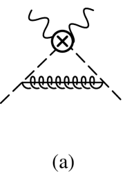
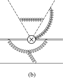
Figure 4: Diagrams for comparing the power counting in SCET and in perturbation theory for the processes (a) DIS and (b) $B\to D\pi$, respectively. Dashed lines are collinear quarks, double solid lines are usoft or soft heavy quarks, and the single solid lines are soft light quarks. Gluons with a line through them are collinear, while those without a line are soft or usoft.

After defining the power counting rules, I explain how to construct collinear factorization theorem at the operator and Lagrange level. The idea is to start with an operator relevant for a high-energy QCD process, which is characterized by some power of $\lambda$. Draw the diagrams based on this operator and the effective Lagrangians in Eqs. (22) and (23). The power of a diagram is the sum of those for the loop measures, propagators, vertices, and external lines. Note that powers in $\lambda$ shift between the propagators and vertices in different gauges. I will adopt the Feynman gauge the same as in Sec. 2.1 in order to compare the formalism in SCET and in perturbation theory. Those diagrams, whose contributions scale like the power the same as of the specified operator, contribute to the corresponding matrix element.

Consider the diagrams in Fig. 4. The one-loop diagram in Fig. 4(a) involves the leading-power operator for deeply inelastic scattering (DIS) [65],

$$O_{\rm DIS}=\frac{1}{Q}\>\bar{\xi}_{n,p^{\prime}}W\>\frac{\bar{n}\!\!\!/}{2}\>C(\bar{\cal P}_{+},\bar{\cal P}_{-},Q,\mu)\>W^{\dagger}\,\xi_{n,p}\,,$$ (25)

with $\bar{\cal P}_{\pm}=\bar{\cal P}^{\dagger}\pm\bar{\cal P}$, and $Q$ representing the momentum transfer from the virtual photon. The Wilson coefficient $C$, equivalent to the hard kernel, absorbs short-distance dynamics. When taking the proton matrix element of $O_{\rm DIS}$, the $\bar{\cal P}_{+}$ dependence of the Wilson coefficient leads to a convolution with parton distribution functions, which is the collinear factorization formula for DIS. Because of $\xi\sim\lambda$ and $W\sim\lambda^{0}$, the operator in Eq. (25) scales as $\lambda^{2}$.

The two collinear gluon vertices come from the leading-power interactions of ${\cal L}_{c}^{(0)}$ in Eq. (24). Hence, Fig. 4(a) is characterized by the power,

$$(\lambda)^{2}\Big{[}\lambda^{4}\times\Big{(}\frac{1}{\lambda^{2}}\Big{)}^{3}\times\lambda^{2}\Big{]}=\lambda^{2}\;.$$ (26)

The factor outside the square brackets is for the external fields, the first term in the square brackets counts the collinear loop measure, and the second factor counts the three collinear propagators following Eq. (6) or Table 1. The last factor in the bracket is the power of momentum in the quark-quark-gluon vertices in ${\cal L}_{c}^{(0)}$, which are either $(T,T)\sim(\lambda,\lambda)$ or $(+,-)\sim(\lambda^{0},\lambda^{2})$ in Feynman gauge (see the all-order proof of the collinear factorization theorem in Sec. 2.1). Equation (26) indicates that Fig. 4(a) is of the same power as the operator $O_{\rm DIS}$, and that nonperturbative collinear gluon exchanges of this type contribute to the leading-twist parton distribution function defined by $\langle\bar{\xi}_{n,p^{\prime}}W(\bar{n}\!\!\!//2)W^{\dagger}\xi_{n,p}\rangle$.

It is easy to see that the above power counting is similar to that for Fig. 2(b) in Sec. 2.1: if one drops the power associated with the external collinear quark fields, Eq. (26), being of $O(\lambda^{0})$, corresponds to a logarithmic divergence, which should be absorbed into the distribution function. The strategies of the two approaches are compared below. In perturbation theory one starts with Feynman diagrams in full QCD. Look for the leading region of the loop momentum defined by Eq. (6), in which one makes the power counting of the Feynman diagrams. It can be found that the approximate loop integral in the leading region is represented by a diagram of the type of Fig. 4(a) at $O(\alpha_{s})$. The distribution amplitude in Eq. (12) then collects this type of diagrams to all orders. In SCET one first constructs the various effective degrees of freedom describing infrared dynamics and the interactions in Eqs. (22) and (23), and defines their powers. Draw the diagrams based on the effective theory and then make the power counting. It can be shown that the diagrams of the type of Fig. 4(a) build up the leading-twist distribution amplitude in Eq. (12). That is, one arrives at Fig. 4(a) through approximating loop integrals in the full theory in the former, but does at the operator and Lagrange level in the latter. Therefore, the derivations of collinear factorization theorem from both approaches are equivalent.

At leading power, the external operator for the nonleptonic decay $B\to D\pi$ in SCET is given by [55, 66]

$$O_{\bf\{0,8\}} = \Big{(}\bar{h}_{v^{\prime}}^{(c)}S\Gamma_{h}\>\{{\bf 1,T^{A}}\}S^{\dagger}h_{v}^{(b)}\Big{)}\Big{(}\bar{\xi}_{n,p^{\prime}}^{(d)}WC_{\bf\{0,8\}}(\bar{\cal P},\bar{\cal P}^{\raisebox{2.27621pt}{\scriptsize$\dagger$}})\,\Gamma_{\ell}\>\{{\bf 1,T^{A}}\}\,W^{\dagger}\,\xi_{n,p}^{(u)}\Big{)}\,,$$ (27)

where $\Gamma_{h,\ell}$ are the spin structures from the Fierz identity in Eq. (3). From Table 1, $O_{\bf\{0,8\}}\sim\lambda^{5}$ is the base $\lambda$-dimension for this process. In the three-loop diagram in Fig. 4(b) all interactions are taken from the lowest-power Lagrangian ${\cal L}_{c}^{(0)}$. The direct power counting gives $\lambda^{5}$:

$$\lambda^{5}\>\Big{\{}\frac{(\lambda^{3/2})^{2}}{\lambda^{2}}\Big{\}}\ \Big{[}\lambda^{4}\times\frac{1}{(\lambda)^{2}\,(\lambda^{2})^{2}}\times\lambda\Big{]}\ \Big{[}(\lambda^{4})^{2}\times\Big{(}\frac{1}{\lambda^{2}}\Big{)}^{5}\times\lambda^{2}\Big{]}=\lambda^{5}\,.$$ (28)

Here the first term counts the dimension of the external heavy quark fields and collinear quark fields. The term in curly brackets counts powers of $\lambda$ from the light soft spectator quark lines and the soft gluon propagator that does not participate in a loop. The factors in the first square bracket are the measure, propagators, and vertices for the soft loop. In the final square bracket the $\lambda$ factors are given for the measures, propagators, and vertices in the two collinear loops. The above power counting implies that Fig. 4(b) contributes to the leading collinear factorization formula of the $B\to D\pi$ decay.

Note that collinear gluons do not attach the heavy quarks, which can not remain on-shell after emitting or absorbing collinear gluons [27]. Equivalently, no collinear divergence is associated with a massive particle in perturbation theory [50]. Collinear gluons are not emitted by the soft spectator quarks in the $B$ and $D$ mesons either, since they do not produce pinched singularities [50]. The collinear divergences associated with the pion have been collected by the Wilson line $W$ in Eq. (27). Nonfactorizable soft gluons decouple from the pion due to the argument of color transparency [67] mentioned in Sec 2.1. They contribute only at the subleading power.

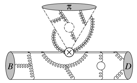
Figure 5: Collinear factorization of the $B\to D\pi$ decay in SCET.

Following the above explanation, the proof of the collinear factorization theorem for the decay $B\to D\pi$ in SCET is trivial [66]: the leading-power diagrams involve soft gluons exchanged among the quarks in the $B$ and $D$ mesons, and collinear gluons exchanged between the quarks in the pion. The former give the $B\to D$ form factor $F^{BD}$, defined as the matrix element of the frist piece of $O_{\bf\{0,8\}}$. The latter lead to the pion distribution amplitude $\phi_{\pi}(x)$, defined as the matrix element of the second piece with the Wilson coefficient $C_{\bf\{0,8\}}$ being excluded. The above discussion indicates that the pion distribution amplitude in Eq. (18) can be constructed in the framework of SCET. One simply identifies the correspondence of the quark fields $q$ in Eq. (18) and the collinear effective fields $\xi_{n,p}$ in Eq. (27), which are equivalent in the collinear region, and choose $\Gamma_{\ell}$ as $\gamma_{5}\not{\bar{n}}$. The two collinear Wilson lines $W$ correspond to the two pieces of path-ordered exponential in Eq. (18). The contributions from the diagrams in Fig. 2 are of the same power in $\lambda$ as of the effective current $\bar{\xi}_{n,p^{\prime}}^{(d)}W\Gamma_{\ell}W^{\dagger}\xi_{n,p}^{(u)}$ in Eq. (27).

Hence, only the diagrams of the type shown in Fig. 5 exist at leading power in SCET. The corresponding collinear factorization formula is then written as

$$\langle D^{(*)}\pi|H_{w}|B\rangle=N{F^{B\to D^{(*)}}(0)}\ \int_{0}^{1}dx\ {T(x,E,\mu)}\ {\phi_{\pi}(x,\mu)}+\cdots\,,$$ (29)

where $H_{w}$ is the weak effective Hamiltonian, $T(x,E,\mu)$ a calculable hard kernel, and the ellipses denote terms that vanish faster than the leading term as the pion energy $E\to\infty$. The dependences on the renormalization scale $\mu$ cancel between $T$ and $\phi_{\pi}$. The convolution in $x$ is a consequence of the non-commutative nature of the Wilson coefficients and the effective fields. The hard kernel can be determined by matching the effective theory to the full theory. Equation (29) was proposed in [68], proven to two-loops in [69], and proven to all orders in $\alpha_{s}$ in [66].

2.3 Jet Function

The application of collinear factorization theorem to exclusive $B$ meson decays has encountered a difficulty: the evaluation of the $B\to\pi$ transition form factors suffers the singularities from the end point of a momentum fraction $x\to 0$ [70, 71, 72]. These singularities are logarithmic and linear in the leading-twist (twist-2) and next-to-leading-twist (twist-3) contributions, respectively. On the other hand, the double logarithms $\alpha_{s}\ln^{2}x$ from radiative corrections were observed in the semileptonic decay $B\to\pi l\nu$ [73] and in the radiative decay $B\to\gamma l\nu$ [74]. It has been argued that when the end-point region is important, these double logarithms are not small expansion parameters, and should be organized into a quark jet function systematically in order to improve perturbative expansion. The procedure is referred to as threshold resummation [75]. The resultant Sudakov factor is found to vanish quickly as $x\to 0$. It turns out that in a self-consistent perturbative evaluation of the $B\to\pi$ form factors, where the original factorization formula is convoluted with the jet function, the end-point singularities do not exist [75].

I take the radiative decay $B\to\gamma l\nu$ as an example. The momentum $P_{1}$ of the $B$ meson and the momentum $P_{2}$ of the outgoing on-shell photon are parametrized as

$$P_{1}=\frac{m_{B}}{\sqrt{2}}(1,1,{\bf 0}_{T})\;,\;\;\;\;P_{2}=\frac{m_{B}}{\sqrt{2}}(0,\eta,{\bf 0}_{T})\;,$$ (30)

where $\eta$ denotes the energy fraction carried by the photon. Assume that the light spectator quark in the $B$ meson carries the momentum $k$. Consider the kinematic region with small $q^{2}$, $q=P_{1}-P_{2}$ being the lepton pair momentum, i.e., with large $\eta$, where perturbative expansion is reliable. The four components of the spectator quark momentum $k$ are of the same order as $\Lambda$. Here $\Lambda$ represents a hadronic scale, such as the $B$ meson and $b$ quark mass diffetrence, $m_{B}-m_{b}$. In collinear factorization, only the plus comonent $k^{+}$ is relevant through the inner product $k\cdot P_{2}$.

The lowest-order diagrams for the $B\to\gamma l\nu$ decay are displayed in Fig. 1, but with the upper quark (virtual photon) replaced by a $b$ quark ($W$ boson). It is easy to observe that Figs. 1(a) and 1(b) scale like $1/(\Lambda m_{B})$ and $1/m_{B}^{2}$, respectively, implying that Fig. 1(b) is power-suppressed. Below I will concentrate on Fig. 1(a). According to the leading-twist collinear factorization theorem discussed in Sec. 2.1, the $B\to\gamma l\nu$ decay amplitude is written as the convolution of a hard kernel $H(x,\eta,m_{B},\mu)$ with the $B$ meson distribution amplitude $\phi_{+}(x,\mu)$ over the parton momentum fraction $x=k^{+}/P_{1}^{+}$ [76],

$$A(\eta,m_{B})=\int dx\phi_{+}(x,\mu)H(x,\eta,m_{B},\mu)\;,$$ (31)

This expression has been derived in the framework of SCET [77, 78], in which the hard kernel was further factorized into $H=H_{h}H_{i}$ with the function $H_{h}$ and $H_{i}$ being characterized by the scale $m_{b}$ and $\sqrt{\Lambda m_{b}}$, respectively. Note that the jet function in [77, 78], referred to $H_{i}$, differs from that in [75].

Equation (31) is appropriate for the region with $k^{+}\sim O(\Lambda)$, in which the only infrared divergences are the soft ones absorbed into the $B$ meson distribution amplitude [50]. Near the end point $k^{+}\sim O(\Lambda^{2}/m_{B})$, the internal quark in Fig. 1(a) carries a large momentum $P_{2}-k$ with its invariant mass vanishing like $(P_{2}-k)^{2}=-2xP_{1}\cdot P_{2}\sim O(\Lambda^{2})$. This kinematics is similar to the threshold region of DIS with the Bjorken variable $x_{B}\to 1$, where the scattered quark also carries a large momentum and possesses a small invariant mass $(1-x_{B})s$, $s$ being the center-of-mass energy. In this region the scattered quark produces a jet of particles, to which the radiative corrections contain additional collinear divergences. Hence, a jet function needs to be introduced into the collinear factorization formula for DIS [79]. Similarly, a jet function has been incorporated into the factorization of direct photon production at a large photon transverse momentum (threshold) [80]. Here a jet function is associated with the internal quark near the end point of the momentum fraction involved in the decay $B\to\gamma l\nu$.

An additional collinear divergence from the loop momentum parallel to $P_{2}$ appears in the higher-order correction to the weak decay vertex shown in Fig. 2(d). This divergence can be extracted by replacing the $b$ quark line by an eikonal line in the direction of $n$. The factorization of the fermion flow is achieved by inserting the Fierz identity in Eq. (3), in which the first and last terms contribute in the combined structure $I_{ij}I_{lk}\to I_{ik}(\not n\not{\bar{n}})_{lj}/4$. Assigning the identity matrix $I$ to the trace for the hard kernel, one obtains Fig. 1(a). The matrix $\not n\not{\bar{n}}/4$ then leads to the loop integral [75],

$$J_{\parallel}^{(1)} = -ig^{2}C_{F}\int\frac{d^{4}l}{(2\pi)^{4}}\frac{1}{4}tr\left[\not n\not{\bar{n}}\gamma_{\beta}\frac{\not P_{2}-\not k+\not l}{(P_{2}-k+l)^{2}}\right]\frac{n^{\beta}}{n\cdot ll^{2}}\;,$$ (32)

$$= -\frac{\alpha_{s}}{4\pi}C_{F}\ln^{2}x+\cdots\;$$

which are the same as those derived in [74, 76, 78]. The correction to the photon vertex in Fig. 2(e) contains only the single logarithm $\alpha_{s}\ln x$, since the phase space of the loop momentum is restricted to $0<l^{+}<k^{+}\sim O(\Lambda^{2}/m_{B})$. The self-energy correction to the virtual light quark deos also. For the explicit expressions for the $O(\alpha_{s})$ corrections from Fig. 2, refer to [76].

The all-order factorization of the jet function from the decay $B\to\gamma l\nu$ has been proved following the procedure in Sec. 2.1, which provides a solid theoretical ground for the modified formalism appropriate for the end-point region. The jet function $J(x)$ is defined via

$$J(x)\bar{q}(P_{2}-k)\equiv\langle q(P_{2}-k)|{\bar{q}}(0)\frac{1}{4}\not n\not{\bar{n}}\exp\left[-ig\int_{-\infty}^{0}dzn\cdot A(zn)\right]|0\rangle\;.$$ (33)

The spinor $q(P_{2}-k)$ is associated with the internal quark, through which the momeutm $P_{2}-k$ flows. It is then understood from Eq. (33) that the jet function is universal.

I then discuss threshold resummation of the double logarithms $\alpha_{s}\ln^{2}x$ in the covariant gauge $\partial\cdot A=0$, which have been collected into the jet function to all orders. Threshold resummation for inclusive QCD processes has been studied intensively [81, 82]. Here I will adopt the framework developed in [83, 84], which has been shown to lead to the same results as in [81, 82]. First, allow the vector $n$ to contain a (small) minus component $n^{-}$. This modification, regularizing the collinear pole, extracts the double logarithm as shown in Eq. (32). The definition in Eq. (33) involves three variable vectors: the Wilson line direction $n$, the large momentum $P_{2}$, and the spectator momentum $k$. The scale invariance in $n$, as indicated by the Feynman rule associated with the eikonal line along $n$, implies that the jet function must depend on $k$ through the ratio $n\cdot k/n\cdot P_{2}$.

The next step is to derive the evolution of the jet function in $x$, i.e., in $k^{+}=xP_{1}^{+}$ by considering the derivative,

$$k^{+}\frac{dJ}{dk^{+}}=\frac{n\cdot k}{P_{2}\cdot k}P_{2}^{\alpha}\frac{dJ}{dn^{\alpha}}\;,$$ (34)

where the chain rule has been applied to relate the derivatives with respect to $k$ and to $n$. The differentiation $d/dn^{\alpha}$ operates on the eikonal line along $n$, giving

$$\frac{n\cdot k}{P_{2}\cdot k}P_{2}^{\alpha}\frac{d}{dn^{\alpha}}\frac{n_{\mu}}{n\cdot l}=\frac{{\hat{n}}_{\mu}}{n\cdot l}\;,\;\;\;\;{\hat{n}}_{\mu}=-\frac{n\cdot k}{P_{2}\cdot k}\frac{P_{2}\cdot l}{n\cdot l}n_{\mu}\;.$$ (35)

The loop momentum $l$ flowing through the special vertex does not generate a collinear divergence due to vanishing of the numerator $P_{2}\cdot l$ in the special vertex ${\hat{n}}_{\mu}$. It is easy to confirm that the ultraviolet region of $l$ does not produce $\ln x$ either. Therefore, one concentrates on the factorization of the soft gluon emitted from the special vertex, which can be achieved by applying the eikonal approximation to internal quark propagators, leading to ${\bar{n}}_{\nu}/{\bar{n}}\cdot l$. Following the reasoning in [84], the derivative of the jet function is written as

$$x\frac{dJ(x)}{dx}=-ig^{2}C_{F}\int\frac{d^{4}l}{(2\pi)^{4}}\frac{{\hat{n}}_{\mu}}{n\cdot l}\frac{g^{\mu\nu}}{l^{2}}\frac{{\bar{n}}_{\nu}}{{\bar{n}}\cdot l}J(x-l^{+}/P_{1}^{+})\;,$$ (36)

where the argument of $J$ in the integral arises from the invariant mass of the internal quark, $(P_{2}-k+l)^{2}\approx-2(x-l^{+}/P_{1}^{+})P_{1}\cdot P_{2}$. The integrand corresponds to the diagram with the soft gluon attaching the eikonal lines along $n$ and along $\bar{n}$. Performing the integration over $l^{-}$ and $l_{T}$, one derives the evolution equation,

$$x\frac{dJ(x)}{dx}=\frac{\alpha_{s}}{2\pi}C_{F}\int_{x}^{1}\frac{d\xi}{(\xi-x)_{+}}J(\xi)\;,$$ (37)

where the variable change from $l^{+}$ to $\xi$ has been made. The plus distribution is defined such that, when $1/(\xi-x)_{+}$ is integrated with a function $f(\xi)$, one must replace it by $f(\xi)-f(x)$ in the integral. It has been shown that the above evolution equation is similar to that for unintegrated parton distribution functions involved in inclusive QCD processes [85], which resums the same double logarithm $\alpha_{s}\ln^{2}x$.

The analytical solution is a Sudakov factor,

$$J(x)=-\exp\left(\frac{\pi^{2}}{4}\gamma_{K}\right)\int_{-\infty}^{\infty}\frac{dt}{\pi}(1-x)^{\exp(t)}\sin\left(\frac{\pi}{2}\gamma_{K}t\right)\exp\left(-\frac{1}{4}\gamma_{K}t^{2}\right)\;,$$ (38)

with the anomalous dimension $\gamma_{K}=\alpha_{s}C_{F}/\pi$. It is trivial to check that $J(x)$ is normalized to unity, $\int J(x)dx={\tilde{J}}(1)=1$ [86]. Obviously, Eq. (38) vanishes at $x\to 0$, because the integrand is an odd function in $t$, and at $x\to 1$ due to the factor $(1-x)^{\exp(t)}$. Moreover, Eq. (38) provides suppression near the end point $x\to 0$, which is stronger than any power of $x$. This is understood from vanishing of all the derivatives of Eq. (38) with respect to $x$ at $x\to 0$ [75]. To the accuracy of the next-to-leading logarithms, the running of the coupling constant $\alpha_{s}$ should be taken into account, and Eq. (38) will be modified. However, the above features remain.

I emphasize the differences among the Sudakov resummations for the $B\to\gamma l\nu$ decay in the literature. In [74] it is the double logarithm $\ln^{2}(k_{T}/m_{B})$ that was resummed. In [76] it is the double logarithm $\ln^{2}(E_{\gamma}/m_{B})$, $E_{\gamma}$ being the photon energy, that was resummed. In [78] the evolution from the scale of $O(\sqrt{\Lambda m_{b}})$ to the scale of $O(m_{b})$ was derived by solving the renormalization-group equations,

$$\frac{d}{d\ln\mu}\,H_{h}(\mu) = \left[-\Gamma_{\rm cusp}(\alpha_{s})\,\ln\frac{\mu}{2E_{\gamma}}+\gamma(\alpha_{s})-\gamma^{\prime}(\alpha_{s})\right]H_{h}(\mu)\,,$$ (39)

$$\frac{d}{d\ln\mu}\,H_{i}(l_{+},\mu) = \left[\Gamma_{\rm cusp}(\alpha_{s})\,\ln\frac{\mu^{2}}{2E_{\gamma}\,l_{+}}+\gamma^{\prime}(\alpha_{s})\right]H_{i}(l_{+},\mu)+\int_{0}^{\infty}\!d\omega\,\Gamma(\omega,l_{+},\alpha_{s})\,H_{i}(\omega,\mu)\,.$$ (40)

$\Gamma_{\rm cusp}$ is the universal cusp anomalous dimension familiar from the theory of the renormalization of Wilson loops [87]. The anomalous dimensions $\gamma$ and $\gamma^{\prime}$ are given by [78]

$$\gamma(\alpha_{s})=-2C_{F}\,\frac{\alpha_{s}}{4\pi}+O(\alpha_{s}^{2})\,,\qquad\gamma^{\prime}(\alpha_{s})=O(\alpha_{s}^{2})\,.$$ (41)

The function $\Gamma$ obeys $\int d\omega\,\Gamma(\omega,\omega^{\prime},\alpha_{s})=0$, whose one-loop expression is written as

$$\Gamma^{\rm 1-loop}(\omega,\omega^{\prime},\alpha_{s})=-\Gamma_{\rm cusp}^{\rm 1-loop}(\alpha_{s})\left[\frac{\omega^{\prime}}{\omega}\,\frac{\theta(\omega-\omega^{\prime})}{\omega-\omega^{\prime}}+\frac{\theta(\omega^{\prime}-\omega)}{\omega^{\prime}-\omega}\right]_{+}\;.$$ (42)

It was found that the resummation effect decreases the magnitude of the radiative corrections, i.e., the renormalization-group improved kernel is closer to the tree-level value than the one-loop result [78].

The formalism for threshold resummation has been extended to the semileptonic decay $B\to\pi l\nu$ in the fast recoil region of the pion. The $B$ meson momentum $P_{1}$ is the same as in the decay $B\to\gamma l\nu$, and the pion momentum $P_{2}$ is the same as the photon momentum. Leading-twist factorization theorem for the $B\to\pi$ form factor $F(q^{2})$ has been proved in [50],

$$F(q^{2})=\sum_{m=+,-}\int_{0}^{1}dx_{1}dx_{2}\phi_{m}(x_{1}){\cal H}_{m}(x_{1},x_{2},\eta)\phi_{\pi}(x_{2})\;,$$ (43)

which holds in the region with $x_{1}\sim O(\Lambda/m_{B})$ and with $x_{2}\sim O(1)$. The light-cone $B$ meson distribution amplitudes $\phi_{m}$ will be defined in the next section.

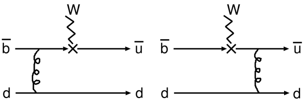
Figure 6: Leading-order contribution to $F^{B\pi}$.

Since Fig. 6(a), proportional to $1/(x_{1}x_{2}^{2})$, is more singular at small $x_{2}$, one considers the end-point region with $x_{2}\sim O(\Lambda/m_{B})$, where the internal $b$ quark propagator scales like $1/({\Lambda}m_{B})$. The loop correction to the weak vertex, where the radiative gluon attaches the virtual $b$ quark and upper valence quark in the pion, generates the double logarithm $\alpha_{s}\ln^{2}x_{2}$ from the collinear region with the loop momentum parallel to $P_{2}$. This double logarithm, similar to that in Eq. (32), is grouped into a jet funciton. It is easy to show that this jet function obeys the evolution equation in Eq. (37). Hence, the threshold resummation leads to a result the same as Eq. (38). That is, the Sudakov factor is universal. The analysis for Fig. 6(b) is similar to that for the decay $B\to\gamma l\nu$. In the end-point region with $x_{1}\sim O(\Lambda^{2}/m_{B}^{2})$, additional collinear divergences associated with the internal light quark are produced. The loop correction to the weak vertex, where the radiative gluon attaches the $b$ quark and the virtual light quark, gives the double logarithm $\alpha_{s}\ln^{2}x_{1}$, whose factorization is the same as of Fig. 2(d).

The modified collinear factorization formula appropriate for the end-point region is then written as

$$F(q^{2})=\sum_{m=+,-}\sum_{i=1,2}\int_{0}^{1}dx_{1}dx_{2}\phi_{m}(x_{1})H_{m}^{(i)}(x_{1},x_{2},\eta)J(x_{i})\phi_{\pi}(x_{2})\;,$$ (44)

with the index $i=1$ (2) corresponding to Fig. 6(b) [(a)]. If $J(x)$ is excluded, the above expression is divergent because of $H_{m}^{(2)}\propto 1/x_{2}^{2}$ and $\phi_{\pi}\propto x_{2}$ at $x_{2}\to 0$. Including the threshold resummation, the $B\to\pi$ form factor is calculable without introducing any infrared cutoffs [70, 72]. The numerical effect from the jet function on the $B\to\pi$ form factor has been examined in [75].

In a recent work based on SCET, a jet function has also been defined in the analysis of the decay $B\to\pi l\nu$ [88]. It was also concluded that the end-point singularity does not exist in the $B\to\pi$ transiton form factors in the convolution with the jet function. I stress that the jet function in [88] differs from the one considered here, and that the smearing mechanism of the end-point singularity is also different: it is not attributed to the Sudakov mechanism discussed above. The jet function in [88], absorbing dynamics characterized by $O(\sqrt{\Lambda m_{B}})$, more or less corresponds to the finite piece of the hard kernels in collinear factorization theorem without threshold resummation. In the case of the $B\to\pi$ transiton form factors, it can be identified as the piece from Fig. 6(a), which is proportional to $1/x_{2}$. This piece is free of the end-point singularity, nothing to do with the Sudakov effect. This point will be elucidated in detail in Sec. 4.3.

3 $k_{T}$ Factorization

Both collinear and $k_{T}$ factorizations are the fundamental tools of QCD perturbation theory, where $k_{T}$ denotes parton transverse momenta. For inclusive processes, consider DIS of a hadron, carrying a momentum $p$, by a virtual photon, carrying a momentum $q$. Collinear factorization [89] and $k_{T}$ factorization [90, 91, 92] apply, when DIS is measured at a large and small Bjorken variable $x_{B}\equiv-q^{2}/(2p\cdot q)$, respectively. The cross section is written as the convolution of a hard subprocess with a hadron distribution function in a parton momentum fraction $x$ in the former, and in both $x$ and $k_{T}$ in the latter. When $x_{B}$ is small, $x\geq x_{B}$ can reach a small value, at which $k_{T}$ is of the same order of magnitude as the longitudinal momentum $xp$, and not negligible. For exclusive processes, such as hadron form factors, collinear factorization was developed in [43, 44, 45, 46, 47, 48] as stated in the previous section. The range of a parton momentum fraction $x$, contrary to that in the inclusive case, is not experimentally controllable, and must be integrated over between 0 and 1. Hence, the end-point region with a small $x$ is not avoidable. If no end-point singularity is developed, collinear factorization works. If such a singularity occurs, indicating the breakdown of collinear factorization, $k_{T}$ factorization should be employed. In fact, the recent observation $QF_{2}(Q^{2})/F_{1}(Q^{2})\sim$ const. [93], $F_{1}$ and $F_{2}$ being the proton Dirac and Pauli form factors, respectively, indicates that $k_{T}$ factorization is the appropriate tool for studying exclusive processes [94]. Since $k_{T}$ factorization theorem was proposed [95, 96], there had been wide applications to various processes [97].

In this section I review $k_{T}$ factorization theorem for exclusive processes. It is more convenient to perform $k_{T}$ factorization in the impact parameter $b$ space, in which infrared divergences in radiative corrections can be extracted from parton-level diagrams explicitly. The procedure is basically similar to that for collinear factorization in Sec. 2.1, if the proof is performed in the impact parameter $b$ space. It has been observed that collinear factorization is the $b\to 0$ limit of $k_{T}$ factorization. I explain how to construct a gauge-invariant $b$-dependent meson wave function defined as a nonlocal matrix element with a special path for the Wilson line. The application of $k_{T}$ factorization theorem to exclusive $B$ meson decays, and the behavior of $b$-dependent $B$ meson wave functions are discussed. Retaining the parton transverse degrees of freedom, the double logarithms $\alpha_{s}\ln^{2}k_{T}$ appear, which should be organized to all orders. The basic idea for $k_{T}$ resummation of these double logarithms into a Sudakov factor [24] is given. The end-point singularity in the heavy-to-light transition form factors can also be smeared [24, 25, 26, 98, 99] by including this Sudakov factor.

3.1 Gauge Invariance

I again start with the process $\pi\gamma^{\ast}\to\gamma$ [100]. This process, though containing no end-point singularity, is simple and appropriate for a demonstration. The momentum $P_{1}\;(P_{2})$ of the initial-state pion (final-state photon) is chosen as in Eq. (1). I explain how to perform the factorization of the collinear enhancement from $l$ parallel to $P_{1}$ without integrating out the transverse components $l_{T}$. The lowest-order diagrams are displayed in Fig. 1, and the $O(\alpha_{s}^{0})$ $k_{T}$ factorization formula is the same as the collinear factorization formula in Eq. (4). That is, none of ${\cal G}^{(0)}$, $\phi^{(0)}$, and ${\cal H}^{(0)}$ depends on a transverse momentum. The wave function and the hard kernel become $l_{T}$-dependent through collinear gluon exchanges at higher orders.

The $O(\alpha_{s})$ $k_{T}$ factorization formula is a sum over the diagrams in Fig. 2, the same as Eq. (7), but with each term being written as the convolution in the momentum fraction $\xi$ and in the impact parameter $b$,

$${\cal G}^{(1)}_{i}(x) = \int d\xi\frac{d^{2}b}{(2\pi)^{2}}\Phi_{i}^{(1)}(x,\xi,b)H^{(0)}(\xi,b)+\phi^{(0)}(x){\cal H}_{i}^{(1)}(x)\;.$$ (45)

The above expression, with the $O(\alpha_{s})$ wave functions $\Phi_{i}^{(1)}(x,\xi,b)$ and $H^{(0)}(\xi,b)$ specified, defines the $O(\alpha_{s})$ hard kernels ${\cal H}_{i}^{(1)}(x)$, which do not contain collinear divergences. Equation (45) is a consequence of the assertion that partons acquire transverse degrees of freedom through collinear gluon exchanges: ${\cal H}^{(1)}$, convoluted with the lowest-order $l_{T}$-independent $\phi^{(0)}$, is then identical to that in collinear factorization. As shown later, this consequence is crucial for constructing gauge-invariant hard kernels.

The $O(\alpha_{s})$ wave functions obtained from Figs. 2(a) and 2(c) are the same as in collinear factorization. The $k_{T}$ factorization of Fig. 2(b) leads to the wave function,

$$\Phi^{(1)}_{b}(x,\xi,b) = \frac{ig^{2}C_{F}}{4P_{1}^{+}}\int\frac{d^{4}l}{(2\pi)^{4}}{\bar{q}}(xP_{1})\frac{\gamma^{\nu}(x\not P_{1}-\not l)\gamma^{5}\not{\bar{n}}({\bar{x}}\not P_{1}+\not l)\gamma_{\nu}}{(xP_{1}-l)^{2}({\bar{x}}P_{1}+l)^{2}l^{2}}q({\bar{x}}P_{1})$$ (46)

$$\times\delta\left(\xi-x+\frac{l^{+}}{P_{1}^{+}}\right)e^{-i{\bf l}_{T}\cdot{\bf b}}\;.$$

The Fourier transformation introduces the additional factor $\exp(-i{\bf l}_{T}\cdot{\bf b})$ into the wave function $\Phi^{(1)}_{b}$ compared to the result in collinear factorization in Eq. (8), since the hard kernel depends on $l_{T}$ in this case. The $O(\alpha_{s})$ wave function extracted from Fig. 2(d) is written as

$$\Phi^{(1)}_{d}(x,\xi,b) = \frac{-ig^{2}C_{F}}{4P_{1}^{+}}\int\frac{d^{4}l}{(2\pi)^{4}}{\bar{q}}(xP_{1})\gamma^{5}\not{\bar{n}}\frac{{\bar{x}}\not P_{1}+\not l}{({\bar{x}}P_{1}+l)^{2}}\gamma_{\nu}q({\bar{x}}P_{1})\frac{1}{l^{2}}\frac{{\bar{n}}^{\nu}}{{\bar{n}}\cdot l}$$ (47)

$$\times\left[\delta(\xi-x)-\delta\left(\xi-x+\frac{l^{+}}{P_{1}^{+}}\right)e^{-i{\bf l}_{T}\cdot{\bf b}}\right]\;.$$

The second term acquires the additional factor $\exp(-i{\bf l}_{T}\cdot{\bf b})$ from the Fourier transformation, because it corresponds to the case with the loop momentum $l$ flowing through the hard kernel. It is easy to observe that the soft divergences cancel among the $O(\alpha_{s})$ radiative corrections: in the soft region of $l$ we have $\exp(-i{\bf l}_{T}\cdot{\bf b})\approx 1$ and $l^{+}\approx 0$, and the two terms in Eq. (47) cancel. Similarly, the soft divergences cancel among Figs. 2(a)-2(c).

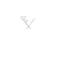
Figure 7: The special path for the Wilson line in a $b$-dependent wave function.

One constructs the parton-level wave function as the nonlocal matrix element in the $b$ space,

$$\Phi(x,\xi,b)=i\int\frac{dy^{-}}{2\pi}e^{-i\xi P_{1}^{+}y^{-}}\langle 0|{\bar{q}}(y)\gamma_{5}\not{\bar{n}}P\exp\left[-ig\int_{0}^{y}ds\cdot A(s)\right]q(0)|{\bar{q}}(xP_{1})q({\bar{x}}P_{1})\rangle\;,$$ (48)

with the coordinate $y=(0,y^{-},{\bf b})$. The path for the Wilson line is composed of three pieces: from 0 to $\infty$ along the direction of ${\bar{n}}$, from $\infty$ to $\infty+{\bf b}$, and from $\infty+{\bf b}$ back to $y$ along the direction of $-{\bar{n}}$ as displayed in Fig. 7. The first (third) piece corresponds to the eikonal line associated with the first (second) term in Eq. (47).

For the evaluation of the lowest-order hard kernel, one neglects only the minus component $l^{-}$ in the denominator [see the second term on the right-hand side of Eq. (10)],

$$(P_{2}-xP_{1}+l)^{2}\approx-(2\xi P_{1}\cdot P_{2}+l_{T}^{2})\;.$$ (49)

Note that in collinear factorization both $l^{-}$ and $l_{T}$ are dropped. The $b$-dependent hard amplitude is then given by,

$$H^{(0)}(\xi,b) = \int d^{2}l_{T}{\cal H}^{(0)}(\xi,l_{T})\exp(i{\bf l}_{T}\cdot{\bf b})\;,$$

$${\cal H}^{(0)}(\xi,l_{T}) = ie^{2}\frac{tr(\not\epsilon\not P_{2}\gamma_{\mu}\not P_{1}\gamma^{5})}{2\xi P_{1}\cdot P_{2}+l_{T}^{2}}\;.$$ (50)

Equivalently, the above ${\cal H}^{(0)}(\xi,l_{T})$ is derived by considering an off-shell $\bar{q}$ quark, which carries the momentum $\xi P_{1}-{\bf l}_{T}$, and the leading structure $\not P_{1}\gamma_{5}$ associated with the pion, which is the same as in collinear factorization.

I now demonstrate the gauge invariance of $k_{T}$ factorization theorem. Equation (48) is explicitly gauge-invariant because of the presence of the Wilson link from $0$ to $y$ [91, 101]. ${\cal H}^{(1)}(x)$, the same as in collinear factorization, is gauge-invariant. From Eq. (45), the gauge invariance of $\Phi^{(1)}(x,\xi,b)$ stated above, together with the gauge invariance of ${\cal G}^{(1)}(x)$ and ${\cal H}^{(1)}(x)$, then imply the gauge invariance of $H^{(0)}(\xi,b)$. Similarly, the $k_{T}$ factorization formula of $O(\alpha_{s}^{2})$,

$${\cal G}^{(2)}(x)=\int d\xi\frac{d^{2}b}{(2\pi)^{2}}\left[\Phi^{(2)}(x,\xi,b)H^{(0)}(\xi,b)+\Phi^{(1)}(x,\xi,b)H^{(1)}(\xi,b)\right]+\phi^{(0)}(x){\cal H}^{(2)}(x)\;,$$ (51)

leads to the gauge invariance of $H^{(1)}(\xi,b)$. Therefore, the hard kernels in $k_{T}$ factorization are gauge-invariant at all orders.

After determining the gauge-invariant infrared-finite hard kernel $H$, one convolutes it with the physical two-parton pion wave function, whose all-order gauge-invariant definition is written as

$$\Phi_{\pi}(x,b,Q,\mu)=i\int\frac{dy^{-}}{2\pi}e^{-ixP_{1}^{+}y^{-}}\langle 0|{\bar{q}}(y)\gamma_{5}\not{\bar{n}}{\cal P}\exp\left[-ig\int_{0}^{y}ds\cdot A(s)\right]q(0)|\pi(P_{1})\rangle\;.$$ (52)

The relevant form factor $F(Q^{2})$ for the process $\pi\gamma^{*}\to\gamma$ is then expressed as

$$F(Q^{2})=\int_{0}^{1}dx\int\frac{d^{2}b}{(2\pi)^{2}}\Phi_{\pi}(x,b,Q,\mu)H(x,b,Q,\mu)\;.$$ (53)

where both the dependences on $Q$ and on the factorization scale $\mu$ have been made explicit. It has been concluded that predictions derived from $k_{T}$ factorization theorem are gauge-invariant and infrared-finite [102].

In summary, a two-parton $b$-dependent wave function is factorized from parton-level diagrams in a way the same as in collinear factorization (for example, under the same eikonal approximation), but the loop integrand is associated with an additional Fourier factor $\exp(-i{\bf l}_{T}\cdot{\bf b})$, when the loop momentum $l$ flows through a hard kernel. A $k_{T}$-dependent hard kernel is obtained in a way the same as in collinear factorization, but considering off-shell external partons, which carry the fractional momenta $k=xP-{\bf k}_{T}$ ($k^{2}=-k_{T}^{2}$), $P$ being the external meson momenta. Then Fourier transform this hard kernel into the $b$ space. The insertion of the Fierz identity to separate the fermion flow between a wave function and a hard amplitude is the same as in collinear factorization. For inclusive processes in small $x_{B}$ physics, the gauge invariance of the unintegrated gluon distribution function and of the hard subprocess of reggeized gluons, being also off-shell by $-k_{T}^{2}$, is ensured in a similar way. The distinction is that the structures of $\gamma$-matrices from the Fierz identity are replaced by eikonal vertices, which contain only the longitudinal components [91].

3.2 $B$ Meson Wave Functions

In this subsection I review the $k_{T}$ factorization theorem for exclusive $B$ meson decays by considering the radiative decay $B\to\gamma l\nu$. It has been shown that in heavy quark limit a gauge-invariant $b$-dependent $B$ meson wave function can be defined, which absorbs soft divergences in the decay process, differing from the collinear divergences in the pion wave function. As explained below, exclusive $B$ meson decays are characterized by the scale $\sqrt{\Lambda m_{B}}$. In terms of the power counting in SCET, the soft dynamics discussed here is referred to as the usoft one, since the typical momentum behaves like [50]

$$l^{\mu}\sim(\Lambda,\Lambda,\Lambda)\sim m_{B}(\lambda^{2},\lambda^{2},\lambda^{2})\;,$$ (54)

for the expansion parameter $\lambda\sim\sqrt{\Lambda/m_{B}}$. It is possible to construct a light-cone $B$ meson wave function, if an appropriate frame with the photon moving along the light cone is chosen.

Figure 1(a) gives the parton-level amplitude,

$${\cal G}^{(0)}(x) = e{\bar{q}}(k)\not\epsilon\frac{\not P_{2}-\not k}{(P_{2}-k)^{2}}\gamma_{\mu}(1-\gamma_{5})b(P_{1}-k)\;,$$ (55)

which does not depend on a transverse momentum. Inserting the Fierz identity in Eq. (3) into Eq. (55), one obtains Eq. (4) with

$$\phi^{(0)}(x) = \frac{1}{4P_{1}^{+}}{\bar{q}}(k)\gamma_{5}\not{\bar{n}}b(P_{1}-k)\;,$$

$${\cal H}^{(0)}(x) = -e\frac{tr[\not\epsilon\not P_{2}\gamma_{\mu}(1-\gamma_{5})(\not P_{1}+m_{B})(\not n/\sqrt{2})\gamma^{5}]}{2xP_{1}\cdot P_{2}}\;,$$ (56)

where the higher-power term $\not k$ in the numerator has been dropped. For the $B$ meson, there are two leading-twist wave functions associated with the structures $\gamma_{5}\gamma^{\pm}$. For the $B\to\gamma l\nu$ decay, only the structure $\gamma_{5}\gamma^{+}=\gamma_{5}\not{\bar{n}}$ contributes: since $\not\epsilon$ in Eq. (56) involves $\gamma_{T}$, only the structure $\gamma^{-}\gamma_{5}=\not n\gamma_{5}$ contributes to the hard kernel.

Next one considers the $O(\alpha_{s})$ radiative corrections to Fig. 1(a) shown in Fig. 2, and discuss the factorization of the soft divergence from the region of the loop momentum in Eq. (54). The dependence of the $B$ meson wave function on the transverse momentum is generated by soft gluon exchanges. The analysis is similar to that in Sec. 3.1, and one derives Eq. (45). The factorization of the two-particle reducible diagrams in Fig. 2(a)-2(c) is straightforward. Take Fig. 2(b) as an example. Employing the eikonal approximation in the heavy quark limit, one has

$$\frac{\not P_{1}-\not k+\not l+m_{b}}{(P_{1}-k+l)^{2}-m_{b}^{2}}\gamma_{\nu}b(P_{1}-k)\approx\frac{v_{\nu}}{v\cdot l}b(P_{1}-k)\;,$$ (57)

with the velocity $v=P_{1}/m_{B}$. The $O(\alpha_{s})$ wave function extracted from Fig. 2(b) is then written as

$$\Phi^{(1)}_{b}(x,\xi,b) = \frac{ig^{2}C_{F}}{4P_{1}^{+}}\int\frac{d^{4}l}{(2\pi)^{4}}{\bar{q}}(k)\frac{\gamma^{\nu}(\not k-\not l)}{(k-l)^{2}l^{2}}\gamma_{5}\not{\bar{n}}b(P_{1}-k)\frac{v_{\nu}}{v\cdot l}\delta\left(\xi-x+\frac{l^{+}}{P_{1}^{+}}\right)e^{-i{\bf l}_{T}\cdot{\bf b}}\;.$$ (58)

Performing the contour integration over, say, $l^{-}$, one observes that the integral is singular only when the component $l^{+}$ is of $O(\Lambda)$. This observation implies that the infrared divergence associated with the $B$ meson is of the soft type, and that $l^{+}$, being of the same order of magnitude as $k^{+}=xP_{1}^{+}$, is not negligible in the $\delta$-function. Therefore, the soft divergences in Figs. 2(a)-2(c) do not cancel in $B$ meson decays [24]. The explanation is simple: the light spectator quark, carrying a small amount of momenta, forms a color cloud around the $b$ quark. This cloud is also huge in space-time, such that soft gluons resolve the color structure of the $B$ meson.

Diagrams with the radiative gluon attaching the internal quark in Figs. 2(d) and 2(e) also contain soft divergences, because the internal quark is off-shell by $O(\Lambda m_{B})$, which defines the characteristic scale of the decay $B\to\gamma l\nu$. Note that the internal quark in the process $\pi\gamma^{*}\to\gamma$ is off-shell by $O(Q^{2})$. One extracts the $O(\alpha_{s})$ wave function from Fig. 2(d),

$$\Phi^{(1)}_{d}(x,\xi,b) = \frac{-ig^{2}C_{F}}{4P_{1}^{+}}\int\frac{d^{4}l}{(2\pi)^{4}}{\bar{q}}(xP_{1})\gamma_{5}\not{\bar{n}}b(P_{1}-k)\frac{1}{l^{2}}\frac{{\bar{n}}\cdot v}{{\bar{n}}\cdot lv\cdot l}$$ (59)

$$\times\left[\delta(\xi-x)-\delta\left(\xi-x+\frac{l^{+}}{P_{1}^{+}}\right)e^{-i{\bf l}_{T}\cdot{\bf b}}\right]\;.$$

The eikonal approximation in Eq. (57) has been applied. The above expression implies that the infrared divergences in the irreducible diagrams can also be collected by the eikonal line along the light cone. This is attributed to the choice of the frame, in which the photon moves in the minus direction.

Following the procedure in Sec. 3.1, one constructs a gauge-invariant light-cone $B$ meson wave function,

$$\Phi_{+}(x,b,m_{B},\mu) = i\int\frac{dy^{-}}{2\pi}e^{-ixP_{1}^{+}y^{-}}\langle 0|{\bar{q}}(y)\gamma_{5}\gamma^{+}{\cal P}\exp\left[-ig\int_{0}^{y}ds\cdot A(s)\right]b_{v}(0)|B(P_{1})\rangle\;,$$ (60)

where $b_{v}$ is the rescaled $b$ quark field, and the decay constant $f_{B}$ has been omitted. The Feynman rules associated with $b_{v}$ are those for an eikonal line in the direction of $v$ defined in Eq. (57). The lowest-order hard kernel in the $b$ space is given by Eq. (50) with

$${\cal H}^{(0)}(\xi,l_{T}) = -e\frac{tr[\not\epsilon\not P_{2}\gamma_{\mu}(1-\gamma_{5})(\not P_{1}+m_{B})(\not n/\sqrt{2})\gamma^{5}]}{2\xi P_{1}\cdot P_{2}+l_{T}^{2}}\;,$$ (61)

$\xi=(k^{+}-l^{+})/P_{1}^{+}$ being the momentum fraction. The above expression can be derived by considering an off-shell $\bar{q}$ quark of the momentum $(\xi P_{1}^{+},0,-{\bf l}_{T})$, and by contracting the parton-level diagram with the leading structure $(\not P_{1}+m_{B})(\not n/\sqrt{2})\gamma^{5}$, which is the same as in collinear factorization.

The semileptonic decay $B\to\pi l\nu$, because of the end-point singularity, demands $k_{T}$ factorization, whose all-order proof can be performed in a similar way. For this mode, both the leading-twsit $B$ meson wave functions $\phi_{\pm}$, associated with the structures $\gamma_{5}\gamma^{\pm}$, contribute [50]. Moreover, contributions from the pseudo-scalar and pseudo-tensor two-parton twist-3 pion distribution amplitudes are also leading-power [98]. The factorization of the corresponding collinear divergences has been proved [50]. The point is to replace the Dirac structure $\gamma_{5}\gamma^{\alpha}$ by the corresponding ones $\gamma_{5}$ and $\gamma_{5}\sigma^{\alpha\beta}$ in Eq. (3).

I then discuss the behavior of the $B$ meson wave functions constructed in Eq. (60). In the heavy quark limit the two-parton light-cone wave functions $\tilde{\Phi}_{\pm}(t,z^{2})$ are defined in terms of the nonlocal matrix element [103, 104]:

$$\langle 0|\bar{q}(y)\Gamma b_{v}(0)|\bar{B}(P_{1})\rangle=-\frac{if_{B}m_{B}}{2}tr\left[\gamma_{5}\Gamma\frac{1+\not{v}}{2}\left\{\tilde{\Phi}_{+}(t,y^{2})-\not{y}\frac{\tilde{\Phi}_{+}(t,y^{2})-\tilde{\Phi}_{-}(t,y^{2})}{2t}\right\}\right]\;,$$ (62)

with $t=v\cdot y$, $y^{2}=-b^{2}$, and $\Gamma$ being a Dirac matrix .

Consider the light-cone distribution amplitudes in terms of the variable $\omega=xm_{B}$ [103],

$$\phi_{\pm}(\omega)=\lim_{y^{2}\to 0}\Phi_{\pm}(\omega,y^{2})\;,$$ (63)

where the wave functions $\Phi_{\pm}(\omega,y^{2})$, defined in Eq. (60), come from the Fourier transformation of $\tilde{\Phi}_{\pm}(t,y^{2})$. The differential equations are written as [105]

$$\omega\frac{d\phi_{-}(\omega)}{d\omega} + \phi_{+}(\omega)=I(\omega)\ ,$$

$$\left(\omega-2\Lambda\right)\phi_{+}(\omega) + \omega\phi_{-}(\omega)=J(\omega)\ ,$$ (64)

where $I(\omega)$ and $J(\omega)$ denote the source terms due to three-parton wave functions $\Psi_{A}$, $\Psi_{V}$ and $X_{A}$:

$$I(\omega) = 2\frac{d}{d\omega}\int_{0}^{\omega}d\rho\int_{\omega-\rho}^{\infty}\frac{d\xi}{\xi}\frac{\partial}{\partial\xi}\left[\Psi_{A}(\rho,\xi)-\Psi_{V}(\rho,\xi)\right]\;,$$

$$J(\omega) = -2\frac{d}{d\omega}\int_{0}^{\omega}d\rho\int_{\omega-\rho}^{\infty}\frac{d\xi}{\xi}\left[\Psi_{A}(\rho,\xi)+X_{A}(\rho,\xi)\right]-4\int_{0}^{\omega}d\rho\int_{\omega-\rho}^{\infty}\frac{d\xi}{\xi}\frac{\partial\Psi_{V}(\rho,\xi)}{\partial\xi}\;.$$ (65)

The solution can be decomposed into two pieces:

$$\phi_{\pm}(\omega)=\phi_{\pm}^{(W)}(\omega)+\phi_{\pm}^{(g)}(\omega)\;.$$ (66)

The functions $\phi_{\pm}^{(W)}(\omega)$ are the solution with $I(\omega)=J(\omega)=0$, corresponding to the “Wandzura-Wilczek approximation” [106, 107] $\Psi_{V}=\Psi_{A}=X_{A}=0$. The functions $\phi_{\pm}^{(g)}(\omega)$ are induced by the source terms $I(\omega)$ and $J(\omega)$. The analytic expressions for the Wandzura-Wilczek part are given by

$$\phi_{\pm}^{(W)}(\omega)=\frac{\Lambda\pm(\omega-\Lambda)}{2\Lambda^{2}}\theta(\omega)\theta(2\Lambda-\omega)\;.$$ (67)

The expressions for $\phi_{\pm}^{(g)}$, in terms of $\Psi_{A}$, $\Psi_{V}$ and $X_{A}$, can be found in [108]. Equation (67) is quite different from the model distribution amplitudes appearing in the literature. One example of such models is [103]

$$\phi^{GN}_{+}(\omega) = \frac{\omega}{\omega_{0}^{2}}\exp\left(-\frac{\omega}{\omega_{0}}\right)\;,$$

$$\phi^{GN}_{-}(\omega) = \frac{1}{\omega_{0}}\exp\left(-\frac{\omega}{\omega_{0}}\right)\;,$$ (68)

with $\omega_{0}=2\Lambda/3$, which are inspired by the QCD sum rule estimates [103]. Note that, however, the behavior $\phi_{+}^{GN}(\omega)\sim\omega$ and $\phi_{-}^{GN}(\omega)\sim{\rm constant}$ at $\omega\rightarrow 0$ is consistent with Eq. (67). Another example comes from solving an integro-differential equation [109]: evolution effects generate a radiative tail, which falls off slower than $1/\omega$.

Including the $k_{T}$ (or $y^{2}=-b^{2}$) dependence, one has the differential equations [108]

$$\omega\frac{\partial\Phi_{-}}{\partial\omega}+\Phi_{+}+z^{2}\frac{\partial}{\partial z^{2}}\left(\Phi_{+}-\Phi_{-}\right)=0\;,$$

$$\left(\omega\frac{\partial}{\partial\omega}+2\right)\left(\Phi_{+}-\Phi_{-}\right)+4\frac{\partial^{2}}{\partial\omega^{2}}\frac{\partial\Phi_{+}}{\partial z^{2}}=0\;,$$

$$\left[(\omega-\Lambda)\frac{\partial}{\partial\omega}\!+\!\frac{3}{2}\right]\Phi_{+}\!-\!\frac{1}{2}\Phi_{-}\!+2\frac{\partial^{2}}{\partial\omega^{2}}\frac{\partial\Phi_{+}}{\partial z^{2}}\!=0\;,$$

$$\left[(\omega-\Lambda)\frac{\partial}{\partial\omega}+2\right]\left(\Phi_{+}-\Phi_{-}\right)+2\frac{\partial^{2}}{\partial\omega^{2}}\left(\frac{\partial\Phi_{+}}{\partial z^{2}}-\frac{\partial\Phi_{-}}{\partial z^{2}}\right)=0\;.$$ (69)

The solution in the Wandzura-Wilczek approximation is given by

$$\Phi^{(W)}_{\pm}(\omega,b)\sim\frac{1}{\sqrt{b}}\cos\left(\sqrt{\omega(2\Lambda-\omega)}\;b-\frac{\pi}{4}\right)\;,$$ (70)

where the $b$ dependence corresponds to $\delta(k_{T}^{2}-\omega(2\Lambda-\omega))$ in $k_{T}$ space. It is observed that the longitudinal and transverse momentum dependences do not seperate (factorize) in Eq. (70), contrary to the assumption in many models [25, 104, 110]. The Gaussian distribution for the $k_{T}$-dependence has been adopted in [25], which exhibits strong damping at large $b$ as $\exp\left(-\omega_{B}^{2}b^{2}/2\right)$ (see Sec. 4.3). In contrast, the results in Eq. (70) show slow-damping with oscillatory behavior. I mention that, despite of the different functional forms, the numerical results of the $B\to\pi$ form factor derived from the $B$ meson wave function in [25] and from Eq. (70) are very similar [111].

3.3 $k_{T}$ Resummation

The inclusion of parton transverse degrees of freedom introduces a soft logarithm $\alpha_{s}\ln b$. Its overlap with the original collinear logarithm leads to a double logarithm $\alpha_{s}\ln^{2}(Qb)$. This large logarithm must be organized in order not to spoil perturbative expansion. I explain the idea of $k_{T}$ resummation by taking the pion wave function as an example. It is known that single logarithms can be summed to all orders using renormalization group methods, while double logarithms are organized by the technique developed in [112, 113]. I choose the axial gauge $n\cdot A=0$, in which the two-particle reducible diagrams, like Figs. 2(a)-2(c), contain the double logarithms, while the two-particle irreducible corrections, like Figs. 2(d) and 2(e), contain only single soft logarithms. If the double logarithms appear in an exponential form $\Phi_{\pi}\sim\exp[-{\rm const.}\times\ln^{2}(Qb)]$, the task will be simplified by studying the derivative of $\Phi_{\pi}$, $d\Phi_{\pi}/d\ln Q=C\Phi_{\pi}$. It is obvious that the coefficient $C$ contains only large single logarithms, and can be treated by renormalization group methods. Therefore, working with $C$ one reduces the double-logarithm problem to a single-logarithm one.

Consider the pion wave function $\Phi_{\pi}(x,b,Q,\mu)$ defined in Eq. (52). The two invariants appearing in $\Phi_{\pi}$ are $P_{1}\cdot\bar{n}$ and $\bar{n}^{2}$, where $\bar{n}$ is allowed to vary away from the light cone. By the scale invariance of $\bar{n}$ in the gluon propagator,

$$N^{\mu\nu}(l)=\frac{-i}{l^{2}}\left[g^{\mu\nu}-\frac{\bar{n}^{\mu}l^{\nu}+l^{\mu}\bar{n}^{\nu}}{\bar{n}\cdot l}+\bar{n}^{2}\frac{l^{\mu}l^{\nu}}{(\bar{n}\cdot l)^{2}}\right]\;,$$ (71)

$\Phi_{\pi}$ depends only on a single large scale $\nu^{2}=(P_{1}\cdot\bar{n})^{2}/\bar{n}^{2}$. It is then easy to show that the differential operator $d/d\ln Q$ can be replaced by $d/d\bar{n}$:

$$\frac{d}{d\ln Q}\Phi_{\pi}=-\frac{\bar{n}^{2}}{P_{1}\cdot\bar{n}}P_{1}^{\alpha}\frac{d}{d\bar{n}^{\alpha}}\Phi_{\pi}\;.$$ (72)

The motivation for this replacement is that the momentum $P_{1}$ flows through both quark and gluon lines, but $\bar{n}$ appears only on gluon lines. The analysis then becomes simpler by studying the $\bar{n}$, instead of $P_{1}$, dependence.

Applying $d/d\bar{n}_{\alpha}$ to the gluon propagator, one obtains

$$\frac{d}{d\bar{n}_{\alpha}}N^{\mu\nu}=-\frac{1}{\bar{n}\cdot l}(N^{\mu\alpha}l^{\nu}+N^{\nu\alpha}l^{\mu})\;.$$ (73)

The momentum $l$ that appears at both ends of a gluon line is contracted with the vertex, where the gluon attaches. After adding together all diagrams with different differentiated gluon lines and using the Ward identity in Eq. (13), one arrives at the differential equation of $\Phi_{\pi}$, and the result $\bar{\Phi}_{\pi}$ contains the special vertex [24],

$$g\frac{\bar{n}^{2}}{P_{1}\cdot\bar{n}\bar{n}\cdot l}P_{1\alpha}\;.$$ (74)

An important feature of this special vertex is that the gluon momentum $l$ does not lead to collinear enhancements because of the nonvanishing $\bar{n}^{2}$. The leading regions of $l$ are then soft and ultraviolet, in which the subdiagram containing the special vertex can be factorized from the new function $\bar{\Phi}_{\pi}$. The left-over part is exactly $\Phi_{\pi}$, and the subdiagram is assigned to the coefficient $C$ introduced before.

Therefore, one needs a function $K$ to organize the soft divergences and $G$ to organize the ultraviolet divergences in the subdiagrams. The differential equation of $\Phi_{\pi}$ is then written as,

$$\frac{d}{d\ln Q}\Phi_{\pi}(x,b,Q,\mu)=\left[\,2K(b\mu)+\frac{1}{2}\;G(x\nu/\mu)+\frac{1}{2}\;G((1-x)\nu/\mu)\right]\Phi_{\pi}(x,b,Q,\mu)\;.$$ (75)

The functions $K$ and $G$ have been calculated to one loop, and the single logarithms have been organized to give their evolutions in $b$ and $Q$, respectively [95]. They possess individual ultraviolet poles, but their sum $K+G/2$ is finite, such that Sudakov logarithms are renormalization-group invariant. Substituting the expressions for $K$ and $G$ into Eq. (75), one derives the solution,

$$\Phi_{\pi}(x,b,Q,\mu)=\exp\left[-\sum_{\xi=x,\;\bar{x}}\;s(\xi,b,Q)\right]\Phi_{\pi}(x,b,\mu)\;,$$ (76)

where the initial condition of the Sudakov evolution, $\Phi_{\pi}(x,b,\mu)$, contains the single-logarithm evolution in $\mu$, and the intrinsic dependence on $b$ [114]. The distribution amplitude $\phi_{\pi}(x,\mu)$, defined in Eq. (18), is the $b\to 0$ limit of $\Phi_{\pi}(x,b,\mu)$. The explicit expression for the exponent $s$, grouping the double logarithms, is referred to [25].

Note that the vector $\bar{n}$ has been varied away from the light cone in the above technique. The leading-logarithm resummation, being independent of the $\bar{n}$, is still gauge invariant. The $\bar{n}$ dependence indeed appears in the next-to-leading-logarithm resummation for the wave function [95, 104], such that this piece becomes gauge dependent. However, this $\bar{n}$ dependence will be cancelled by that from the resummation of nonfactorizable soft gluons, which is also next-to-leading-logarithm [83, 115]. That is, in a complete next-to-leading-logarithm resummation, the Sudakov factor is gauge invariant.

Figure 8: The Sudakov factor $\exp[-s(x,b,Q)]$ for $\Lambda_{\rm QCD}=250$ MeV.

Variation of $\exp(-s)$ with $b$ and $x$ is displayed in Fig. 8, which shows a strong falloff in the large $b$ and large $x$ region, and vanishes for $b>1/\Lambda_{\rm QCD}$. Hence, Sudakov suppression selects components of the pion wave functions with small spatial extent $b$, and makes the hard scattering more perturbative. Once the main contributions to the factorization formula come from the small $b$, or short-distance, region, perturbation theory becomes relatively self-consistent.

The above formalism has been generalized to the $B$ meson wave function. In the axial gauge only the two-particle reducible diagrams generate the double logarithms. Figure 2(a), giving the self-energy correction to the massive $b$ quark, produces only soft enhancement, and is subleading. If the component $k^{+}$ of the spectator momentum is as small as $O(\Lambda)$, collinear divergences in Figs. 2(b) and 2(c), which arise from the loop momentum with a large component parallel to $k$, will not be pinched, and they also give only soft enhancements. This is consistent with the physical picture that the soft light quark can not interact with the heavy quark through a fast moving gluon. If there is nonvanishing probability of finding the light spectator with $k^{+}$ being of $O(m_{B})$, such as in the model with a power-law decrease in $k^{+}$ [116], Figs. 2(b) and 2(c) contribute large double logarithms. Most of the models for the $B$ meson wave function in the literature favor $k^{+}\sim O(\Lambda)$. That is, the $k_{T}$ resummation for the $B$ meson is not important. However, I will discuss this resummation, and allow the behavior of the $B$ meson wave function to determine whether its effect is essential.

The major difficulity in summing up the double logarithms in Figs. 2(b) and 2(c) arises from the many invariants that can be constructed from $P_{1}$, $k$ and $\bar{n}$, such as $P_{1}^{2}$, $P_{1}\cdot k$, $P_{1}\cdot\bar{n}$, $k\cdot\bar{n}$ and $\bar{n}^{2}$. In the pion case the invariants are only $P_{1}\cdot\bar{n}$ and $\bar{n}^{2}$. The fact that the $B$ meson wave function contains many invariants fails the replacement of $d/dk^{+}$ by $d/d\bar{n}$, because some large scales like $P_{1}^{2}$ can not be related to $\bar{n}$. Fortunately, this difficulity can be overcome by applying the heavy quark approximation in Eq. (57). This approximation also holds for collinear gluons with momenta parallel to $k$, since collinear divergences are independent of the direction of the eikonal line that collects the collinear gluons. Different directions correspond to different shifts of finite contributions between the wave function and hard kernels, i.e., to different factorization schemes [115]. However, it was argued [104] that the approximation in Eq. (57) is not suitable for collecting collinear gluons.

Substituting the eikonal line along $v$ for the $b$ quark line, self-energy diagrams like Fig. 2(a) are excluded by definition [117]. The eikonal approximation also reduces the number of large invariants involved in the $B$ meson wave function. We have the scale invariance in $P_{1}$ in addition to the scale invariance in $\bar{n}$. Hence, $P_{1}$ does not lead to a large scale, and the only large scale is $k^{+}$, which must appear through the ratios $(k\cdot\bar{n})^{2}/\bar{n}^{2}$ and $(k\cdot v)^{2}/v^{2}$. At leading-logarithm accuracy, the second scale does not appear. This observation can be verified by evaluating the soft function $K$ and the hard function $G$ for $\Phi_{+}$ [24]. However, the above argument for the survival of a single large scale has been questioned [104]. The Sudakov effect associated with the $B$ meson is not important, and the dispute does not affect the numerics discussed in the following sections.

Since $\Phi_{+}$ depends only on the single large scale $(k\cdot\bar{n})^{2}/\bar{n}^{2}$, the derivation reduces to the one in analogy with the pion case. One obtains

$$\Phi_{+}(x,b,m_{B},\mu)=\exp\left[-s(x,b,m_{B})\right]\Phi_{+}(x,b,\mu)\;,$$ (77)

with the same exponent $s$. The intrinsic $b$ dependence, which is more important for a heavy meson, has been included into the initial condition of the Sudakov evolution, $\Phi_{+}(x,b,\mu)$. The behavior of $\Phi_{+}(x,b)$, ignoring the single-logarithm evolution in $\mu$, has been discussed in the previous subsection.

4 Semileptonic and Radiative Decays

The $B$ meson decay constant and transition form factors, involving the hadronic effects in semileptonic and radiative decays, provide the nonperturbative inputs of many QCD methods. In this section I review the recent studies of these topics in LCSR, lattice QCD, PQCD QCDF, SCET, and LFQCD. I will skip the topics on the $b$ quark mass and on the $B-\bar{B}$ mixing parameter. On one hand, the heavy quark mass can be determined by means of a two-point correlation function similar to that for the heavy meson decay constant. On the other hand, the above quantities are not very relevant to the leading-power formalism of nonleptonic $B$ meson decays discussed in Sec. 5. The results for corresponding $D$ meson decays will be quoted for comparison.

4.1 Light-Cone Sum Rules

QCD sum rules [118, 119] have been applied to various problems in heavy flavor physics. The idea is to calculate a quark-current correlation function and to relate it to hadronic parameters via dispersion relations. Take the $B$ meson decay constant $f_{B}$ as an example [120, 121, 122], which is defined via the matrix element $\langle 0|m_{B}\bar{q}i\gamma_{5}b|\bar{B}\rangle=f_{B}m_{B}^{2}$, $q=u,d$. Consider the correlation function of two heavy-light currents,

$$\Pi(q^{2})=i\int d^{4}ye^{iq\cdot y}\langle 0|T[m_{B}\bar{q}i\gamma_{5}b(y),m_{B}\bar{b}i\gamma_{5}q(0)]|0\rangle\;.$$ (78)

The amplitude $\Pi(q^{2})$ can be treated by operator product expansion (OPE) at the quark level, if $q^{2}$ is far below $m_{b}^{2}$, or parametrized as a sum over hadronic states including the ground-state $B$ meson for $q^{2}\geq m_{B}^{2}$. Assuming the quark-hadron duality, the expressions in the above two regions are related. Therefore, on the left-hand side of the sum rule, one has

$$\Pi(q^{2})=\frac{f_{B}^{2}m_{B}^{4}}{m_{B}^{2}-q^{2}}+\cdots\;,$$ (79)

where the contribution of the ground-state $B$ meson has been singled out, and $\cdots$ represents those from the excited resonances and from the continuum of hadronic states with the $B$ meson quantum numbers. On the right-hand side of the sum rule, we have the expansion including the perturbative series in $\alpha_{s}$ and the quark, gluon and quark-gluon condensates. A simple explanation of the quark-hadron duality has been given in [123, 124]. Inserting the values of $\alpha_{s}$, $m_{b}$ and the condensates $\langle G^{2}\rangle$ and $\langle\bar{q}q\rangle$ into the above sum rule, one estimates $f_{B}$.

LCSR [125], employed frequently for studying exclusive $B$ meson decays, is a simplified version of QCD sum rules. Consider the $B\to\pi$ transition form factors [124, 126, 127, 128, 129, 130], for which the correlation function is chosen as

$$i\int\!d^{4}ye^{iq\cdot y}\langle\pi^{+}(P_{2})|T[\bar{u}\gamma_{\lambda}b(y),m_{b}\bar{b}i\gamma_{5}d(0)]|0\rangle$$

$$=F((P_{2}+q)^{2},q^{2})P_{2\mu}+\tilde{F}((P_{2}+q)^{2},q^{2})q_{\mu}\;.$$ (80)

Compared to Eq. (78), the final state has been specified as a pion, and the twist expansion has been applied. The presence of the heavy quark mass justifies the twist expansion.

At large virtuality $\mid(P_{2}+q)^{2}-m_{b}^{2}\mid\gg\Lambda_{\rm QCD}^{2}$ and $q^{2}\ll m_{b}^{2}$, the correlation function is treated by OPE near the light-cone $y^{2}=0$. The perturbative part involves a convolution with the pion distribution amplitude $\phi_{\pi}(x)$ according to collinear factorization theorem in Sec. 2.1. The evaluation becomes simpler: it contains an integral only over the one-dimensional momentum fraction $x$, instead of over the four-dimensional loop momentum. The price to pay is that higher-twist contributions need to be included in terms of inverse powers of $(P_{2}+q)^{2}-m_{b}^{2}$. On the hadron side, one has

$$F((P_{2}+q)^{2},q^{2})=\frac{2f_{B}F_{+}(q^{2})m_{B}^{2}}{m_{B}^{2}-(P_{2}+q)^{2}}+\cdots\;,$$ (81)

where the ground-state contribution from the $B$ meson contains a product of $f_{B}$ and the $B\to\pi$ form factor $F_{+}(q^{2})$. The form factor $F_{+}$, along with another one $F_{0}$, are defined via

$$\langle\pi^{+}(P_{2})|{\bar{q}}\gamma_{\mu}b|\bar{B}(P_{1})\rangle=F_{+}(q^{2})\left[(P_{1}+P_{2})_{\mu}-\frac{m_{B}^{2}-m_{\pi}^{2}}{q^{2}}q_{\mu}\right]+F_{0}(q^{2})\frac{m_{B}^{2}-m_{\pi}^{2}}{q^{2}}q_{\mu}\;.$$ (82)

The quark-hadron duality then gives the information of $F_{+}(q^{2})$ with $f_{B}$ being extracted from Eq. (79).

The resulting sum rule is written as

$$F_{+}(q^{2}) = \frac{1}{2m_{B}^{2}f_{B}}\exp\left(\frac{m_{B}^{2}}{M^{2}}\right)\Bigg{[}F_{0}^{(2)}(q^{2},M^{2},m_{b}^{2},s_{0}^{B},\mu)$$ (83)

$$+\frac{\alpha_{s}(\mu)}{3\pi}F_{1}^{(2)}(q^{2},M^{2},m_{b}^{2},s_{0}^{B},\mu)+F_{0}^{(3,4)}(q^{2},M^{2},m_{b}^{2},s_{0}^{B},\mu)\Bigg{]}\;.$$

The mass scale $M$ is associated with a Borel transformation usually performed in sum rule calculations. The scale $\mu$ is the factorization scale separating soft and hard dynamics. The effective threshold parameter $s_{0}^{B}$ sets the lower bound of the $B$ meson invariant, $(P_{2}+q)^{2}\geq s_{0}^{B}$, above which the quark-hadron duality is assumed to hold. Long-distance dynamics characterized by scales lower than $\mu$ is absorbed into the universal nonperturbative pion distribution amplitudes. The first two terms on the right-hand side of Eq. (83) represent the twist-2 contributions up to next-to-leading order. The third term represents the leading-order twist-3 and twist-4 contributions.

For illustration, the leading term $F_{0}^{(2)}$ is given by

$$F_{0}^{(2)}(q^{2},M^{2},m_{b}^{2},s_{0}^{B},\mu)=m_{b}^{2}f_{\pi}\int\limits_{\Delta}^{1}\frac{dx}{x}\exp\left(-\frac{m_{b}^{2}-q^{2}(1-x)}{xM^{2}}\right)\phi_{\pi}(x,\mu)\;.$$ (84)

The lower integration boundary $\Delta=(m_{b}^{2}-q^{2})/(s_{0}^{B}-q^{2})$ originates from the subtraction of excited resonances and continuum states from both sides of the sum rule, which contribute to the dispersion integral in the $B$ meson channel. These contributions are identical on both sides of the sum rule because of the quark-hadron duality assumed above. The explicit expressions for the remaining terms $F_{1}^{(2)}$ and $F_{0}^{(3,4)}$ can be found in [126, 127] and in [128, 129], respectively. The radiative correction to the twist-3 cobtribution has been available [131].

The $D$-meson decay constant $f_{D}$ can be derived by a simple $b\to c$ ($\bar{B}\to D$) replacement in the sum rule for $f_{B}$ in Eq. (79), and by the necessary adjustment of the renormalization scale. One can also predict the ratios $f_{B_{s}}/f_{B}$ and $f_{D_{s}}/f_{D}$ by setting the quark field $q=s$ in Eq. (78). The values of $f_{B}$ and $f_{D}$ are sensitive to the $b$ and $c$ quark pole masses, $m_{b}$ and $m_{c}$. Varying these masses in the intervals,

$$m_{b}=4.8\pm 0.1~{}\mbox{GeV},~{}~{}m_{c}=1.3\pm 0.1~{}\mbox{GeV},$$ (85)

one obtains [132]

$$f_{B}=170\mp 30~{}\mbox{MeV},~{}~{}f_{D}=180\mp 30~{}\mbox{MeV}\,,$$

$$f_{Bs}/f_{B}=1.16\pm 0.09\,,~{}~{}f_{D_{s}}/f_{D}=1.19\pm 0.08\,.$$ (86)

Within uncertainties, the predictions in Eq. (4.1) agree with the lattice determinations of the heavy meson decay constants quoted in the next subsection.

Figure 9: The LCSR prediction for the $B\to\pi$ form factor $F_{+}(p^{2})$ [133]. The full curves indicate the theoretical uncertainty, and the points represent various lattice QCD calculations from FNAL [134] (full circles), UKQCD [135] (triangles), APE [136] (full square), JLQCD [137] (open circles), and ELC [134] (semi-full circle).

The LCSR predictions for $F_{+}$ [133] are presented in Fig. 9. This calculation includes twist-2 (leading-order and next-to-leading-order) and twist-3,4 effects. The twist-2 and twist-3 contributions are roughly equal. The twist-4 contribution is less than 10% in the fast recoil region. The results are insensitive to the nonasymptotic behavior of the pion distribution amplitudes. At the maximal recoil, one finds [133]

$$F_{+}^{B\pi}(0)=0.28\pm 0.05\;,\;\;\;\;F_{+}^{D\pi}(0)=0.65\pm 0.11\;.$$ (87)

Note that QCD sum rules have a limited accuracy due to the truncation in OPE, to the duality approximation, to the variation of the corresponding auxiliary parameters, such as the Borel mass $M$, and to the contributions of excited states. A detailed discussion on the uncertainty from the above sources can be found in [133]. Moreover, large radiative correction to the $B$ meson vertex, which reaches 35% of the full contribution, or about half of the leading-order contribution, has been noticed in the correlation function in Eq. (80). This $O(\alpha_{s})$ correction renders the sum rule for $f_{B}F_{+}$ quite unstable relative to the variation of input parameters [126, 130]. This is the reason one considers the sum rule for $f_{B}$ at the same time in order to stabilize the sum rule for $f_{B}F_{+}$: the sum rule for $f_{B}$ also receives large radiative correction to the $B$ meson vertex, such that the two large vertex corrections cancel in the ratio $f_{B}F_{+}/f_{B}$ [138]. However, the radiative correction to $f_{B}$ then becomes large. Therefore, an evaluation of $O(\alpha_{s}^{2})$ corrections to both the sum rules is necessary. Progress has been made in the calculation of the three-loop radiative corrections to the heavy-to-light correlator [139].

Replacing the pion with the kaon (including the distribution amplitudes and the decay constants) in the correlation function in Eq. (80), one obtains LCSR for the $B\to K$ form factor, and the ratios [133],

$$F_{+}^{BK}(0)/F_{+}^{B\pi}=1.28^{+0.18}_{-0.10}\;,\;\;\;\;F_{+}^{DK}(0)/F_{+}^{D\pi}=1.20\;,$$ (88)

where the uncertainty of the first ratio arises from the strange quark mass $m_{s}(1\mbox{GeV})=150\mp 50$ MeV. This result indicates that $SU(3)$ breaking effects might be significant.

Figure 10: LCSR results for $B\to V$ transition form factors.

The $B\to V$ form factors, $V=K^{*},\rho,\phi$, associated with the semileptonic decays $B\to Vl\nu$ and with the radiative decays $B\to V\gamma$, can be analyzed in a similar way. The semileptonic form factors and penguin form factors are defined via the matrix elements,

$$\langle V(P_{2},\epsilon)|{\bar{q}}\gamma_{\mu}(1-\gamma_{5})b|\bar{B}(P_{1})\rangle = -i\epsilon^{*}_{\mu}(m_{B}+m_{V})A_{1}^{V}(q^{2})+i(P_{1}+P_{2})_{\mu}(\epsilon^{*}\cdot P_{1})\,\frac{A_{2}^{V}(q^{2})}{m_{B}+m_{V}}$$

$$+\>iq_{\mu}(\epsilon^{*}\cdot P_{1})\,\frac{2m_{V}}{q^{2}}\,\left[A_{3}^{V}(q^{2})-A_{0}^{V}(q^{2})\right]+\epsilon_{\mu\nu\rho\sigma}\epsilon^{*\nu}P_{1}^{\rho}P_{2}^{\sigma}\,\frac{2V^{V}(q^{2})}{m_{B}+m_{V}}\,,$$ (89)

and

$$\langle V(P_{2},\epsilon)|\bar{q}\sigma_{\mu\nu}q^{\nu}(1+\gamma_{5})b|\bar{B}(P_{1})\rangle = i\epsilon_{\mu\nu\rho\sigma}\epsilon^{*\nu}P_{1}^{\rho}P_{2}^{\sigma}\,2T_{1}(q^{2})$$ (90)

$${}+T_{2}(q^{2})\left[\epsilon^{*}_{\mu}(m_{B}^{2}-m_{V}^{2})-(\epsilon^{*}\cdot P_{1})\,(P_{1}+P_{2})_{\mu}\right]$$

$${}+T_{3}(q^{2})(\epsilon^{*}\cdot P_{1})\left[q_{\mu}-\frac{q^{2}}{m_{B}^{2}-m_{V}^{2}}\,(P_{1}+P_{2})_{\mu}\right]\;,$$

respectively, where $\epsilon$ denotes the polarization of the vector meson $V$. I simply quote the results in [140] as shown in Fig. 10. LCSR has been also applied to the $B\to\rho\gamma$ weak annihilation [141, 142], the penguin form factor in the $B\to\eta$ transition [143], and the $B\to\mu\nu\gamma$ width [141] employing the photon distribution amplitude.

4.2 Lattice QCD

The $B$ meson decay constant and transition form factors, defined as hadronic matrix elements in the previous subsection, can be calculated directly on the lattice. For recent reviews on the application of lattice QCD to exclusive $B$ meson decays, refer to [144, 145]. Many results have been obtained by different groups using different heavy quark methods, each of which has different systematic errors. For example, the UKQCD and APE groups used an $O(a)$-improved Sheikholeslami-Wohlert (SW) action, $a$ being the lattice spacing, which is defined at the scales of the $c$ quark mass. Outcomes are then extrapolated to the $b$ quark mass following the evolution governed by HQET. The Fermilab group (FNAL) [146, 147] identified and correctly renormalized nonrelativistic operators in the SW action, such that discretization errors reduce from $O(am_{Q})$ to $O(a\Lambda_{\rm QCD})$. JLQCD adopted the action derived from non-relativistic QCD (NRQCD).

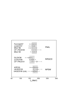
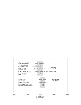
Figure 11: Recent determinations of $f_{B}$ and $f_{D}$ in the quenched approximation.

Recent determinations of $f_{B}$ and $f_{D}$ in the quenched approximation are summarized in Fig. 11 [148] with the references, from top to bottom, [149],[150], [151], [152], [153], [154], [155], [156], [157], [158], and [159] for $f_{B}$, and [149],[150], [151], [152], [153], [157], and [158], and [159] for $f_{D}$. Values of $f_{B}$ derived for a given heavy quark action are consistent. The solid bands, representing the average for a particular heavy quark action, are in agreement with each other. The values of $f_{B}$ and $f_{D}$ in Fig. 11 are also consistent with the LCSR results in [133].

A large source of uncertainty comes from the extrapolation from the scales of the $c$ quark mass to those of the $b$ quark mass. There are other subtle issues, such as the scaling violation from discretization, and the determination of $f_{B}$ at rest and at non-zero momentum [160] and from the temporal $A_{0}$ and spatial $A_{k}$ currents in the matrix element $\langle 0|A_{\mu}|B(P)\rangle=f_{B}P_{\mu}$. More detailed discussion on the above topics can be found [148].

Table 2: $B$ and $D$ meson decay constants with $N_{f}=2$.

Group	$f_{B}$ (MeV)	$\displaystyle{\frac{f_{B}^{N_{f}=2}}{f_{B}^{N_{f}=0}}}$	$f_{D}$ (MeV)	$\displaystyle{\frac{f_{D}^{N_{f}=2}}{f_{D}^{N_{f}=0}}}$
Collins99 [161]	$186(5)(25)(^{+50}_{-0})$	$\simeq 1.26$
MILC’00 [153]	$191(6)(^{+24}_{-18})(^{+11}_{-0})$	$\simeq 1.10$	$215(5)(^{+17}_{-13})(^{+8}_{-0})$	$\simeq 1.08$
MILC’01 ($N_{f}=2+1$) [162]		$1.23(3)(11)$
CP-PACS’00(FNAL) [152]	$208(10)(29)$	1.11(6)	225(14)(40)	1.03(6)
CP-PACS’00(NR) [156]	$204(8)(29)(^{+44}_{-0})$	$1.10(5)$
JLQCD [163]	$190(14)(7)$	$\simeq 1.14$

Calculations of decay constants with dynamical quarks have been available, whose results are listed in Table 2 [148]. It is observed that $f_{B}$ is larger in the unquenched theory. The difference between the quenched and unquenched predictions depends on which type of the valence chiral extrapolation (linear, quadratic or logarithmic [164]) is used. Note that $f_{D}$ may in fact be smaller than the reported value due to discretization effects. It is also observed from Table 2 that the dynamical effect for $D$ mesons is smaller than for $B$ mesons.

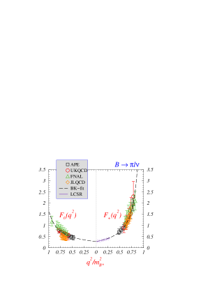
Figure 12: Recent lattice results for $F_{+}(q^{2})$ and $F_{0}(q^{2})$ in the quenched approximation with $F_{+}(0)=F_{0}(0)$. Prediction obtained from LCSR [133] are also shown.

The $B\to\pi$ transition form factors $F_{+}(q^{2})$ and $F_{0}(q^{2})$ have been calculated in lattice QCD recently [165, 166, 167, 168, 169], and the results are presented in Fig. 12 [144]. The data show general agreement among different groups, within the quoted uncertainties. The agreement is especially good for the form factor $F_{+}(q^{2})$. Note that the quenching effects may be significant, particularly for the form factor $F_{0}(q^{2})$ [170]. The lattice results are available only for large $q^{2}$ (smail recoil). Since the bulk of the experimental data is located at small $q^{2}$, one needs to extend the calculation to this region at currently accessible lattice spacings to avoid a model-dependent extrapolation from large $q^{2}$. The new value for the $B\to K^{*}$ form factor at maximal recoil, $T_{1}(0)=T_{2}(0)\equiv T(0)$ defined in Eq. (90), is given by [144]

$$T^{BK^{\ast}}(0)=0.24(5)\left({}^{+1}_{-2}\right)\;,$$ (91)

which is smaller than the LCSR ones [140, 171] shown in Fig. 10.

4.3 Hard-scattering Picture

In the PQCD approach hard dynamics is assumed to dominate in the $B$ meson transition form factors. Soft contribution, though indeed playing a role, is less important because of suppression from the Sudakov mechanism. Unlike QCD sum rules, soft contribution can not be included into the PQCD formalism in a consistent way: if there is no hard gluon exchange to provide a large characteristic scale, twist expansion does not hold. Therefore, soft contribution can not be estimated using the same meson distribution amplitudes resulting from twist expansion. If it has to be added, it must be introduced as an independent input, similar to the treatment in the QCDF approach. The values of these inputs usually come from QCD sum-rule or lattice calculations, which, in principle, can contain perturbative contributions. Then a double counting of the perturbative contribution, which exists already in the one-gluon-exchange diagrams, may not be avoidable.

It has been explained that the internal $\bar{b}$ quark involved in the hard kernel becomes on-shell as the momentum fraction $x$ of the $d$ quark vanishes in Fig. 6 [75]. The contributions to the $B\to\pi$ form factor $F^{B\pi}$ are then logarithmically divergent at twist 2 and linearly divergent at twist 3 in collinear factorization theorem. It has been argued that as the end-point region is important, the corresponding large double logarithms $\alpha_{s}\ln^{2}x$ need to be organized into a jet function $J(x)$ as a consequence of threshold resummation [75]. This jet function, diminishing as $x\to 0,1$, modifies the end-point behavior of meson distribution amplitudes effectively. In [98] the following approximate form has been proposed for convenience,

$$J(x)=\frac{2^{1+2c}\Gamma(3/2+c)}{\sqrt{\pi}\Gamma(1+c)}[x(1-x)]^{c}\;,$$ (92)

where the parameter $c\approx 0.3$ is determined from the best fit to Eq. (38). The above expression is normalized to unity.

Similarly, the inclusion of $k_{T}$ also regulates the end-point singularity, and large double logarithms $\alpha_{s}\ln^{2}k_{T}$ are then produced from higher-order corrections. These double logarithms should be organized to all orders, leading to $k_{T}$ resummation [95, 112]. The resultant Sudakov form factor, constructed in Sec. 3.3 [24], controls the magnitude of $k_{T}^{2}$ to be roughly $O(\Lambda m_{B})$ by suppressing the region with $k_{T}^{2}\sim O(\Lambda^{2})$. The coupling constant $\alpha_{s}(\sqrt{\Lambda m_{B}})/\pi\sim 0.13$ is then small enough to justify the PQCD evaluation of heavy-to-light form factors [25]. Note that either threshold or $k_{T}$ resummation smears the end-point singularity. However, to suppress the soft contribution sufficiently, both resummations are required, such that the reasonable values of the $B\to\pi$ form factors can be obtained.

The $B\to\pi$ form factors $F_{+}$ and $F_{0}$ are written as,

$$F_{+} = \frac{1}{2}(f_{1}+f_{2})\;,$$

$$F_{0} = \frac{1}{2}\left[\left(1+\frac{q^{2}}{m_{B}^{2}}\right)f_{1}+\left(1-\frac{q^{2}}{m_{B}^{2}}\right)f_{2}\right]\;,$$ (93)

with

$$f_{1} = 16\pi m_{B}^{2}C_{F}r_{\pi}\int dx_{1}dx_{2}\int b_{1}db_{1}b_{2}db_{2}\Phi_{+}(x_{1},b_{1})[\phi_{\pi}^{p}(x_{2})-\phi_{\pi}^{t}(x_{2})]E(t^{(1)})h(x_{1},x_{2},b_{1},b_{2})\;,$$ (94)

$$f_{2} = 16\pi m_{B}^{2}C_{F}\int dx_{1}dx_{2}\int b_{1}db_{1}b_{2}db_{2}\Phi_{+}(x_{1},b_{1})$$ (95)

$$\times \Biggl{\{}\left[\phi_{\pi}(x_{2})(1+x_{2}\eta)+2r_{\pi}\left((\frac{1}{\eta}-x_{2})\phi_{\pi}^{t}(x_{2})-x_{2}\phi_{\pi}^{p}(x_{2})\right)\right]E(t^{(1)})h(x_{1},x_{2},b_{1},b_{2})$$

$$+2r_{\pi}\phi_{\pi}^{p}E(t^{(2})h(x_{2},x_{1},b_{2},b_{1})\Biggr{\}}\;.$$

The variable $\eta$ is the pion energy fraction, and the evolution factor given by,

$$E(t)=\alpha_{s}(t)e^{-S_{B}(t)-S_{\pi}(t)}\;.$$ (96)

The explicit expressions of the Sudakov exponents $S_{B}$ and $S_{\pi}$ are referred to [24]. The ratio $r_{\pi}$ is defined as $r_{\pi}=m_{0}/m_{B}$, where the mass scale $m_{0}$, related to the chiral symmetry breaking, comes from the normalization of the two-parton twist-3 distribution amplitudes $\phi_{\pi}^{p,t}$. The contributions from $\phi_{\pi}^{p,t}$ are of leading power [98], and need to be taken into account as mentioned in Sec. 3.2. The first (second) terms in Eq. (95) correspond to Fig. 6(a) [Fig. 6(b)].

The hard function is written as

$$h(x_{1},x_{2},b_{1},b_{2}) = J(x_{2})K_{0}\left(\sqrt{x_{1}x_{2}\eta}m_{B}b_{1}\right)$$ (97)

$$\times\left[\theta(b_{1}-b_{2})K_{0}\left(\sqrt{x_{2}\eta}m_{B}b_{1}\right)I_{0}\left(\sqrt{x_{2}\eta}m_{B}b_{3}\right)\right.$$

$$\left.+\theta(b_{2}-b_{1})K_{0}\left(\sqrt{x_{2}\eta}m_{B}b_{2}\right)I_{0}\left(\sqrt{x_{2}\eta}m_{B}b_{1}\right)\right]\;.$$

The jet function $J(x)$ suppresses the end-point behavior of the pion distribution amplitudes, especially of the twist-3 ones. The hard scales $t$ are defined as

$$t^{(1)} = {\rm max}(\sqrt{x_{2}\eta}m_{B},1/b_{1},1/b_{2})\;,$$

$$t^{(2)} = {\rm max}(\sqrt{x_{1}\eta}m_{B},1/b_{1},1/b_{2})\;.$$ (98)

It is obvious that turning off threshold and $k_{T}$ resummations with $\alpha_{s}$ fixed, Eqs. (94) and (95) are infrared divergent.

As stated in Sec. 4.2, lattice calculations become more difficult in the large recoil region of the light meson. However, this region is the one where PQCD is applicable [24, 172], indicating that the PQCD and lattice approaches complement each other. In LCSR [130, 173] dynamics of the $B\to\pi$ form factors have been assumed to be dominated by a scale larger than $O(\sqrt{\Lambda m_{B}})$. This is the reason the twist expansion into Fock states in powers of $1/m_{B}$ applies to the pion bound state. If this assumption is valid, PQCD should be also applicable to the $B\to\pi$ form factors. I emphasize that the “soft” contributions have different meanings in LCSR and in PQCD. The soft contribution defined in the former has been multiplied by the perturbative Sudakov factor in the latter, such that the soft contribution is large in the former, but small in the latter. A good explanation has been provided in [174]. The definitions of the “hard” contributions are also different, since the twist expansion has been employed for the $B$ meson bound state in PQCD, but not in LCSR. Briefly speaking, the contributions of various orders and powers have been organized in different ways in LCSR and in PQCD (also different in LFQCD discussed below). Hence, the soft dominance concluded in LCSR does not apply to PQCD [175], and there is no conflict between the basic assumptions in the two approaches. For PQCD to be a self-consistent theory, it is only necessary to examine the converegnce of subleading contributions.

For the $B$ meson wave function, the model [25]

$$\Phi_{+}(x,b)=N_{B}x^{2}(1-x)^{2}\exp\left[-\frac{1}{2}\left(\frac{xm_{B}}{\omega_{B}}\right)^{2}-\frac{\omega_{B}^{2}b^{2}}{2}\right]\;,$$ (99)

has been adopted in [98]. The shape parameter $\omega_{B}\sim 0.4$ GeV has been fixed from the fit to the $B\to\pi$ form factors derived from lattice QCD [176] and from LCSR [130]. The normalization constant $N_{B}$ is related to the decay constant $f_{B}=190$ MeV through the relation

$$\int_{0}^{1}dx\phi_{+}(x)=\int_{0}^{1}\Phi(x,b=0)=\frac{f_{B}}{2\sqrt{2N_{c}}}\;.$$ (100)

It is easy to find that Eq. (99) has a maximum at $x\sim\Lambda/m_{B}$. The models for the pion distribution amplitudes can be found in [106].

Figure 13: The $B\to\pi$ form factors $f_{+}$ and $f_{0}$ as functions of $q^{2}$ (GeV²). PQCD results for $\omega_{B}=0.36$, 0.40, and 0.44 GeV are shown in dots. The solid lines correspond to fits to the lattice QCD results [176] with errors. The dashed lines come from LCSR [130].

The relative importance of the twist-2 and twist-3 contributions to $F_{+}(q^{2})$ has been investigated, and the results are listed in Table 3. It is found that the latter are comparable to the former, consistent with the argument that the twist-3 contributions are not power-suppressed. The approximately equal weights of the twist-2 and higher-twist contributions to $F_{+}$ have been also observed in LCSR [126]. We compare the PQCD results of $F_{+}(q^{2})$ and $F_{0}(q^{2})$ for $q^{2}=0\sim 10$ GeV² with those derived from lattice QCD [176] and from LCSR [130] in Fig. 13, where lattice results have been extrapolated to the small $q^{2}$ region. Different extrapolation methods cause uncertainty only of about 5% [177]. The agreement at large recoil indicates that $\omega_{B}\sim 0.4$ GeV is a good choice. The fast rise of the PQCD curves at slow recoil indicates that perturbative calculation becomes unreliable gradually. The range $\omega_{B}=0.40\pm 0.04$ GeV, corresponding to $F_{+}(0)=0.30\pm 0.04$, has been taken as one of the inputs of the PQCD approach to two-body nonleptonic $B$ meson decays.

$q^{2}$ (GeV2)	0.0	1.0	2.0	3.0	4.0	5.0	6.0	7.0	8.0	9.0	10.0
twist 2	0.120	0.128	0.138	0.148	0.159	0.172	0.188	0.204	0.223	0.243	0.270
twist 3	0.177	0.193	0.210	0.230	0.253	0.279	0.308	0.344	0.385	0.432	0.487
total	0.297	0.321	0.348	0.378	0.412	0.451	0.496	0.548	0.608	0.675	0.757

Table 3: Contributions to $f_{+}(q^{2})$ from the twist-2 and two-parton twist-3 pion distribution amplitudes.

The same range of $\omega_{B}$ has been adopted in the evaluation of the $B\to\rho$ transition form factors. The results, displayed in Fig. 14, are also consistent with those from LCSR [178] at small $q^{2}$. It is found that the symmetry relation in Eq. (109) below holds very well: $A_{1}$ is larger than $V$ only by 2% in the large recoil region, even after considering the pre-asymptotic forms of the $\rho$ meson distribution amplitudes [106]. Taking the fast recoil limit with $\eta\to 1$ and assuming the asymptotic behavior $\phi_{\rho}^{v}=\phi_{\rho}^{a}$, the above form factors are found to obey the symmetry relations [72, 179],

$$V=A_{1}\;,\;\;\;A_{2}=A_{1}-2r_{\rho}A_{0}\;.$$ (101)

Note that the form factors, treated as nonperturbative objects, are not calculated in [72]. Instead, the diagrams in Fig. 6 under an infrared regularization scheme are regarded as perturbative corrections to the relations in Eq. (101). For the application of the PQCD approach to the radiative decay $B\to K^{*}\gamma$, refer to [180].

Figure 14: The $B\to\rho$ form factors $V$, $A_{0}$, $A_{1}$ and $A_{2}$ as functions of $q^{2}$. PQCD results are given in dots. The solid lines come from light-cone sum rules.

4.4 Power Corrections

SCET provides a systematic framework for discussing power corrections to heavy-to-light transitions at large recoil. Here I review the heavy quark expansion of the $B$ meson transition form factors in SCET. It will be observed that SCET is a powerful tool of deriving the relations among various form factors in the large energy limit. There are three independent form factors associated with decays into pseudoscalars, and seven independent form factors with decays into vector mesons. In the former case except for the form factors $F_{+,0}$ introduced in Eq. (82), another one $F_{T}$ is defined via the matrix element,

$$\langle P(P_{2})|\bar{q}\,\sigma^{\mu\nu}q_{\nu}b|\bar{B}(P_{1})\rangle=\frac{iF_{T}(q^{2})}{m_{B}+m_{P}}\left[q^{2}(P_{1}^{\mu}+P_{2}^{\mu})-(m_{B}^{2}-m_{P}^{2})\,q^{\mu}\right]\;.$$ (102)

At leading power, the number of independent form factors reduces. Assume the energy $E\sim O(m_{B})$ of the final state meson, which is related to the momentum transfer $q^{2}$ by $E=(m_{B}^{2}+m_{P}^{2}-q^{2})/(2m_{B})$. The universal functions $A_{P}^{(0)}(E,v,\bar{n})$ and $A_{V}^{(0)}(E,v,\bar{n},\epsilon)$, defined via the matrix elements, $\langle P(P_{2})|\xi\,\Gamma\,W\,h_{v}|\bar{B}(P_{1})\rangle$ and $\langle V(P_{2},\epsilon)|\bar{\xi}\,\Gamma\,W\,h_{v}|\bar{B}(P_{1})\rangle$, respectively, can be decomposed into their most general independent Dirac structures allowed by Lorentz invariance and parity [72, 179],

$$A_{P}^{(0)}(E,v,\bar{n}) = 2E\,\xi_{P}^{(0)}(E)\;,$$

$$A_{V}^{(0)}(E,v,\bar{n},\epsilon) = -2E\,\not\epsilon_{T}^{\ast}\,\gamma_{5}\,\xi_{T}^{(0)}(E)-2E\,(v\cdot\epsilon^{\ast})\,\gamma_{5}\,\xi_{\parallel}^{(0)}(E)\;.$$ (103)

That is, only one universal form factor $\xi_{P}^{(0)}(E)$ is left for the former, and two form factors, $\xi_{T}^{(0)}(E)$ and $\xi_{\parallel}^{(0)}(E)$, corresponding to transversely and longitudinally polarized light vector mesons, respectively, for the latter.

It has been argued [59] that the small expansion parameter in SCET should be taken as $\lambda\sim\sqrt{\Lambda/E}$ for the heavy-to-light transition form factors. The pion emitted in a heavy-to-light decay at large recoil carries momentum scaling like $p_{\pi}\sim(\Lambda^{2}/E,E,\Lambda)$. This pion is produced in a highly asymmetric state, composing of a soft quark with momentum $p_{s}\sim(\Lambda,\Lambda,\Lambda)$ and a collinear jet. This jet must have an invariant mass squared $p_{c}^{2}=(p_{\pi}-p_{s})^{2}\sim E\Lambda=\lambda^{2}E^{2}$. Hence, one has the expansion parameter $\lambda\sim\sqrt{\Lambda/E}$ based on the above kinematical consideration. In this case soft fields carrying momenta of order $\Lambda$ scale like $E(\lambda^{2},\lambda^{2},\lambda^{2})$ and are assigned as being usoft as stated in Sec. 3.2.

One decomposes the matrix element of the heavy-to-light current in full QCD as

$$\langle P(P_{2})|\bar{q}\,\Gamma\,Q|\bar{B}(P_{1})\rangle = {\rm tr}\left[A_{P}^{(++)}\,\frac{\not n\not{\bar{n}}}{4}\,\Gamma\,\frac{1+\not v}{2}\right]+{\rm tr}\left[A_{P}^{(+-)}\,\frac{\not n\not{\bar{n}}}{4}\,\Gamma\,\frac{1-\not v}{2}\right]$$ (104)

$$+\,{\rm tr}\left[A_{P}^{(-+)}\,\frac{\not{\bar{n}}\not n}{4}\,\Gamma\,\frac{1+\not v}{2}\right]+{\rm tr}\left[A_{P}^{(--)}\,\frac{\not{\bar{n}}\not n}{4}\,\Gamma\,\frac{1-\not v}{2}\right]\;,$$

using the projectors $(1\pm\not v)/2$, $\not n\not{\bar{n}}/4$ and $\not{\bar{n}}\not n/4$ on the large and small components of the quark fields, labelled by $+$ and $-$, respectively. The definition for decays into vector mesons is analogous. The functions $A_{P}^{(kl)}$ and $A_{V}^{(kl)}$ with $k,l=+,-$ can again be decomposed as

$$A_{P}^{(kl)}(E,v,\bar{n}) = 2E\,f_{P}^{(kl)}(E)\;,$$

$$A_{V}^{(kl)}(E,v,\bar{n},\epsilon) = -2E\,\not\epsilon_{T}^{\ast}\,\gamma_{5}\,f_{T}^{(kl)}(E)-2E\,(v\cdot\epsilon^{\ast})\,\gamma_{5}\,f_{\parallel}^{(kl)}(E)\;.$$ (105)

Among the $4+8$ form factors $f_{P}^{(kl)}$ and $f_{T,\,\parallel}^{(kl)}$ only $3+7$ are independent due to the equations of motion for light and heavy quarks in QCD and translational invariance,

$$q^{\mu}\langle P|\bar{q}\,\gamma_{\mu}\,b|B\rangle = (m_{b}-m_{q})\,\langle P|\bar{q}\,b|B\rangle\;,$$

$$q^{\mu}\langle V|\bar{q}\,\gamma_{\mu}\gamma_{5}\,b|B\rangle = -(m_{b}+m_{q})\,\langle V|\bar{q}\,\gamma_{5}\,b|B\rangle\;,$$ (106)

with $q=P_{1}-P_{2}$.

With the SCET expansion of the heavy-to-light currents, it is easy to identity the scaling of the above form factors:

$$f_{i}^{(++)}(E)=\xi_{i}^{(0)}(E)\,\Big{(}1+O(\alpha_{s},\lambda)\Big{)}\;,$$

$$f_{i}^{(+-)}(E)\sim\lambda\,f_{i}^{(++)}(E)\;,\qquad f_{i}^{(-+)}(E)\sim\lambda\,f_{i}^{(++)}(E)\;,\qquad f_{i}^{(--)}(E)\sim\lambda^{2}f_{i}^{(++)}(E)\;.$$ (107)

At $O(\lambda)$, the neglect of $f_{i}^{(--)}(E)$ leaves 3+6 form factors for pseudoscalar and vector mesons, respectively. The equations of motion in Eq. (106) give two more constraints at this order. Therefore, one has 2+5 independent form factors, implying 1+2 form factor relations.

At $O(\lambda)$, the three form factor relations are written as [59]

$$R_{P} = \frac{F_{+}-F_{0}}{F_{T}}=\frac{q^{2}}{m_{B}\,(m_{B}+m_{P})}\left(1+O(\alpha_{s},\lambda^{2})\right)\;,$$

$$R_{T} = \frac{\displaystyle\left(1-\frac{q^{2}}{m_{B}^{2}}\right)T_{1}-T_{2}+\frac{q^{2}}{m_{B}^{2}}\left(1+\frac{m_{V}}{m_{B}}\right)A_{1}}{\displaystyle\left(1-\frac{q^{2}}{m_{B}^{2}}\right)V}=\frac{q^{2}}{m_{B}\,(m_{B}+m_{V})}\left(1+O(\alpha_{s},\lambda^{2})\right)\;,$$

$$R_{\parallel} = \frac{\displaystyle\left(1+\frac{m_{V}}{m_{B}}\right)A_{1}-\left(1-\frac{m_{V}}{m_{B}}\right)\left(1-\frac{q^{2}}{m_{B}^{2}}\right)A_{2}-2\,\frac{m_{V}}{m_{B}}\left(1-\frac{q^{2}}{m_{B}^{2}}\right)A_{0}}{\displaystyle T_{2}-\left(1-\frac{q^{2}}{m_{B}^{2}}\right)T_{3}}\;,$$ (108)

$$= \frac{q^{2}}{m_{B}^{2}}\left(1+O(\alpha_{s},\lambda^{2})\right)\;,$$

for the decays into light pseudoscalar, transversely and longitudinally polarized mesons, respectively. As $q^{2}\to 0$, the left-hand sides of the above relations vanish exactly. Other form factor relations, which receive $O(\lambda)$ corrections, have been also derived in [59]:

$$\left(1-\frac{q^{2}}{m_{B}^{2}}\right)V-\left(1+\frac{m_{V}}{m_{B}}\right)^{2}A_{1}=O(\lambda)\;,\qquad\left(1-\frac{q^{2}}{m_{B}^{2}}\right)T_{1}-T_{2}=\frac{q^{2}}{m_{B}^{2}}\,O(\lambda)\;.$$ (109)

The above result differs from that in [57], where the first equation in (109) does not receive an $O(\lambda)$ correction.

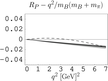
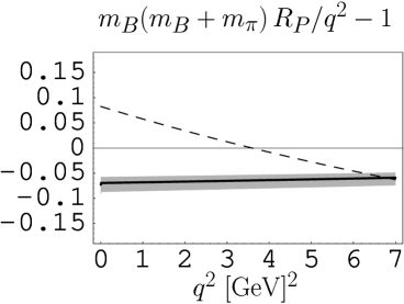
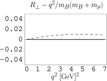
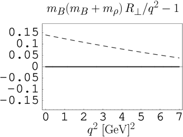
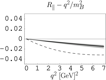
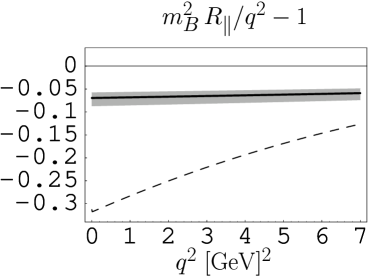
Figure 15: Test of the relations in Eq. (108) for $B\to\pi$ and $B\to\rho$ form factors. The dashed line corresponds to the form factors predicted from LCSR [130, 140]. The solid line is the $O(\lambda^{0})$ result including the $\alpha_{s}$ corrections [72].

To test the form factor relations in Eq. (108), one substitutes the form factors derived from LCSR [130, 140] into the left-hand sides and compare the outcomes with the right-hand sides. The $O(\alpha_{s})$ corrections to the heavy quark limit have been included on the right-hand sides. The results are displayed in Fig. 15 [59]. The ratios $R_{P,T,\parallel}$ minus the corresponding values in the symmetry limit are shown on the left-hand side. The tensor form factors are evaluated at the scale $m_{b}$. The grey error band reflects the theoretical uncertainty from varying the scale of $\alpha_{s}$ from $m_{b}/2$ to $2m_{b}$. The difference between the dashed and solid curves is an estimate of $O(\lambda^{2})$ or $O(\alpha_{s}\lambda)$ corrections, which are at most 3% deviations from zero for $q^{2}$ up to 7 GeV². $R_{P,T,\parallel}$ divided by their symmetry limits minus 1 are shown on the right-hand side of Fig. 15. It is expected that deviations from 0 are of $O(\lambda^{2})$ and/or $O(\alpha_{s})$, since the $q^{2}$ suppression has been divided out.

Note that the scaling behavior of the quark fields and of the meson states with $\lambda$ is not sufficient to determine the scaling behavior of form factors. Considering soft contribution to the form factor, the $u$ quark created in the decay of the $b$ quark carries almost all the energy of the light meson, while the spectator quark is soft. To leading order in $\Lambda/E$, the interaction of energetic quarks with soft gluons is described by the eikonal Lagrangian [179, 181]

$${\cal L}_{\rm eik}=\bar{q}_{n}\,\frac{\not n}{2}\,(i\,\bar{n}\cdot D)\,q_{n}+O(1/E_{q}),$$ (110)

where $q_{n}(x)=e^{iE_{q}\bar{n}\cdot x}\not{\bar{n}}\not{n}q(x)/4$ are the large components of the light quark spinor field. Even for light-cone dominated processes this is an atypical configuration (the preferred one having nearly equal momenta of the quark and antiquark). For this reason, although the interaction in Eq. (110) is spin-symmetric, the symmetry is not realized in the hadronic spectrum, and there exists no relation among the soft contributions to the form factors of pseudoscalar and vector mesons. Furthermore, the probability that such an asymmetric parton configuration hadronises into a light meson depends on the energy of the meson. Hence, the soft contributions to the form factors are energy-dependent functions, whose absolute normalization is not known.

In this respect SCET applied to heavy-to-light decays at large recoil differs from HQET for $B\to D^{(*)}$ form factors. In the case of heavy-heavy form factors, spin symmetry relates pseudoscalar and vector mesons, and the Isgur-Wise form factor $\xi(v\cdot v^{\prime})$ is independent of the heavy quark mass. One obtains non-trivial form factor relations beyond the leading order in $\lambda$, because the heavy quark flavor symmetry also relates the initial and final hadronic states.

Recently, an expansion parameter $\lambda\sim\Lambda/E$ for heavy-to-light form factors has been proposed [182], which differs from $\lambda\sim\sqrt{\Lambda/E}$ discussed above [57, 59]. For $\lambda\sim\sqrt{\Lambda/E}$, the external pion, whose momentum scales like $p_{\pi}\sim E(1,\lambda^{4},\lambda^{2})$, cannot be built up from the combination of a generic usoft momentum $p_{s}\sim E(\lambda^{2},\lambda^{2},\lambda^{2})$ with a generic collinear momentum $p_{c}\sim E(1,\lambda^{2},\lambda)$. It implies that the soft mechanism is strongly suppressed in this picture. For $\lambda\sim\Lambda/E$, the pion momentum scales like a collinear momentum. In order to make a light meson out of collinear particles and soft particles, one has to require the minus component of the total soft momentum, which would scale like $E\lambda$, to be accidentally small, of order $E\lambda^{2}$. However, this implies a phase-space suppression of $O(\Lambda/E)$ as explained in [98]. It has been expected [182] that under the different choices of the expansion parameters, the violations of heavy quark symmetry relations between form factors may start at different power of $\Lambda/E$. From the view point of the PQCD approach, the spectator on the pion side is as energetic as the collinear particles. That is, all the momenta scale like a collinear momentum, and there is no phase-space suppression.

4.5 Radiative Corrections

Form factors for heavy-to-light transitions are presumably dominated by nonperturbative QCD dynamics at small momentum transfer and not computable in perturbation theory. Charles et al. have shown that certain symmetries apply to this soft contribution, when the momentum of the final light meson is large [179]. These symmetries reduce the number of independent form factors from ten to three as shown in Sec. 4.4. The corresponding symmetry relations for the form factors are broken by power corrections discussed above and by radiative corrections. In this subsection I review the evaluation of the symmetry-breaking corrections at first order in the strong coupling constant $\alpha_{s}$, which are dominated by short-distance contributions. The formalism adopted below is referred to as the QCDF approach [72].

In the absence of a hard spectator interaction shown in Fig. 16(a), the light meson is produced in a parton configuration, in which the $u$ quark carries all the momentum of the meson, up to an amount of $O(\Lambda)$ in the $B$ meson rest frame. The hard part of the vertex correction in Fig. 16(b) does not respect the symmetry relations, but can be accounted for in perturbation theory by multiplicatively renormalizing the current $[u_{n}\Gamma b_{v}]_{\rm eff}$ in the effective theory. A hard interaction with the spectator quark shown in Figs. 16(c) and 16(d) allows the meson to be formed in a preferred configuration, in which the momentum is distributed nearly equally between the two quarks.

The soft contribution scales like [18]

$$F_{+,0,T}^{\rm soft}(q^{2}\approx 0)\sim\xi_{P}(E\approx m_{B}/2)\sim\sqrt{\frac{m_{B}}{E}}\left(\frac{\Lambda}{E}\right)^{\!3/2}\sim\left(\frac{\Lambda}{M}\right)^{\!3/2}\;.$$ (111)

For the hard contribution, both quarks that form the light meson have momenta of $O(m_{B})$, and the gluon in Figs. 16(c) and 16(d) has virtuality of order $\Lambda m_{B}$. The resulting scaling behaviour for the pseudoscalar meson form factors is

$$F_{+,0,T}^{\rm hard}(q^{2}\approx 0)\sim\alpha_{s}(\sqrt{\Lambda m_{B}})\,\left(\frac{\Lambda}{m_{B}}\right)^{\!3/2}\;.$$ (112)

Therefore, the hard spectator interaction is suppressed by one power of $\alpha_{s}$ relative to the soft contribution.

Figure 16: Different contributions to the $B\to P(V)$ transition. (a) Soft contribution (soft interactions with the spectator antiquark $\bar{q}^{\prime}$ are not drawn). (b) Hard vertex renormalization. (c,d) Hard spectator interaction.

The QCDF formula for a heavy-light form factor at large recoil at leading power in $1/m_{B}$ is then written as [72]

$$F_{i}(q^{2})=C_{i}\,\xi_{P}(E)+\phi_{B}\otimes T_{i}\otimes\phi_{P}\;.$$ (113)

The soft form factor $\xi_{P}(E)$, defined in Eq. (103) and represented by Fig. 16(a), obeys the symmetries discussed above. The hard-scattering kernel $T_{i}$ from Figs. 16(c) and 16(d) is convoluted with the light-cone distribution amplitudes of the $B$ meson and of the light pseudoscalar meson, for which the endpoint divergence together with some finite contribution have been absorbed into the leading soft term. The coefficient $C_{i}=1+O(\alpha_{s})$ is the hard vertex renormalization from Fig. 16(b). The correction at $O(\alpha_{s})$ from the hard vertex renormalization and from the hard spectator interaction have been obtained in [28, 72].

To absorb the end-point singularities, the factorization scheme has been defined by imposing the condition,

$$F_{+}\equiv\xi_{P},\qquad\ V\equiv\frac{m_{B}+m_{V}}{m_{B}}\,\xi_{\perp},\qquad A_{0}\equiv\frac{E}{m_{V}}\,\xi_{\parallel},$$ (114)

exactly to all orders in perturbation theory, similar to the DIS scheme for inclusive processes. Having fixed the factorization scheme, all other form factors can be expressed, for example, as

$$F_{0} = \frac{2E}{m_{B}}\,\xi_{P}\,\left[1+\frac{\alpha_{s}\,C_{F}}{4\pi}\,\left(2-2\,L\right)\right]+\frac{\alpha_{s}\,C_{F}}{4\pi}\,\Delta F_{0}\;,$$ (115)

$$F_{T} = \frac{M+m_{P}}{M}\,\xi_{P}\,\left[1+\frac{\alpha_{s}\,C_{F}}{4\pi}\,\left(\ln\frac{m_{b}^{2}}{\mu^{2}}+2\,L\right)\right]+\frac{\alpha_{s}\,C_{F}}{4\pi}\,\Delta F_{T}\;,$$ (116)

with the notation,

$$L=-\frac{2E}{m_{B}-2E}\,\ln\frac{2E}{m_{B}}\;.$$ (117)

Note $L\to 1$ for $E\to m_{B}/2$ ($q^{2}\to 0$).

The $O(\alpha_{s})$ corrections to the form factors are given by

$$\Delta F_{0}=\frac{m_{B}-2E}{2E}\,\Delta F_{P}\;,\qquad\Delta F_{T}=-\frac{m_{B}+m_{P}}{2E}\,\Delta F_{P}\;,$$ (118)

with the quantity,

$$\Delta F_{P}=\frac{8\pi^{2}f_{B}f_{P}}{N_{C}m_{B}}\int dk^{+}\frac{\phi_{+}(k^{+})}{k^{+}}\int du\frac{\phi(u)}{\bar{u}}\;.$$ (119)

The theoretical uncertainties in the computation of the hard-scattering correction from the moments of the meson distribution amplitudes [183] and from the $B$ meson decay constant are all contained $\Delta F_{P}$.

Equation (113) has been further elucidated in the framework of SCET [63]. At leading power in $1/m_{b}$ and all orders in $\alpha_{s}$, a $B\to P$ transition form factor $F$ can be split into factorizable and nonfactorizable components,

$$F(E) = f^{\rm F}(E)+f^{\rm NF}(E)\;,$$

$$f^{\rm F}(E) = \frac{f_{B}f_{P}}{E^{2}}\int_{0}^{1}\!\!\!\!dz\!\int_{0}^{1}\!\!\!\!dx\!\int_{0}^{\infty}\!\!\!\!\!dk^{+}\,T(z,E,\mu_{\rm 0})$$ (120)

$$\quad\times J(z,x,k^{+},E,\mu_{\rm 0},\mu)\phi_{P}(x,\mu)\phi_{+}(k^{+},\mu)\,,$$

$$f^{\rm NF}(E) = C_{i}(E,\mu)\>\xi_{i}(E,\mu)\,.$$ (121)

Compared to Eq. (113), the hard-scattering kernel has been further factorized into a function $T$ characterized by the scale $m_{b}$ and a jet function $J$ characterized by the scale $\mu_{\rm 0}\simeq\sqrt{m_{b}\Lambda}$. Hence, the hard coefficients $C_{k}$ and $T$ are calculated in an expansion in $\alpha_{s}(m_{b})$. The jet function $J$ is calculable in terms of a matrix element involving $\alpha_{s}(\sqrt{\Lambda m_{b}})$. That is, the contributions characterized by $m_{b}$ and $\sqrt{m_{b}\Lambda}$ have been clearly separated. Endpoint singularities arise only in the soft, nonperturbative form factors $\xi_{i}(E,\mu)$. The convolution integrals in the factorizable terms are infrared finite in collinear factorization theorem.

I explain the difference between the QCDF formulas based on collinear factorization and those in the PQCD approach based on $k_{T}$ factorization. In the former the piece with an end-point singularity in collinear factorization theorem has been regularized and absorbed into the soft term $f^{\rm NF}$. In $k_{T}$ factorization theorem the end-point singularity is absent, and both $f^{\rm NF}$ and $f^{\rm F}$ can be formulated into the factorization formulas. Since $f^{\rm NF}$ remains in the formulas, the form factor symmetry relations at large recoil are still respected in the PQCD approach, which are then modified by the less important term $f^{\rm F}$. This has been shown explicitly in Eq. (101), contrary to the criticism in [72]. It is then realized that the definition of soft contributions is in fact ambiguous, depending on the theoretical framework that is adopted. In QCDF the soft contribution refers to the one with the end-point singularity in collinear factorization theorem (plus an arbitrary infrared-finite piece related to a factorization scheme). In PQCD it refers to the one from a large (but arbitrary) coupling constant. Therefore, the hard-scattering terms in both approaches [in Eq. (113) and in Eq. (95)] also collect different contributions.

To be more specific, I compare the explicit expression for the form factor $F_{+}$ derived based on Eq. (121) [63],

$$F_{+}(E) = N_{0}\int dxdk^{+}\left[\frac{2E-m_{B}}{m_{B}}C_{a}(E,\mu_{\rm 0})+\frac{2E}{m_{b}}C_{b}(E,\mu_{\rm 0})\right]$$ (122)

$$\times\frac{\alpha_{s}(\mu_{\rm 0})}{x\,k^{+}}\phi_{\pi}(x)\phi_{+}(k^{+})+C(E,\mu)\,\zeta(E,\mu)\,,$$

with the constant,

$$N_{0}=\frac{\pi C_{F}}{4}\frac{f_{B}f_{\pi}m_{B}}{N_{c}E^{2}}\;,$$ (123)

to Eq. (93). The Wilson coefficients satisfy $C_{a}=C_{b}=1$ at the tree level. Removing all the Sudakov factors and dropping the twist-3 contributions, $F_{+}$ in Eq. (93) from the PQCD approach reduces to

$$F_{+}(E) = N_{0}\alpha_{s}m_{B}\int dx_{1}dx_{2}\left(\frac{\eta}{x_{1}x_{2}}+\frac{\eta+1}{x_{1}x_{2}}+\frac{1}{x_{1}x_{2}^{2}}\right)\phi_{\pi}(x_{2})\phi_{+}(x_{1})\;.$$ (124)

Using the variable change $\eta=2E/m_{B}-1$, it is easy to identify the three terms in Eq. (124) as the three terms in Eq. (122) in sequence. The third term in Eq. (124) with the end-point singularity comes from the term 1 in the coefficient $1+x_{2}\eta$ of $\phi_{\pi}$ in Eq. (95). This piece obeys the large-energy symmetry mentioned above. The term $x_{2}\eta$, whose $x_{2}$ cancels a power of $x_{2}$ in the denominator, corresponds to the hard-scattering piece in Eq. (122).

A study of the relative importance of soft and hard dynamics has been done in the framework of QCD sum rules [174]. The soft contribution without Sudakov suppression was estimated to be 0.22 (corresponding to $f_{B}\sim 130$ MeV). The soft contribution to $f_{B}F^{B\pi}$ obtained in [126] is consistent with the above value. It was then shown that the Sudakov effect decreases the soft contribution by a factor 0.4-0.7, depending on infrared cutoffs for loop corrections to the weak decay vertex. Therefore, the soft contribution turns out to be about 0.09-0.15, and smaller than the perturbative contribution about 0.19. It is then possible that the $B\to\pi$ form factors receive significant perturbative contributions, in spite of the large theoretical uncertainty in sum rules, for example, from the variation of the Borel mass [126].

The QCDF formalism has been applied to the study of the forward-backward asymmetry in the rare decay $B\to V\ell^{+}\ell^{-}$, where $V$ is a vector meson [184]. Below I discuss the simpler modes $B\to V\gamma$ [185, 186]. The hadronic matrix elements are written as,

$$\langle V\gamma(\epsilon)|O_{i}|B\rangle=\Big{[}F^{BV}T^{I}_{i}+\!\int^{1}_{0}\!\!d\xi\,dv\,T^{II}_{i}(\xi,v)\phi_{B}(\xi)\phi_{V}(v)\Big{]}\!\cdot\epsilon\;,$$ (125)

where $\epsilon$ is the photon polarization vector and the operators $O_{i}$ come from the effective weak Hamiltonian. The soft form factor $F^{BV}$ for the $B\to V$ transition obeys the symmetry relations in the large energy limit. In QCDF the next-to-leading-order hard corrections to the weak decay vertex in Fig. 17 contribute to $T_{i}^{I}$ [187]. These contributions are dominated by scales of $O(m_{b})$ and infrared finite. $T^{II}_{i}$ involves the hard scattering of the spectator shown in Fig. 18.

Figure 17: Typical $O(\alpha_{s})$ contribution to the hard-scattering kernel $T^{I}_{i}$. The crosses represent the photon vertices.

Figure 18: Typical $O(\alpha_{s})$ contribution to the hard-scattering kernel $T^{II}_{i}$.

For the $B\to V\gamma$ decay, both the type I and type II contributions can be expressed in terms of the matrix element $\langle O_{7}\rangle$:

$$A(B\to V\gamma)=\frac{G_{F}}{\sqrt{2}}\left[\lambda_{u}^{(s)}a^{u}_{7}+\lambda_{c}^{(s)}a^{c}_{7}\right]\langle V\gamma|O_{7}|B\rangle\;,$$ (126)

where $\lambda_{u,c}^{(s)}$ are the products of the CKM matrix elements, the coefficients $a_{7}^{(u,c)}$ consist of the Wilson coefficient $C_{7}$ and the contributions from the type-I and type-II hard-scattering corrections. It has been observed that the leading-order value is enhanced by the $T^{I}$-type correction. The net enhancement of $a_{7}$ at the next-to-leading order increases the branching ratios as illustrated in Fig. 19 [188]. The residual scale dependence for $B(\bar{B}\to\bar{K}^{*0}\gamma)$ and $B(B^{-}\to\rho^{-}\gamma)$ at leading and next-to-leading orders is also exhibited.

Figure 19: Dependence of the branching ratios $B(\bar{B}^{0}\to\bar{K}^{*0}\gamma)$ and $B(B^{-}\to\rho^{-}\gamma)$ on the renormalization scale $\mu$, where the leading-order contributions (dotted lines), the next-to-leading-order contributions including only type-I corrections (dash-dotted lines), and the complete next-to-leading-order contributions (solid lines) are explicitly shown.

The branching ratios of the exclusive radiative decays have been measured to be $B(B^{0}\!\to K^{*0}\gamma)=(4.44\pm 0.35)\times 10^{-5}$ and $B(B^{+}\!\to K^{*+}\gamma)=(3.82\pm 0.47)\times 10^{-5}$ [189]. For the $B\to\rho\gamma$ decay, only upper bound exists. The leading-order results from QCDF have more or less saturated the experimental data, and the inclusion of the next-to-leading-order contributions overshoot the data. Note that the transition form factor $F^{BV}$ and the distribution amplitudes $\phi_{B}$ and $\phi_{V}$ are both the independent inputs in QCDF. The large predicted branching ratio about $B(B^{0}\!\to K^{*0}\gamma)=7\times 10^{-5}$ could indicate a double counting of hard contributions between the two terms in Eq. (125). Therefore, the basic assumption of QCDF, in which the transition form factor is a completely soft object, requires a more careful examination.

4.6 Light-Front QCD

In the non-relativistic quark model, wave functions best resemble meson states in the rest frame, or where the meson velocities are small. Therefore, the form factors calculated in this model are reliable only at small recoil. At large recoil, relativistic effects must be taken into account. A consistent and fully relativistic treatment [190] of quark spins and the center-of-mass motion can be carried out in LFQCD [191, 192, 193]. This method has several advantages: the light-front (LF) wave function is manifestly Lorentz invariant in terms of the momentum fraction variables (in “+” components), which is in analogy with parton distributions in the infinite momentum frame. Hadron spin can be correctly constructed using the Melosh rotation. The kinematic subgroup of the LF formalism has the maximal number of interaction-free generators, including the boost operator which describes the center-of-mass motion of the bound state.

LFQCD has been applied to the heavy-to-heavy and heavy-to-light transition form factors [194, 195, 196, 197]. However, the form factors were calculated only for $q^{2}\leq 0$, whereas physical decays occur in the time-like region with $0\leq q^{2}\leq(m_{i}-m_{f})^{2}$, $m_{i,f}$ being the initial and final meson masses. Hence, extra assumptions are needed to extrapolate the form factors from the space-like region to the time-like region [198, 199]. Recently, the $P\to P$ transition form factors were calculated in the entire range of $q^{2}$ [200, 201], such that the additional extrapolation is no longer required. This is based on the observation [202] that in the frame where the momentum transfer is purely longitudinal, i.e., $q_{T}=0$, the invariant $q^{2}=q^{+}q^{-}$ covers the entire range of momentum transfer. The price to pay is that, besides the conventional valence-quark contribution, one must also consider the nonvalence configuration (or the so-called Z graph) in order to maintain covariance. The nonvalence contribution vanishes at $q^{+}=0$, but is expected to be more important for heavy-to-light transitions near zero recoil [194, 198, 202, 203]. Prescriptions for treating this nonvalence configuration have been proposed. For example, the authors of [201] considered the effective higher Fock state, and calculated the contribution in chiral perturbation theory. For a relevant discussion of covariance in the LFQCD framework, refer to [204].

Figure 20: (a) The Feynman triangle diagram. (b) corresponds to the LF nonvalence configuration and diagram (c) to the valence one. Filled and empty circles indicate vertex functions and LF wave functions, respectively.

Below I mention the other two prescriptions [205, 206]. Start with the matrix element,

$$\langle P^{\prime}(P_{2})|\bar{Q^{\prime}}\gamma^{\mu}Q|P(P_{1})\rangle=F_{+}(q^{2})(P_{1}+P_{2})^{\mu}+F_{-}(q^{2})~{}q^{\mu}\;,$$ (127)

where $q=P_{1}-P_{2}$ is the momentum transfer. The form factor $F_{0}$ is related to $F_{\pm}(q^{2})$ by

$$F_{0}(q^{2})=F_{+}(q^{2})+{q^{2}\over{m_{P}^{2}-m_{P^{\prime}}^{2}}}F_{-}(q^{2})\;.$$ (128)

Assume a vertex function $\Lambda_{P}$ [194, 195], related to bound state $Q\bar{q}$ of the meson $P$. The quark-meson diagram in Fig. 20(a) gives

$$\langle P^{\prime}(P_{2})|\bar{Q^{\prime}}\gamma^{\mu}Q|P(P_{1})\rangle=-\int{d^{4}p_{1}\over{(2\pi)^{4}}}\Lambda_{P}\Lambda_{P^{\prime}}tr\Bigg{[}\gamma_{5}{i(\not{\!p_{3}}+m_{3})\over{p_{3}^{2}-m^{2}_{3}+i\epsilon}}\gamma_{5}{i(\not{\!p_{2}}+m_{2})\over{p_{2}^{2}-m^{2}_{2}+i\epsilon}}\gamma^{\mu}{i(\not{\!p_{1}}+m_{1})\over{p_{1}^{2}-m^{2}_{1}+i\epsilon}}\Bigg{]}\;,$$ (129)

with $p_{2}=p_{1}-q$ and $p_{3}=p_{1}-P_{1}$. Consider the poles in denominators and perform the integration over the “energy” $p_{1}^{-}$ in Eq. (129). One derives

$$\langle P^{\prime}(P_{2})|\bar{Q^{\prime}}\gamma^{\mu}Q|P(P_{1})\rangle = \int^{q}_{0}[d^{3}p_{1}]\Bigg{(}{\Lambda_{P}\over{S_{1}+S_{3}}}I^{\mu}{\Lambda_{P^{\prime}}\over{S_{2}+S_{3}}}\Bigg{)}\Bigg{|}_{S_{1}=0}\;,$$ (130)

$$+ \int^{P}_{q}[d^{3}p_{1}]\Bigg{(}{\Lambda_{P}\over{S_{1}+S_{3}}}I^{\mu}{\Lambda_{P^{\prime}}\over{S_{2}+S_{3}}}\Bigg{)}\Bigg{|}_{S_{3}=0}\;,$$

with the definitions,

$$[d^{3}p_{1}]=dp^{+}_{1}d^{2}p_{1T}/(64\pi^{3}\prod_{i=1}^{3}p^{+}_{i})\;,$$

$$I^{\mu}=tr[\gamma_{5}(\not{\!p_{3}}+m_{3})\gamma_{5}(\not{\!p_{2}}+m_{2})\gamma^{\mu}(\not{\!p_{1}}+m_{1})]\;,$$

$$S_{i}\equiv p^{-}_{i}-p^{-}_{i{\rm on}}\;,\;\;\;\;i=1,2,3\;,$$

$$p^{-}_{1(3)}=P^{-}_{1\rm on}-p^{-}_{3(1){\rm on}}\;,$$

$$p^{-}_{i{\rm on}}=(m_{i}^{2}+p^{2}_{iT})/(2p_{i}^{+})\;.$$ (131)

$p^{-}_{2}$ is equal to $p^{-}_{3{\rm on}}-P^{-}_{2\rm on}$ ($P^{-}_{2\rm on}-p^{-}_{3{\rm on}}$) in the first (second) term of Eq. (130). The non-pointlike vertex structures $\Lambda_{P}$ are necessary in order to smear the divergences in the integrals.

Associate

$$R^{\rm v}_{1,2} = {\sqrt{P_{1}^{+}p^{+}_{1}p^{+}_{2}}\over{2\sqrt{p_{1{\rm on}}\cdot p_{2{\rm on}}+m_{1}m_{2}}}}\;,$$

$$R^{\rm n}_{2,3} = {\sqrt{P_{2}^{+}p^{+}_{2}p^{+}_{3}}\over{2\sqrt{p_{2{\rm on}}\cdot p_{3{\rm on}}-m_{2}m_{3}}}}\;,$$ (132)

with the valence and nonvalence configurations of the Melosh transformation [207] $R^{S,S_{z}}_{\lambda_{1},\lambda_{2}}$, which creats a state of definite spin ($S,S_{z}$) out of LF helicity ($\lambda_{1},\lambda_{2}$) eigenstates [201, 208, 209]. Both of them come from the internal structure $\Lambda_{P}$. One then further makes the substitution,

$${\Lambda_{P}\over{S_{1}+S_{3}}}\Bigg{|}_{S_{1}=0}\longrightarrow R^{\rm v}_{1,3}~{}\phi^{\rm v}_{P}\;,\;\;\;\;{\Lambda_{P^{\prime}}\over{S_{2}+S_{3}}}\Bigg{|}_{S_{1}=0}\longrightarrow R^{\rm n}_{2,3}~{}\phi^{\rm n}_{P^{\prime}}\;.$$ (133)

The wave funciton $\phi^{v(n)}$, normalized to unity, describes the momentum distribution of the constituents in the bound state.

At last, Eq. (130) becomes

$$\langle P^{\prime}(P_{2})|\bar{Q^{\prime}}\gamma^{+}Q|P(P_{1})\rangle=2P_{1}^{+}H(r)\;,$$

$$H(r)=\int{d^{2}k_{T}\over 2(2\pi)^{3}}\Bigg{\{}\int^{r}_{0}dx~{}\phi^{\rm v}_{P}(x,k_{T})\phi^{\rm v}_{P^{\prime}}(x^{\prime},k_{T})\,{{\cal A}{\cal A}^{\prime}+k^{2}_{T}\over\sqrt{{\cal A}^{2}+k_{T}^{2}}\sqrt{{\cal A}^{\prime 2}+k_{T}^{2}}}$$

$$\hskip 42.67912pt+\int^{1}_{r}dx~{}\phi^{\rm v}_{P}(x,k_{T})\phi^{\rm n}_{P^{\prime}}(x^{\prime},k_{T})\,{{\cal A}{\cal A}^{\prime}+k^{2}_{T}\over\sqrt{{\cal A}^{2}+k_{T}^{2}}\sqrt{{\cal A}^{\prime 2}+k_{T}^{2}}}\Bigg{\}}\;,$$ (134)

with the ratio $r=P_{2}^{+}/P_{1}^{+}$ and the variables,

$${\cal A}=m_{1}x+m_{3}(1-x)\;,\;\;\;\;{\cal A}^{\prime}=m_{2}x^{\prime}+m_{3}(1-x^{\prime})\;,$$ (135)

$x~{}(x^{\prime}=x/r)$ being the momentum fraction carried by the spectator antiquark in the initial (final) state in the first term of Eq. (134). However, $x^{\prime}\geq 1$ in the second term of Eq. (134) indicates that the momentum $p^{+}_{3}$ of the spectator quark is larger than $P^{\prime+}$ of the final meson. Therefore, the wave function $\phi^{\rm n}_{P^{\prime}}$ plays the role of a fragmentation function in inclusive QCD processes.

The form factors are then given, in terms of $H(r)$, by

$$F_{\pm}(q^{2}) = \pm{(1\mp r_{-})H(r_{+})-(1\mp r_{+})H(r_{-})\over r_{+}-r_{-}}\,,$$ (136)

where the ratios,

$$r_{\pm} = {1\over{2m^{2}_{P}}}\big{[}m_{P}^{2}+m_{P^{\prime}}^{2}-q^{2}\pm 2m_{P}{\cal Q}(q^{2})~{}\big{]}\;,$$

$${\cal Q}(q^{2}) = \sqrt{(m^{2}_{P}+m^{2}_{P^{\prime}}-q^{2})^{2}-4m^{2}_{P}m^{2}_{P^{\prime}}}/2m_{P}\;,$$ (137)

are the solutions of $q^{2}=(1-r)(m_{P}^{2}-m_{P^{\prime}}^{2}/r)$.

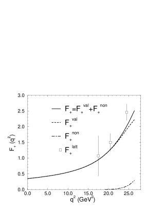
Figure 21: The $B\to\pi$ form factor $F_{+}$ compared with the lattice QCD results [210].

Assume some model wave functions, whose parameters can be fixed from the quark masses, decay constants, and other experimental data [205]. The numerical results of the $B\to\pi$ form factor $F_{+}$ are ploted in Fig. 21. The form factor values are consistent with those obtained in the $q^{+}=0$ frame followed by an anatylic continuation to the time-like region [211]. It is found that the nonvalence contribution to heavy-to-light transitions is negligible in the whole region of $q^{2}$ except near zero recoil ($q^{2}\sim q^{2}_{\rm max}$). In addition, for the same final meson, the nonvalence contributions are smaller when the inital mesons are heavier. This conclusion is consistent with those drawn in [194, 198, 202, 203].

Figure 22: Non-wave-function vertex(black blob) linked to an ordinary LF wave function(white blob).

Another treatment of the nonvalence state is to adopt the Schwinger-Dyson equation, which connects the embedded state (the black blob in Fig. 22) to the ordinary light-cone wave function (white blob in Fig. 22) [206]. This connection from one-body to three-body sector can be achieved by introducing an operator ${\cal K}$, which in general depends on the involved momenta. It is easy to see that the following link between the non-wave-function vertex (black blob) and the ordinary LF wave function (white blob) naturally arises,

$$(M^{2}-M^{\prime 2}_{0})\Psi^{\prime}(x_{i},{\bf k}_{Ti})=\int[dy][d^{2}{\bf l}_{T}]{\cal K}(x_{i},{\bf k}_{Ti};y_{j},{\bf l}_{Tj})\Psi(y_{j},{\bf l}_{Tj})\;,$$ (138)

where $M$ is the mass of outgoing meson and $M^{\prime 2}_{0}=(m^{2}_{1}+{\bf k}^{2}_{T1})/x_{1}-(m^{2}_{2}+{\bf k}^{2}_{T2})/(-x_{2})$ with $x_{1}=1-x_{2}>1$ due to the kinematics of the non-wave-function vertex. Note that Eq. (138) essentially takes the same form as the LF bound-state equation.

Figure 23: Effective calculation of the embedded state (black blob) in terms of the usual LC wave fucntion (white blob).

Next step is to remove the four-body energy denomenator $D_{4}$ using the identity,

$$\frac{1}{D_{4}D^{g}_{2}}+\frac{1}{D_{4}D^{h}_{2}}=\frac{1}{D^{g}_{2}D^{h}_{2}}\;.$$ (139)

One then obtains the amplitude identical to the nonvalence contribution in terms of ordinary LF wave functions of gauge boson and hadron (white blob) as shown in Fig. 23(d). Hence, the valence and nonvalence contributions can be calculated by menas of the ordinary LF wave functions with the latter involving an unknown operator $\cal K$. It has been argued that the right-hand side of Eq. (138) can be approximated as a constant for heavy meson decays in the region with small momentum transfer [206]. In contact interaction case, it has been verified that the prescription of a constant operator in Fig. 23(d) is an exact solution of Fig. 23(a). The above formalism has been applied to the $D\to K$ transition form factors [206].

5 Two-Body Nonleptonic Decays

In this section I review progress on the understanding of QCD dynamics in two-body charmless nonleptonic $B$ meson decays. Topics related to charmed decays will be arranged in the next section. Intuitively, decay products from the heavy $b$ quark move fast without further interaction between them. This simple picture, supported by the color-transparency argument [67], leads to the naive factorization. Although the factorization assumption (FA) [212] gives predictions in relatively good agreement with data (apart from the color-suppressed modes), it provides no insight into dynamics. Moreover, FA suffers serious theoretical drawbacks as explained below. To improve FA, several frameworks, based on different assumptions of the dominant dynamics in exclusive $B$ meson decays, have been developed. Amomg these, I will discuss the QCDF, PQCD and LCSR approaches.

5.1 Factorization Assumption

To explain the idea of FA, I take the decay $\bar{B}^{0}\to D^{+}\pi^{-}$ as an example. The relevant effective weak Hamiltonian is given by

$${\cal H}_{\rm eff}={G_{F}\over\sqrt{2}}\,V_{cb}V_{ud}^{*}\Big{[}C_{1}(\mu)O_{1}(\mu)+C_{2}(\mu)O_{2}(\mu)\Big{]}\;,$$ (140)

with the four-fermion operatos,

$$O_{1}=(\bar{d}b)_{{}_{V-A}}(\bar{c}u)_{{}_{V-A}}\;,\qquad\qquad O_{2}=(\bar{c}b)_{{}_{V-A}}(\bar{d}u)_{{}_{V-A}},$$ (141)

and the definition $(\bar{q}_{1}q_{2})_{{}_{V\pm A}}\equiv\bar{q}_{1}\gamma_{\mu}(1\pm\gamma_{5})q_{2}$. To ensure the renormalization-scale and -scheme independences of physical amplitudes, the matrix elements of four-fermion operators have to be evaluated in the same renormalization scheme as that for Wilson coefficients and renormalized at the same scale $\mu$. Under FA, the matrix element $\langle O(\mu)\rangle$ is factorized into the product of two matrix elements of single currents, governed by decay constants and form factors. The naive factorization was first proved in the framework of large energy effective theory [181], and justified in the large $N_{c}$ limit [213]. For nice reviews, refer to [214].

In spite of its simplicity, FA encounters three principal difficulties. First, the hadronic matrix element under FA is independent of the renormalization scale $\mu$, as the vector or axial-vector current is partially conserved. Consequently, the amplitude $C_{i}(\mu)\langle O\rangle_{\rm fact}$ is not truly physical as the scale dependence of Wilson coefficients does not get compensation from the matrix elements. Second, nonfactorizable contributions have been neglected. This may be the reason FA fails to describe the color-suppressed decays, such as $B\to J/\psi K^{(*)}$. Strong phases are essential for predicting CP asymmetries in exclusive $B$ meson decays. These phases, arising from the Bander-Silverman-Soni (BSS) mechanism [215], are ambiguous in FA. In this mechanism the $c$ quark loop contributes an imaginary piece proportional to,

$$C_{2}(t)\alpha_{s}(t)\int duu(1-u)\theta(q^{2}u(1-u)-m_{c}^{2})\;,$$ (142)

where $q^{2}$ is the invariant mass of the gluon emitted from the penguin. Since $q^{2}$ is not clearly defined in FA, one can not obtain definite information of the strong phase from Eq. (142).

The scale problem in FA can be circumvented in two prescriptions. First, one incorporates nonfactorizable effects into the effective coefficients [216, 217, 218]:

$$a_{1}^{\rm eff} = C_{2}(\mu)+C_{1}(\mu)\left[{1\over N_{c}}+\chi_{1}(\mu)\right]\,,$$

$$a_{2}^{\rm eff} = C_{1}(\mu)+C_{2}(\mu)\left[{1\over N_{c}}+\chi_{2}(\mu)\right]\,,$$ (143)

where nonfactorizable terms are characterized by the parameters $\chi_{i}$. The $\mu$ dependence of Wilson coefficients is assumed to be exactly compensated by that of $\chi_{i}(\mu)$ [214]. However, the renormalized four-fermion operator by itself still depends on $\mu$, though the scale dependence of $\langle O(\mu)\rangle$ is lost in FA. To next-to-leading order, the Wilson coefficients depend on the choice of the renormalization scheme, and it is not clear if $\chi_{i}(\mu)$ can restore the scheme independence of the matrix element.

In the second prescription, $\langle O(\mu)\rangle$ is related to the tree-level hadronic matrix element via the relation $\langle O(\mu)\rangle=g(\mu)\langle O\rangle_{\rm tree}$. The factor $g(\mu)$ is obtained by calculating loop corrections to the weak decay vertices. Then schematically one writes

$$C(\mu)\langle O(\mu)\rangle=C(\mu)g(\mu)\langle O\rangle_{\rm tree}\equiv C^{\rm eff}\langle O\rangle_{\rm tree}.$$ (144)

FA is applied afterwards to the hadronic matrix element of the operator $O$ at the tree level. Since the tree-level matrix element $\langle O\rangle_{\rm tree}$ is renormalization scheme and scale independent, so are the effective Wilson coefficients $C_{i}^{\rm eff}$ and the effective parameters $a_{i}^{\rm eff}$ expressed by [219, 220]

$$a_{1}^{\rm eff} = C_{1}^{\rm eff}+C_{2}^{\rm eff}\left({1\over N_{c}}+\chi_{1}\right)\,,$$

$$a_{2}^{\rm eff} = C_{2}^{\rm eff}+C_{1}^{\rm eff}\left({1\over N_{c}}+\chi_{2}\right)\,.$$ (145)

Unfortunately, the extraction of $g(\mu)$ from the matrix element is infrared divergent. The divergences are usually regularized by considering off-shell momenta $p$ for the external quark lines with $p^{2}<0$. What one has achieved is actually

$$C^{\rm eff}=C(\mu)g(\mu,-p^{2},\lambda)\;,$$ (146)

with $p^{2}$ being the infrared cutoff, and $\lambda$ a gauge parameter. Obviously, $c^{\rm eff}$ is subject to the ambiguities of the infrared cutoff and the gauge dependence. As stressed in [221], the gauge and infrared dependences always appear as long as the matrix elements are evaluated between quark states. The reason has been implicitly pointed out in [222] that “off-shell renormalized vertices of gauge-invariant operators are in general gauge dependent”. Also, the nonfactorizable contributions are included by introducing more free parameters as shown in Eq. (145). These parameters, being process-dependent, then make FA even less predictive. The difficulty in predicting strong phases in FA also remains.

5.2 QCD Factorization

An important step towards a rigorous framework for two-body nonleptonic $B$ meson decays in the heavy quark limit has been made [23, 69, 223]. The infrared divergences appearing in the loop corrections to the weak deacy vertices are absorbed into a $B$ meson transition form factor, such that $g(\mu)$ can be evaluated in terms of on-shell external quarks. In this way, the infrared divergences are regularized without breaking the gauge invariance. The nonfactorizable contribution is calculated in the framework of collinear factorization theorem, since it is not suffered by the end-point singularity at least at leading twist due to the color-transparency argument. The gluon invariant mass $q^{2}$ in the BSS mechanism can be clearly defined and related to parton momentum fractions in collinear factorization theorem. Therefore, the theoretical difficulties in FA are resolved in principle in this QCDF approach.

Figure 24: Graphic representation of QCD factorization

The resulting factorization formula for the decay amplitudes incorporates elements both of FA sketched above and of the hard-scattering picture. Consider a decay $B\to M_{1}M_{2}$, where $M_{1}$ picks up the spectator quark. If $M_{1}$ is either a heavy ($D$) or a light ($\pi$, $K$) meson, and $M_{2}$ a light ($\pi$, $K$) meson, QCDF gives the following structure,

$$A(B\to M_{1}M_{2})=\left[\mbox{``naive factorization''}\right]\times\left[1+O(\alpha_{s})+O(\Lambda_{\rm QCD}/m_{b})\right]\;.$$ (147)

The $O(\alpha_{s})$ term contains the finite piece of the loop corrections to the decay vertices and the nonfactorizable contributions. The $O(\Lambda_{\rm QCD}/m_{B})$ term collects the power corrections to FA, such as those from the annihilation topology. Both terms are supposed to be calculable in a systematic way in QCDF. Equation (147), without the chirally enhanced twist-3 contributions, has been proved to all orders in $\alpha_{s}$ in the framework of SCET [224].

The leading term in $1/m_{b}$ is then written, according to Eq. (147), as

$$\langle M_{1}M_{2}|O_{i}|\bar{B}\rangle = F^{BM_{1}}(0)\int_{0}^{1}\!\!du\,T^{I}(u)\phi_{M_{2}}(u)$$ (148)

$$+\!\int\!d\xi dudv\,T^{II}(\xi,u,v)\,\phi_{B}(\xi)\phi_{M_{1}}(v)\phi_{M_{2}}(u)\;,$$

which is graphically described in Fig. 24. $F^{BM_{1}}$ is a nonperturbative form factor, and $\phi_{M_{i}}$ and $\phi_{B}$ the light-cone distribution amplitudes. The hard kernel $T^{I}$ absorbs the finite part of the loop corrections to the decay vertices. The hard kernel $T^{II}$ corresponds to the nonfactorizable contributions. It is easy to find that Eq. (148) is similar to the leading-power QCDF expression for a $B$ meson transition form factor in Eq. (113).

For QCDF, the universal nonperturbative inputs include not only hadron distribution amplitudes, but also $B$ meson transition form factors. It has been found that the end-point singularities exist in the twist-3 factorization formula for the nonfactorizable amplitudes, and in power-suppressed annihilation amplitudes. Because of these end-point singularities, the $O(\alpha_{s})$ and $O(\Lambda_{\rm QCD}/m_{B})$ terms in Eq. (147) turn out to be uncalculable, and their contributions have been parametrized into

$$\ln\frac{m_{B}}{\Lambda}\left(1+\rho_{H}e^{i\delta_{H}}\right)\;,\;\;\;\;\ln\frac{m_{B}}{\Lambda}\left(1+\rho_{A}e^{i\delta_{A}}\right)\;,$$ (149)

respectively. In fact, the singularities signal the breakdown of factorization. QCDF then contains the non-universal and uncontrollable parameters $\rho_{H,A}$ and $\delta_{H,A}$. These arbitrary parameters can be determined, together with the unitarity angles, from the best fit to experimental data [223, 225]. To make predictions, QCDF usually presents large theoretical uncertainty due to the arbitrary parameters. Another source of theoretical uncertainty comes from the scalar currents, which are proportional to the chiral symmetry breaking scale $m_{0}=m_{\pi}^{2}/(m_{u}+m_{d})$ [23].

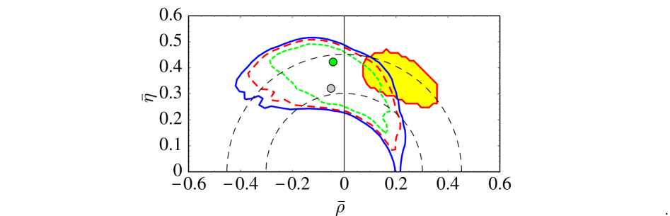
Figure 25: 95% (solid), 90% (dashed) and 68% (short-dashed) confidence level contours in the $(\bar{\rho},\bar{\eta})$ plane obtained from a global fit to the CP averaged $B\to\pi\pi,K\pi$ branching ratios. The darker dot shows the overall best fit, whereas the lighter dot indicates the best fit for the default hadronic parameter set. The light-shaded region indicates the region preferred by the standard global fit [35], including the direct measurement of $\sin(2\phi_{1})$.

It is possible to extract the unitarity angle $\phi_{3}$ from the data of the CP-averaged $B\to\pi\pi$ and $B\to K\pi$ branching ratios. The global fit of the Wolfenstein parameters $(\bar{\rho},\bar{\eta})$ to the six measured $B\to\pi\pi,K\pi$ world-averaged branching ratios is displayed in Fig. 25 [227]. The best fits with theory parameters in the allowed ranges [223] have $\chi^{2}\approx 0.5$. The ranges of the strange quark mass and of the $B$ meson decay constant are $[75,125]\,\mbox{MeV}$ and $[170,230]\,\mbox{MeV}$, respectively. Since a wide range of $\phi_{3}$ is allowed, the result is consistent with the standard fit based on meson mixing and $|V_{ub}|$. Figure 25 shows a preference for $\phi_{3}$ slightly greater than $90^{\circ}$. This result is similar to that from a fit based on naive FA [226].

Decay Mode	Exp. Average	Default fit	Fit2
$B^{0}\to\pi^{+}\pi^{-}$	$5.15\pm 0.61$	5.12	5.24
$B^{\pm}\to\pi^{\pm}\pi^{0}$	$4.88\pm 1.06$	5.00	4.57
$B^{0}\to\pi^{0}\pi^{0}$	$-$	0.78	0.94
$B^{0}\to\ K^{\pm}\pi^{\mp}$	$18.56\pm 1.08$	17.99	18.47
$B^{\pm}\to K^{\pm}\pi^{0}$	$11.49\pm 1.26$	12.07	11.83
$B^{\pm}\to K^{0}\pi^{\pm}$	$17.93\pm 1.70$	15.65	17.88
$B^{0}\to K^{0}\pi^{0}$	$8.82\pm 2.20$	5.55	6.87

Table 4: CP-averaged $B\to\pi\pi,K\pi$ branching ratios (in units of $10^{-6}$): data vs. results from the fits. The default fit to $(\bar{\rho},\bar{\eta})$ (returning $|V_{ub}/V_{cb}|=0.085$, $\phi_{3}=116^{\circ}$ with $\chi^{2}=4.5$) refers to the default theory parameter set used in [223]. “Fit2” (returning $|V_{ub}/V_{cb}|=0.079$, $\phi_{3}=97^{\circ}$, $\chi^{2}=1.0$) refers to a fit without annihilation contributions and chirally enhanced spectator corrections.

The experimental data and QCDF fits are presented in Table 4 [227]. The last two columns come from the fitted branching ratios for the default theory parameter set in [223] and the central values of the above ranges for $m_{s}$ and $f_{B}$, and for a second set, where all annihilation effects and chirally enhanced spectator interactions are removed. The second set also leads to a good fit without these uncertain power-suppressed effects. The normalization of the $B\to K\pi$ modes are sensitive to weak annihilation and to the strange quark mass through the scalar penguin amplitude. If $\phi_{3}$ is assumed to take values around $55^{\circ}$ as favored by indirect constraints, the agreement becomes worse for the branching ratios with significant tree and penguin interference. Note that the inclusion of the annihilation contribution weakens the constraint from nonleptonic $B$ meson decays on a global fit of $\phi_{3}$ [36, 228].

The direct and mixing-induced CP asymmetries in the $B_{d}^{0}\to\pi^{+}\pi^{-}$ decay are also the important quantities for extracting the unitarity angles. The time-dependent asymmetry is defined as

$$A(t) \equiv {\Gamma(\bar{B}^{0}(t)\to\pi^{+}\pi^{-})-\Gamma(B^{0}(t)\to\pi^{+}\pi^{-})\over\Gamma(\bar{B}^{0}(t)\to\pi^{+}\pi^{-})+\Gamma(B^{0}(t)\to\pi^{+}\pi^{-})}\;,$$ (150)

$$= S_{\pi\pi}\,\sin(\Delta mt)-C_{\pi\pi}\,\cos(\Delta mt)\;,$$

where the direct and mixing-induced asymmetries,

$$C_{\pi\pi}={1-|\lambda_{\pi\pi}|^{2}\over 1+|\lambda_{\pi\pi}|^{2}}\;,\hskip 56.9055ptS_{\pi\pi}={2\,Im(\lambda_{\pi\pi})\over 1+|\lambda_{\pi\pi}|^{2}}\;,$$ (151)

respectively, satisfy the relation $C_{\pi\pi}^{2}+S_{\pi\pi}^{2}\leq 1$. The factor $\lambda_{\pi\pi}$ is given by

$$\lambda_{\pi\pi}=|\lambda_{\pi\pi}|\,e^{2i(\phi_{2}+\Delta\phi_{2})}=e^{2i\phi_{2}}\left[{1+R_{c}e^{i\delta}\,e^{i\phi_{3}}\over 1+R_{c}e^{i\delta}\,e^{-i\phi_{3}}}\right]\;,$$ (152)

with the penguin-over-tree ratio $R_{c}=|P/T|$ and the strong phase difference between penguin and tree amplitudes, $\delta=\delta_{P}-\delta_{T}$. We have $S_{\pi\pi}=\sin(2\phi_{2})$, if the penguin amplitude is zero.

The predicted correlation between $S_{\pi\pi}$ and $C_{\pi\pi}$ from QCDF is shown in Fig. 26 [227], where the $B\bar{B}$ mixing phase has been fixed to $\sin(2\phi_{1})=0.78$. Each closed curve is generated by specifying the theory input and varying $\phi_{3}$ from 0 to $360^{\circ}$. The central (dark) curve refers to the calculation of $P/T$ with the default theory parameter set, the two neighboring (lighter) curves refer to $P/T$ plus-minus its theoretical error without the error from weak annihilation (but including the one from $|V_{ub}|$), and the final (lightest) curves also include the error from weak annihilation. The black part on each curve marks the point $\phi_{3}=60^{\circ}$; the fat line segment marks the range $[40^{\circ},80^{\circ}]$ favored by the standard unitarity triangle fit with larger $\phi_{3}$ to the right of the black part. Note that the Belle data [229] are close to the boundary of the physical region.

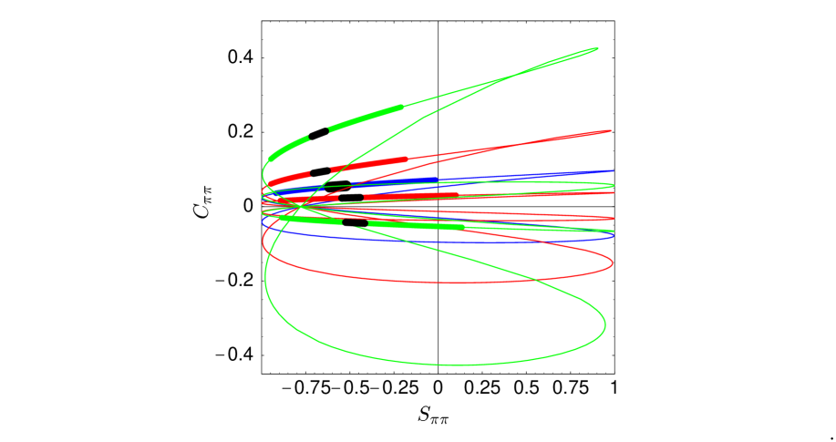
Figure 26: Predicted correlation between the mixing-induced and direct CP asymmetries in the $B_{d}\to\pi^{+}\pi^{-}$ decay. See text for explanation of the different curves.

The recent BaBar measurement [230] with $90\%$ C.L. interval, taking into account the systematic errors, are

$$S_{\pi\pi}=0.02\pm 0.34\pm 0.05\;, [-0.54,\hskip 14.22636pt+0.58]\;,$$ (153)

$$C_{\pi\pi}=-0.30\pm 0.25\pm 0.04\;, [-0.72,\hskip 14.22636pt+0.12]\;.$$

It is observed that the QCDF predictions prefer a small $C_{\pi\pi}$, which are close to the upper bound of the BaBar data. The predictions for $S_{\pi\pi}$ depend on $\phi_{2}$. The determination of the CKM matrix elements from the measurement of $S_{\pi\pi}$ in the QCDF framework has been performed in [231].

Mode	Default	$m_{s}=80$ MeV	$F_{2}=0.1$	Experiment
$B^{-}\to K^{-}\eta^{\prime}$	$42_{\,-12\,-11}^{\,+16\,+27}$	$59_{\,-16\,-17}^{\,+22\,+41}$	$56_{\,-14\,-13}^{\,+19\,+31}$	$72.2\pm 5.3$
$\bar{B}^{0}\to\bar{K}^{0}\eta^{\prime}$	$41_{\,-11\,-11}^{\,+15\,+26}$	$57_{\,-15\,-16}^{\,+21\,+39}$	$56_{\,-13\,-13}^{\,+18\,+30}$	$54.8\pm 10.1$
$B^{-}\to K^{-}\eta$	$1.7_{\,-1.5\,-0.5}^{\,+2.0\,+1.3}$	$2.2_{\,-2.0\,-0.8}^{\,+2.7\,+1.9}$	$1.4_{\,-1.2\,-0.5}^{\,+1.8\,+1.1}$	$<6.9$
$\bar{B}^{0}\to\bar{K}^{0}\eta$	$1.0_{\,-1.2\,-0.4}^{\,+1.7\,+1.1}$	$1.4_{\,-1.7\,-0.6}^{\,+2.4\,+1.6}$	$0.7_{\,-0.9\,-0.4}^{\,+1.5\,+0.9}$	$<9.3$
$B^{-}\to K^{-}\pi^{0}$	$9.4_{\,-2.9\,-2.4}^{\,+3.2\,+5.6}$	$12.6_{\,-3.8\,-3.5}^{\,+4.3+8.2}$	$9.4_{\,-2.9\,-2.4}^{\,+3.2\,+5.6}$	$12.7\pm 1.2$
$\bar{B}^{0}\to\bar{K}^{0}\pi^{0}$	$5.9_{\,-2.3\,-1.9}^{\,+2.7\,+4.5}$	$8.5_{\,-3.1\,-2.8}^{\,+3.7\,+6.8}$	$5.9_{\,-2.3\,-1.9}^{\,+2.7\,+4.5}$	$10.2\pm 1.5$
$B^{-}\to K^{*-}\eta^{\prime}$	$3.5_{\,-3.7\,-1.7}^{\,+4.4\,+4.7}$	$7.7_{\,-6.7\,-3.2}^{\,+7.6\,+8.0}$	$2.7_{\,-2.6\,-1.3}^{\,+3.5\,+3.9}$	$<35$
$\bar{B}^{0}\to\bar{K}^{*0}\eta^{\prime}$	$2.5_{\,-3.1\,-1.5}^{\,+3.8\,+4.3}$	$6.3_{\,-5.8\,-2.9}^{\,+6.8\,+7.4}$	$1.2_{\,-1.8\,-0.9}^{\,+2.7\,+3.2}$	$<13$
$B^{-}\to K^{*-}\eta$	$8.6_{\,-2.6\,-\phantom{1}4.4}^{\,+3.0\,+14.0}$	$13.8_{\,-4.2\,-\phantom{1}6.7}^{\,+4.8\,+19.8}$	$9.1_{\,-2.7\,-\phantom{1}4.6}^{\,+3.1\,+14.3}$	$26.5\pm 6.1$
$\bar{B}^{0}\to\bar{K}^{*0}\eta$	$8.7_{\,-2.6\,-\phantom{1}4.5}^{\,+2.9\,+14.0}$	$13.9_{\,-4.1\,-\phantom{1}6.7}^{\,+4.6\,+19.5}$	$9.2_{\,-2.7\,-\phantom{1}4.7}^{\,+3.0\,+14.2}$	$16.4\pm 3.0$
$B^{-}\to K^{*-}\pi^{0}$	$3.2_{\,-1.1\,-1.3}^{\,+1.2\,+4.0}$	$3.3_{\,-1.2\,-1.5}^{\,+1.3\,+4.8}$	$3.2_{\,-1.1\,-1.3}^{\,+1.2\,+4.0}$	$<31$
$\bar{B}^{0}\to\bar{K}^{*0}\pi^{0}$	$0.7_{\,-0.5\,-0.6}^{\,+0.6\,+2.4}$	$0.7_{\,-0.5\,-0.6}^{\,+0.6\,+3.0}$	$0.7_{\,-0.5\,-0.6}^{\,+0.6\,+2.4}$	$<3.6$

Table 5: Predictions for the CP-averaged branching ratios (in units of $10^{-6}$), assuming $\phi_{3}=70^{\circ}$, $|V_{cb}|=0.041$ and $|V_{ub}/V_{cb}|=0.09$. The first error is due to parameter variations, and the second one shows the estimate of the uncertainty due to weak annihilation. The column labeled “default” refers to $m_{s}=100$ MeV and $F_{2}=0$.

The QCDF formalism has been extended to the study of $B\to VP$ modes [232, 233, 234, 235]. The $B\to\phi K$ branching ratios were predicted to be around $4\times 10^{-6}$ [232, 233], which seems to be smaller than the experimental data (see Table 7). The reason is that the same set of free parameters in Eq. (149) has been adopted for the $B\to PP$ and $VP$ decay amplitudes. The annihilation contribution is then constrained by the $B\to K\pi$ branching ratios, and can not help to increase the $B\to\phi K$ branching ratios. In a global fit performed in [234] these parameters have been assumed to be different for the $B\to PP$ and $VP$ modes. Introducing two independent sets of free parameters, the $B\to\phi K$ branching ratios can be fit (due to a larger annihilation contribution) without increasing the $B\to K\pi$ ones. However, the data for the $B\to K^{*}\pi$ modes were not included into the global fit. It has been noticed [235] that once the $B\to K^{*}\pi$ modes are included, the confidence level of the best fit drops to below 0.1%. The possible large direct CP asymmetry in the $B\to\rho\pi$ decays [236] also deteriorate the fit.

QCDF has been also applied to flavor-singlet $B$ meson decays, such as $B\to K^{(*)}\eta^{(\prime)}$ [237]. It is difficult to account for the branching ratios of these modes in FA [238]. The scheme for the $\eta$-$\eta^{\prime}$ mixing, with a single mixing angle advocated in [239], was assumed. The contributions from the $b\to c\bar{c}s$ and $b\to sgg$ transitions through the gluon content of singlet mesons were analyzed carefully. Also, a singlet annihilation amplitude, where two gluons radiating from the spectator quark form an $\eta^{(\prime)}$ meson, contributes at leading power. The unknown form factors $F_{0}^{B\eta^{(\prime)}}(0)$ were parametrized as

$$F_{0}^{BP}(0)=F_{1}\,\frac{f_{P}^{q}}{f_{\pi}}+F_{2}\,\frac{\sqrt{2}f_{P}^{q}+f_{P}^{s}}{\sqrt{3}f_{\pi}}\,,$$ (154)

with $P=\eta$ or $\eta^{\prime}$ and $q=u$, $d$. The decay constants $f_{P}^{q}$ and $f_{P}^{s}$ are defined through the quark currents. In [237] $F_{1}=F_{0}^{B\pi}(0)$ and $F_{2}=0$ or 0.1 were adopted. Combining the above effects, the predictions for the CP-averaged $B\to K^{(*)}(\eta^{(\prime)},\pi^{0})$ branching ratios from QCDF are summarized in Table 5.

5.3 Perturbative QCD

As stated before, the PQCD approach to two-body nonleptonic $B$ meson decays is based on $k_{T}$ factorization. Therefore, the theoretical difficulties in FA can also be resolved but in a way different from that of QCDF. The infrared divergences appearing in the loop corrections to the weak deacy vertices are absorbed into meson wave functions, such that the infrared divergences are regularized without breaking the gauge invariance. The factorizable, nonfactorizable and power-suppressed annihilation contributions are calculated in the framework of $k_{T}$ factorization theorem without the end-point singularities. The arbitrary cutoffs introduced in QCDF [69, 223] are not necessary, and PQCD involves only universal and controllable inputs. The gluon invariant mass $q^{2}$ in the BSS mechanism can also be clearly defined and related to parton momentum fractions.

Figure 27: Factorization of two-body nonleptonic $B$ meson decays in the PQCD approach.

The amplitude for the $B\to M_{1}M_{2}$ decay is then factorized into the convolution of the six-quark hard kernel, the Wilson coefficient, the jet function and the Sudakov factor with the bound-state wave functions as shown in Fig. 27 [240, 241, 242, 243],

$$A=\phi_{B}\otimes H^{(6)}\otimes J\otimes S\otimes\phi_{M_{1}}\otimes\phi_{M_{2}}\;,$$ (155)

all of which are well-defined and gauge-invariant. $J$ denotes the jet function from threshold resummation discussed in Sec. 2.3, and $S$ denotes the Sudakov factor from $k_{T}$ resummation discussed in Sec. 3.3. $J$ ($S$), organizing the double logarithms in the hard kernel (meson wave functions), is hidden in $H$ (the three meson states) in Fig. 27. The partition of nonperturbative and perturbative contributions is quite arbitrary. Different partitions correspond to different factorization schemes. However, the decay amplitude, as the convolution of the above factors, is independent of factorization schemes as it should be.

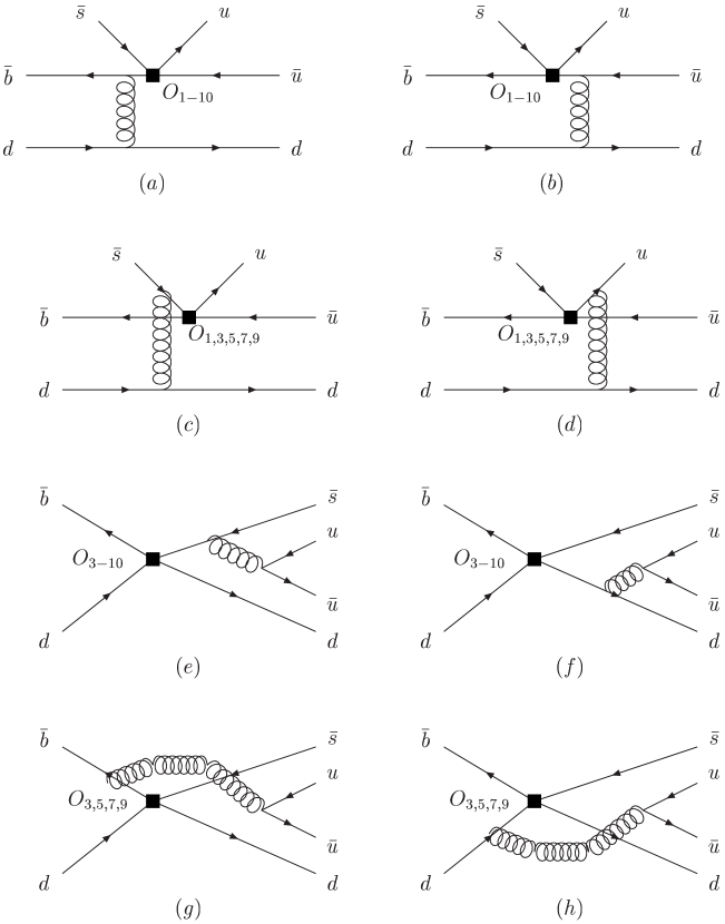
Figure 28: Leading-order diagrams for the six-quark hard kernel in the PQCD approach.

The six-quark hard kernel $H^{(6)}$ consists of the diagrams with at least one hard gluon [244]. The complete set of leading-order diagrams for the $B\to K\pi$ decays is displayed in Fig. 28. Figures 28(a) and 28(b), referred to as the factorizable emission, correspond to the leading contribution in QCDF [the left-hand diagram in Fig. 24]. Figures 28(c) and 28(d), referred to as the nonfactorizable emission, correspond to the next-to-leading-order contribution in QCDF [the right-hand diagram in Fig. 24]. Figures 28(e) and 28(f), and Figs. 28(g) and 28(h) are referred to as the factorizable annihilation and the nonfactorizable annihilation, respectively. They are explicitly power-suppressed. However, for the physical mass $m_{B}\sim 5$ GeV, the scalar contribution from the penguin operators, proportional to $m_{0}/m_{B}$, is not really negligible.

Figure 29: (a) The factorizable emission amplitude as a function of $m_{B}$ in unit of GeV. (b) The ratio $r$ of the nonfactorizable emission amplitude over the factorizable one as a function of $m_{B}$.

The factorization limit of the PQCD approach at large $m_{B}$, which is not as obvious as in QCDF, has been examined [245]. It was found that the factorizable emission amplitude in Figs. 28(a) and 28(b) decreases like $m_{B}^{-3/2}$ as displayed in Fig. 29(a), if the $B$ meson decay constant $f_{B}$ scales like $f_{B}\propto m_{B}^{-1/2}$. This power-law behavior is consistent with that obtained in [69, 18]. Define $r$ as the ratio of the magnitude of the nonfactorizable emission amplitude [from Figs. 28(c) and 28(d)] over the factorizable one. Figure 29(b), exhibiting $r$ as a function of $m_{B}$, indicates that the curve actually descends with $m_{B}$ despite of small oscillation. If parametrizing the ratio as

$$r\equiv\frac{|\rm Nonfact.|}{\rm Fact.}\propto\frac{1}{\ln^{\alpha}(m_{B}/\Lambda)}\;,$$ (156)

the best fit to the curve gives the power $\alpha\sim 1.0$ for $\Lambda\sim 0.4$ GeV [245]. This logarithmic decrease has been confirmed up to $m_{B}=300$ GeV. It implies that the PQCD formalism approaches FA logarithmically.

Surprisingly, the behavior of the ratio $r$ with $m_{B}$ in PQCD is close to that in QCDF. However, the reasonings for achieving the same power counting are quite different. In QCDF the factorizable contribution is assumed to be dominated by soft dynamics, and identified as being of $O(\alpha_{s}^{0})$. The nonfactorizable contribution, being calculable, starts from $O(\alpha_{s})$. Because of the soft cancellation at $x_{3}\sim O(\Lambda/m_{B})$, the nonfactorizable emission amplitude is dominated by the contribution from the region with $x_{3}\sim O(1)$. In this region there is no further power suppression, and one has the ratio,

$$r_{\rm QCDF}\sim\alpha_{s}(m_{B})\propto\frac{1}{\ln(m_{B}/\Lambda_{\rm QCD})}\;.$$ (157)

In PQCD based on $k_{T}$ factorization theorem [95, 96], both the factorizable and nonfactorizable contributions, being calculable, start from $O(\alpha_{s})$. However, the Sudakov factor modifies the factorization formulas in the way that a pair of nonfactorizable diagrams exhibits a stronger cancellation as $m_{B}$ increases [246]. It turns out that the ratio $r$ also vanishes logarithmically as shown in Eq. (156).

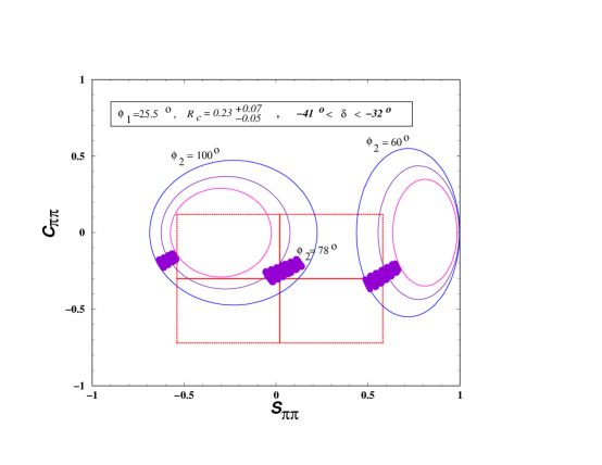
Figure 30: Plot of $C_{\pi\pi}$ vs $S_{\pi\pi}$ for various values of $\phi_{2}$ with $\phi_{1}=25.5^{o}$, $0.18<R_{c}<0.30$ and $-41^{o}<\delta<-32^{o}$ in PQCD. The allowed experimental ranges from BaBar measurment within $90\%$ C.L. was considered. Dark areas are the regions allowed by PQCD for different $\phi_{2}$.

I then discuss the applications of PQCD to two-body nonleptonic $B$ meson decays. An alternative way to determine $\phi_{2}$ is to use the time-dependent CP asymmetry in the $B_{d}^{0}(t)\to\pi^{+}\pi^{-}$ decay, which provides two constraints from $C_{\pi\pi}$ and $S_{\pi\pi}$ for three unknown variables $R_{c},\delta$ and $\phi_{2}$ in Eq. (150). If one knows $R_{c}$ and $\delta$, $\phi_{2}$ can be extracted from the experimental data of $C_{\pi\pi}$ vs $S_{\pi\pi}$. Since PQCD gives $R_{c}=0.23^{+0.07}_{-0.05}$ and $-41^{o}<\delta<-32^{o}$, the allowed range of $\phi_{2}$ at present stage has been fixed to be $55^{o}<\phi_{2}<100^{o}$ as shown in Fig. 30 [247]. Because the strong phase in PQCD is relatively large compared to that in QCDF as explained below, a significant direct CP asymmetry $C_{\pi\pi}=-(23\pm 7)\%$ was predicted, which could be tested by more precise experimental measurement in the near future [1, 248]. The central point of the BaBar data in Eq. (153) [230] then corresponds to $\phi_{2}=78^{o}$. Denote $\Delta\phi_{2}$ as the uncertainty of $\phi_{2}$ due to the penguin contribution. For the allowed region of $\phi_{2}=(55\sim 100)^{o}$, one obtains $\Delta\phi_{2}=(8\sim 16)^{o}$, implying sizable penguin contributions in the $B_{d}^{0}\to\pi^{+}\pi^{-}$ decay. The main uncertainty comes from the value of $|V_{ub}|$.

Here I give a simple explanation for the different phenomenological consequences of the CP asymmetries in two-body nonleptonic $B$ meson decays derived from QCDF and from PQCD. According to the QCDF power counting rules [23, 69] based on collinear factorization, the factorizable emission diagram gives the leading contribution of $O(\alpha_{s}^{0})$, since the $B\to\pi$ form factor is not calculable. Because the leading contribution is real, the strong phase arises from the factorizable annihilation diagram, being of $O(\alpha_{s}m_{0}/m_{B})$, and from the vertex correction to the leading diagram, being of $O(\alpha_{s})$. For $m_{0}/m_{B}$ slightly smaller than unity, the vertex correction is the leading source of strong phases. In $k_{T}$ factorization the power counting rules change [246]. The factorizable emission diagram is calculable and of $O(\alpha_{s})$. The factorizable annihilation diagram has the same power counting as in QCDF. The vertex correction becomes of $O(\alpha_{s}^{2})$. Therefore, the annihilation diagram contributes the leading strong phase. This is the reason the strong phase derived from PQCD and from QCDF could be opposite in sign, and the former has a large magnitude. As a consequence of the different power counting rules, QCDF prefers a small and positive CP asymmetry $C_{\pi\pi}$ [227], while PQCD prefers a large and negative $C_{\pi\pi}$ [26, 247, 249, 250, 251]. Significant CP asymmetries are also expected in the $B\to K\pi$ [25], $B\to KK$ [252] and $B\to\rho K$, $\omega K$ [253] decays. The last two modes are especially sensititve to the annihilation contributions.

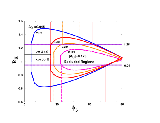
Figure 31: Plot of $R_{K}$ vs $\phi_{3}$ with $r_{K}=0.164,0.201$ and $0.238$.

The CP-averaged $B\to K\pi$ branching ratios may lead to nontrivial constaints on the angle $\phi_{3}$ [6, 7]. Introduce the observables,

$$R_{K} = {{Br}(B^{0}\to K^{\pm}\pi^{\mp})\,\,\tau_{+}\over{Br}(B^{\pm}\to K^{0}\pi^{\pm})\,\,\tau_{0}}\;,$$

$$A_{0} = A_{CP}(B^{0}\to K^{+}\pi^{-})\,\,R_{K}\;,$$ (158)

with the tree-over-penguin ratio $r_{K}=|T^{{}^{\prime}}/P^{{}^{\prime}}|$ for the $B\to K\pi$ decays, and the strong phase difference between the tree and penguin amplitides, $\delta=\delta_{T^{\prime}}-\delta_{P^{\prime}}$. One has [247]

$$R_{K}=1+r_{K}^{2}\pm\sqrt{4r_{K}^{2}\cos^{2}\phi_{3}-A_{0}^{2}\cot^{2}\phi_{3}}\;,$$ (159)

with $r_{K}=0.201\pm 0.037$ from PQCD [25], and $A_{0}=-0.110\pm 0.065$ from the recent BaBar measurement $A_{CP}(B_{d}^{0}\to K^{+}\pi^{-})=-10.2\pm 5.0\pm 1.6\%$ [230] and the present world-averaged value of $R_{K}=1.10\pm 0.15$ [254].

With the values $\delta_{P^{\prime}}=157^{o}$, $\delta_{T^{\prime}}=1.4^{o}$ and the negative $\cos\delta=-0.91$ derived in [247], one constrains the allowed range of $\phi_{3}$ within $1\,\sigma$ as displayed in Fig. 31,

• For $r_{K}=0.164$: exclude $0^{o}\leq\phi_{3}\leq 6^{o}$.

• For $r_{K}=0.201$: exclude $0^{o}\leq\phi_{3}\leq 6^{o}$ and $35^{o}\leq\phi_{3}\leq 51^{o}$.

• For $r_{K}=0.238$: exclude $0^{o}\leq\phi_{3}\leq 6^{o}$ and $24^{o}\leq\phi_{3}\leq 62^{o}$.

Taking the central value $r_{K}=0.201$, $\phi_{3}$ is allowed in the range of $51^{o}\leq\phi_{3}\leq 129^{o}$, because of the symmetric property between $R_{K}$ vs $\cos\phi_{3}$. This range is consistent with that from the model-independent CKM-fit in [35]. The PQCD predictions for the CP-averaged $B\to\pi\pi$ and $K\pi$ branching ratios are listed in Table 6.

Decay Mode	Exp. Average	PQCD
$B^{0}\to\pi^{+}\pi^{-}$	$5.15\pm 0.61$	$7.0^{+2.0}_{-1.5}$
$B^{\pm}\to\pi^{\pm}\pi^{0}$	$4.88\pm 1.06$	$3.7^{+1.3}_{-1.1}$
$B^{0}\to\pi^{0}\pi^{0}$	$-$	$0.3\pm 0.1$
$B^{0}\to\ K^{\pm}\pi^{\mp}$	$18.56\pm 1.08$	$15.5^{+3.1}_{-2.5}$
$B^{\pm}\to K^{\pm}\pi^{0}$	$11.49\pm 1.26$	$9.1^{+1.9}_{-1.5}$
$B^{\pm}\to K^{0}\pi^{\pm}$	$17.93\pm 1.70$	$17.3\pm 2.7$
$B^{0}\to K^{0}\pi^{0}$	$8.82\pm 2.20$	$8.6\pm 0.3$

Table 6: PQCD predictions for the $B\to\pi\pi$ and $K\pi$ branching ratios in unit of $10^{-6}$ with $\phi_{3}=80^{0}$, $R_{b}=\sqrt{\rho^{2}+\eta^{2}}=0.38$.

The leading factorizable contributions involve four-quark hard kernels in QCDF, but six-quark hard kernels in PQCD. This distinction also implies different characteristic scales in the two approaches: the former is characterized by $m_{B}$, while the latter is characterized by the virtuality of internal particles of order $\sqrt{\Lambda m_{B}}\sim 1.5$ GeV [25, 26, 249]. It has been known that to accommodate the $B\to K\pi$ and $\pi\pi$ data, penguin contributions must be large enough. In QCDF one relies on the chiral enhancement by increasng the chiral symmetry breaking scale to a large value $m_{0}\sim 3$-4 GeV [226]. Because of the renormalization-group evolution effect of the Wilson coefficients, the lower hard scale leads to the dynamical penguin enhancement in PQCD. The dynamical enhancement of penguin contributions in the PQCD approach also appears in the study of $B\to VP$ modes [246, 255, 256, 257]. The predictions are listed in Table 7. For a vector meson, the mass $m_{0}$ is replaced by the physical mass $m_{V}\sim 1$ GeV, and the chiral enhancement does not exist. Therefore, the ways to account for the $B\to VP$ branching ratios in PQCD and in QCDF are different. As stated in the previous subsection, the infrared cutoffs in Eq. (149) for the $B\to VP$ modes have been assumed to differ from those for the $B\to PP$ modes [234]. A larger annihilation contribution can then help to enhance the $B\to\phi K$ branching ratios without increasing the $B\to K\pi$ ones.

At last, the $B\to Keta^{(\prime)}$ decays have been analyzed in the PQCD approach [258, 259]. However, the analysis is not yet complete.

Decay Channel	CLEO	BELLE	BABAR	PQCD
$\phi K^{\pm}$	$5.5^{+2.1}_{-1.8}\pm 0.6$	$11.2^{+2.2}_{-2.0}\pm 0.14$	$7.7^{+1.6}_{-1.4}\pm 0.8$	$10.2^{+3.9}_{-2.1}$
$\phi K^{0}$	$<12.3$	$8.9^{+3.4}_{-2.7}\pm 1.0$	$8.1^{+3.1}_{-2.5}\pm 0.8$	$9.6^{+3.7}_{-2.0}$
$K^{*\pm}\pi^{\mp}$	$16^{+6.3}_{-5.4}$	$26.0\pm 9.0$	—	$9.1^{+4.9+0.3}_{-3.9-0.2}$
$K^{*0}\pi^{\pm}$	$<16$	$16.2^{+4.8}_{-4.5}$	$15.5\pm 3.8$	$10.0^{+5.3}_{-3.5}\pm 0.0$
$K^{*\pm}\pi^{0}$	—	—	—	$3.2^{+1.9+0.6}_{-1.2-0.2}$
$K^{*0}\pi^{0}$	—	—	—	$2.8^{+1.6}_{-1.0}\pm 0.0$

Table 7: PQCD predictions and experimental data for the $B\to\phi K^{(*)}$ and $B\to K^{*}\pi$ branching ratios in unit of $10^{-6}$ for $\phi_{3}=80^{0}$, $R_{b}=0.38$.

5.4 Light-Cone QCD Sum Rules

LCSR has been applied to the $B\rightarrow\pi\pi$ decays [20] and the $B\rightarrow\pi\pi$ decays [260] recently. The fundamental concept, such as the quark-hadron duality, has been briefly explained in Sec. 4.1. Start with the correlation function,

$$F_{\nu}(p,q,k)=\int d^{4}xe^{-i(p-q)\cdot x}\int d^{4}ye^{i(p-k)\cdot y}\langle 0|T[J_{\nu 5}^{(\pi)}(y)O(0)J_{5}^{(B)}(x)]|\pi(q)\rangle\,,$$ (160)

where the external pion state has been specified, the two interpolating currents,

$$J_{\nu 5}^{(\pi)}=\overline{u}\gamma_{\nu}\gamma_{5}d\;,\;\;\;\;J_{5}^{(B)}=m_{b}\overline{b}i\gamma_{5}d\;,$$ (161)

are for the pion and for the $B$ meson, respectively, and the relevant operators are

$$O_{1}=(\overline{d}\Gamma_{\mu}u)(\overline{u}\Gamma^{\mu}b)\;,\;\;\;\;\tilde{O}_{1}=\left(\overline{d}\Gamma_{\mu}\frac{\lambda^{a}}{2}u\right)\left(\overline{u}\Gamma^{\mu}\frac{\lambda^{a}}{2}b\right)\;.$$ (162)

The configuration is illustrated in Fig. 32 with an unphysical momentum $k$ coming out of the weak vertex. This momentum was introduced to prevent the $B$ meson four-momenta from being the same before ($p_{B}=p-q$) and after ($p_{B}=P$) the decay. Then the continuum of light states will not enter the dispersion relation of the $B$ meson channel.

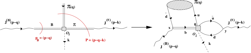
Figure 32: Sum rule calculation of the $B\rightarrow\pi\pi$ decay. The shaded oval region denotes nonperturbative input, the pion distribution amplitude. The other pion and the $B$ meson are represented by the currents $J^{(\pi)}(p-k)$ and $J^{(B)}(p-q)$, respectively. The square represents the four-quark operators $O_{i}$.

Take $p^{2}=k^{2}=q^{2}=0$, and consider the region of large spacelike momenta,

$$|(p-k)^{2}|\sim|(p-q)^{2}|\sim|P^{2}|\gg\Lambda_{\rm QCD}^{2}\,,$$ (163)

in which the correlation function is explicitly calculable by means of OPE. The decomposition of the correlation function in Eq. (160) in the independent momentum structures contains four invariant amplitudes,

$$F_{\nu}^{(O)}=(p-k)_{\nu}F^{(O)}+q_{\nu}\widetilde{F}_{1}^{(O)}+k_{\nu}\widetilde{F}_{2}^{(O)}+\epsilon_{\nu\beta\lambda\rho}q^{\beta}p^{\lambda}k^{\rho}\widetilde{F}_{3}^{(O)}\,,$$ (164)

for the operators $O=O_{1},\widetilde{O}_{1}$, where only the amplitude $F^{(O)}$ is relevant. The procedure to derive a double dispersion relation is as follows [261]. One first makes a dispersion relation in a pion channel of momentum $(p-k)^{2}$ and applies the quark-hadron duality for this channel. Thereafter, to extract the physical $B$ meson state, one performs an analytical continuation of the invariant mass $P^{2}$ to its positive value, $P^{2}=m_{B}^{2}$. This procedure is analogous to the one in the transition from spacelike to timelike form factors. Finally, a dispersion relation in the $B$ meson channel of momentum $(p-q)^{2}$ is derived, together with the application of the quark-hadron duality [20].

At the diagrammatical level, there are four topologically different contributions to the correlation function in Eq. (160), corresponding to four possible combinations of $\bar{u}$ and $d$ fields in the pion distribution amplitude $\langle 0\mid\bar{u}_{\alpha}(z_{1})d_{\beta}(z_{2})\mid\pi^{-}\rangle$, with $z_{1}=0$ or $y$, and $z_{2}=x$ or $y$, $\alpha,\beta$ being the spinor indices. Drawing the quark diagrams, one finds that each contribution yields a $B\to\pi\pi$ matrix element with a certain quark topology: emission ($z_{1}=0$, $z_{2}=x$), annihilation ($z_{1}=0$, $z_{2}=y$), penguin ($z_{1}=y$, $z_{2}=x$) and penguin annihilation ($z_{1}=z_{2}=y$). So far, only the emission topology $F_{\nu E}^{(O)}$ has been calculated [20].

For the matrix elements of $O_{1}$, the factorizable diagrams are those, in which the quarks of the heavy-light currents do not interact with the quarks of the light-quark currents. A typical example is shown in Fig. 33(a). To calculate the factorizable contribution, one inserts an intermediate vacuum state between the weak currents of the operator $O_{1}$. Equation (160) is then converted into a product of two disconnected two-point correlation functions,

$$F^{(O_{1})}_{\nu E}(p,q,k)=\Bigg{(}i\!\int d^{4}y\;e^{i(p-k)\cdot y}\langle\,0\mid T[j^{(\pi)}_{\nu 5}(y)\bar{d}(0)\gamma_{\mu}\gamma_{5}u(0)]\mid 0\rangle\Bigg{)}$$

$$\times\Bigg{(}i\!\int d^{4}x\;e^{i(p-q)\cdot x}\langle\,0\mid T[\bar{u}(0)\gamma^{\mu}b(0)j^{(B)}_{5}(x)]\mid\pi^{-}(q)\rangle\Bigg{)}\,.$$ (165)

The analysis then reduces to that of the $B\to\pi$ transition form factors.

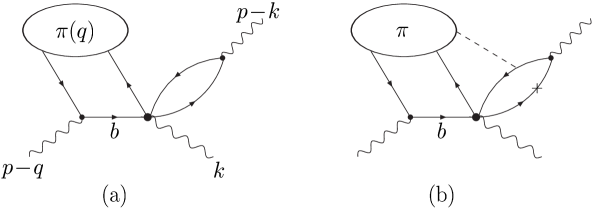
Figure 33: Diagrams corresponding (a) to the leading-order of the correlation function in Eq. (160) for $O=O_{1}$; (b) to the higher-twist soft-gluon nonfactorizable contribution for $O=\widetilde{O}_{1}$. Solid, dashed and wavy lines represent quarks, gluons, and external momenta, respectively. Thick points denote the weak interaction vertices, and ovals the pion distribution amplitudes. The cross represents another attachment of the gluon.

For the operator $O_{1}$, nonfactorizable corrections to Eq. (160), appearing at a two-gluon level, are negligible. In the case of $\widetilde{O}_{1}$, nonfactorizable effects start at the one-gluon level. The relevant correlation function $F_{\nu}^{(\widetilde{O}_{1})}$ receives contributions of hard gluon exchanges, whose $O(\alpha_{s})$ examples are shown in Fig. 34. These two-loop diagrams, not yet calculated because of their complexity, are very important: they give the scale dependence of the matrix element, which partially compensates the scale dependence of the Wilson coefficients $C_{1,2}$ in the effective weak Hamiltonian. Moreover, the analytic continuation of these two-loop contributions in $P^{2}$ generates an imaginary part, which is essential for predicting the CP asymmetries in the $B\to\pi\pi$ decays. The diagrams in Figs. 34(a) and 34(b) correspond to the corrections to the weak decay vertex in the literature. Figure 34(c) corresponds to the hard spectator contribution. However, as explained before, the soft and perturbative contributions in the QCDF, PQCD and LCSR approaches all have different definitions.

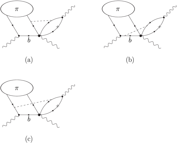
Figure 34: Diagrams corresponding to the $O(\alpha_{s})$ nonfactorizable contributions to the correlation function in Eq. (160) for $O=\widetilde{O}_{1}$.

There is another type of nonfactorizable effects, which comes from the diagram with on-shell gluons being emitted from the quarks of the pion current and absorbed into the pion distribution amplitude, as shown in Fig. 33(b). In terms of the light-cone expansion these contributions are of higher twist, starting from twist 3. It has been argued that the higher-twist nonfactorizable effects are suppressed by a power of $1/m_{B}$ compared to the twist-2 factorizable amplitude [20]. To quantify the magnitude of the nonfactorizable effect from the twist-3 pion distribution amplitude, the ratio has been introduced,

$$\frac{\lambda_{E}(\bar{B}^{0}_{d}\to\pi^{+}\pi^{-})}{m_{B}}\equiv\frac{A^{(\widetilde{O}_{1})}_{E}(\bar{B}^{0}_{d}\to\pi^{+}\pi^{-})}{A^{(O_{1})}_{E}(\bar{B}^{0}_{d}\to\pi^{+}\pi^{-})}\;.$$ (166)

$\lambda_{E}$ was estimated to be

$$\lambda_{E}(\bar{B}^{0}_{d}\to\pi^{+}\pi^{-})=0.05\div 0.15~{}\mbox{GeV}\,,$$ (167)

indicating that nonfactorizable soft corrections from the twsit-3 pion distribution amplitude appeared to be numerically small ($\sim 1\%$).

Recently, a piece of higher-order contribution to the $B\to\pi\pi$ decays from the chromomagnetic dipole operator $O_{8g}$ (gluonic penguin) has been evaluated in LCSR [175]. Similarly, consider the ratio

$$r^{(O_{8g})}(\bar{B}^{0}_{d}\to\pi^{+}\pi^{-})=\frac{A^{(O_{8g})}(\bar{B}^{0}_{d}\to\pi^{+}\pi^{-})}{A^{(O_{1})}_{E}(\bar{B}^{0}_{d}\to\pi^{+}\pi^{-})}\,,$$ (168)

which determines (up to the known Wilson coefficient $C_{8g}$) the gluonic-penguin correction to the factorizable $B\to\pi\pi$ decay amplitude. The result

$$r^{(O_{8g})}(\bar{B}^{0}_{d}\to\pi^{+}\pi^{-})=0.035\pm 0.015\;,$$ (169)

is of the same order of magnitude as $\lambda_{E}$ in Eq. (167). Though the impact of gluonic penguins on the $\bar{B}^{0}_{d}\to\pi^{+}\pi^{-}$ mode is very small, it might be noticeable for the $\bar{B}^{0}_{d}\to\pi^{0}\pi^{0}$ mode [175].

6 Charmed Decays

6.1 Transition Form Factors

$B$ and $D$ meson hadronic matrix elements play a crucial role in the determination of the CKM matrix elements and in overconstraining the unitarity triangle of the Standard Model. The $B\to D^{(*)}$ transitions are defined by the matrix elements,

$$\langle D(P_{2})|{\bar{b}}(0)\gamma_{\mu}c(0)|B(P_{1})\rangle = \sqrt{m_{B}m_{D}}\left[\xi_{+}(\eta)(v_{1}+v_{2})_{\mu}+\xi_{-}(\eta)(v_{1}-v_{2})_{\mu}\right]\;,$$

$$\langle D^{*}(P_{2},\epsilon)|{\bar{b}}(0)\gamma_{\mu}\gamma_{5}c(0)|B(P_{1})\rangle = \sqrt{m_{B}m_{D^{*}}}\left[{\xi_{A1}}(\eta)(\eta+1)\epsilon^{*}_{\mu}-{\xi_{A2}}(\eta)\epsilon^{*}\cdot v_{1}v_{1\mu}\right.$$

$$\left.-{\xi_{A3}}(\eta)\epsilon^{*}\cdot v_{1}v_{2\mu}\right]\;,$$

$$\langle D^{*}(P_{2},\epsilon)|{\bar{b}}(0)\gamma_{\mu}c(0)|B(P_{1})\rangle = i\sqrt{m_{B}m_{D^{*}}}\xi_{V}(\eta)\epsilon^{\mu\nu\alpha\beta}\epsilon^{*}_{\nu}v_{2\alpha}v_{1\beta}\;,$$ (170)

with the velocity transfer $\eta=v_{1}\cdot v_{2}$, $v_{1}=P_{1}/m_{B}$ and $v_{2}=P_{2}/m_{D^{(*)}}$. The form factors $\xi_{+}$, $\xi_{-}$, $\xi_{A_{1}}$, $\xi_{A_{2}}$, $\xi_{A_{3}}$, and $\xi_{V}$ satisfy the relations in the heavy quark limit,

$$\xi_{+}=\xi_{V}=\xi_{A_{1}}=\xi_{A_{3}}=\xi,\;\;\;\;\xi_{-}=\xi_{A_{2}}=0\;,$$ (171)

where $\xi$ is the Isgur-Wise (IW) function [262].

The $O(1/m_{c})$ corrections introduce four new functions [263], and the $O(1/m_{b})$ corrections do not [214]. Taking the matrix elements of the vector current as an example, one has

$$\xi_{+} = \xi\left[1+\left(\frac{1}{m_{c}}+\frac{1}{m_{b}}\right)\rho_{1}\right],$$

$$\xi_{-} = \xi\left(\frac{1}{m_{c}}-\frac{1}{m_{b}}\right)\left(-\frac{\varepsilon}{2}+\rho_{4}\right),$$ (172)

$$\xi_{V} = \xi\left[1+\left(\frac{1}{m_{c}}+\frac{1}{m_{b}}\right)\frac{\varepsilon}{2}+\frac{\rho_{2}}{m_{c}}+\frac{\rho_{1}-\rho_{4}}{m_{b}}\right],$$

with the mass difference $\varepsilon=m_{B}-m_{b}=m_{D}-m_{c}=m_{D^{*}}-m_{c}$, all of which are equal up to $1/m$ corrections. The Luke’s theorem [214, 263, 264] leads to the values of the subleading form factors at zero recoil, $\rho_{1}(1)=0$, $\rho_{2}(1)=0$. It is essential to examine these $1/m$ corrections, especially those from $1/m_{c}$. If they are modest, HQET will be self-consistent and useful.

The form factors in Eq. (170) have been calculated using QCD sum rules at finite $m_{b}$, $m_{c}$ in [265, 266]. HQET sum rules for the IW function were derived in [267, 268], which coincide with the limit $m_{b,c}\to\infty$ of the QCD sum-rule calculation. The above results for finite and infinite masses were compared in [269]. There are two alternative ways to obtain sum rules for the subleading form factors $\rho_{i}$. One can either expand the known finite-mass QCD results to the first order in $1/m$, or start from the HQET Lagrangian and currents in the first power in $1/m$. It has been noticed that the slope of $\xi(\eta)$ near $\eta=1$ depends on how to model the contribution from the continuum state on the hadron side [267, 268, 270].

Figure 35: Isgur-Wise form factor $\xi(\eta)$ for different Borel parameters.

Figure 36: $1/m$ correction form factors $\rho_{1}(\eta)$ (solid curves), $\rho_{2}(\eta)$ (dashed curves), and $\rho_{4}(\eta)$ (dashed-dotted curves) in the unit of 100 MeV.

The sum rule for $\xi(\eta)$ is well known [267, 268], whose results for several Borel parameters are shown in Fig. 35. The predictions for the $1/m$-correction form factors $\rho_{1,2,4}(\eta)$ are presented in Fig. 36 [270]. The curves of $\rho_{1,2}(\eta)$ are pinned at the origin by the Luke’s theorem, and increase for $\eta>1$. $\rho_{4}(\eta)$ is small and nearly constant. Variation of the results with the Borel parameter can be employed to estimate their accuracy. Hence, it is expected that the $O(1/m)$ corrections to the $B\to D^{(*)}$ transition form factors are at most 10%. The above analysis provides the behavior of the $B\to D$ transition form factors with the velocity transfer, but the values at zero recoil, which are specially important for the extraction of the CKM matrix element $|V_{cb}|$, remain intact.

The IW function near the zero recoil is parametrized as

$$\xi(\eta)=F_{B\to D^{(*)}}(1)[1-{\hat{\rho}}^{2}_{D^{(*)}}(\eta-1)+{\hat{c}}_{D^{(*)}}(\eta-1)^{2}+O((\eta-1)^{3})]\;.$$ (173)

Including the $1/m$ and radiative corrections, the normalizations $F_{B\to D}(1)=0.98\pm 0.07$ and $F_{B\to D^{*}}(1)=0.91\pm 0.03$ have been derived in [271]. These normalizations can also be studied in lattice QCD, and the results are

$$F_{B\rightarrow D}(1) = 1.058\pm 0.016\pm 0.003^{+0.014}_{-0.005}\;\;\cite[cite]{[\@@bibref{}{SH1}{}{}]}\;,$$

$$F_{B\rightarrow D^{\ast}}(1) = 0.9130^{+0.0238}_{-0.0173}{}^{+0.0171}_{-0.0302}\;\;\cite[cite]{[\@@bibref{}{SH2}{}{}]}\;.$$ (174)

The errors come from fitting, matching lattice gauge theory and HQET to QCD, lattice spacing dependence, light quark mass dependence and the quenched approximation. The above values agree with those from other methods, such as non-relativistic quark models [274] and a zero-recoil sum rule [275, 276]. For a QCD sum-rule analysis of the subleading form factors involved in the semileptonic decays $B\to D_{1}l\bar{\nu}$ and $B\to D_{2}^{*}l\bar{\nu}$, refer to [277].

The LFQCD formalism has been applied to the $B\to D^{*}$ form factors, whose results can be found in [278].

The PQCD formalism for $B\to D^{(*)}$ transitions has been developed recently [279], which applies under the hierachy,

$$m_{B}\gg m_{D^{(*)}}\gg\Lambda\;,$$ (175)

with $m_{D^{(*)}}$ being the $D^{(*)}$ meson mass. The relation $m_{B}\gg m_{D^{(*)}}$ justifies perturbative evaluation of the $B\to D^{(*)}$ form factors at large recoil and the definition of light-cone $D^{(*)}$ meson wave functions. The relation $m_{D^{(*)}}\gg\Lambda$ justifies the power expansion in the parameter $\Lambda/m_{D^{(*)}}$. Equation (175), corresponding to the heavy quark and large recoil limits, may not be realistic. Nevertheless, an attempt to construct a self-consistent theory under this hierachy is worthwhile.

It has been argued that the wave function for an energetic $D^{(*)}$ meson absorbs collinear dynamics, but with the $c$ quark line being eikonalized. That is, its definition is a mixture of those for a $B$ meson dominated by soft dynamics and for a pion dominated by collinear dynamics. The behavior of the heavy meson wave functions under Eq. (175) has been examined. For $\Lambda/m_{B}$, $\Lambda/m_{D^{(*)}}\ll 1$, only a single $B$ meson wave function $\phi_{+}(x)$ and a single $D^{(*)}$ meson wave function $\phi_{D^{(*)}}(x)$ are involved in the $B\to D^{(*)}$ form factors, $x$ being the momentum fraction associated with the light spectator quark. Equations of motion for the relevant nonlocal matrix elements imply that $\phi_{+}(x)$ and $\phi_{D^{(*)}}(x)$ exhibit maxima at $x\sim\Lambda/m_{B}$ and at $x\sim\Lambda/m_{D^{(*)}}$, respectively. To proceed a numerical analysis, the simple model [279],

$$\phi_{D^{(*)}}(x)=\frac{3}{\sqrt{2N_{c}}}f_{D^{(*)}}x(1-x)[1+C_{D^{(*)}}(1-2x)]\;,$$ (176)

has been adopted. The free shape parameter $C_{D^{(*)}}$ is expected to take a value, such that $\phi_{D^{(*)}}$ has a maximum at $x\sim\Lambda/m_{D^{(*)}}$. The intrinsic $b$ dependence of the $D$ meson wave function was not included.

Figure 37: (a) [(b)] $\xi$ as a function of the velocity transfer from the $B\to D^{(*)}l\nu$ decay. The solid lines represent the central values, the dashed (dot-dashed) lines give the bounds from the linear (quadratic) fits. The circles correspond to $C_{D^{(*)}}=0.5$, 0.7, and 0.9 from bottom to top.

The free parameters $C_{D^{(*)}}$ can be fixed by fitting the leading-power PQCD predictions to the measured decay spectra [280, 281, 282]. With the normalization given in Eq. (174), the linear and quadratic fits to the data give [280, 281]

$${\hat{\rho}}^{2}_{D}=0.69\pm 0.14\;,\;\;\;\;{\hat{c}}_{D}=0\;,\;\;\;\;{\hat{\rho}}^{2}_{D^{*}}=0.81\pm 0.12\;,\;\;\;\;{\hat{c}}_{D^{*}}=0\;,$$

$${\hat{\rho}}^{2}_{D}=0.69^{+0.42}_{-0.15}\;,\;\;\;\;{\hat{c}}_{D}=0.00^{+0.59}_{-0.00}\;,$$ (177)

respectively. Choosing the decay constants $f_{B}=190$ MeV and $f_{D}=f_{D^{*}}=240$ MeV, it has been found that $C_{D}\sim C_{D^{*}}=0.7\pm 0.2$ leads to an excellent agreement with the data as exhibited in Fig. 37. For these values, the corresponding $D^{(*)}$ meson distribution amplitude shows a maximum at $x\sim 0.36$, consistent with the expectation. The rough equality of $C_{D}$ and $C_{D^{*}}$ hints that the heavy quark symmetry holds well. It has been shown that the leading PQCD factorization formulas $B\to D^{(*)}$ transitions indeed respect the heavy quark symmetry.

6.2 $B\to D\pi$

The recent measurement of the $\bar{B}^{0}\to D^{0}\pi^{0}$ branching ratio reveals interesting QCD dynamics. In naive (or generalized) FA, nonfactorizable effects are parameterized through the phenomenological coefficients $a_{i}^{\rm eff}$ in Eq. (145), which depend on the color and Dirac structure of the operators, but otherwise are postulated to be universal [212, 214, 283]. Class-1 and class-2 decay topologies refer to the cases, where a charged and a neutral final-state meson are produced from the four-quark operators, respectively. For instance, the decay $\bar{B}^{0}\to D^{+}\pi^{-}$ is a class-1 process, in which the charged pion is generated at the weak vertex, whereas $\bar{B}^{0}\to D^{0}\pi^{0}$ is a class-2 process, in which the $D^{0}$ meson is directly produced. The corresponding amplitudes are then expressed as

$$A(\bar{B}^{0}\to D^{+}\pi^{-}) = i\,\frac{G_{F}}{\sqrt{2}}\,V_{cb}V_{ud}^{*}\,(m_{B}^{2}-m_{D}^{2})\,f_{\pi}\,F_{0}^{BD}(m_{\pi}^{2})\,a_{1}(D\pi)\,,$$

$$\sqrt{2}\,A(\bar{B}^{0}\to D^{0}\pi^{0}) = i\,\frac{G_{F}}{\sqrt{2}}\,V_{cb}V_{ud}^{*}\,(m_{B}^{2}-m_{\pi}^{2})\,f_{D}\,F_{0}^{B\pi}(m_{D}^{2})\,a_{2}(D\pi)\,,$$ (178)

where the coefficients have the orders of magnitude $a_{1}(D\pi)\sim O(1)$ and $a_{2}(D\pi)\sim O(1/N_{c})$. The isospin symmetry then implies

$$A(B^{-}\to D^{0}\pi^{-})=A(\bar{B}^{0}\to D^{+}\pi^{-})+\sqrt{2}\,A(\bar{B}^{0}\to D^{0}\pi^{0})\,.$$ (179)

Decay mode	Belle [285]	CLEO [286]
$\bar{B}^{0}\to D^{0}\pi^{0}$	$3.1\pm 0.4\pm 0.5$	$2.74^{+0.36}_{-0.32}\pm 0.55$
$\bar{B}^{0}\to D^{*0}\pi^{0}$	$2.7^{+0.8+0.5}_{-0.7-0.6}$	$2.20^{+0.59}_{-0.52}\pm 0.79$
$\bar{B}^{0}\to D^{0}\eta$	$1.4^{+0.5}_{-0.4}\pm 0.3$
$\bar{B}^{0}\to D^{*0}\eta$	$2.0^{+0.9}_{-0.8}\pm 0.4$
$\bar{B}^{0}\to D^{0}\omega$	$1.8\pm 0.5^{+0.4}_{-0.3}$
$\bar{B}^{0}\to D^{*0}\omega$	$3.1^{+1.3}_{-1.1}\pm 0.8$

Table 8: Data (in units of $10^{-4}$) of the $\bar{B}^{0}\to D^{(*)0}M^{0}$ $(M=\pi,\eta,\omega)$ branching ratios.

Within errors, the class-1 decays $\bar{B}^{0}\to D^{(*)+}M^{-}$ with $M=\pi,\rho,a_{1},D_{s},D_{s}^{*}$ can be described using a universal value $|a_{1}|\approx 1.1\pm 0.1$, whereas the class-2 decays $\bar{B}\to\bar{K}^{(*)}M$ with $M=J/\psi,\psi(2S)$ suggest a nearly universal value $|a_{2}|\approx 0.2$–0.3 [284]. The wide range of $|a_{2}|$ is due to the uncertainty in the $B\to K^{(*)}$ form factors. Moreover, the class-3 decays $B^{-}\to D^{(*)0}M^{-}$ with $M=\pi,\rho$, which are sensitive to the interference of the two decay topologies, could be explained by a real, positive ratio $a_{2}/a_{1}\approx 0.2$–0.3, which seemed to agree with the determinations of $|a_{1}|$ and $|a_{2}|$ from other modes. The observed branching ratios of the color-suppressed modes are listed in Table 8 [285, 286]. The parameter $a_{2}$ extracted from Table 8 falls into the range of $|a_{2}(D\pi)|\sim 0.35-0.60$ and $|a_{2}(D^{*}\pi)|\sim 0.25-0.50$ [287]. The phases of $a_{2}/a_{1}$ are $59^{\circ}$ for the $D\pi$ system and $63^{\circ}$ for $D^{*}\pi$ [287], implying sizeable relative strong-interaction phases between class-1 and class-2 $\bar{B}\to D^{(*)}\pi$ decay amplitudes [288, 289]. These results can be regarded as a failure of naive FA: the parameters $a_{2}$ in different types of decays such as $\bar{B}\to D^{(*)}\,\pi$ and $\bar{B}\to\bar{K}^{(*)}J/\psi$ differ by almost a factor 2 in magnitude, indicating a strong nonuniversality of nonfactorizable effects.

If the $c$ quark is treated as a massive quark, QCDF does not apply to the class-2 decays $\bar{B}^{0}\to D^{(*)0}M^{0}$, because of the uncancelled end-point singularities. Therefore, the magnitude and phase of the $a_{2}(D^{(*)}M)$ parameters are not calculable in QCDF. However, these decays are calculable in the PQCD approach based on $k_{T}$ factorization theorem, in which the end-point singularity does not exist. From the power counting rules proposed in Eq. (175) [279], it has been shown that the relative importance of the different topologies of diagrams for the $B\to D\pi$ decays is roughly

$${\rm emission}:{\rm nonfactorizable}\sim 1:\frac{m_{D}}{m_{B}}\;,$$ (180)

which approaches $1:\Lambda/m_{B}$ as the $D$ meson mass $m_{D}$ reduces to the pion mass of $O(\Lambda)$. Since the factorizable and nonfactorizable diagrams contribute to the parameters $a_{1}$ and $a_{2}$ in PQCD, respectively, the ratio $|a_{2}|/a_{1}\sim 0.5$ is obtained. Moreover, the imaginary nonfactorizable amplitudes determine the relative phase of the factorizable and nonfactorizable contributions, which is about $-57^{o}$.

To obtain the above results, the $D^{(*)}$ meson wave function determined from the semileptonic $B\to D^{(*)}l\nu$ decay in the previous subsection has been adopted. Therefore, there is no free parameter in the above calculation. The PQCD predictions for the $B\to D\pi$ branching ratios [290],

$$B(B^{-}\to D^{0}\pi^{-})\sim 5.5\times 10^{-3}\;,$$

$$B({\bar{B}}^{0}\to D^{+}\pi^{-})\sim 2.8\times 10^{-3}\;,$$

$$B({\bar{B}}^{0}\to D^{0}\pi^{0})\sim 2.6\times 10^{-4}\;,$$ (181)

are consistent with the experimental data [285, 286, 291]. The conclusion that the $B\to D^{0}\pi^{0}$ data hint large final-state interaction was drawn from the analyses based on FA [287, 288, 292, 293]. Hence, it is more reasonable to conclude that experimental data just hint large strong phases, but do not tell which mechanism generates these phases [294]. From the viewpoint of PQCD, these strong phases are of short distance, and produced from hard kernels. For the application of the PQCD approach to other charmed nonleptonic decays, refer to [295].

6.3 Decays into Charmonia

The $B$ meson decays into charmonia, such as $B\to J/\psi K$, are theoretically notorious. As defined above, this mode belongs to the color-suppressed class-2 decays, in which one expects large nonfactorizable contributions. Experimentally, the measurement of the branching ratios [296],

$$B(B^{+}\rightarrow J/\psi K^{+}) = (10.1\pm 0.3\pm 0.5)\times 10^{-4}\,,$$

$$B(B^{0}\rightarrow J/\psi K^{0}) = (8.3\pm 0.4\pm 0.5)\times 10^{-4}\,,$$ (182)

provides the information of the coefficient $a_{2}(J/\psi K)$, being of order $0.20-0.30$ [284]. However, it is very difficult to understand such a large $a_{2}(J/\psi K)$, and also those for other similar decays into charmonia: the observed branching ratio differs from the naive FA prediction by at least a factor of 3. In this subsection I discuss the attempts made in the LCSR and QCDF approaches, and explain why they fail.

The QCDF method is usually not applicable, if the emitted meson is heavy. Take the $\bar{B}^{0}\to D^{0}\pi^{0}$ decay as an example. Since the $D^{0}$ meson is not a compact object with small transverse extension, it will strongly interact with the $(B\pi)$ system, such that the factorization breaks down. The parameter $a_{2}(\pi D)$ has been roughly estimated in [69] by treating the charmed meson as a light meson, which is certainly a dubious approximation. Fortunately, QCDF is applicable to the $B\to J/\psi K$ decay, because the transverse size of $J/\psi$ becomes small in the heavy quark limit. However, a recent study [297] indicates that the leading-twist (twist-2) contributions from QCDF are too small to explain the data.

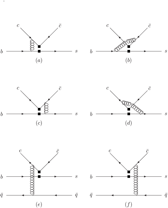
Figure 38: Feynman diagrams for nonfactorizable corrections to $\overline{B}\rightarrow J/\psi K$.

The authors of [298] then calculated twist-3 contributions from the diagrams in Fig. 38. The result for Figs. 38(a)-38(d) is free of the end-point singularity. The contribution from Fig. 38(e) and 38(f) is written, up to twist 3, as

$$f_{II}=f_{II}^{(2)}+f_{II}^{(3)}+\cdots,$$ (183)

where the superscript denotes the twist of the kaon distribution amplitude. The expressions for $f_{II}^{(2)}$ and $f_{II}^{(3)}$ are

$$f^{(2)}_{II} = {4\pi^{2}\over N_{c}}\,{f_{K}f_{B}\over F_{+}^{BK}(m^{2}_{J/\psi})m^{2}_{B}}\,{1\over 1-r}\int^{1}_{0}dx_{1}\,{\phi_{+}(x_{1})\over x_{1}}\int^{1}_{0}dx_{2}\,{\phi_{J/\psi}(x_{2})\over x_{2}}\int^{1}_{0}dx_{3}\,{\phi_{K}(x_{3})\over x_{3}}\;,$$ (184)

$$f^{(3)}_{II} = \left({2m_{0}\over m_{B}}\right)\,{4\pi^{2}\over N_{c}}\,{f_{K}f_{B}\over F_{+}^{BK}(m^{2}_{J/\psi})m_{B}^{2}}\int^{1}_{0}{dx_{1}\over x_{1}}\,\phi_{+}(x_{1})\int^{1}_{0}{dx_{2}\over x_{2}}\,\phi_{J/\psi}(x_{2})\int^{1}_{0}{dx_{3}\over x_{3}^{2}}\,{\phi_{K}^{\sigma}(x_{3})\over 6(1-r)^{3}}\;,$$ (185)

with the mass ratio $r\equiv m_{J/\psi}^{2}/m_{B}^{2}$ and the $B\rightarrow K$ transition form factor $F_{+}^{BK}(m_{J/\psi}^{2})$ being evaluated at the $J/\psi$ meson mass. The twist-2 and one of the two-parton twist-3 distribution amplitudes are given, in their asymptotic form, by

$$\phi_{K}(x)=6x(1-x)\;,\;\;\;\;\phi_{K}^{\sigma}(x)=6x(1-x)\;,$$ (186)

respectively. It is observed that $f^{(2)}_{II}$ is finite, because the potential logarithmic divergence cancels between Fig. 38(e) and 38(f). $f^{3}_{II}$ is singular, since only the potential linear divergence cancels, leaving the logarithmic one.

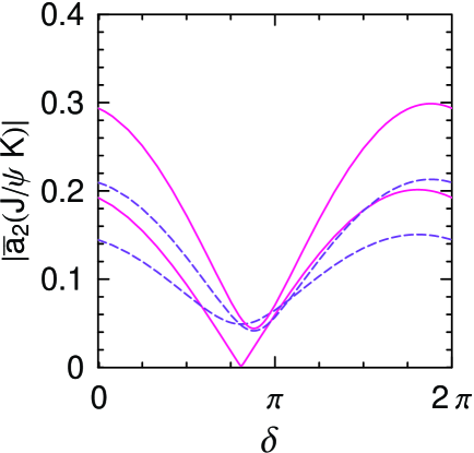
Figure 39: The coefficient $|\bar{a}_{2}(J/\psi K)|$ vs. the phase of the parameter $r$. Solid and dashed curves are for $|\rho|=6$ and 3, respectively. The upper and lower solid curves are for $r=m_{J/\psi}^{2}/m_{b}^{2}$ and $m_{J/\psi}^{2}/m_{B}^{2}$, respectively, and likewise for the dashed curves.

To estimate the twist-3 effect, the divergent integral has been parametrized as [298]

$$X\equiv\int^{1}_{0}{dx_{3}\over x_{3}}=\ln\left({m_{B}\over\Lambda_{\rm QCD}}\right)+\rho,$$ (187)

as in Eq. (149), with $\rho=|\rho|\exp(i\delta)$ being a complex random number. The variation of $|a_{2}(J/\psi K)|$ with the arbitrary parameter $\rho$ is exhibited in Fig. 39 [298], which implies that $|a_{2}(J/\psi K)|$ can fit the data, only when $|\rho|$ is almost as large as 6. For such a huge subleading contribution, the self-consistency of the QCDF analysis is in doubt.

A worse situation has been observed: QCDF breaks down for the $B\to\chi_{c1}K$ deacy even at twist 2 [299]. Similarly, the function $f_{II}$ is obtained by computing the two spectator corrections in Figs. 38(e) and 38(f), whose contribution is given by

$$f_{II}=\frac{4\pi^{2}}{N_{c}}\frac{f_{K}f_{B}}{F_{+}^{BK}(m_{\chi_{c1}}^{2})m_{B}^{2}}\frac{1}{1-r}\int_{0}^{1}dx_{1}\frac{\phi_{+}(x_{1})}{x_{1}}\int_{0}^{1}dx_{3}\frac{\phi_{K}(x_{3})}{x_{3}}\int_{0}^{1}dx_{2}{\phi_{\chi_{c1}}(x_{2})}\left[\frac{1}{x_{2}}+\frac{2r}{x_{3}(1-r)}\right]\;,$$ (188)

with the mass ratio $r=m_{\chi_{c1}}/m_{B}$. Obviously, the integral over $x_{3}$ in Eq. (188) gives logarithmic divergence. Therefore, QCDF breaks down even at leading twist. This is different from the $B\rightarrow J/\psi K$ decay, which does not have logarithmic divergence at leading twist [297, 298]. The reason is that the logarithmic divergences arising from the contribution of the vector and tensor currents are cancelled out in the $B\rightarrow J/\psi K$ decay, while there is no such cancellation for the $B\rightarrow\chi_{c1}K$ decay.

The logarithmically divergent integral has been parametrized in the same way as in Eq. (187). In [299], the parameter $X$ is chosen as $X\approx 2.4$ to make a rough estimate. For $\phi_{\chi_{c1}}(x)=\delta(x-1/2)$, $B(\overline{B}\rightarrow\chi_{c1}K)=0.16\times 10^{-4}$ was obtained [299]. The measured branching ratio [301]

$$B(B^{0}\rightarrow\chi_{c1}K^{0})=(5.4\pm 1.4)\times 10^{-4},$$ (189)

is about thirty times larger than the theoretical prediction. Choosing $X\approx 2.4$, instead of around 6 [298], the QCDF prediction for the $B\to J/\psi K$ branching ratio is also too small.

The end-point singularity becomes more serious in the $B^{+}\rightarrow\chi_{c0}K^{+}$ mode. In the previous calculations, the contribution of the four vertex diagrams in Fig. 38 is infrared safe. However, for the $B\rightarrow\chi_{c0}K$ decay [299], these four diagrams produce infrared divergences. The QCDF predictions for the $B\to\eta_{c}^{(^{\prime})}K$ branching ratios, thought infrared safe, are also too small [300]. The above analyses indicate that it is difficult to apply QCDF to $B$ meson decays into charmonia.

I now turn to the LCSR approach. For the $B\rightarrow J/\psi K$ decay, the relevant operators are

$$O_{1}=(\overline{c}\Gamma_{\mu}c)(\overline{s}\Gamma^{\mu}b)\;,\;\;\;\;\tilde{O}_{1}=\left(\overline{c}\Gamma_{\mu}\frac{\lambda_{a}}{2}c\right)\left(\overline{s}\Gamma^{\mu}\frac{\lambda_{a}}{2}b\right)\;.$$ (190)

In the factorization limit, the matrix element of $\tilde{O}_{1}$ vanishes, and the matrix element of the operator $O_{1}$ can be factorized into

$$\langle J/\psi(p,\epsilon)K(q)|O_{1}|B(p+q)\rangle = \langle J/\psi(p,\epsilon)|\overline{c}\Gamma_{\mu}c|0\rangle\langle K(q)|\overline{s}\Gamma^{\mu}b|B(p+q)\rangle$$ (191)

$$= 2\epsilon\cdot q\,m_{J/\psi}f_{J/\psi}F_{+}^{BK}(m_{J/\psi}^{2})\,,$$

with $f_{J/\psi}$ being the $J/\psi$ meson decay constant. The $B\rightarrow K$ transition form factor $F_{+}^{BK}(m_{J/\psi}^{2})=0.55\pm 0.05$ [261] was obtained using LCSR in a way the same as for the $B\rightarrow\pi$ form factor. Evaluating the $B\rightarrow J/\psi K$ branching ratio with the next-to-leading-order Wilson coefficients, one arrives at [261]

$$B(B\rightarrow J/\psi K)^{fact}=3.3\times 10^{-4}\,.$$ (192)

This value, representing a prediction from FA, is too small compared to the experimental data in Eq. (182).

Similarly, the nonfactorizable contribution associated with the operator ${\tilde{O}}_{1}$ starts at the one-gluon level, and that with $O_{1}$ starts at the two-gluon level. One then considers only the matrix element of ${\tilde{O}}_{1}$, which is expressed as

$$\langle J/\psi K|{\tilde{O}}_{1}(\mu)|B\rangle=2\epsilon\cdot q\,m_{J/\psi}f_{J/\psi}\tilde{F}^{BK}_{+}(\mu^{2})\;.$$ (193)

To calculate the factor $\tilde{F}^{BK}_{+}$, one studies the correlation function,

$$F_{\nu}(p,q,k)=i^{2}\int d^{4}xe^{-i(p+q)\cdot x}\int d^{4}ye^{i(p-k)\cdot y}\langle K(q)|T[J_{\nu}^{(J/\psi)}(y)O(0)J_{5}^{(B)}(x)]|0\rangle\;,$$ (194)

with the interpolating currents $J_{\nu}^{(J/\Psi)}=\overline{c}\gamma_{\nu}c$ and $J_{5}^{(B)}=m_{b}\overline{b}i\gamma_{5}u$, and follows the derivation for the $B\rightarrow\pi\pi$ decays in Sec. 5.4.

The results are $\tilde{F}_{+}^{BK(3)}(\mu_{b})=0.003-0.0055$ from the twist-3 kaon distribution amplitudes and $\tilde{F}_{+}^{BK(4)}(\mu_{b})=0.006-0.0012$ from the twist-4 kaon distribution amplitudes with the scale $\mu_{b}\simeq m_{b}/2$. The wide range for $\tilde{F}_{+}^{BK}$ is attributed to the variation of sum-rule parameters. Combined with the factorizable contribution, one derives the effective parameter $a_{2}$,

$$a_{2}\sim 0.14-0.17\,|_{\mu=\mu_{b}}\,,$$ (195)

which is still too small.

Since the PQCD approach based on $k_{T}$ factorization is free from end-point singularities, it is applicable to $B$ meson decays into charmonia. The formalism for the color-suppressed nonfactorizable amplitude is the same as that for the $\bar{B}\to D^{0}\pi^{0}$ decay in the previous subsection. The $B\to J/\psi K^{(*)}$ decays have been analyzed recently [302, 303], and the predicted branching ratios, together with the experimental data, are listed in Table 9. Briefly speaking, the measured $B^{0}\to J/\Psi K^{0}$ branching ratio [301] is employed to determine the unknown $J/\psi$ meson wave function. This wave function is then used to predict the $B^{0}\to J/\Psi K^{*0}$ branching ratio, whose consistency with the data is obvious.

Mode	Belle [304]	BaBar [301]	PQCD
$J/\Psi K^{0}$	$7.9\pm 0.4\pm 0.9$	$8.3\pm 0.4\pm 0.5$	$8.3$
$J/\Psi K^{*0}$	$12.9\pm 0.5\pm 1.3$	$12.4\pm 0.5\pm 0.9$	$13.37$

Table 9: PQCD results of the $B\to J/\psi K^{(*)}$ branching ratios in unit of $10^{-4}$ with the $J/\psi$ meson decay constant $f_{J/\Psi}=0.405$ GeV.

7 Other Topics

7.1 Final-State Interaction

A strong phase can come from short-distance dynamics and from long-distance dynamics. The former may be calculable, but the latter is completely nonperturbative. The strong phases for two-body nonleptonic $B$ meson decays, derived in the QCDF or PQCD approaches, are all of the short-distance type. That is, the long-distance phases from final-state interaction (FSI) have been neglected in both approaches. It is then essential to look for any means to justify this assumption. In this subsection I review the recent study on this subtle and complicated topic.

Most estimates of FSI effects in the literature [305] suffer ambiguities or difficulties. Some opinions favor small FSI effects in two-body nonleptonic $B$ meson decays. For example, the smallness of FSI effects has been put forward based on the color-transparency argument [67]. The renormalization-group analysis of soft gluon exchanges among initial- and final-state mesons [306] has indicated that FSI effects are not important in two-body $B$ meson decays. For a limited number of decay channels, one can extract the FSI phases $\Delta\delta$ directly from experiments. The phases are large for $D$ meson decays [307] and small for $B$ meson decays [308]:

$$\Delta\delta = 80^{\circ}\pm 7^{\circ};\;\;D\rightarrow K^{-}\pi^{+}/\overline{K}^{0}\pi^{+},$$ (196)

$$\Delta\delta < \left\{\begin{array}[]{ll}11^{\circ};&B\rightarrow D^{+}\pi^{-}/D^{0}\pi^{-}\\ 16^{\circ};&B\rightarrow D^{+}\rho^{-}/D^{0}\rho^{-}\\ 29^{\circ};&B\rightarrow D^{*+}\pi^{-}/D^{*0}\pi^{-}.\\ \end{array}\right.$$ (200)

implying that FSI phases diminish as the initial mass increases [309].

However, an opposite opinion was raised in [309]. Take the decay $B^{+}(\overline{b}u)\rightarrow K^{0}(\overline{s}d)\pi^{+}(\overline{d}u)$ as an example. The gluons exchanged between $\overline{d}$ and $\overline{s}$ (or $d$) are hard, but the gluons between the soft spectator $u$ and $\overline{s}$ (or $d$) are not so hard. By simple kinematics, the invariant mass $m_{\overline{d}u}\approx(\Lambda_{\rm QCD}m_{B})^{1/2}\simeq$ 1.2 GeV for $E_{u}\simeq\Lambda_{\rm QCD}$ is in the middle of the resonance region of the ${\overline{s}d}$ channel. Then long-distance interactions cannot be ignored between $K^{0}$ and $\pi^{+}$.

Some attempts have been made to estimate FSI effects. Applying the time-reversal operation on the decay amplitude $A_{n}=\langle n^{out}|O|B\rangle$, one obtains

$$A_{n}\stackrel{{\scriptstyle T}}{{\rightarrow}}\langle B|TOT^{-1}|n^{in}\rangle\;.$$ (201)

Insert a complete set of out states, and employ the symmetry propery $S_{nn^{\prime}}=S_{n^{\prime}n}$, $S_{nn^{\prime}}=\langle n^{out}|n^{\prime in}\rangle$. From the time reversal invariance of strong interaction, Eq. (201) becomes

$$A_{n}=\sum_{n^{\prime}}S_{nn^{\prime}}A_{n^{\prime}}^{*}\;,$$ (202)

for a T-even decay operator $O$. Subtracting the complex conjugate of $A$ from both sides in Eq.(202) and dividing it by $i$, the familiar relation emerges

$$2{\rm Im}A_{n}=\sum_{n^{\prime}}t_{nn^{\prime}}A_{n^{\prime}}^{*}\;,$$ (203)

with $t=(S-1)/i$. The above expression states that the strong phase is the sum of the contributions over all intermediate states $n^{\prime}$.

If approximating the intermediate states $n^{\prime}$ by two-body states, those connected to the final state $n$ by Pomeron exchange dominate in the sum, and $t_{nn^{\prime}}$ will be almost imaginary. The decay amplitude $A_{n}$ will be also almost imaginary, no matter what operator is responsible for the decay. Certainly, this approximation may not be justified. Without the two-body-state approximation, one can take advantage of the presence of many states. A statistical approach or a random approximation then helps [310]. Note that since $A_{n^{\prime}}$ and $S_{nn^{\prime}}$ come from two different sources, weak and strong interactions, the phase of product $S_{n^{\prime}n}A_{n^{\prime}}^{*}$ for $n^{\prime}\neq n$ takes equally likely a positive or a negative value as $n^{\prime}$ is varied with $n$ fixed. While $A_{n^{\prime}}$ is related to $A_{n}$ ($n^{\prime}\neq n$) by rescattering, there exist so many states that the influence of $n$ on $n^{\prime}$ can be disregarded. Therefore, the phase of $S_{nn^{\prime}}A_{n^{\prime}}^{*}$ takes random values as $n^{\prime}$ varies. Under this approximation, a typical FSI phase in the $B\to\pi\pi$ and $K\pi$ decays has been estimated to be about $20^{o}$ from the meson-meson scattering at 5 GeV [311]. The limitation of the random approximation is that one can only compute the statistically likely values of FSI phases as their standard deviations from zero, instead of predicting values of individual phases.

Figure 40: A model FSI phase.

Figure 41: The enhancement (suppression) factor $E$ vs $E_{max}$. The lower curve ($E<1$) for $\delta(s^{\prime})>0$ shown here, and the upper curve for $\delta(s^{\prime})\rightarrow-\delta(s^{\prime})$.

FSI not only generates a strong phase but also changes a magnitude of amplitude. It has been argued that the decay amplitude could be enhanced by a FSI factor [312],

$$E=\exp\biggl{(}\frac{{\cal P}}{\pi}\int^{\infty}_{s_{\rm th}}\frac{\delta(s^{\prime})}{s^{\prime}-m_{B}^{2}}ds^{\prime}\biggr{)}\;.$$ (204)

In the approximation of two-body intermediate states, the FSI phase approaches $\pm 90^{\circ}$ at high energies. The enhancement or suppression effect is then very large due to a constructive integration over $s^{\prime}$. In the random approximation, the sign of $\delta(s^{\prime})$ may fluctuate with $s^{\prime}$. In this case, the effect of enhancement and suppression would be much smaller. An estimate for the $B\rightarrow K\pi$, $\pi\pi$ decays with one model FSI phase motivated by experiments has been performed. Choose the FSI phase as shown in Fig. 40 [309]: $\delta(s^{\prime})$ rises to large values ($\sim 90^{\circ}$) around 2 GeV and falls linearly to zero at $E_{\rm max}=O(m_{B})$. This $\delta(s^{\prime})$ suppresses the decay amplitude, as indicated by the lower curve in Fig. 41, since the support of the phase integral is mostly below $m_{B}$, where $1/(s^{\prime}-m_{B}^{2})$ is negative. A 10$\sim$40% correction to the decay amplitude is possible [309].

An application of Eq. (202) to the study of the $B\to D\pi$ decays was provided in [293]. The matrix equation can be formally solved to give

$$A=S^{1/2}A^{0}\;,$$ (205)

where $A^{0}$ is an arbitrary real vector of the same dimension as $A$. One may consider the vector $A^{0}$ as representing the decay amplitude in the absence of the final state phases from strong interaction. Assume elastic final state rescattering in the $\bar{B}\to D\pi$ modes. Assigning the real factorization amplitudes in FA to $A^{0}$, one obtains

$$\left(\begin{array}[]{l}A_{D^{0}\pi^{-}}\\ A_{D^{+}\pi^{-}}\\ A_{D^{0}\pi^{0}}\end{array}\right)=S^{1/2}\,\left(\begin{array}[]{l}A^{f}_{D^{0}\pi^{-}}\\ A^{f}_{D^{+}\pi^{-}}\\ A^{f}_{D^{0}\pi^{0}}\end{array}\right)\;,$$ (206)

where the superscript $f$ denotes FA.

Figure 42: Pictorial representation of (a) $r_{e}$ (charge exchange), (b) $r_{a}$ (annihilation) and (c) $r_{0}$ (singlet exchange).

To obtain $S^{1/2}$, one derives the scattering matrix $t$ through the optical theorem. This way makes transparent the mechanism involved in final-state rescattering [293]. By means of Eq. (203) and the various scattering mechanism displayed in Fig. 42, one has

$$t=\left(\begin{array}[]{ccc}r_{0}^{*}+r^{*}_{e}&0&0\\ 0&r^{*}_{0}+r^{*}_{a}&{1\over\sqrt{2}}(r^{*}_{a}-r^{*}_{e})\\ 0&{1\over\sqrt{2}}(r^{*}_{a}-r^{*}_{e})&r^{*}_{0}+{1\over 2}(r^{*}_{a}+r^{*}_{e})\\ \end{array}\right)\;,$$ (207)

where $r_{e}$, $r_{a}$, and $r_{0}$ parametrize the rescattering effects from charge exchange, annihilation, and flavor singlet (Pomeron) exchange, respectively, as defined in Fig. 42. The definition $S=1+it$ then gives the constraints,

$$r_{0}+r_{e} = 2\sin\delta_{3/2}\,e^{i\delta_{3/2}},$$

$$r_{0}+{1\over 2}(3r_{a}-r_{e}) = 2\sin\delta_{1/2}\,e^{i\delta_{1/2}}\;,$$ (208)

where $\delta_{1/2}$ and $\delta_{3/2}$ are the phases associated with the corresponding isospin amplitudes.

To perform the global fit, the data are put into the left-hand side of Eq. (206). The amplitudes in FA with $a_{2}/a_{1}\sim 0.25$ (input from the $B\to J/\psi K$ decay) and some model form factors are put into the right-hand side. The numerical analysis leads to [293]

$$(1+ir_{0})e^{-2i\delta_{3/2}}=0.45+0.50i\;,$$

$$ir_{e}e^{-2i\delta_{3/2}}=0.55-0.50i\;,$$

$$ir_{a}e^{-2i\delta_{3/2}}=0.14+0.04i\;.$$ (209)

One then realizes the relative importance of the various rescattering mechanism: the Pomeron exchange and the charge exchange give roughly similar effect, larger than that from the annihilation mechanism. It was then concluded that FSI is crucial for enhancing $a_{2}$ from 0.25 for the $B\to J/\psi K$ decay to 0.5 for the $\bar{B}^{0}\to D^{0}\pi^{0}$ decay [293]. Similar formalism has been applied to two-body charmless modes, and large FSI phases were also postulated.

I emphasize that the major assumption in the above analysis is the absence of short-distance phases in two-body nonleptonic $B$ meson decays. If short-distance phases exist, the decay amplitudes in Fig. 42 have carried phases already before rescattering. Therefore, the absence of short-distance phases must be assumed, so that the amplitudes before rescattering can be identified as the real amplitudes on the right-hand side of Eq. (206). If short-distance phases do exist, the FSI effects could be small, and the conclusion on the relative importance of different mechanism might be altered. For example, the $B\to D\pi$ branching ratios can be accounted for in the PQCD approach without resort to FSI as shown in Sec. 6.2.

A stringent test of the small FSI assumption is provided by measuring the $B\to KK$ decays. In particular, large observed $B_{d}^{0}\to K^{\pm}K^{\mp}$ branching ratios and CP asymmetry in the $B_{d}^{0}\to K^{0}{\bar{K}}^{0}$ modes will imply large FSI effects. So far, the PQCD predictions for the branching ratios [313],

$$B(B^{+}\to K^{+}K^{0})=1.47\times 10^{-6}\;,$$

$$B(B^{-}\to K^{-}K^{0})=1.84\times 10^{-6}\;,$$

$$B(B_{d}^{0}\to K^{+}K^{-})=3.27\times 10^{-8}\;,$$

$$B({\bar{B}}_{d}^{0}\to K^{-}K^{+})=5.90\times 10^{-8}\;,$$

$$B(B_{d}^{0}\to K^{0}{\bar{K}}^{0})=1.75\times 10^{-6}\;,$$

$$B({\bar{B}}_{d}^{0}\to K^{0}{\bar{K}}^{0})=1.75\times 10^{-6}\;.$$ (210)

are still below the experimental bounds.

7.2 Intrinsic Charm and Charming Penguin

One of the higher-power contributions comes from the Fock states of arbitrarily many particles. For example, a $B$ meson bound state contains

$$|B^{-}\rangle=\psi_{b\bar{u}}|b\bar{u}\rangle+\psi_{b\bar{u}g}|b\bar{u}g\rangle+\psi_{b\bar{u}d\bar{d}}|b\bar{u}d\bar{d}\rangle+\psi_{b\bar{u}c\bar{c}}|b\bar{u}c\bar{c}\rangle+\cdots.$$ (211)

The Fock state decomposition is usually performed at equal light-cone time using light-cone quantization in the gauge $A^{+}=0$ [314, 315]. The non-valence partons in the higher Fock states are generated by QCD splitting mechanism. All the partons in a Fock component are almost on mass shell with long lifetimes, and interact with each other through multiple infrared gluon exchanges. This is the reason they are intrinsic to the hadron structure. The intrinsic heavy quarks are part of the hadron bound state [316]. Due to the hierachical structure of the CKM matrix elements, the weak transition $b\to sc{\overline{c}}$ is doubly Cabibbo enhanced with respect to the $b\to su{\overline{u}}$ transition. This is the argument for the potential importance of the intrinsic charm (IC) [317]. In contrast, a perturbative correction to the weak transition matrix element can produce a $c\bar{c}$ pair through gluon splitting. The quark pair is generally not multiply connected to the partons of the bound state, and extrinsic to the hadron structure. Generally, “intrinsic” contributions in $B$ meson decays are of higher twist, whereas “extrinsic” contributions are of higher order in $\alpha_{s}$.

Some estimates based on phenomenological hints suggest that the IC probability in the $B$ meson could be as large as a few percent [318]. The slight excess in the inclusive $B\to J/\psi X$ yield at low $J/\psi$ momentum [319] implies the presence of the $\bar{B}\to J/\psi D^{(*)}$ channel, which occurs through IC, though such an effect could also be generated by the $\bar{B}\to J/\psi\Lambda\bar{n}$ decay [320]. IC could help to understand the large $B\to\eta^{\prime}K\;,\eta^{\prime}X$ branching ratios. A valence $c\bar{c}$ component in the $\eta^{\prime}$ meson has been introduced to resolve this discrepancy [321], but the decay constant $f_{\eta^{\prime}}^{(c)}\sim-2$ MeV, defined via $\langle 0|{\bar{c}}\gamma_{\mu}\gamma_{5}c|\eta^{\prime}(p)\rangle\equiv if_{\eta^{\prime}}^{(c)}p_{\mu}$, is too small [322]. Discussions on the above subjects can be found in [323]. It was proposed recently [324] that IC in the $B$ meson could be probed by measuring the $B\to J/\psi e\nu X$ decay.

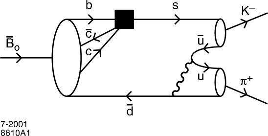
Figure 43: Intrinsic charm in the B-meson can mediate the decay to a strange, charmless final state via the weak transition $b\to sc{\overline{c}}$.

As emphasized in [317], IC plays an important role in the $B\to K\pi$ decays. Considering only the valence contribution, the decay amplitude $A(B^{0}\to K^{+}\pi^{-})$ is written as [325]

$$A(B_{d}^{0}\to K^{+}\pi^{-})=V_{us}V_{ub}^{\ast}(E_{1}-P_{1}^{\rm GIM})-V_{ts}V_{tb}^{\ast}P_{1}\;.$$ (212)

The parameter $E_{1}$ denotes the contribution from the $W$ emission topologies, $P_{1}$ denotes the penguin topologies, and $P_{1}^{\rm GIM}$ contains penguin contributions, which vanish in the $m_{c}=m_{u}$ limit. Beyond the valence approximation, the additional contribution of IC through Fig. 43 arises, which is expressed as $V_{cs}V_{cb}^{\ast}A_{1}^{\rm IC}$. There are no hard gluon exchanges across the weak vertex in Fig. 43, so that the computation of the hard scattering amplitude factorizes. One portion of the weak vertex mediates the annihilation of the ${\bar{b}}c$ quarks, and the other describes the amplitude for the $(c\bar{q})$ state to emerge with the parton content of the $K\pi$ final state, namely ${\bar{s}}q^{\prime}q{\bar{q}}$. Note that the above two pieces of the hard scattering kernels are in fact convoluted together over the momentum fraction of the light-cone wave function for the $(b\bar{c})(c\bar{q})$ state, which is still unknown.

The amplitude for the $(c\bar{q})$ state to emerge as ${\bar{s}}q^{\prime}q{\bar{q}}$ cosmetically resembles Fig. 28(f). Hence, the IC contribution has been parametrized as [317]

$$A_{1}^{\rm IC}(s,q,B,K,\pi)\sim f_{B_{c}^{\ast}}F_{a}^{P}\frac{a_{1}(m_{b}/2)}{a_{6}(m_{b}/2)}B\;,$$ (213)

where $f_{B_{c}^{\ast}}\sim 0.317$ GeV [326] arises from the annihilation of the $\bar{b}c$ pair, and the remaining factors come from an estimate of the lower half of the diagram in Fig. 43. The factorizable annihilation amplitude $F_{a}^{P}$ has been calculated in the PQCD approach [25]. It is easy to get ${a_{1}(m_{b}/2)}/{a_{6}(m_{b}/2)}\sim-20$. The parameter $B$ reflects the probability amplitude to find the B meson in an IC configuration, as well as an adjustment for the $\sim$ 50% penguin enhancement [25]. Hence, one has $B\sim 2(0.02)/3$. The impact of IC on the $B\to K\pi$ decays has been investigated in [317] based on Eq. (213), and the results are exhibited in Fig. 44. Note that IC can act to either enhance or decrease the CP asymmetry. The IC contribution $|A_{1}^{\rm IC}|/|P_{1}|\sim O(10)\%$ is a nontrivial fraction of the penguin parameter $P_{1}$, which reflects the accuracy we can reach in calculating the effective value of $P_{1}$.

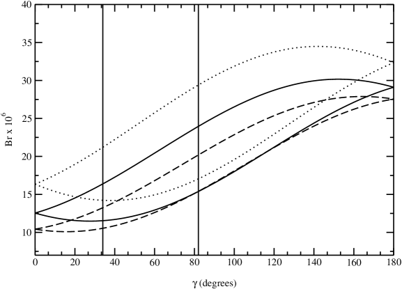
Figure 44: Intrinsic charm in the B-meson can mediate the decay to a strange, charmless final state via the weak transition $b\to sc{\overline{c}}$.

“Charming penguins” refer to the nonperturbative piece of the extrinsic $c$ quark loop, whose contributions are parametrized into a term $\tilde{P}_{1}$. Theoretically, their importance is not clear. However, a recent analysis of the $B\to K\pi$, $\pi\pi$, $K\eta$, and $K\eta^{\prime}$ decays indicates that they could be important. The parameter $\tilde{P}_{1}$ includes not only the charming penguin contributions, but also annihilation and penguin contractions of penguin operators. It does not include leading emission amplitudes of penguin operators ($O_{3}$–$O_{6}$), which have been explicitly evaluated in FA. In this respect, it is a general parameterization of all the perturbative and nonperturbative $O(\Lambda_{\rm QCD}/m_{b})$ contributions of the operators $O_{5}$ and $O_{6}$. $\tilde{P}_{1}$ has the same quantum numbers and physical effects as the original charming penguins proposed in [328].

The charming penguin contribution in $\tilde{P}_{1}$ can be, taking the $B_{d}^{0}\to K^{+}\pi^{-}$ decay as an example, included in the term $P_{1}$ in Eq. (212). Another $O(\Lambda_{\rm QCD}/m_{b})$ contribution from the GIM-penguin $\tilde{P}_{1}^{GIM}$ has been neglected for simplicity [228]. The $B\to K\pi$ data do not constrain this parameter very effectively, since its contribution is doubly Cabibbo suppressed with respect to $\tilde{P}_{1}$. The remaining $\pi^{+}\pi^{-}$ mode alone is not sufficient to fully determine the complex parameter $\tilde{P}_{1}^{GIM}$. However, the GIM-penguin contribution may be able to enhance the ${\cal B}(B\to\pi^{0}\pi^{0})$ up to few $\times 10^{-6}$ [329].

$|V_{cb}|\!\times\!10^{3}$	$|V_{ub}|\!\times\!10^{3}$	$\hat{B}_{K}$	$f_{B_{d}}\sqrt{B_{d}}$ (MeV)	$\xi$
$40.9\!\pm\!1.0$	$3.70\!\pm\!0.42$	$0.86\!\pm\!0.06\!\pm\!0.14$	$230\!\pm\!30\!\pm\!15$	$1.16\!\pm\!0.03\!\pm\!0.04$
$F_{K}(M_{K}^{2})$	$B(K^{+}\pi^{-})\!\times\!10^{6}$	$B(K^{+}\pi^{0})\!\times\!10^{6}$	$B(K^{0}\pi^{+})\!\times\!10^{6}$	$B(K^{0}\pi^{0})\!\times\!10^{6}$
$0.32\pm 0.12$	$18.6\pm 1.1$	$11.5\pm 1.3$	$17.9\pm 1.7$	$8.9\pm 2.3$
$F_{\pi}(m_{\pi}^{2})$	$B(\pi^{+}\pi^{-})\!\times\!10^{6}$	$B(\pi^{+}\pi^{0})\!\times\!10^{6}$	$B(\pi^{0}\pi^{0})\!\times\!10^{6}$
$0.27\pm 0.08$	$5.2\pm 0.6$	$4.9\pm 1.1$	$<\!3.4\,$ BaBar

Table 10: Values of the input parameters used in the global fit.

Mode	UTA		$|V_{ub}/V_{cb}|$
	$B$ ($10^{-6}$)	$|A_{CP}|$	$B$ ($10^{-6}$)	$|A_{CP}|$
$\pi^{+}\pi^{-}$	$8.9\pm 3.3$	$0.37\pm 0.17$	$8.7\pm 3.6$	$0.39\pm 0.20$
$\pi^{+}\pi^{0}$	$5.4\pm 2.1$	–	$5.5\pm 2.2$	–
$\pi^{0}\pi^{0}$	$0.44\pm 0.13$	$0.61\pm 0.26$	$0.69\pm 0.27$	$0.45\pm 0.27$
$K^{+}\pi^{-}$	$18.4\pm 1.0$	$0.21\pm 0.10$	$18.8\pm 1.0$	$0.21\pm 0.12$
$K^{+}\pi^{0}$	$10.3\pm 0.9$	$0.22\pm 0.11$	$10.7\pm 1.0$	$0.22\pm 0.13$
$K^{0}\pi^{+}$	$19.3\pm 1.2$	$0.00\pm 0.00$	$18.1\pm 1.5$	$0.00\pm 0.00$
$K^{0}\pi^{0}$	$8.7\pm 0.8$	$0.04\pm 0.02$	$8.2\pm 1.2$	$0.04\pm 0.03$

Table 11: Predictions for CP-averaged branching ratios and absolute values of the CP asymmetries $|A_{CP}|$. The left (right) columns show results obtained using constraints on the CKM parameters $\rho$ and $\eta$ obtained from the unitarity triangle analysis (UTA) [36] (the measurement of $|V_{ub}/V_{cb}|$). The last four channels are those used for fitting the charming penguin parameter $\tilde{P}_{1}$.

Using the inputs collected in Table 10 [228], the complex parameter $\tilde{P}_{1}=(0.13\pm 0.02)\,e^{\pm i(114\pm 35)^{o}}$ in units of $f_{\pi}F^{B\pi}(m_{\pi}^{2})$ has been determined from the data fitting, which has the expected size of $O(\Lambda_{\rm QCD}/m_{b})$. Note that the sign of the phase is practically not constrained by the data. Table 11 [228] shows the predicted CP-averaged branching ratios and the absolute value of the CP-asymmetries $|A_{CP}|$ for the $B\to K\pi$ and $\pi\pi$ modes. The angle $\phi_{3}$ is determined through the effect of interefence terms in the $B\to K\pi$ branching ratios. The nonperturbative parameter $\tilde{P}_{1}$ with an additional phase in the amplitudes makes the extraction of $\phi_{3}$ difficult. It has been checked using the $|V_{ub}/V_{cb}|$-constrained fit that almost any value of $\phi_{3}$ is allowed, given the uncertainty on $\tilde{P}_{1}$.

I stress that the intrinsic penguins and charming penguins represent distinct dynamics. However, both contributions are Cabibbo-enhanced and contain an $O(1)$ Wilson coefficient. Indeed, the parameter $A_{1}^{\rm IC}$ can also be absorbed into $P_{1}$ and $P_{1}^{\rm GIM}$. Hence, a global fit can not distinguish them. Note that the intrinsic penguin contribution in [317] was parametrized to be proportional to the annihilation penguin amplitude calculated in the PQCD approach, such that its phase, including the sign, can be fixed.

8 Conclusion

In this article I have reviewed the two fundamental tools in QCD perturbation theory, collinear and $k_{T}$ factorization theorems, in which soft dynamics and hard dynamics of a process are factorized into hadron wave functions and hard kernels, respectively. Both factorization theorems can be constructed in a gauge-invariant way up to all orders, such that infrared-finite and gauge-invariant predictions are obtained. $k_{T}$ factorization is more appropriate, when the end-point region of parton momentum fractions becomes important. To improve perturbative expansion, threshold resummation for collinear factorization and $k_{T}$ resummation for $k_{T}$ factorization can be performed.

I then discussed the various QCD approaches to exclusive $B$ meson decays available in the literature, which were developed based on the above fundamental concepts for perturbaton theory. I reviewed the recent progress made in these approaches, emphasizing the basic ideas behind and the comparison of their phenomenological implications. The competition among different approaches and the confrontation between theoretical predictions and experimental data have stimulated tremendous progress. In this section I briefly summarize the advantage of each method and the important issues, whcih require further investigation in order for a more solid and complete framework.

The advantage of LCSR is that both soft and hard contributions can be analyzed in the same framework, and that it is easy to examine the self-consistency of expansions in $\alpha_{s}$ and in $1/m_{b}$. Recently, an essential step toward the evaluation of nonfactorizable contributions (from twist-3 hadron distribution amplitudes) has been made. However, the analysis is not yet complete. The urgent subject is to include the nonfactorizable contributions associated with the twist-2 distribution amplitudes, i.e., from the diagrams in Fig. 34. These diagrams can not only moderate the scale dependence of predictions, but introduce strong phases, which are necessary for generating direct CP asymmetries. Since the strong phases come from higher-order contributions, compared to the leading soft transition form factors, they are expected to be small, the same as those from the QCDF approach.

For QCDF, the advantage is its explicit factorization picture in the heavy quark limit. Talking about the treatment of leading contribtuions, it is most complete among all approaches, since the scale and scheme dependences have been greatly reduced. However, the end-point singularity appearing at subleading level (twist-3 nonfactorizable amplitudes and annihilation amplitudes) makes QCDF less predictive. This is also the reason the experimental constraint on the unitarity angles derived from QCDF is not very strong. Except for the end-point singularity, another challenge comes from the explanation of the possible large direct CP asymmetries in the two-body nonleptonic $B$ meson decays.

The PQCD approach, based on $k_{T}$ factorization theorem, is free of the end-point singularities. Therefore, the nonperturbative inputs are only universal hadron distribution amplitudes, without the transition form factors and the arbitrary infrared cutoffs due to the singularities. So far, the PQCD predictions are in agreement with data, and phenomenologically successful. However, it is still under debate whether the crucial Sudakov effect is strong enough to suppress the end-point contribution for the physcial mass $m_{B}\sim 5$ GeV. The urgent subject is then to calculate higher-order corrections, and examine whether they converge. Before proving this, PQCD is not yet a self-consistent theory. The calculation can also verify the argument about the characteristic hard scale $\sqrt{\Lambda m_{B}}$ for exclusive $B$ meson decays, which was made based on the hard-scattering picture. This characteristic scale is the key for PQCD to explain the $B\to VP$ data.

SCET provides the most systematic framework for constructing collinear factorization formulas of exclusive $B$ meson decays at large recoil. Its advantage is that contributions characterized by different scales can be separated easily. A progress has been made recently in deriving the symmetry relations among various transition form factors, and the power corrections and radiative corrections to these relations. However, to make explicit predictions, which can be compared with data, it is necessary to calculate the Wilson coefficients of effective operators from the matching of the effective theory to the full one. The calculation is as complicated as in other approaches.

The advantage of LFQCD is its simplicity. At leading power, the formula for a transition form factor involves only an overlap integral of the initial- and final-state hadron wave fuctions. Both soft dynamics and hard dynamics have been absorbed into the wave functions. The inclusion of nonvalence contributions has been worked out, which is crucial for guaranteeing the covariance of predictions. The next step is to extend the LFQCD to two-body nonleptonic decays, especially to nonfactorizable amplitudes. This extention will be a challenge.

Though some study has been done, the behavior of the $B$ meson bound state is still not clear. This subject is important, since the $B$ meson wave functions, including those associated with higher Fock states (such as intrinsic charms), are the input of all QCD approaches. There is still no reliable method to analyze long-distance FSI effects in exclusive $B$ meson decays. Even an ansatz does not exist, in which the importance of FSI can be determined from data fitting. The ansatz based on the factorization assumption, i.e., on the absence of short-distance phases, is not convincing as explained in Sec. 6.2 and in Sec. 7.1. Another crucial contribution from charming penguins also requires investigation. More clever ideas are necessary for understanding the above nonperturbative dynamics.

As demonstrated in this article, exclusive $B$ meson decays exhibit exciting QCD dynamics, which could be, fortunately, studied in a self-consistent way due to the large $b$ quark mass. Some plausible mechanism has been explored. For example, annihilation contribution may not be as small as we thought with the hint from the possible large CP asymmetry in the $B_{d}^{0}\to\pi^{+}\pi^{-}$ decay. However, more challenging topics are waiting for our effort.

I thank Profs. S. Brodsky and A.I. Sanda for their encouragement and useful discussions. I also thank my collaborators and competitors for their constructive opinions. This work was supported by the National Science Council of R.O.C. under the Grant No. NSC-91-2112-M-001-053.

References

- [1] Y. Nir, hep-ph/0208080.
- [2] M. Kobayashi and T. Maskawa, Prog. Th. Phys. 49 (1973) 652.
- [3] I.I. Bigi and A.I. Sanda, Nucl. Phys. B 193 (1981) 85 .
- [4] M. Gronau and D. London, Phys. Rev. Lett. 65 (1990) 3381 .
- [5] M. Gronau, J.L. Rosner, and D. London, Phys. Rev. Lett. 73 (1994) 21 ; R. Fleischer, Phys. Lett. B 365 (1996) 399 .
- [6] R. Fleischer and T. Mannel, Phys. Rev. D 57 (1998) 2752 .
- [7] M. Neubert and J. Rosner, Phys. Lett. B 441 (1998) 403 ; Phys. Rev. Lett. 81 (1998) 5076 ; M. Neubert, JHEP 9902 (1999) 014.
- [8] A.J. Buras and R. Fleischer, Eur. Phys. J. C 11 (1999) 93 .
- [9] M. Gronau and J.L. Rosner, Phys. Rev. D 65 (2002) 093012 ; Z. Xiao, C.D. Lü, and L. Guo hep-ph/0303070.
- [10] M. Gronau and J.L. Rosner, Phys. Rev. D 66 (2002) 053003 .
- [11] R. Fleischer, Phys. Lett. B 459 (1999) 306 .
- [12] M. Gronau and D. Wyler, Phys. Lett. B 265 (1991) 172 ; M. Gronau, hep-ph/0211282.
- [13] Y. Grossman, Z. Ligeti, and A. Soffer, hep-ph/0210433; D. Atwood and A. Soni, hep-ph/0212071; R. Fleischer, hep-ph/0301256.
- [14] D. Atwood, I. Dunietz and A. Soni, Phys. Rev. Lett. 78 (1997) 3257 ; Phys. Rev. D 63 (2001) 036005 .
- [15] I. Dunietz, Phys. Lett. B 270 (1991) 75 .
- [16] R. Fleischer and D. Wyler, Phys. Rev. D 62 (2000) 057503 .
- [17] Z. Ligeti, hep-ph/0302031.
- [18] V.L. Chernyak and I.R. Zhitnitsky, Nucl. Phys. B 345 (1990) 137 .
- [19] A. Ali, V.M. Braun, and H. Simma, Z. Phys. C 63 (1994) 437 .
- [20] A. Khodjamirian, Nucl. Phys. B 605 (2001) 558 .
- [21] C.Y. Cheung, W.M. Zhang, and G.L. Lin, Phys. Rev. D 52 (1995) 2915 ; W.M. Zhang, G.L. Lin, and C.Y. Cheung, Int. J. Mod. Phys. A 11 (1996) 3297 .
- [22] H.M. Choi and C.R. Ji, Phys. Lett. B 460 (1999) 461 .
- [23] M. Beneke, G. Buchalla, M. Neubert and C.T. Sachrajda, Phys. Rev. Lett. 83 (1999) 1914 .
- [24] H-n. Li and H.L. Yu, Phys. Rev. Lett. 74 (1995) 4388 ; Phys. Lett. B 353 (1995) 301 ; Phys. Rev. D 53 (1996) 2480 .
- [25] Y.Y. Keum, H-n. Li, and A.I. Sanda, Phys. Lett. B 504 (2001) 6 ; Phys. Rev. D 63 (2001) 054008 ; Y.Y. Keum and H-n. Li, Phys. Rev. D 63 (2001) 074006 .
- [26] C.D. Lü, K. Ukai, and M.Z. Yang, Phys. Rev. D 63 (2001) 074009 .
- [27] C.W. Bauer, S. Fleming, and M. Luke, Phys. Rev. D 63 (2001) 014006 .
- [28] C.W. Bauer, S. Fleming, D. Pirjol, and I.W. Stewart, Phys. Rev. D 63 (2001) 114020 .
- [29] R. Fleischer, hep-ph/0210323.
- [30] A.J. Buras, F. Parodi, and A, Stocchi, hep-ph/0207101; A.J. Buras, hep-ph/0210291.
- [31] M. Paulini, hep-ph/0302023.
- [32] X.G. He, C.S. Huang, and X.Q. Li, hep-ph/0210435.
- [33] Y.L. Wu and Y.F. Zhou, hep-ph/0210367.
- [34] Z.Z. Xing, hep-ph/0301024.
- [35] A. Höcker, H. Lacker, S. Laplace and F. Le Diberder, Eur. Phys. J. C 21 (2001) 225 .
- [36] M. Ciuchini et al., JHEP 0107 (2001) 013; M. Ciuchini, Nucl. Phys. Proc. Suppl. 109 (2002) 307 .
- [37] I.P. Gouz et al., hep-ph/0211432.
- [38] M. Diehl and G. Hiller, JHEP 0106 (2001) 067; C.S. Kim, J.P. Lee, and S. Oh, hep-ph/0205262; Phys. Rev. D 67 (2003) 014002 .
- [39] H.Y. Cheng and K.C. Yang, Phys. Rev. D 66 (2002) 014020 ; C.K. Chua, W.S. Hou, and S.Y. Tsai, Phys. Rev. D 66 (2002) 054004 .
- [40] C.H. Chen and H-n. Li, hep-ph/0209043.
- [41] J. Ellis, hep-ph/0211322.
- [42] S. Khalil, hep-ph/0212050.
- [43] S.J. Brodsky and G.P. Lepage, Phys. Lett. B 87 (1979) 359 ; Phys. Rev. Lett. 43 (1979) 545 ; G.P. Lepage and S. Brodsky, Phys. Rev. D 22 (1980) 2157 .
- [44] S.J. Brodsky, Y. Frishman and G.P. Lepage, and C. Sachrajda, Phys. Lett. B 91 (1980) 239 .
- [45] A.V. Efremov and A.V. Radyushkin, Theor. Math. Phys. 42 (1980) 97; Phys. Lett. B 94 (1980) 245 ; I.V. Musatov and A.V. Radyushkin, Phys. Rev. D 56 (1997) 2713 .
- [46] A. Duncan and A.H. Mueller, Phys. Lett. B 90 (1980) 159 ; Phys. Rev. D 21 (1980) 1636 .
- [47] V.L. Chernyak, A.R. Zhitnitsky, and V.G. Serbo, JETP Lett. 26 (1977) 594.
- [48] V.L. Chernyak and A.R. Zhitnitsky, Sov. J. Nucl. Phys. 31 (1980) 544; Phys. Rep. 112 (1984) 173.
- [49] W. Zimmermann, in Elementary Particles in Quantum Field Theory (MIT Press, Cambridge, Mass., 1971).
- [50] H-n. Li, Phys. Rev. D 64 (2001) 014019 ; M. Nagashima and H-n. Li, hep-ph/0202127.
- [51] F. Del Aguila and M.K. Chase, Nucl. Phys. B 193 (1981) 517 .
- [52] E. Braaten, Phys. Rev. D 28 (1983) 524 .
- [53] E.P. Kadantseva, S.V. Mikhailov, Radyushkin, Sov. J. Nucl. Phys. 44 (1986) 326.
- [54] C. Becchi, A. Rouet, and R. Stora, Phys. Lett. B 52 (1974) 344 .
- [55] C.W. Bauer and I.W. Stewart, Phys. Lett. B 516 (2001) 134 .
- [56] C.W. Bauer, D. Pirjol and I.W. Stewart, Phys. Rev. D 65 (2002) 054022 .
- [57] J. Chay and C. Kim, Phys. Rev. D 65 (2002) 114016 ; hep-ph/0205117.
- [58] C.W. Bauer, D. Pirjol, and I.W. Stewart, hep-ph/0205289.
- [59] M. Beneke, A.P. Chapovsky, M. Diehl and T. Feldmann, Nucl. Phys. B 643 (2002) 431 .
- [60] I.W. Stewart, hep-ph/0207253; hep-ph/0209159.
- [61] E. Eichten and B. Hill, Phys. Lett. B 234 (1990) 511 ; B. Grinstein, Nucl. Phys. B 339 (1990) 253 ; H. Georgi, Phys. Lett. B 240 (1990) 447 .
- [62] A.V. Manohar, T. Mehen, D. Pirjol and I.W. Stewart, hep-ph/0204229.
- [63] D. Pirjol and I.W. Stewart, hep-ph/0211251.
- [64] M. Beneke and Th. Feldmann, Phys. Lett. B 553 (2003) 267 .
- [65] C.W. Bauer, S. Fleming, D. Pirjol, I.Z. Rothstein and I.W. Stewart, hep-ph/0202088.
- [66] C.W. Bauer, D. Pirjol and I.W. Stewart, Phys. Rev. Lett. 87 (2001) 201806 ; C.W. Bauer, B. Grinstein, D. Pirjol and I.W. Stewart, hep-ph/0208034.
- [67] J.D. Bjorken, Nucl. Phys. Proc. Suppl. 11 (1989) 325.
- [68] D. Politzer and M. Wise, Phys. Lett. B 257 (1991) 399 .
- [69] M. Beneke, G. Buchalla, M. Neubert and C.T. Sachrajda, Nucl. Phys. B 591 (2000) 313 .
- [70] A. Szczepaniak, E.M. Henley, and S.J. Brodsky, Phys. Lett. B 243 (1990) 287 .
- [71] G. Burdman and J.F. Donoghue, Phys. Lett. B 270 (1991) 55 .
- [72] M. Beneke and T. Feldmann, Nucl. Phys. B 592 (2000) 3 .
- [73] R. Ahkoury, G. Sterman, and Y.P. Yao, Phys. Rev. D 50 (1994) 358 .
- [74] G.P. Korchemsky, D. Pirjol, and T.M. Yan, Phys. Rev. D 61 (2000) 114510 .
- [75] H-n. Li, Phys. Rev. D 66 (2002) 094010 .
- [76] S. Descotes-Genon and C.T. Sachrajda, hep-ph/0209216.
- [77] E. Lunghi, D. Pirjol, and D. Wyler, NPB 649 (2003) 349 .
- [78] S.W. Bosch, R.J. Hill, B.O. Lange, and M. Neubert, hep-ph/0301123.
- [79] E. Gardi et. al., hep-ph/0203161.
- [80] E. Laenen, G. Sterman, and W. Vogelsang, Phys. Rev. Lett. 84 (2000) 4296 ; Phys. Rev. D 63 (2001) 114018 .
- [81] G. Sterman, Phys. Lett. B 179 (1986) 281 ; Nucl. Phys. B 281 (1987) 310 .
- [82] S. Catani and L. Trentadue, Nucl. Phys. B 327 (1989) 323 ; ibid 353 (1991) 183.
- [83] H-n. Li, Phys. Rev. D 55 (1997) 105 .
- [84] H-n. Li, Phys. Lett. B 454 (1999) 328 ; Chin. J. Phys. 37 (1999) 569.
- [85] J. Kwiecinski and B. Ziaja, Phys. Rev. D 60 (1999) 054004 .
- [86] H.L. Lai and H-n. Li, Phys. Lett. B 471 (1999) 220 .
- [87] G.P. Korchemsky and A.V. Radyushkin, Nucl. Phys. B 283 (1987) 342 .
- [88] C.W. Bauer, D. Pirjol, and I.W. Stewart, hep-ph/0211069.
- [89] G. Sterman, An Introduction to Quantum Field Theory, Cambridge, 1993.
- [90] S. Catani, M. Ciafaloni and F. Hautmann, Phys. Lett. B 242 (1990) 97 ; Nucl. Phys. B 366 (1991) 135 .
- [91] J.C. Collins and R.K. Ellis, Nucl. Phys. B 360 (1991) 3 .
- [92] E.M. Levin, M.G. Ryskin, Yu.M. Shabelskii, and A.G. Shuvaev, Sov. J. Nucl. Phys. 53 (1991) 657.
- [93] M.K. Jones et al., Phys. Rev. Lett. 84 (2000) 1398 ; O. Gayou et al., Phys. Rev. Lett. 88 (2002) 092301 .
- [94] J.P. Ralston and P. Jain, hep-ph/0302043.
- [95] J. Botts and G. Sterman, Nucl. Phys. B 225 (1989) 62 .
- [96] H-n. Li and G. Sterman, Nucl. Phys. B 381 (1992) 129 .
- [97] P. Jain et al., Nucl. Phys. A 666 (2000) 75 ; H-n. Li, Nucl. Phys. A 684 (2001) 304 and references therein.
- [98] T. Kurimoto, H-n. Li, and A.I. Sanda, Phys. Rev. D 65 (2002) 014007 .
- [99] Z.T. Wei and M.Z. Yang, Nucl. Phys. B 642 (2002) 263 .
- [100] I.V. Musatov and A.V. Radyushkin, Phys. Rev. D 56 (1997) 2713 .
- [101] J.C. Collins and D.E. Soper, Nucl. Phys. B 194 (1982) 445 .
- [102] M. Nagashima and H-n. Li, hep-ph/0210173.
- [103] A.G. Grozin and M. Neubert, Phys. Rev. D 55 (1997) 272 .
- [104] S. Descotes-Genon and C.T. Sachrajda, Nucl. Phys. B 625 (2002) 239 .
- [105] H. Kawamura, J. Kodaira, C.F. Qiao, and K. Tanaka, Phys. Lett. B 523 (2001) 111 ; Erratum-ibid. 536 (2002) 344.
- [106] V.M. Braun and I.E. Filyanov, Z. Phys. C 48 (1990) 239 ; P. Ball, JHEP 9901 (1999) 010.
- [107] P. Ball, V.M. Braun, Y. Koike and K. Tanaka, Nucl. Phys. B 529 (1998) 323 .
- [108] H. Kawamura, J. Kodaira, C.F. Qiao, and K. Tanaka, hep-ph/0112174.
- [109] B.O. Lange and M. Neubert, hep-ph/0303082.
- [110] M. Bauer and M. Wirbel, Z. Phys. C 42 (1989) 671 .
- [111] C.D. Lu and M.Z. Yang, hep-ph/0212373.
- [112] J.C. Collins and D.E. Soper, Nucl. Phys. B 193 (1981) 381 .
- [113] H-n. Li, Phys. Lett. B 405 (1997) 347 ; hep-ph/9703328; H-n. Li and J.L. Lim, Eur. Phys. J. C 10 (1999) 319 .
- [114] R. Jakob and P. Kroll, Phys. Lett. B 315 (1993) 463 .
- [115] H-n. Li, hep-ph/9803202.
- [116] F. Schlumpf, Phys. Rev. D 50 (1994) 6895 .
- [117] J.C. Collins, in Perturbative Quantum Chromodynamics, ed. A.H. Mueller (World Scientific, Singapore, 1989).
- [118] M.A. Shifman, A.I. Vainshtein, and V.I. Zakharov, Nucl. Phys. B 147 (1979) 385 ; ibid. 147 (1979) 448.
- [119] B.L. Ioffe and A.V. Smilga, Phys. Lett. B 114 (1982) 353 ; Nucl. Phys. B 216 (1983) 373 ; V.A. Nesterenko and A.V. Radyushkin, Phys. Lett. B 115 (410) 82 .
- [120] V.A. Novikov, L.B. Okun, M.A. Shifman, A.I. Vainshtein, M.B. Voloshin, and V.I. Zakharov, Phys. Rep. 41 (1978) 1.
- [121] L.J. Reinders, H. Rubinstein, and S. Yazaki, Phys. Rep. 127 (1985) 1.
- [122] D.J. Broadhurst, Phys. Lett. B 101 (1981) 423 ; T.M. Aliev and V.L. Eletsky, Sov. J. Nucl. Phys. 38 (1983) 936.
- [123] C. Coriano, A. Radyushkin, and G. Sterman, Nucl. Phys. B 405 (1993) 481 .
- [124] A. Khodjamirian and R. Rückl, in Heavy Flavors, 2nd edition, eds., A.J. Buras and M. Lindner (World Scientific, Singapore, 1998), hep-ph/9801443.
- [125] I.I. Balitsky, V.M. Braun, and A.V. Kolesnichenko, Nucl. Phys. B 312 (1989) 509 ; V.M. Braun and I.E. Filyanov, Z. Phys. C 44 (1989) 157 .
- [126] A. Khodjamirian, R. Rückl, S. Weinzierl, and O. Yakovlev, Phys. Lett. B 410 (1997) 275 .
- [127] E. Bagan, P. Ball and V.M. Braun, Phys. Lett. B 417 (1998) 154 .
- [128] V.M. Belyaev, A. Khodjamirian and R. Rückl, Z. Phys. C 60 (1993) 349 .
- [129] V.M. Belyaev, V.M. Braun, A. Khodjamirian and R. Rückl, Phys. Rev. D 51 (1995) 6177 .
- [130] P. Ball, JHEP 9809 (1998) 005; Z. Phys. C 29 (1985) 637 .
- [131] P. Ball and R. Zwicky JHEP 0110 (2001) 019.
- [132] P. Colangelo and A. Khodjamirian, in Boris Ioffe Festschrift At the Frontier of Particle Physics / Handbook of QCD, ed. M. Shifman (World Scientific, Singapore, 2001), hep-ph/0010175.
- [133] A. Khodjamirian, R. Rückl, S. Weinzierl, C.W. Winhart and O. Yakovlev, Phys. Rev. D 62 (2000) 114002 .
- [134] J.M. Flynn, in Proc. of 28th ICHEP, ed. Z. Ajduk and A.K. Wroblewski (World Scientific, Singapore, 1996), hep-lat/9611016.
- [135] UKQCD Colla., K.C. Bowler et al., hep-lat/9910011.
- [136] APE Colla., A. Abada et al., Nucl. Phys. Proc. Suppl. 83 (2000) 268 .
- [137] JLQCD Colla., S. Hashimoto et al., Phys. Rev. D 58 (1998) 014502 .
- [138] Z.G. Wang, M.Z. Zhou, and T. Huang, hep-ph/0212336.
- [139] K.G. Chetyrkin and M. Steinhauser, Eur. Phys. J. C 21 (2001) 319 .
- [140] P. Ball and V.M. Braun, Phys. Rev. D 58 (1998) 094016 ; A. Ali, P. Ball, L.T. Handoko, and G. Hiller, Phys. Rev. D 61 (2000) 074024 .
- [141] A. Khodjamirian, G. Stoll and D. Wyler, Phys. Lett. B 358 (1995) 129 ;
- [142] A. Ali and V.M. Braun, Phys. Lett. B 359 (1995) 223 .
- [143] T.M. Aliev and Savci, hep-ph/0302187.
- [144] D. Becirevic, hep-ph/0211340.
- [145] L. Lellouch, hep-ph/0211359.
- [146] A. El-Khadra et al., Phys. Rev. D 55 (1997) 3933 .
- [147] Z. Sroczynski et al., Nucl. Phys. Proc. Suppl. 83 (2000) 971 .
- [148] S. Ryan, hep-lat/0111010.
- [149] A. El-Khadra et al., Phys. Rev. D 58 (1998) 014506 .
- [150] JLQCD Colla., S. Aoki et al., Nucl. Phys. Proc. Suppl. 63 (1998) 356 .
- [151] MILC Colla., C. Bernard et al., Phys. Rev. Lett. 81 (1998) 4812 .
- [152] CP-PACS Colla., A. Ali Khan et al., Phys. Rev. D 64 (2001) 034505 .
- [153] MILC Colla., S. Datta et al., Nucl. Phys. Proc. Suppl. 94 (2001) 346 .
- [154] A. Ali Khan et al., Phys. Lett. B 427 (1998) 132 .
- [155] JLQCD Colla., K-I. Ishikawa et al., Phys. Rev. D 61 (2000) 074501 .
- [156] CP-PACS Colla., A. Ali Khan et al., Phys. Rev. D 64 (2001) 054504 .
- [157] APE Colla., D. Becirevic et al., Phys. Rev. D 60 (1999) 074501 .
- [158] UKQCD Colla., K. Bowler et al., hep-lat/0007020.
- [159] UKQCD Colla., L. Lellouch and C.J.D. Lin Phys. Rev. D 64 (2001) 094501 .
- [160] C. Davies et al., hep-lat/0110003.
- [161] S. Collins et al., Phys. Rev. D 60 (1999) 074504 .
- [162] MILC Colla., C. Bernard et al., Nucl. Phys. Proc. Suppl. 106 (2002) 412 .
- [163] JLQCD Colla., N. Yamada et al., Nucl. Phys. Proc. Suppl. 106 (2002) 397 .
- [164] S. Sharpe and Y. Zhang, Phys. Rev. D 53 (1996) 5125 .
- [165] UKQCD Colla., K.C. Bowler et al., Phys. Lett. B 486 (2000) 111 .
- [166] APE Colla., A. Abada et al., Nucl. Phys. B 619 (2001) 565 .
- [167] A.X. El-Khadra et al., Phys. Rev. D 64 (2001) 014502 .
- [168] JLQCD Colla., S. Aoki et al., Phys. Rev. D 64 (2001) 114505 .
- [169] J. Shigemitsu et al., hep-lat/0208062.
- [170] D. Becirevic, S. Prelovsek, and J. Zupan, hep-lat/0210048.
- [171] P. Colangelo et al., Phys. Rev. D 53 (3672) 1996 .
- [172] M. Dahm, R. Jakob, and P. Kroll, Z. Phys. C 68 (1995) 595 .
- [173] A. Khodjamirian and R. Rückl, Phys. Rev. D 58 (1998) 054013 .
- [174] A.P. Szczepaniak and A.V. Radyushkin, Phys. Rev. D 59 (1999) 034017 .
- [175] A. Khodjamirian, T. Mannel, and P. Urban, hep-ph/0210378.
- [176] K.C. Bowler et al., Phys. Lett. B 486 (2000) 111 .
- [177] D. Becirevic, Nucl. Phys. Proc. Suppl. 94 (2001) 337.
- [178] P. Ball and V.M. Braun, Phys. Rev. D 58 (1998) 094016 .
- [179] J. Charles, A. Le Yaouanc, L. Oliver, O. Pene, and J.C. Raynal, Phys. Rev. D 60 (1999) 014001 .
- [180] H-n. Li and G.L. Lin, Phys. Rev. D 60 (1999) 054001 .
- [181] M. Dugan and B. Grinstein, Phys. Lett. B 255 (1991) 583 .
- [182] R.J. Hill and M. Neubert, hep-ph/0211018.
- [183] P. Ball and E. Kou, hep-ph/0301135.
- [184] A. Ali and A. Salim Safir, Eur. Phys. J. C 25 (2002) 583 .
- [185] M. Beneke, T. Feldmann, and D. Seidel, Nucl. Phys. B 612 (2001) 25 .
- [186] S.W. Bosch and G. Buchalla, Nucl. Phys. B 621 (2002) 459 ; A. Ali and A.Y. Parkhomenko, Eur. Phys. J. C 23 (2002) 89 .
- [187] C. Greub, T. Hurth and D. Wyler, Phys. Rev. D 54 (1996) 3350 ; A.J. Buras, A. Czarnecki, M. Misiak, and J. Urban, Nucl. Phys. B 631 (2002) 219 .
- [188] S.W. Bosch and G. Buchalla, hep-ph/0208202.
- [189] CLEO Colla., S. Chen et al., Phys. Rev. Lett. 87 (2001) 251807 ; ALEPH Colla., R. Barate et al., Phys. Lett. B 429 (1998) 169 ; Belle Colla., K. Abe et al., Phys. Lett. B 511 (2001) 151 ; Particle Data Group, D.E. Groom et al., Eur. Phys. J. C 15 (2000) 1 ; BABAR Colla., B. Aubert et al., Phys. Rev. Lett. 87 (2001) 241803 .
- [190] M.A. Ivanov and V.E. Lyubovitskij, hep-ph/0211077.
- [191] M.V. Terent’ev, Sov. J. Phys. 24 (1976) 106; V.B. Berestetsky and M.V. Terent’ev, ibid. 24 (1976) 547; ibid. 25 (1977) 347.
- [192] P.L. Chung, F. Coester, and W.N. Polyzou, Phys. Lett. B 205 (1988) 545 .
- [193] W. M. Zhang, Chin. J. Phys. 31 (1994) 717; hep-ph/9510428.
- [194] W. Jaus, Phys. Rev. D 41 (1990) 3394 ; Phys. Rev. D 44 (1991) 2851 ; Z. Phys. C 54 (1992) 611 .
- [195] P.J. O’Donnell and Q.P. Xu, Phys. Lett. B 325 (1994) 219 ; Phys. Lett. B 336 (1994) 113 .
- [196] H.M. Choi, C.R. Ji, and L.S. Kisslinger, Phys. Rev. D 65 (2002) 074032 .
- [197] C.Q. Geng, C.W. Hwang, C.C. Lih, and W.M. Zhang, Phys. Rev. D 64 (2001) 114024 .
- [198] W. Jaus, Phys. Rev. D 53 (1996) 1349 .
- [199] D. Melikhov, Phys. Rev. D 53 (1996) 2460 ; Phys. Lett. B 380 (1996) 363 .
- [200] N.B. Demchuk et al., Phys. Atom. Nucl. 59 (1996) 2152; Yad. Fiz. 59N12 (1996) 2235.
- [201] C.Y. Cheung, C.W. Hwang, and W.M. Zhang, Z. Phys. C 75 (1997) 657 .
- [202] A.Yu. Dubin and A. Kaidalov, Phys. Atom. Nucl. 56 (1993) 237; Yad. Fiz. 56 (1993) 164.
- [203] M. Sawicki, Phys. Rev. D 44 (1991) 433 .
- [204] W. Jaus, Phys. Rev. D 60 (1999) 054026 .
- [205] C.W. Hwang, Phys. Lett. B 530 (2002) 93 .
- [206] C.R. Ji and H.M. Choi, Phys. Lett. B 513 (2001) 330 .
- [207] H.J. Melosh, Phys. Rev. D 9 (1974) 1095 .
- [208] H.Y. Cheng, C.Y. Cheung, and C.W. Hwang, Phys. Rev. D 55 (1997) 1559 .
- [209] C.W. Hwang, Phys. Rev. D 64 (2001) 034011 .
- [210] UKQCD Colla., D.R. Burford et al., Nucl. Phys. B 447 (1995) 425 .
- [211] H.M. Choi and C.R. Ji, Phys. Rev. D 59 (1999) 034001 ; Phys. Lett. B 460 (1999) 461 .
- [212] M. Bauer, B. Stech, M. Wirbel, Z. Phys. C 29 (1985) 637 ; ibid. 34 (1987) 103.
- [213] A.J. Buras and J.M. Gérard, Nucl. Phys. B 264 (1986) 371 ; A.J. Buras, J.M. Gérard, and R. Rückl, Nucl. Phys. B 268 (1986) 16 .
- [214] M. Neubert, V. Rieckert, B. Stech and Q.P. Xu, in Heavy Flavours, ed. A.J. Buras and M. Lindner (World Scientific, Singapore, 1992); M. Neubert and B. Stech, in Heavy Flavours II, ed. A.J. Buras and M. Lindner (World Scientific, Singapore, 1998), hep-ph/9705292.
- [215] M. Bander, D. Silverman, and A. Soni, Phys. Rev. Lett. 43 (1979) 242 .
- [216] H.Y. Cheng, Phys. Lett. B 335 (1994) 428 .
- [217] H.Y. Cheng, Z. Phys. C 69 (1996) 647 .
- [218] J. Soares, Phys. Rev. D 51 (1995) 3518 ; A.N. Kamal and A.B. Santra, Z. Phys. C 72 (1996) 91 ; A.N. Kamal, A.B. Santra, and R.C. Verma, Phys. Rev. D 53 (1996) 2506 .
- [219] A. Ali and C. Greub, Phys. Rev. D 57 (1998) 2996 ; A. Ali, G. Kramer, and C.D. Lu, Phys. Rev. D 59 (1999) 014005 .
- [220] H.Y. Cheng and B. Tseng, Phys. Rev. D 58 (1998) 094005 .
- [221] A.J. Buras and L. Silvestrini, hep-ph/9806278.
- [222] G. Altarelli, G. Curci, G. Martinelli, and S. Petrarca, Nucl. Phys. B 187 (1981) 461 .
- [223] M. Beneke, G. Buchalla, M. Neubert and C.T. Sachrajda, Nucl. Phys. B 606 (2001) 245 .
- [224] J. Chay and C. Kim, hep-ph/0301055; hep-ph/0301262.
- [225] D.S. Du et al., Phys. Rev. D 65 (2002) 074001 ; Phys. Rev. D 65 (2002) 094025 .
- [226] N.G. Deshpande, X.G. He, W.S. Hou and, S. Pakvasa, Phys. Rev. Lett. 82 (1999) 2240 ; W.S. Hou, J.G. Smith, and F. Würthwein, hep-ex/9910014.
- [227] M. Beneke, hep-ph/0207228.
- [228] M. Ciuchini et al., hep-ph/0208048.
- [229] E. Won, hep-ex/0206066; Belle Colla., K. Abe et al., hep-ex/0301032.
- [230] BaBar Colla., B. Aubert et al., hep-ex/0207055.
- [231] G. Buchalla, hep-ph/0302145.
- [232] X.G. He, J.P. Ma, and C.Y. Wu, Phys. Rev. D 63 (2001) 094004 .
- [233] H.Y. Cheng and K.C. Yang, Phys. Rev. D 64 (2001) 074004 .
- [234] D.S. Du et al., Phys. Rev. D 67 (2003) 014023 .
- [235] R. Aleksan et al., hep-ph/0301165.
- [236] X.H. Guo, O. Leitner, and A.W. Thomas, Phys. Rev. D 63 (2001) 056012 .
- [237] M. Beneke and M. Neubert, hep-ph/0210085.
- [238] A. Ali, J. Chay, C. Greub, and P. Ko, Phys. Lett. B 424 (1998) 161 .
- [239] T. Feldmann, P. Kroll, and B. Stech, Phys. Rev. D 58 (1998) 114006 .
- [240] C.H. Chang and H-n. Li, Phys. Rev. D 55 (1997) 5577 .
- [241] T.W. Yeh and H-n. Li, Phys. Rev. D 56 (1997) 1615 .
- [242] H.Y. Cheng, H-n. Li, and K.C. Yang, Phys. Rev. D 60 (1999) 094005 .
- [243] H-n. Li, hep-ph/0110365.
- [244] C.Y. Wu, T.W. Yeh, and H-n. Li, Phys. Rev. D 53 (1996) 4982 ; ibid. 55 (1997) 237.
- [245] H-n. Li and K. Ukai, hep-ph/0211272.
- [246] C.H. Chen, Y.Y. Keum, and H-n. Li, Phys. Rev. D 64 (2001) 112002 ; Phys. Rev. D 66 (2002) 054013 .
- [247] Y.Y. Keum, H-n. Li, and A.I. Sanda, hep-ph/0201103; Y.Y. Keum, hep-ph/0209002; hep-ph/0209208; Y.Y. Keum and A.I. Sanda, hep-ph/0209014.
- [248] J. Rosner, hep-ph/0208243; H. Quinn, talk presented at the 5th KEK International Topic Conference on Frontiers of Flavor Pysics, KEK, Japan, Nov. 2001.
- [249] Y.Y. Keum and H-n. Li, Phys. Rev. D 63 (2001) 074006 .
- [250] C.D. Lü and M.Z. Yang, Eur. Phys. J. C 23 (2002) 275 .
- [251] K. Ukai and A.I. Sanda, Prog. Theor. Phys. 107 (2002) 421 .
- [252] C.H. Chen and H-n. Li, Phys. Rev. D 63 (2001) 014003 .
- [253] C.H. Chen, Phys. Lett. B 525 (2002) 56 .
- [254] R. Bartoldus, talk presented at the First Workshop on Flavor Physics and CP Violation (FPCP), Philadelphia, May, 2002.
- [255] H-n. Li, hep-ph/0103305; hep-ph/0110365.
- [256] S. Mishima, Phys. Lett. B 521 (2002) 252 .
- [257] B. Melic, Phys. Rev. D 59 (1999) 074005 .
- [258] E. Kou and A.I. Sanda, Phys. Lett. B 525 (2002) 240 .
- [259] A. Ali and A.Y. Parkhomenko, Phys. Rev. D 65 (2002) 074020 .
- [260] L. Li, X. Wu, and T. Huang, hep-ph/0212277.
- [261] B. Melic, hep-ph/0209265.
- [262] N. Isgur and M.B. Wise, Phys. Lett. B 232 (1989) 113 ; ibid. 232 (1989) 113.
- [263] M.E. Luke, Phys. Lett. B 252 (1990) 447 .
- [264] C.G. Boyd and D.E. Brahm, Phys. Lett. B 257 (1991) 393 ; R.F. Lebed and M. Suzuki, Phys. Rev. D 44 (1991) 829 ; J.G. Körner and G. Thompson, Phys. Lett. B 264 (1991) 185 .
- [265] V.N. Baier and A.G. Grozin, in Proc. of 9th Int. Conf. on High Energy Physics Problems, JINR, Dubna (1988); Z. Phys. C 47 (1990) 669 .
- [266] A.A. Ovchinnikov and V.A. Slobodenyuk, Z. Phys. C 44 (1989) 433 .
- [267] A.V. Radyushkin, Phys. Lett. B 271 (1991) 218 .
- [268] M. Neubert, Phys. Rev. D 45 (1992) 2451 .
- [269] P. Ball, Phys. Lett. B 281 (1992) 133 .
- [270] V.N. Baier and A.G. Grozin, hep-ph/9908365.
- [271] I. Caprini, L. Lellouch, and M. Neubert, Nucl. Phys. B 530 (1998) 153 .
- [272] S. Hashimoto et al., Nucl. Phys. Proc. Suppl. 73 (1999) 399; Phys. Rev. D 61 (2000) 014502 .
- [273] S. Hashimoto et al., Phys. Rev. D 66 (2002) 014503 ; J.N. Simone et al., Nucl. Phys. Proc. Suppl. 83 (2000) 334; A.S. Kronfeld et al., hep-ph/0207122; hep-ph/0209231.
- [274] A. Falk and M. Neubert, Phys. Rev. D 47 (1993) 2965 ; M. Neubert, Phys. Lett. B 338 (1994) 84 .
- [275] I. Bigi, M. Shifman, and N. Uraltsev, Annu. Rev. Nucl. Part. Sci. 47 (1997) 591.
- [276] M. Shifman, N. Uraltsev and A. Vainstein, Phys. Rev. D 51 (1995) 2217 .
- [277] M.Q. Huang, C.Z. Li, and Y.B. Dai, Phys. Rev. D 61 (2000) 054010 ; M.Q. Huang and Y.B. Dai, Phys. Rev. D 64 (2001) 014034 .
- [278] B.L. G. Bakker, H.M. Choi, and C.R. Ji, hep-ph/0303002.
- [279] T. Kurimoto, H-n. Li, and A.I. Sanda, hep-ph/0210289.
- [280] BELLE Colla., K. Abe et al., Phys. Lett. B 526 (2002) 258 .
- [281] BELLE Colla., K. Abe et al., Phys. Lett. B 526 (2002) 247 .
- [282] CLEO Colla., R.A. Briere et al., Phys. Rev. Lett. 89 (2002) 081803 .
- [283] A. Deandrea, N. Di Bartolomeo, R. Gatto, and G. Nardulli, Phys. Lett. B 318 (1993) 549 .
- [284] H.Y. Cheng and K.C. Yang, Phys. Rev. D 59 (1999) 092004 .
- [285] Belle Colla., K. Abe et al., Phys. Rev. Lett. 88 (2002) 052002 .
- [286] CLEO Colla., T.E. Coan et al., Phys. Rev. Lett. 88 (2002) 062001 .
- [287] H.Y. Cheng, Phys. Rev. D 65 (2002) 094012 .
- [288] M. Neubert and A.A. Petrov, Phys. Lett. B 519 (2001) 50 .
- [289] C.W. Chiang and J.L. Rosner, hep-ph/0212274.
- [290] Y.Y. Keum, T. Kurimoto, H-n. Li, C.D. Lu, and A.I. Sanda, in preparation.
- [291] BaBar Colla., B. Aubert et al., hep-ex/0207092.
- [292] Z.Z. Xing, hep-ph/0107257.
- [293] C.K. Chua, W.S Hou, and K.C. Yang, Phys. Rev. D 65 (2002) 096007 ; hep-ph/0210002.
- [294] J.P. Lee, hep-ph/0109101.
- [295] C.D. Lü, Eur. Phys. J. C 24 (2002) 121 ; C.D. Lü and K. Ukai, hep-ph/0210206.
- [296] BaBar Colla., B. Aubert et al., Phys. Rev. D 65 (2002) 032001 .
- [297] J. Chay and C. Kim, hep-ph/0009244.
- [298] H.Y. Cheng and K.C. Yang, Phys. Rev. D 63 (2001) 074011 .
- [299] Z. Song, C. Meng, and K.T. Chao, hep-ph/0206253.
- [300] Z. Song, C. Meng, and K.T. Chao, hep-ph/0209257.
- [301] BaBar Colla., B. Aubert et al., Phys. Rev. D 65 (2002) 032001 .
- [302] A.I. Sanda, N. Sinha, R. Sinha, and K. Ukai, in Proceedings for the 4th International Workshop on Physics and CP Violation, ed. T. Ohshima and A.I. Sanda (World Scientific, Singapore, 2001).
- [303] C.H. Chen, hep-ph/0302059.
- [304] Belle Collaboration, K. Abe et al., Phys. Lett. B 538 (2002) 11 ; hep-ex/0211047.
- [305] R. Fleischer, Eur. Phys. J. C 6 (1999) 451 ; Phys. Lett. B 435 (1998) 221 ; M. Neubert, Phys. Lett. B 424 (1998) 152 ; H. Jin, hep-ph/9805235; D.S. Du, X.Q. Li, Z.T. Wei and B.S. Zou, Eur. Phys. J. A 4 (1999) 91 ; A.F. Falk, A.L. Kagan, Y. Nir, and A.A. Petrov, Phys. Rev. D 57 (1998) 4290 ; D. Atwood and A. Soni, Phys. Rev. D 58 (1998) 036005 .
- [306] H-n. Li and B. Tseng, Phys. Rev. D 57 (1998) 443 .
- [307] M. Bishai et al., Phys. Rev. Lett. 78 (1997) 3261 .
- [308] M. Suzuki, Phys. Rev. D 58 (1998) 111504 .
- [309] M. Suzuki, hep-ph/0001170.
- [310] R.N. Cahn and M. Suzuki, hep-ph/9708208.
- [311] M. Suzuki and L. Wolfenstein, Phys. Rev. D 60 (1999) 074019 .
- [312] M. Jacob, G. Mahoux, and R. Omnès, Nuovo Cim. 23 (1962) 838.
- [313] C.H. Chen and H-n. Li, Phys. Rev. D 63 (2001) 014003 .
- [314] P.A.M. Dirac, Rev. Mod. Phys. 21 (1949) 392.
- [315] S.J. Brodsky and G.P. Lepage, in Perturbative Quantum Chromodynamics, ed. A.H. Mueller (World Scientific, Singapore, 1989) and references therein.
- [316] S.J. Brodsky, P. Hoyer, C. Peterson, and N. Sakai, Phys. Lett. B 93 (1980) 451 ; S.J. Brodsky, C. Peterson, and N. Sakai, Phys. Rev. D 23 (1981) 2745 .
- [317] S.J. Brodsky and S. Gardner, Phys. Rev. D 65 (2002) 054016 .
- [318] C.H.V. Chang and W.S. Hou, Phys. Rev. D 64 (2001) 071501 .
- [319] CLEO Colla., R. Balest et al., Phys. Rev. D 52 (1995) 2661 .
- [320] S.J. Brodsky and F.S. Navarra, Phys. Lett. B 411 (1997) 152 .
- [321] I. Halperin and A. Zhitnitsky, Phys. Rev. D 56 (1997) 7247 ; Phys. Rev. Lett. 80 (1998) 438 .
- [322] M. Franz, M.V. Polyakov, and K. Goeke, Phys. Rev. D 62 (2000) 074024 .
- [323] S. Gardner, hep-ph/0209080.
- [324] F. Gabbiani, J. Qiu, and G. Valencia, hep-ph/0201159.
- [325] A.J. Buras and L. Silvestrini, Nucl. Phys. B 569 (2000) 3 .
- [326] P. Colangelo, G. Nardulli, and N. Paver, Z. Phys. C 57 (1993) 43 .
- [327] C. Isola, M. Ladisa, G. Nardulli, T.N. Pham, and P. Santorelli, Phys. Rev. D 64 (2001) 014029 ; Phys. Rev. D 65 (2002) 094005 .
- [328] M. Ciuchini, E. Franco, G. Martinelli, and L. Silvestrini, Nucl. Phys. B 501 (1997) 271 ; M. Ciuchini, R. Contino, E. Franco, G. Martinelli, and L. Silvestrini, Nucl. Phys. B 512 (1998) 3 ; Erratum-ibid. 531 (1998) 656.
- [329] M. Ciuchini, E. Franco, G. Martinelli, M. Pierini and L. Silvestrini, Phys. Lett. B 515 (2001) 33 .