Abstract

We review the description of high energy diffraction from both the $s$ and $t$ channel viewpoints, and demonstrate their consistency. We emphasize the role played by $s$ channel unitarity and multi-Pomeron exchanges. We explain how these effects suppress hard diffractive processes. As examples, we describe the calculation of diffractive dijet production at the Tevatron and predict some of the rich diffractive phenomena accessible in proton–nuclear collisions at RHIC.

1 Introduction

A broad class of processes at high energies has properties analogous to the classical pattern of the diffraction of light. These are usually called diffractive processes. The classic example is the elastic scattering of hadrons on nuclei, which has an angular distribution with a series of minima and maxima, analogous to the diffraction of light on a black disc. In diffractive processes the wave nature of particles is clearly revealed and the necessity of a quantum mechanical description in terms of amplitudes, and not probabilities, is evident.

Unitarity relates the imaginary parts of forward elastic scattering amplitudes to total cross sections. Hence studies of elastic scattering and $\sigma_{\rm tot}$ for different targets and projectiles was traditionally one of important source of information on the strengths of interactions and their radii. In particular, data on the high-energy interactions of hadrons indicate that the radius of the strong interaction increases with energy, and indicate that the total cross sections will continue to increase in the energy region not explored at present accelerators.

Processes of diffractive dissociation of colliding particles [1] provide new possibilities for the investigation of the dynamics of high-energy hadronic interactions. These processes are dominated by soft, nonpertubative aspects of QCD, and hence provide important information on the dynamics. Indeed, they provide a rich testing ground for models of soft interactions. In this paper we demonstrate that the cross sections of inelastic diffractive processes are very sensitive to nonlinear, unitarity effects.

A new class of diffractive phenomena—hard diffraction—has been extensively studied both experimentally and theoretically in recent years. These processes include the total cross section and diffractive dissociation of a virtual photon at high energy at HERA, and the diffractive production of jets, $W,Z$ bosons, heavy quarks, etc. in hadronic collisions. The latter processes become possible at very high (c.m.) energies ($\sqrt{s}$) because large mass $M$ diffractive states may be produced with $M^{2}\ll s$. Investigation of these processes gives new possibilities for the study of the interplay of soft and hard dynamics in QCD. An important question—the breaking of QCD factorization for hard reactions in diffractive processes—will be discussed below.

Nowadays diffractive hard processes are attracting attention as a way of extending the physics programme at proton colliders, including novel ways of searching for New Physics, see, for example, [2]–[6] and references therein. An especially interesting process is the exclusive double diffractive production of a Higgs boson at the LHC; $pp\rightarrow p+H+p$, where the $+$ signs denote the presence of large rapidity gaps. Clearly a careful treatment of both the soft and hard QCD effects is crucial for the reliability of the theoretical predictions for these diffractive processes.

The outline of the article is as follows. In Section 2 we review diffraction phenomena from both the $s$ and $t$ channel viewpoints. In Section 2.3 we link these approaches together. We emphasize the convenience of working in terms of diffractive eigenstates, as originally proposed by Good and Walker [7]. In Section 3 we discuss how these eigenstates may be identified with the different parton configurations of the proton. Scattering through each of the eigenstates is suppressed (by unitarity or multi-Pomeron effects) by different amounts. In Section 4 we study some examples of hard diffractive processes. First we summarize a calculation of diffractive dijet production at the Tevatron, which shows that the estimate of the overall suppression of the cross section is in agreement with the data. In Section 4.2 we turn to diffractive proton–nuclear processes. We present predictions for a range of hard diffractive processes which are accessible at RHIC. Finally, Section 5 contains some brief conclusions.

Since this article is an attempt at a short review of high energy diffractive phenomena, we have only provided a few references to help the reader. Hence our reference list is incomplete and we apologize to those authors whose work has not been cited. Section 4 contains new results for diffractive proton–nuclear processes.

2 Theoretical approaches to diffraction at high energies

The investigation of the diffractive scattering of hadrons gives important information on the structure of hadrons and on their interaction mechanisms. Diffractive processes may be studied from either an $s$ channel or $t$ channel viewpoint. We will discuss these approaches in turn, and then show that they are complementary to, and consistent with, each other.

2.1 Diffraction from an $s$ channel viewpoint

Unitarity plays a pivotal role in diffractive processes. The total cross section is intimately related to the elastic scattering amplitude and the scattering into inelastic final states via $s$ channel unitarity, $SS^{\dagger}=I$, or

$${\rm disc}\ T\equiv T-T^{\dagger}=iT^{\dagger}T$$ (1)

with $S=I+iT$. If we were to focus, for example, on elastic unitarity, then disc would simply denote the discontinuity of $T$ across the two-particle $s$ channel cut. At high energies, $s$ channel unitarity relation is diagonal in the impact parameter, $b$, basis, such that

$$2{\rm Im}\,T_{\rm el}(s,b)=|T_{\rm el}(s,b)|^{2}+G_{\rm inel}(s,b)$$ (2)

with

$$\sigma_{\rm tot} = 2\int d^{2}b\,{\rm Im}\,T_{\rm el}(s,b)$$ (3)

$$\sigma_{\rm el} = \int d^{2}b\,|T_{\rm el}(s,b)|^{2}$$ (4)

$$\sigma_{\rm inel} = \int d^{2}b\,\left[2{\rm Im}\,T_{\rm el}(s,b)-|T_{\rm el}(s,b)|^{2}\right].$$ (5)

The general solution of (2) is

$$T_{\rm el} = i(1-\eta e^{2i\delta})$$ (6)

$$G_{\rm inel} = 1-\eta^{2},$$ (7)

where $\eta(s,b)^{2}=\exp(-\Omega(s,b))$ is the probability that no inelastic scattering occurs. $\Omega\geq 0$ is called the opacity (optical density) or eikonal.

The well known example of scattering by a black disc, with $\eta=0$ for $b<R$, gives $\sigma_{\rm el}=\sigma_{\rm inel}=\pi R^{2}$ and $\sigma_{\rm tot}=2\pi R^{2}$. In general, we see that the absorption of the initial wave due to the existence of many inelastic channels leads, via $s$ channel unitarity, to diffractive elastic scattering.

So much for elastic diffraction. Now we turn to inelastic diffraction, which is a consequence of the internal structure of hadrons. This is simplest to describe at high energies, where the lifetimes of the hadronic fluctuations are large, $\tau\sim E/m^{2}$, and during these time intervals the corresponding Fock states can be considered as ‘frozen’. Each hadronic constituent can undergo scattering and thus destroy the coherence of the fluctuations. As a consequence, the outgoing superposition of states will be different from the incident particle, and will most likely contain multiparticle states, so we will have inelastic, as well as elastic, diffraction.

To discuss inelastic diffraction, it is convenient to follow Good and Walker [7], and to introduce states $\phi_{k}$ which diagonalize the $T$ matrix. Such eigenstates only undergo elastic scattering. Since there are no off-diagonal transitions

$$\langle\phi_{j}|T|\phi_{k}\rangle=0\qquad{\rm for}\ j\neq k$$ (8)

a state $k$ cannot diffractively dissociate in a state $j$. We have noted that this is not true for hadronic states due to their internal structure. One way of proceeding is to enlarge the set of intermediate states, from just the single elastic channel, and to introduce a multichannel eikonal. We will consider such an example below, but first let us express the cross section in terms of the probabilities $F_{k}$ of the hadronic process proceeding via the various diffractive eigenstates $\phi_{k}$.

Let us denote the orthogonal matrix which diagonalizes ${\rm Im}\,T$ by $a$, so that

$${\rm Im}\,T\;=\;aFa^{T}\quad\quad{\rm with}\quad\quad\langle\phi_{j}|F|\phi_{k}\rangle\;=\;F_{k}\>\delta_{jk}.$$ (9)

Now consider the diffractive dissociation of an arbitrary incoming state

$$|i\rangle\;=\;\sum_{k}\>a_{ik}\>|\phi_{k}\rangle.$$ (10)

The elastic scattering amplitude for this state satisfies

$$\langle i|{\rm Im}~{}T|i\rangle\;=\;\sum_{k}\>|a_{ik}|^{2}\>F_{k}\;=\;\langle F\rangle,$$ (11)

where $F_{k}\equiv\langle\phi_{k}|F|\phi_{k}\rangle$ and where the brackets of $\langle F\rangle$ mean that we take the average of $F$ over the initial probability distribution of diffractive eigenstates. After the diffractive scattering described by $T_{fi}$, the final state $|f\rangle$ will, in general, be a different superposition of eigenstates from that of $|i\rangle$, which was shown in (10). At high energies we may neglect the real parts of the diffractive amplitudes. Then, for cross sections at a given impact parameter $b$, we have

$$\frac{d\sigma_{\rm tot}}{d^{2}b} = 2\>{\rm Im}\langle i|T|i\rangle\;=\;2\>\sum_{k}\>|a_{ik}|^{2}\>F_{k}\;=\;2\langle F\rangle$$

$$\frac{d\sigma_{\rm el}}{d^{2}b} = \left|\langle i|T|i\rangle\right|^{2}\;=\;\left(\sum_{k}\>|a_{ik}|^{2}\>F_{k}\right)^{2}\;=\;\langle F\rangle^{2}$$ (12)

$$\frac{d\sigma_{\rm el\>+\>SD}}{d^{2}b} = \sum_{k}\>\left|\langle\phi_{k}|T|i\rangle\right|^{2}\;=\;\sum_{k}\>|a_{ik}|^{2}\>F_{k}^{2}\;=\;\langle F^{2}\rangle.$$

It follows that the cross section for the single diffractive dissociation of a proton,

$$\frac{d\sigma_{\rm SD}}{d^{2}b}\;=\;\langle F^{2}\rangle\>-\>\langle F\rangle^{2},$$ (13)

is given by the statistical dispersion in the absorption probabilities of the diffractive eigenstates. Here the average is taken over the components $k$ of the incoming proton which dissociates. If the averages are taken over the components of both of the incoming particles, then (13) is the sum of the cross section for single and double dissociation.

Note that if all the components $\phi_{k}$ of the incoming diffractive state $|i\rangle$ were absorbed equally then the diffracted superposition would be proportional to the incident one and the inelastic diffraction would be zero. Thus if, at very high energies, the amplitudes $F_{k}$ at small impact parameters are equal to the black disk limit, $F_{k}=1$, then diffractive production will be equal to zero in this impact parameter domain and so will only occur in the peripheral $b$ region. Such behaviour already takes place in $pp$ (and $p\bar{p}$) interactions at Tevatron energies. Hence the impact parameter structure of inelastic and elastic diffraction is drastically different in the presence of strong $s$ channel unitarity effects.

Under the assumption that amplitudes $F_{k}$ at high energies can not exceed the black disk limit, $F_{k}\leq 1$, equations (2.1) lead to the following bound

$$\frac{d\sigma_{\rm el\>+\>SD}}{d^{2}b}\leq\frac{1}{2}\frac{d\sigma_{\rm tot}}{d^{2}b}\,,$$ (14)

known as the Pumplin bound [15].

A simple realistic application of the above framework is the interaction of a highly virtual photon with a nucleus. For recent discussions and references see, for example, [16, 17]. The wave function for the photon to fluctuate into a $q\bar{q}$ pair may be written $\psi(\vec{r},\alpha)$, where $\vec{r}$ is the separation of the $q$ and $\bar{q}$ in the transverse plane and $\alpha$, $1-\alpha$ are the longitudinal momentum fractions of the photon momentum carried by the $q$ and $\bar{q}$. For small $r$ the cross section for the $q\bar{q}$ pair to interact with a nucleon behaves as $\sigma\sim\alpha_{S}r^{2}$. Thus, at fixed impact parameter $b$, the opacity

$$\Omega\ =\ \sigma T_{A}(\vec{b})\ \propto\ r^{2}$$ (15)

where

$$T_{A}(b)\ =\ \int_{-\infty}^{\infty}dz\,\rho(\vec{b},z)$$ (16)

and $\rho(\vec{b},z)$ is the density of nucleons in the nucleus ($\int T_{A}(b)\,d^{2}b=A$). $T_{A}(b)$ is often called the nuclear density per unit area or the optical thickness of the nucleus.

At high energy, due to Lorentz time dilation, the lifetime of each component with fixed $\vec{r}$ is much longer than the interaction time of the $q\bar{q}$ pair inside the nucleus $A$. Hence the $\gamma^{*}A$ amplitude is of the form

$$\langle 1-e^{-\Omega/2}\rangle\ =\ \int d^{2}r\,d\alpha\,\psi^{*}(\vec{r},\alpha)\left[1-\exp(-\sigma(\vec{r})T_{A}(b)/2)\right]\,\psi(\vec{r},\alpha).$$ (17)

On the other hand, at low energy, where the lifetime of the $q\bar{q}$ fluctuations is small, we have to average $\sigma(\vec{r})$ already in the exponent, since each nucleon interacts with a different $\gamma^{*}\rightarrow q\bar{q}$ fluctuation. Therefore the low energy amplitude is

$$1-\exp(-\langle\Omega\rangle/2)\ =\ 1-\exp(-\langle\sigma\rangle T_{A}/2).$$ (18)

To simplify the discussion we, here, neglect the real part of the elastic amplitude; that is we assume in (6) that $\delta\ll 1$. Modulo this assumption, (18) is exactly the Glauber formula, which was originally derived for an incoming particle of energy $E\;\raisebox{-3.01385pt}{$\stackrel{{\scriptstyle\textstyle<}}{{\sim}}$}\;1$ GeV, which therefore has enough time to return to its equilibrium state between interactions within the nucleus. It is this normal mix of Fock states of the incident particle which leads to taking $\langle\sigma\rangle$ in the exponent.

Returning to the high energy case, we see that as the separation $\vec{r}$ is frozen, each value of $r$ corresponds to a diffractive eigenstate $|\phi_{k}\rangle$ (in the notation of (10)) with cross section $\sigma_{k}=\sigma(\vec{r})$. If there is a large probability of inelastic scattering, that is $\sigma T>1$, then the difference between (17) and (18) is significant, and leads to a large diffraction dissociation cross section $\sigma_{SD}$ of (13).

In the above example we are dealing with a continuous set of diffractive eigenstates $|\phi_{k}\rangle$, each characterised by a different value of $\vec{r}$. Another example is to consider just two diffractive channels [20]–[23] (say, $p,N^{*}$), and assume, for simplicity, that the elastic scattering amplitudes for these two channels are equal. Then the $T$ matrix has the form

$${\rm Im}~{}T\;=\;1\>-\>e^{-\Omega/2},$$ (19)

where the eikonal matrix $\Omega$ has elements

$$\Omega_{f^{\prime}i^{\prime}}^{fi}\;=\;\Omega_{0}\>\omega^{fi}\>\omega_{f^{\prime}i^{\prime}}.$$ (20)

The individual $\omega$ matrices, which correspond to transitions from the two incoming hadrons, each have the form

$$\omega\;=\;\left(\begin{array}[]{cc}1&\gamma\\ \gamma&1\end{array}\right).$$ (21)

The parameter $\gamma(s,b)$ determines the ratio of the inelastic to elastic transitions. The overall coupling $\Omega_{0}$ is also a function of the energy $\sqrt{s}$ and the impact parameter $b$. It is assumed here that the diagonal elements for both channels are equal. This leads to a simplification of the formulas.

With the above form of $\omega$, the diffractive eigenstates are

$$|\phi_{1}\rangle\;=\;\frac{1}{\sqrt{2}}\left(|p\rangle+|N^{*}\rangle\right),\quad\quad|\phi_{2}\rangle\;=\;\frac{1}{\sqrt{2}}\left(|p\rangle-|N^{*}\rangle\right).$$ (22)

In this basis, the eikonal has the diagonal form

$$\Omega_{m^{\prime}n^{\prime}}^{mn}\;=\;\Omega_{0}\>d^{mn}\>d_{m^{\prime}n^{\prime}},$$ (23)

where $m,n=\phi_{1},\phi_{2}$ and

$$d\;=\;\left(\begin{array}[]{cc}1+\gamma&0\\ 0&1-\gamma\end{array}\right).$$ (24)

In the case where $\gamma$ is close to unity, $\gamma=1-\varepsilon$, one of the eigenvalues is small. As was mentioned above, in QCD the diagonal states are related to the colourless $q\bar{q}$ states with definite transverse size, $r$. Small eigenvalues correspond to the states of small size ($\sigma\sim r^{2}$). Thus the $s$ channel view of diffraction is convenient to incorporate $s$ channel unitarity. However it needs extra dynamical input to predict the $s$ and $b$ dependences of the different diffractive processes.

2.2 Diffraction from a $t$ channel viewpoint

The $t$ channel approach is based on the Regge model for diffractive processes. In this approach diffractive processes are mediated by the exchange of a Pomeron ($P$) – the leading Regge pole with vacuum quantum numbers (Fig. 1). The Pomeron plays the role of an exchanged ‘particle’, and gives factorizable contributions to scattering amplitudes.

Diffractive processes (Fig. 1) are characterized by a large rapidity gap between groups of produced particles.

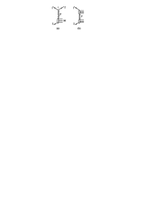
Figure 1: Single and double diffractive dissociation with a large rapidity gap represented by Pomeron exchange.

For example, for the (single) diffractive dissociation of particle 2 into a system of mass $M$, the rapidity gap between particle $1^{\prime}$ and the remaining hadrons is

$$\Delta y=\ln\left(\frac{s}{M^{2}}\right)=\ln\left(\frac{1}{x_{P}}\right),$$ (25)

where $x_{P}=1-x$ and $x=p_{1^{\prime}L}/(p_{1^{\prime}L})_{\rm max}$ is the Feynman $x$ variable of particle $1^{\prime}$. In general, the masses, $M_{i}$, of the diffractively excited states, produced in high energy $\sqrt{s}$ collisions, can be large. The only condition for diffractive dissociation is $M_{i}^{2}\ll s$.

In the Regge pole model, the cross section for the inclusive single diffractive dissociation process of Fig. 1(a) can be written in the form

$$x_{P}\frac{d^{2}\sigma}{dx_{P}\,dt}\ =\ \frac{(g_{11}(t))^{2}}{16\pi}|G_{P}(\Delta y,t)|^{2}\>\sigma_{P2}^{\rm tot}(M^{2},t)$$ (26)

where $t$ is the (square) of the 4-momentum transfer. The Green’s function (propagator) of the Pomeron is

$$G_{P}(\Delta y,t)={\mathcal{S}}\exp[(\alpha_{P}(t)-1)\Delta y],$$ (27)

where

$${\mathcal{S}}=\frac{1+\exp(-i\pi\alpha_{P}(t))}{\sin\pi\alpha_{P}(t)}$$ (28)

is the signature factor. The quantity $\sigma_{P2}^{\rm tot}(M^{2},t)$ can be considered as the Pomeron–particle 2 total interaction cross section [24]. This quantity is not directly observable. It is defined by its relation to the diffraction production cross section, (26). This definition is useful, however, because at large $M^{2}$, this cross section has the same Regge behavior as the usual total cross sections

$$\sigma_{P2}^{\rm tot}(M^{2},t)=\sum_{k}g^{k}_{22}(0)r^{k}_{PP}(t)\left(\frac{M^{2}}{s_{0}}\right)^{\alpha_{k}(0)-1}$$ (29)

where the $r^{k}_{PP}(t)$ is the triple-Reggeon vertex, which describes the coupling of two Pomerons to the Reggeon $k$.

Thus, in this region where the dissociating system has a large mass $M$, satisfying $s\gg M^{2}\gg m^{2}$, the inclusive diffractive cross section is described by the triple-Regge diagrams of Fig. 2.

Figure 2: Triple-Regge diagrams with $k=P$ or $f$ exchange describing high energy ($M^{2}\gg m^{2}$) Pomeron–particle 2 scattering.

Therefore, on inserting (29) into (26), we have

$$\frac{d^{2}\sigma}{dx\,dt}=\sum_{k}\Gamma_{k}(t)(1-x)^{\alpha_{k}(0)-2\alpha_{P}(t)}\left(\frac{s}{s_{0}}\right)^{\alpha_{k}(0)-1}.$$ (30)

The Pomeron and $f$ couplings to the proton, and the triple-Regge vertices $r^{P}_{PP},r^{f}_{PP}$, have been determined from analyses of experimental data on the diffractive production of particles in hadronic collisions (see the review in [8]). These couplings specify the factors $\Gamma_{k}(t)$ in (30).

In impact-parameter space, Regge amplitudes have a gaussian form at asymptotic energies. On the other hand, for inelastic diffraction we expect a peripheral form, which follows from unitarity in the $s$ channel picture. Note also that, since the Pomeron has intercept $\alpha_{P}(0)>1$, the cross sections of diffractive processes, (30), increase with energy faster than the total cross sections, and thus lead to a problem with unitarity. However, in Regge theory it is necessary to take into account, not only Regge poles, but also Regge cuts [25, 26], which correspond to the exchange of several Regge poles in the $t$ channel. These contributions restore the unitarity of the theory. For inelastic diffraction they lead to a peripheral form of the impact-parameter distributions and yield the appropriate energy dependence of the corresponding cross sections.

How is this realized in Regge theory? The explanation is based on a technique to evaluate Reggeon diagrams, introduced by Gribov [27], which allows the calculation of contributions of multi-Pomeron cuts in terms of Pomeron exchanges in the amplitudes of diffractive processes.

2.3 Compatibility of the $s$ and $t$ channel viewpoints:
Gribov’s Reggeon calculus and the AGK cutting rules

Gribov’s technique uses unitarity and analyticity of Reggeon–particle amplitudes, which follows from an analysis of Feynman diagrams [27]. For example the amplitude of two-Pomeron exchange in the $t$ channel (Fig. 3a) can be written as a sum over all diffractive intermediate states in the $s$ channel (Fig. 3b).

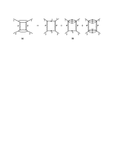
Figure 3: Two-Pomeron exchange in the $t$ channel expressed as the sum over all diffractive intermediate states in the $s$ channel. The crosses indicate that the particles are on the mass shell.

This result can be extended to multi-Pomeron exchanges in the $t$ channel. For the single ($s$) channel case, the summation of all elastic rescatterings leads to the well known eikonal formula with eikonal given by Fourier transform of the single-Pomeron-exchange diagram. For several diffractive channels the resulting amplitudes can be written in the matrix eikonal form of the type shown in (19) and (20). In this way a connection between the $s$ channel view of diffraction and Regge theory is established. Note that only for weak coupling can the Pomeron cuts be neglected, and just the first term in the expansion be retained. Another powerful tool for the calculation of, not only diffractive, but inelastic processes, which contribute to total cross section, is the AGK (Abramovsky, Gribov, Kancheli [28]) cutting rules. By applying these rules, it is possible to show the selfconsistency of the approach, which was absent in the pure Regge pole model. Consider a diagram where elastic scattering is mediated by the exchange of $k$ Pomerons. The AGK cutting rules specify the coefficients $c_{k}^{n}$ arising when $n$ of these Pomerons are cut. Recall that these Pomeron cut discontinuities give the corresponding inelastic contributions to $\sigma_{\rm tot}$. The terms with $n=0$ correspond to the diffractive cutting of the diagram (that is the cut is between the Pomeron exchanges, and not through the Pomerons themselves). These $n=0$ terms have the coefficients

$$c_{k}^{n=0}=2^{k-1}-1.$$ (31)

For two-Pomeron exchange, $k=2$, the coefficients are $+1$, $-4$, $+2$ according to whether $n=0$, 1 or 2 Pomerons are cut, respectively.

We illustrate the compatibility between the $s$ channel view of diffraction and the $t$ channel approach with multi-Pomeron cuts, using a simple example with two diffractive channels. In this case the $T$ matrix has the form (19)–(21) with function $\Omega_{0}$ given by

$$\Omega_{0}=\frac{(g_{pp}^{P})^{2}(s/s_{0})^{\Delta}}{4\pi B}e^{-b^{2}/4B}\ =\ \frac{(g^{P}_{pp})^{2}}{4\pi B}\exp\left(\Delta\ln\left(\frac{s}{s_{0}}\right)-\frac{b^{2}}{4B}\right),$$ (32)

where $B$ is the slope of the Pomeron amplitude,

$$B=\textstyle{\frac{1}{2}}B_{0}+\alpha_{P}^{\prime}\ln(s/s_{0}),$$ (33)

$g_{pp}^{P}$ is the coupling of the Pomeron to the proton, $s_{0}=1~{}{\rm GeV}^{2}$ and $\Delta\equiv\alpha_{P}(0)-1$. In practice, the value of $\gamma$ is about 0.4. Thus as a first approximation we may neglect higher powers of $\gamma$ in (19). The eikonal function $\Omega$ increases with energy as $(s/s_{0})^{\Delta}$, and at very high energies it follows, from (32) and (33), that $\Omega\gg 1$ for values of the impact parameter satisfying

$$b^{2}<R^{2}=4\alpha_{P}^{\prime}\Delta\ln^{2}(s/s_{0}).$$ (34)

As a consequence, the elastic and inelastic cross sections have strikingly different forms in impact parameter space. The elastic cross section is limited by the black disc bound, $\sigma_{\rm el}(b,s)=1$, up to $b\sim R$, after which it decreases rapidly. On the other hand, the inelastic cross section depends on the off-diagonal elements in (20) and (21),

$$\sigma_{12}(b,s)\simeq(\gamma\Omega_{0})^{2}e^{-\Omega_{0}},$$ (35)

and so is only non-zero in the peripheral region of the interaction, $b\sim R$. This example illustrates the general difference in the suppression of the elastic and inelastic channels due to multi-Pomeron exchanges, in agreement with $s$ channel unitarity.

Let us illustrate the self consistency of the Gribov technique for the evaluation of multi-Pomeron contributions, and the AGK cutting rules, in the simplest single-channel example. In this case the imaginary part of elastic amplitude in $b$ space has the eikonal form

$${\rm Im}\,T_{\rm el}(s,b)=\sum_{k=1}\frac{(-1)^{k+1}}{k!}\left(\frac{\Omega_{0}}{2}\right)^{k}=1-\exp(-\Omega_{0}/2).$$ (36)

By applying the AGK cutting rules [28] to each term of the series, it is possible to obtain for the diffractive (elastic) cross section [29]

$$\sigma_{\rm el}(s,b)=\sum_{k=1}\frac{(-1)^{k}}{k!}\left(\frac{\Omega_{0}}{2}\right)^{k}2(2^{k-1}-1)=(1-\exp(-\Omega_{0}/2))^{2}$$ (37)

and for inelastic cross section

$$\sigma_{\rm inel}(s,b)=\sum_{n=1}\frac{(\Omega_{0})^{n}}{n!}e^{-\Omega_{0}}=(1-\exp(-\Omega_{0})),$$ (38)

where $n$ is the number of cut Pomerons (with any number of uncut ones). It has a simple probabilistic interpretation. The second expression for $\sigma_{\rm inel}$ represents the whole probability, 1, minus the probability $\exp(-\Omega_{0})$ to have no inelastic interaction, whereas in the first expression each term $\Omega_{0}^{n}/n!$ represents the probability of $n$ inelastic interactions (where $n!$ accounts for the identity of the interactions) multiplied by $\exp(-\Omega_{0})$ which guarantees that there are no further inelastic interactions.

¿From (36)–(38) we see that, in the single channel case, we have

$$\sigma_{\rm el}(s,b)=({\rm Im}\,T_{\rm el}(s,b))^{2}$$ (39)

$$\sigma_{\rm el}(s,b)+\sigma_{\rm inel}(s,b)=\sigma_{\rm tot}(s,b)=2{\rm Im}\,T_{\rm el}(s,b),$$ (40)

as indeed it must be. Note that this self consistency could not be achieved if the series in multi-Pomeron rescatterings would be cut at some finite term. The consistency with $s$ channel unitarity can be proven for an arbitrary multichannel case.

It is also instructive to consider the situation with two Pomeron poles: soft $P_{\rm s}$ and hard $P_{\rm h}$. In the single channel case, a summation of $s$ channel rescatterings leads again to the eikonal formula [30] with

$$\Omega(s,b)=\Omega_{\rm s}(s,b)+\Omega_{\rm h}(s,b)$$ (41)

where the $\Omega_{i}(s,b)$ are the Fourier transforms of the $i$-Pomeron contributions. The hard Pomeron is usually related to the cross section of minijet production [31, 30], which rapidly increases with energy. It is interesting to note that the unitarization via eikonal formula described above leads to a rather weak influence of the hard component on the behaviour of the total cross sections, because this component becomes important only at energies when the soft component is large and the amplitudes at small impact parameters are close to the black disk limit. From the AGK cutting rules it is easy to prove that in this model, the cross section of a hard process (with any number $k\geq 1$ of hard interactions plus any number of soft inelastic interactions) is described by the eikonal expression with $\Omega=\Omega_{\rm h}$. This is the so-called self absorption theorem for processes with a given criterion [32]. In this case the criterion is the existence of at least one minijet. ¿From the above expression it is clear that such processes will dominate at very high energies, and that the mean number of minijets will be determined by $\Omega_{\rm h}$.

3 Diffractive eigenstates and parton configurations

The partonic picture of hadronic fluctuations mentioned above gives a new insight to processes of diffraction dissociation of hadrons. This picture naturally appears in QCD, where each hadron can be represented as a Fock state vector in terms of the quark and gluon degrees of freedom. At very high energies, these fluctuations have large lifetimes and have small variations during the time of the interaction. Thus configurations made of definite numbers of quarks, antiquarks and gluons with definite transverse coordinates can be considered as natural candidates for the eigenstates $|\phi_{k}\rangle$ of diffraction. Partonic models of diffraction were originally introduced in refs. [33, 34] and are now widely used within a QCD framework (for examples and references see [35]). In QCD, colourless configurations of small transverse size have small total interaction cross sections. Existence of such configurations leads to the phenomenon known as ‘color transparency’ [18, 19], which, in turn, leads to interesting effects in the diffractive interactions of hadrons and photons with nuclei. Existence of the diffractive eigenstates with substantially different interaction cross sections leads, according to (13), to large total cross sections of diffractive processes at high energies, which are close to the Pumplin bound (14). The distribution, $P(\sigma_{k})$, of cross sections $\sigma_{k}$ of the diffractive eigenstates $\phi_{k}$, has been determined from experimental data on diffractive processes for pions and protons in Refs. [36]. In the simplest 2-channel model, discussed in Section 2.1, the broad distribution $P(\sigma_{k})$ is approximated by 2 states with substantially different values of $\sigma_{k}$. In ref. [37] these states were related to the distributions of quarks and gluons with substantially different values of Bjorken $x$ (see also [38]). In Ref. [37] two models were considered. In the first model (model A) it was supposed that the valence quarks correspond to the small size component, while the sea quarks and gluons make up the large size component. In the second model (model B) the weights of the two components varied with $x$ in such a way that the small size component dominated at $x\sim 1$, while the large size component was dominant at small $x$.

Another interesting aspect of the partonic picture is the existence of partonic fluctuations with large masses, $M\gg m_{N}$, which correspond to multigluon configurations. In perturbative QCD, these are related to the BFKL Pomeron [39]. The elastic scattering of such states leads to the diffractive production of states of large mass, which in the Regge language corresponds to the triple-Pomeron interaction. The average mass of such states increases with energy, and at very high energies their role in inelastic diffractive processes becomes very important.

It was emphasized above, that at very high energies when elastic scattering becomes close to the black disk limit, there is a strong influence of different diffractive eigenstates on the properties of diffractive processes in the physical (hadronic) basis. In particular, there is a strong reduction of the cross section of large mass diffraction due to unitarity (multi-Pomeron rescatterings) effects. Below we will consider these effects for the diffractive production of large mass states, which contain a hard subprocess: the so-called hard diffractive processes.

4 Hard diffraction in $p\bar{p}$ ($pp$) and $pA$ collisions

The hard diffractive dissociation of hadrons or nuclei provides new possibilities for the investigation of diffraction dynamics. We illustrate this by discussing some typical reactions below. First, we describe a study of diffractive dijet production at the Tevatron, and then we proceed to make predictions for typical hard diffractive processes in proton–nuclear collisions that are accessible at RHIC. The possible relevance to diffraction at the LHC is mentioned.

4.1 Diffractive dijet production in $p\bar{p}$ collisions

Consider first the situation for dijet production in $pp$ ($p\bar{p}$) collisions. It is important that the single Pomeron exchange diagram of Fig. 4(a) can be calculated using QCD factorization for the hard processes, together with the distributions of partons in the proton and the Pomeron, denoted by $f_{i}^{p}$ and $f_{i}^{P}$ respectively.

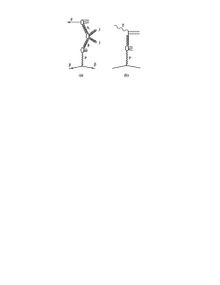
Figure 4: (a) The Born diagram for diffractive dijet production at the Tevatron, and (b)  the contribution to diffractive production at HERA driven by the gluonic component of the Pomeron. Notice that the lower parts of the diagrams are the same.

The latter ‘diffractive’ distributions can be extracted from an analysis of hard diffraction in deep inelastic scattering (Fig. 4(b)). Thus the cross section for diffractive dijet production, Fig. 4(a), may be written

$$\frac{d\sigma}{dt\,dx_{P}}=\sum_{i,k}\int F_{P}(x_{P},t)f_{i}^{P}(\beta,E_{T}^{2})f_{k}^{p}(x_{1},E_{T}^{2})\sigma_{ik}d\beta dx_{1}$$ (42)

where $\sigma_{ik}$ is the cross section for dijet production by partons with longitudinal momentum fractions $x_{1}$ and $\beta$ of the proton and Pomeron respectively, and $E_{T}$ is the transverse energy of the jets. $F_{P}$ is the Pomeron “flux factor”, which, according to (26), can be written in the form

$$F_{P}(x_{P},t)=\frac{(g_{pp}^{P}(t))^{2}}{(16\pi)x_{P}^{2\alpha_{P}(t)-1}}.$$ (43)

This approximation corresponds to the Ingelman–Schlein conjecture [40]. The existence of a hard scale provides the normalization of the Pomeron term.

In the previous sections we have emphasized the importance of multi-Pomeron contributions for diffractive particle production. For diffractive dijet production they correspond to the diagrams shown in Fig. 5.

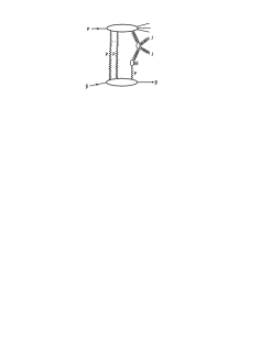
Figure 5: Multi-Pomeron contributions to diffractive dijet production at the Tevatron.

These diagrams lead to a strong violation of both Regge and hard factorization. Experimental data of CDF Collaboration at the Tevatron [41] clearly indicate the breaking of hard factorization in dijet production—the measured dijet cross section is an order of magnitude smaller than that predicted from (42) using HERA data for $f_{i}^{P}$. It is even more striking that the $\beta$ distribution for the produced dijets increases much faster as $\beta\rightarrow 0$, as compared with the expected behaviour of the partonic distributions. Both experimental observations can be reproduced in the model which takes into account the suppression of diffractive production at high energies due to multi-Pomeron exchanges. An essential feature of the model, which allows the reconciliation of the observed $\beta$ dependence with that expected from the partonic (mostly gluonic) distributions, is the relation between the size of the partonic fluctuation and the type (or the value of $x$) of the active parton. The suppression factor $S_{p}$ in this model can be written in the form

$$S_{p}=\frac{{\displaystyle\sum_{n}\int}d^{2}b\,|a_{pn}|^{2}|{\mathcal{M}}_{n}|^{2}\exp(-\Omega_{n}(s,b))}{{\displaystyle\sum_{n}\int}d^{2}b\,|a_{pn}|^{2}|{\mathcal{M}}_{n}|^{2}}\,,$$ (44)

where $|a_{pn}|^{2}$ is the probability of finding the partonic diffractive eigenstate $n\equiv|\phi_{n}\rangle$ in the proton $|p\rangle$, see (10), and $|{\mathcal{M}}_{n}|^{2}$ is the probability of producing the dijet system from the eigenstate $n$. It can depend on the type of the active parton $i$ and the value of its momentum, $x_{i}$ and $\vec{k}_{\perp i}$.

In Ref. [37] two eigenchannels were considered, $n=1,2$. It was argued that the channel with the smaller cross section (denoted the $S$ component) corresponds to valence quarks with $x\sim 1$, while the channel with the larger cross section is due to sea quarks and gluons and is concentrated at smaller values of $x$. This was denoted model A of the diffractive eigenstates. Of course, the model is oversimplified. There will be part of the valence component with large size, while on the other hand the gluons and sea quarks contribute to the small size component. An alternative model, model B, was introduced, in which the partonic distributions

$$f_{i}(x,E_{T}^{2})\ =\ (P_{i}^{S}+P_{i}^{L})f_{i}(x,E_{T}^{2})$$ (45)

with $i={\rm valence,\ sea,\ glue}$; where the large and small size projection operators have the forms

$$P_{i}^{L}=(1-x)^{n_{i}(Q^{2})},\qquad P_{i}^{S}=1-P_{i}^{L},$$ (46)

where the $n_{i}$ were chosen so that each component carries one half of the whole nucleon energy and one half of the number of valence quarks, see [37].

The functions $\Omega_{n}(s,b)$ in (44) have been parameterized in the form (see (23))

$$\Omega_{L}=(1+\gamma)\Omega_{0},\qquad\Omega_{S}=(1-\gamma)\Omega_{0},$$ (47)

with $\gamma=0.4$ [42]. In practice we use a more realistic parameterization of the $\Omega_{n}$, determined from the global description of total, elastic and soft diffractive production data [42]. In addition to the two-channel eikonal allowing for low mass diffraction, this analysis incorporated pion-loop insertions in the Pomeron trajectory, and high mass single- and double-diffractive dissociation via $s$ channel iterations of diagrams containing the triple-Pomeron interaction.

Interestingly, the order of magnitude suppression and the $\beta$ dependence of the prediction of the CDF dijet was well reproduced by both models A and B for the diffractive eigenstate, see Fig. 6, which was taken from Ref. [37].

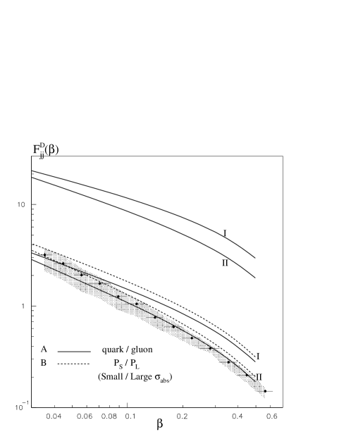
Figure 6: The four lower curves are the predictions for diffractive dijet production at the Tevatron obtained from two alternative sets of ‘HERA’ diffractive parton distributions I and II using models A (continuous curves) and B (dashed curves) to calculate the suppression factor $S_{p}$ of (44). Note that without the suppression factor the upper two curves in the plot would be obtained. The Tevatron dijet data (shown by the data points and shaded band) demonstrate the importance of including the shadowing corrections. The figure is taken from [37].

Note that, when the new fits to H1 diffractive data [43] are used in the approach of Ref. [37], even better agreement with CDF dijet data is achieved [44].

A further check of this general approach has been performed in Ref. [45]. There it was shown that the experimentally observed [46] breakdown of factorization in the ratio of the yields of dijet production in single diffractive and double-Pomeron-exchange processes is in good agreement with the expectations of the suppression factors obtained from the above-mentioned global analysis of diffractive phenomena [42].

4.2 Diffraction in proton–nuclear collisions

The suppression factors, analogous to (44), are much stronger for diffractive $p$-nuclear processes than for $pp$ (or $p\bar{p}$) collisions. They have a much richer structure. Their magnitudes, their $A$ and kinematic dependences are much more sensitive to the absorption cross sections of the proton partonic configurations of different transverse size, see, for example, [47]. Moreover, for collisions involving nuclei, $A$, there are more possibilities of diffractive dissociation. We will consider two types of proton–nuclear hard diffractive processes: the incoherent and coherent production of a massive system $h$ (accompanied by other particles, denoted by $X$)

$$pA\ \rightarrow\ Xh+Y_{A},$$ (48)

$$pA\ \rightarrow\ Xh+A,$$ (49)

as shown in Fig. 7.

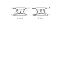
Figure 7: Multi-Pomeron exchange contributions to the incoherent and coherent diffractive production of a massive system $h$ in high energy proton–nuclear ($pA$) collisions. In (a) the nucleus $A$ has dissociated into a system $Y_{A}$ of nucleons, whereas in (b) it remains intact. The dots are to indicate any number of exchanged Pomerons, and/or interactions with any number of nucleons.

The observable system $h$ could be a dijet, a Drell–Yan pair or a heavy $q\bar{q}$ pair. For incoherent production, (48), the nucleus dissociates into a system of nucleons labelled $Y_{A}$. The momentum transfer is $t\sim 1/R_{p}^{2}$, where $R_{p}$ is the radius of the proton. On the other hand, in process (49) we have the coherent dissociation of the proton, while leaving the nucleus intact with very small momentum transfer, $t\sim 1/R_{A}^{2}$, where $R_{A}$ is the nuclear radius.

In the Born approximation for the interaction with a single nucleon, the cross section, integrated over $t$, of the second process is

$$\sigma^{\rm coh}(pA\rightarrow Xh+A)=\left.\frac{1}{B_{A}}\frac{d\sigma}{dt}\right|_{t=0}\simeq\frac{CA^{2}}{A^{2/3}}=CA^{4/3},$$ (50)

while the cross section of the incoherent process behaves as $\sigma(pA\rightarrow Xh+Y_{A})\sim A$. These $A$-dependences are drastically modified by multiple rescattering (multi-Pomeron exchanges), shown in Fig. 7.

The cross section for the incoherent hard diffraction on nuclei, process (48), in the Gribov–Glauber approach [48] is described by an analogous formula to that for $pp$ collisions,

$$\sigma(pA\rightarrow Xh+Y_{A})\ =\ \sum_{n}\int d^{2}b\,|a_{pn}|^{2}\sigma^{n}(pp\rightarrow h)T_{A}(b)\exp(-\sigma_{\rm abs}^{n}(s)T_{A}(b)),$$ (51)

where, as before, the sum is over the partonic diffractive eigenstates of the incoming proton, and $|a_{pn}|^{2}$ is the probability of finding eigenstate $n\equiv|\phi_{n}\rangle$ in the proton $|p\rangle$, see (10); $\sigma^{n}(pp\rightarrow h)$ is the corresponding cross section in proton–proton collisions for scattering through the $n^{\rm th}$ diffractive eigenstate, and $T_{A}(b)$ is the nuclear profile function (16). Here $\sigma_{\rm abs}^{n}(s)=\sigma_{\rm tot}^{n}-\sigma_{\rm el}^{n}$, where the cross sections are for proton–nucleon scattering at energy $\sqrt{s}$ through the $n^{\rm th}$ eigenstate, since elastic scattering does not change the kinematic structure of the process. Thus the nuclear suppression factor (sometimes called nuclear transparency) is

$$S_{A}^{\rm incoh}\ =\ \frac{\sigma(pA\rightarrow Xh+Y_{A})}{A\sigma(pp\rightarrow Xh)}\,,$$ (52)

where the denominator $\sigma(pp\rightarrow Xh)$ is the corresponding cross section for the diffractive production of the hard (massive) system $h$ in proton–nucleon collisions. Thus $S_{A}^{\rm incoh}$ is the extra suppression due solely to nuclear effects.

Coherent production on nuclei, process (49), is possible when the mass of the diffractively produced system, $M(hX)$, satisfies

$$M^{2}/s\ \ll\ 1/m_{p}R_{A},$$ (53)

where $\sqrt{s}$ is the proton–nucleon c.m. energy. Then the amplitude in impact parameter space is

$${\mathcal{M}}^{\rm coh}(pA\rightarrow Xh+A)\ =\ \sum_{n}a_{pn}{\mathcal{M}}^{n}(pp\rightarrow h)T_{A}(b)\exp\left(-\frac{\sigma_{\rm tot}^{n}}{2}T_{A}(b)\right),$$ (54)

where again the sum is over the diffractive eigenstates of the incoming proton. Here $\sigma_{\rm abs}^{n}=\sigma_{\rm tot}^{n}$, since even elastic scattering with $t\;\raisebox{-3.01385pt}{$\stackrel{{\scriptstyle\textstyle>}}{{\sim}}$}\;1/R_{A}^{2}$ will destroy the nucleus. Hence the total cross section of coherent diffractive production of $h$ is

$$\sigma^{\rm coh}(pA\rightarrow Xh+A)\ =\ \sum_{n}\int d^{2}b\,|a_{pn}|^{2}4\pi\left.\frac{d\sigma^{n}}{dt}\raisebox{6.88889pt}{$(pp\rightarrow h)$}\right|_{t=0}T_{A}^{2}(b)\exp(-\sigma_{\rm tot}^{n}T_{A}(b)).$$ (55)

We present below the results for the nuclear suppression factor for the coherent diffraction production of a system $h$ in the form

$$S_{A}^{\rm coh}=\left.\frac{d\sigma^{\rm coh}}{dt}\raisebox{6.88889pt}{$(pA\rightarrow Xh+A)$}\right|_{t=0}\ \Bigg{/}\ A^{2}\left.\frac{d\sigma}{dt}\raisebox{6.88889pt}{$(pp\rightarrow h)$}\right|_{t=0}.$$ (56)

Again this is the extra suppression arising solely from nuclear effects.

To be realistic, we present results for proton–nuclear ($pA$) collisions in the RHIC energy regime, $\sqrt{s}\simeq 300$ GeV, where $\sqrt{s}$ refers to the corresponding proton–nucleon c.m. energy. We use the same model that was employed to describe hard diffraction in $pp$ collisions [42]. We show results where the system $h$ is chosen to be Drell–Yan lepton pairs (which originate from $q\bar{q}$ annihilations), and also where $h$ is chosen to be either $c\bar{c}$ or $b\bar{b}$ pairs (which originate from $gg$ fusion). To be specific, we use a factorization scale $\mu^{2}=M^{2}_{\rm pair}$ where for Drell–Yan or $c\bar{c}$ production the mass of the pair is chosen to be $M_{\rm pair}=5$ GeV, while for beauty production we take $M_{b\bar{b}}=13$ GeV. The nuclear profile function, $T_{A}(b)$ of (16), was calculated using the standard Woods–Saxon form for $\rho(r)$ with the parameters determined from the electromagnetic form factors of nuclei [49]. In Figs. 8, 9 we show the nuclear suppression factors (52) and (56) as a function of the fraction of the longitudinal momentum of the incoming proton carried by the system $h$ ($=l^{+}l^{-}$, $c\bar{c}$ or $b\bar{b}$).

Figure 8: The extra nuclear suppression factors $S_{A}$ of (52) and (56) for the incoherent ($pA\rightarrow Xh+Y_{A}$) and coherent ($pA\rightarrow Xh+A$) diffractive production of a system $h$ carrying momentum fraction $x$ in proton scattering on $A=64$ (Cu) nuclei at corresponding proton–nucleon c.m. collision energy of $\sqrt{s}=300$ GeV. The dashed, dotted and continuous curves correspond to using a single-channel and double-channel (models A and B) eikonals respectively.

Figure 9: As in Fig. 8 but for proton collisions on $A=197$ (Au) nuclei.

Figs. 8 and 9 correspond to nuclei with $A=64$ and $A=197$ respectively. We see that, in general, the suppression due to nuclear effects is approximately a factor of 10 for $pA\rightarrow Xh+Y_{A}$ and a factor of 100 for $pA\rightarrow Xh+A$. The dashed lines in Figs. 8 and 9 correspond to the predictions of the one-channel eikonal model, which obviously cannot represent the different partonic configurations participating in the process. It therefore does not depend on the specific diffractively produced system $h$ or the momentum fraction $x$ that it carries. The other curves are the predictions of the two different two-channel eikonals introduced in Section 4.1 — the simple model A, which predicts the dotted curves, in which the valence quarks and the gluon + sea quarks are respectively associated with the small and large size diffractive eigenstates, $|\phi_{2}\rangle$ and $|\phi_{1}\rangle$ of (47); and model B, which predicts the continuous curves, with a more realistic partonic composition of the diffractive eigenstates.

For models A and B, we see that, in general, the nuclear suppression depends on $x$. For large $x$, where the small-size, low $\sigma_{\rm abs}$ component dominates, the suppression is less than that expected in the pure Glauber one-channel case with $\exp(-\langle\sigma\rangle T_{A})$. On the other hand, for smaller $x$, where more contribution comes from the large-size, higher $\sigma_{\rm abs}$ component, there is much more suppression. However, for charm (and beauty) production, model A predicts that the suppression is independent of $x$. The reason is that the gluons have all been assigned to a single component; moreover, as this component has $\sigma_{\rm abs}>\langle\sigma\rangle$, the suppression is larger than the single-channel prediction. In the more realistic model, model B, where the gluon is distributed between both eigenstates, the suppression is less and the $pA$ cross section larger, and moreover depends on $x$ — the large $x$ gluons are concentrated in the diffractive eigenstate with the small $\sigma_{\rm abs}$. On the other hand, Drell–Yan production originates from valence and sea quark annihilation and hence the difference between the predictions of models A and B is small.

In Fig. 9 we include the prediction for the nuclear suppression in diffractive $b\bar{b}$, as well as $c\bar{c}$, production. The only difference is that the scale is larger: $\mu=13$ GeV rather than 5 GeV. By comparing $c\bar{c}$ and $b\bar{b}$ production we see the results are not sensitive to the choice of scale. In Fig. 10 we present the $A$ dependence for the more realistic model B, for a large and a small value of $x$.

Figure 10: The $A$ dependence of the extra nuclear suppression factors $S_{A}$ of (52) and (56) for the diffractive production of a system $h$ in $pA$ collisions.

4.3 Comments on proton–nuclear diffractive processes

The above examples demonstrate the role that diffractive eigenstates (with different absorptive cross sections) play in the description of diffractive processes involving nuclei. In comparison with the over-simple single-channel Glauber approach, the nuclear suppression factors reveal an informative rich structure. They vary by more than a factor of two for the various hard diffractive processes.

Figures 8–10 are qualitatively valid for all energies. The suppression factors of nuclear origin, $S_{A}$, decrease only gradually with increasing energy due to the slow growth of $\sigma_{\rm tot}^{n}(s)$. Moreover, these nuclear shadowing effects for the interactions of protons with nuclei are similar to the suppression factors in proton–proton interactions at much higher energies [50]. (Recall that for both $pA$ and $pp$ collisions we refer to the proton–proton energy $\sqrt{s}$.) For instance, we see from Fig. 8 that the nuclear suppression factor in $p$-Copper collisions is $S_{A}\sim 0.1$ at RHIC energies of $\sqrt{s}=300$ GeV, which is comparable to the suppression $S_{p}$ in hard diffractive $pp$ collisions at the higher Tevatron energy, see for example, Fig. 6. This interesting correlation may be anticipated from the dependence of $S_{A}$ of (51) and (52) on the exponential of the product $-\sigma^{n}_{\rm tot}(s)T_{A}(b)$. Total cross sections increase with energy as $s^{\Delta}$ with $\Delta\sim 0.1$, while $T_{A}(b)\sim A^{1/3}$. Thus an increase of $s$ by two orders of magnitude is equivalent to an increase in $A$ by a factor $\sim 4$. Thus, since $S_{A}$ for $pA$ collisions with $A\sim 64$ at RHIC energies is comparable to $S_{p}$ for $pp$ collisions at the Tevatron ($s\sim(3$–$4)\times 10^{6}~{}{\rm GeV}^{2}$), we expect that $S_{p}$ at the LHC ($s\sim 2\times 10^{8}~{}{\rm GeV}^{2}$) will be close to $S_{A}$ for $pA$ collisions with $A\sim 197$ (see Fig. 9). So the observation of shadowing of hard diffractive processes on heavy nuclei at RHIC may serve as a guide to the size of the suppression factors $S_{p}$ which occur in similar processes in $pp$ collisions at the LHC energy. Of course, the $S_{p}$ factors can be calculated directly, but confirmation from a study of proton–nuclear scattering data at RHIC would be valuable. The $S_{p}$ factors need to be known, for example, in plans to identify New Physics phenomena in observations of such diffractive processes at the LHC.

5 Concluding remarks

Investigation of both soft and hard diffractive processes provides important information on the dynamics of strong interactions at high energies. With increasing energy the role of unitarity effects (which, in the Reggeon approach, materialise as multi-Pomeron exchange interactions) becomes more and more important. The association of eigenstates of the diffractive part of the $T$-matrix with definite partonic configurations leads to extra insight into the dynamics of diffractive processes in QCD. It allows one to determine the effective sizes of the partonic configurations in hard diffractive processes. The use of nuclear targets provides new possibilities for detailed studies of various aspects of both soft and hard diffractive processes. We have demonstrated that interesting information on the properties of partonic configurations can be obtained from a study of hard diffractive processes in $pA$-collisions at RHIC and LHC. A knowledge of diffraction dynamics, and especially of shadowing effects in $pp$ and $pA$ collisions, is important for predictions of the expected manifestations of New Physics in diffractive processes at proton colliders, see, for example, [3]. A well known example is double-diffractive Higgs boson production, see, for example, [22, 4, 51].

References

- [1] E.L. Feinberg and I.Ya. Pomeranchuk, Doklady Akad. Nauk SSSR 93, 439 (1953); Suppl. Nuovo Cimento v. III, serie X, 652 (1956).
- [2] M.G. Albrow and A. Rostovtsev, arXiv:hep-ph/0009336; and references therein.
- [3] V.A. Khoze, A.D. Martin and M.G. Ryskin, Eur. Phys. J. C23, 311 (2002).
- [4] A. De Roeck, V.A. Khoze, A.D. Martin, R. Orava and M.G. Ryskin, Eur. Phys. J. C25, 391 (2002); V.A. Khoze, A.D. Martin and M.G. Ryskin, Acta Phys. Polon. B33, 3473 (2002).
- [5] B.E. Cox, J.R. Forshaw and B. Heinemann, Phys. Lett. B540 (2002) 263.
- [6] M. Boonekamp, R. Peschanski and C. Royon, arXiv:hep-ph/0301244, and references therein.
- [7] M.L. Good and W.D. Walker, Phys. Rev. 120, 1857 (1960).
- [8] A.B. Kaidalov, Phys. Rept. 50, 157 (1979).
- [9] J. Pumplin, Physica Scripta 25, 191 (1982).
- [10] K. Goulianos, Phys. Rept. 101, 169 (1983).
- [11] H. Abramowicz and A. Caldwell, Rev. Mod. Phys. 71, 1275 (1999).
- [12] M. Wüsthoff and A.D. Martin, J. Phys. G25, R309 (1999).
- [13] A. Hebecker, Phys. Rept. 331, 1 (2000).
- [14] E.A. De Wolf, Acta Phys. Polon. B33, 4165 (2002).
- [15] J. Pumplin, Phys. Rev. D8, 2899 (1973).
- [16] L. Frankfurt, M. Strikman and M. Zhalov, arXiv:hep-ph/0211336.
- [17] I.P. Ivanov, N.N. Nikolaev, W. Schäfer, B.G. Zakharov and V.R. Zoller, arXiv:hep-ph/0212176.
- [18] G. Bertsch, S.J. Brodsky, A.S. Goldhaber and J.F. Gunion, Phys. Rev. Lett. 47, 297 (1981).
- [19] A.B. Zamolodchikov, B.Z. Kopeliovich and L.I. Ladidus, JETP Lett. 33, 595 (1981).
- [20] K.G. Boreskov, A.M. Lapidus, S.T. Sukhorukov and K.A. Ter-Martirosyan, Nucl. Phys. B40, 397 (1972).
- [21] E. Gotsman, E. Levin and U. Maor, Phys. Lett. B452, 387 (1999); Phys. Rev. D60, 094011 (1999), and references therein.
- [22] V.A. Khoze, A.D. Martin and M.G. Ryskin, Eur. Phys. J. C18, 167 (2000).
- [23] J. Alberi and J. Goggi, Phys. Rep. 74, 1 (1981).
- [24] A.B. Kaidalov, V.A. Khoze, Yu. F. Pirogov and N.L. Ter-Isaakyan, Phys. Lett. B45, 493 (1973); A.B. Kaidalov and K.A. Ter-Martirosyan, Nucl. Phys. B75, 471 (1974).
- [25] S. Mandelstam, Nuovo Cimento 30, 1148 (1963).
- [26] V.N. Gribov, I.Ya. Pomeranchuk and K.A. Ter-Martirosyan, Phys. Lett. 9, 269 (1964); Vad. Fiz. 2, 361 (1965).
- [27] V.N. Gribov, ZhETF 57, 654 (1967).
- [28] V.Abramovsky, V.N. Gribov and O.V. Kancheli, Sov. J. Nucl. Phys. 18, 308 (1974).
- [29] K.A. Ter-Martirosyan, Phys. Lett. B44, 377 (1973).
- [30] A. Capella, J. Kwieciński and J. Tran Thanh Van, Phys. Rev. Lett. 58, 2015 (1987).
- [31] L.V. Gribov, E.M. Levin and M.G. Ryskin, Phys. Rept. 100, 1 (1983).
- [32] R. Blankenbecler et al., Phys. Lett. B107, 106 (1981).
- [33] L. Van Hove and K. Fialkowski, Nucl. Phys. 107, 211 (1976).
- [34] H.I. Miettinen and J. Pumplin, Phys. Rev. D18, 1696 (1978).
- [35] K. Agreev et al. (FELIX), J. Phys. G28, R117 (2002).
-
[36]
G. Baym, B. Blättel, L.L. Frankfurt,
H. Heiselberg and M. Strikman, Phys. Rev. D47, 2761
(1993);
B. Blättel, G. Baym, L.L. Frankfurt and M. Strikman, Phys. Rev. Lett. 70, 896 (1993). - [37] A.B. Kaidalov, V.A. Khoze, A.D. Martin and M.G. Ryskin, Eur. Phys. J. C21, 521 (2001).
- [38] S.J. Brodsky, Tao Huang and G.P. Lepage, Proc. 9th SLCA Summer Inst. on Part. Phys., 87 (1981).
-
[39]
V.S. Fadin, E.A. Kuraev and L.N. Lipatov, Sov.
Phys. JETP 44, 443 (1976); 199 (1977);
I.I. Balitsky and L.N. Lipatov, Sov. J. Phys. 28, 822 (1978). - [40] G. Ingelman and P.E. Schlein, Phys. Lett. B152, 256 (1985).
- [41] T. Affolder et al. (CDF Collaboration), Phys. Rev. Lett. 84, 5043 (2000).
- [42] V.A. Khoze, A.D. Martin and M.G. Ryskin, Eur. Phys. J. C18, 167 (2000).
- [43] F.-P. Schilling, arXiv:hep-ph/0210027
- [44] V.A. Khoze, A.D. Martin and M.G. Ryskin, 31st HEP conf., ICHEP2002, Amsterdam, arXiv:hep-ph/0210094.
- [45] A.B. Kaidalov, V.A. Khoze, A.D. Martin and M.G. Ryskin, arXiv:hep-ph/0302091, Phys. Lett. (in press).
- [46] CDF Collaboration: T. Affolder et al., Phys. Rev. Lett. 85 (2000) 4215.
- [47] L. Frankfurt, G.A. Miller and M. Strikman, Phys. Rev. Lett. 71, 2859 (1993).
- [48] V.N. Gribov, Sov. Phys. JETP 29, 483 (1969); ibid. 30, 709 (1970).
- [49] A. Bohr and B.R. Mottelson, Nucl. Structure, v.1, W.A. Benjamin Inc., New York, Amsterdam, 1969.
- [50] A.B. Kaidalov, in Proc. of XXII Int. Symposium on “Multiparticle Dynamics”, Santiago de Compostela, 1992, ed. C. Pajares (World Scientific) p. 185.
- [51] V.A. Khoze, La Thuile 2001, Results and Perspectives in Particle Physics, p. 275; arXiv:hep-ph/0105224.