Abstract

The basic parameters of supersymmetric theories can be determined at future $e^{+}e^{-}$ linear colliders with high precision. We investigate in this report how polarisation measurements in $\tilde{\tau}$ and $\tilde{t}$ or $\tilde{b}$ decays to $\tau$ leptons and $t$ quarks plus neutralinos or charginos can be used to measure $\tan\beta$ (in particular for large values) and to determine the trilinear couplings $A_{\tau}$, $A_{t}$ and $A_{b}$ in sfermion pair production.

1 Introduction

If supersymmetry is realised in Nature [1, 2], a large number of low–energy parameters – masses, couplings and mixings – must be determined with high precision. This is necessary in order to investigate the mechanism breaking the symmetry and to reconstruct the fundamental theory eventually at a scale close to the Planck scale [3]. While the coloured SUSY partners are expected to be discovered at the hadron colliders Tevatron and LHC, future $e^{+}e^{-}$ linear colliders will provide a comprehensive picture of the weakly interacting, non–coloured particles [4, 5]. Moreover, the detailed analysis of their properties will be a central target of experiments at the linear colliders such as JLC/NLC/TESLA in the sub-TeV phase and as CLIC, a collider concept for extending the energy to the multi–TeV range.

The analysis program for the new particles has been developed in great detail for the mass parameters and mixings in the (non–coloured) sfermion and gaugino sectors [6]. It has been shown in particular how the SU(2)$\times$U(1) gaugino mass parameters $M_{2}$ and $M_{1}$, as well as the higgsino mass parameter $\mu$ can be extracted [7, 8]. However, while $\tan\beta$, the mixing parameter in the Higgs sector, can be measured well for moderate values in the chargino/neutralino sector, only bounds can be set on $\tan\beta$ if this parameter is large, i.e. $\tan\beta\raise 1.29167pt\hbox{$>$\kern-7.5pt\lower 4.30554pt\hbox{$\sim$}}10$, for simple mathematical reasons discussed later.

Several processes have been studied to measure $\tan\beta$ in different ways, complemented also by methods for measuring the trilinear $A$ couplings in the superpotential (see e.g. Ref. [9] and references therein). They include heavy Higgs boson decays to fermion and sfermion pairs, Higgs radiation off fermions and sfermions, and others. For this purpose some of us [10] made a detailed study of the tau polarisation in stau production. In this report we expand on this work and perform a comprehensive analysis of polarisation effects in sfermion decays to fermions plus neutralinos/charginos in $e^{+}e^{-}$ pair production of third-generation sfermions:

$$\begin{array}[]{llll}e^{+}e^{-}\to\tilde{\tau}_{i}\bar{\tilde{\tau}}_{j}\,,&&\tilde{\tau}_{i}\to\tau\tilde{\chi}^{0}_{k}&\quad\mbox{[}i,j=1,2;\ k=1,\ldots,4]\,,\\ e^{+}e^{-}\to\tilde{t}_{i}\bar{\tilde{t}}_{j}\,,&&\tilde{t}_{i}\to t\tilde{\chi}^{0}_{k}&\quad\mbox{[}i,j=1,2\ ;k=1,\ldots,4]\,,\\ e^{+}e^{-}\to\tilde{b}_{i}\bar{\tilde{b}}_{j}\,,&&\tilde{b}_{i}\to t\tilde{\chi}^{-}_{k}&\quad\mbox{[}i,j=1,2;\ k=1,2]\,.\end{array}$$ (4)

The $\tau$, $t$ fermions are longitudinally polarised in the 2–body decays of the scalar particles – the neutralino/chargino spin states are not measured.

Stau production has been proposed in Ref. [11] for investigating the properties of neutralinos. We do not only expand on this work but rather focus on the processes (4) as a means for measuring separately $\tan\beta$ and the trilinear couplings $A_{\tau}$, $A_{t}$, $A_{b}$ in the superpotential.

These parameters enter the off–diagonal $L/R$ element of the sfermion mass matrix in the combination

$$m_{LR}^{2}[\tilde{f}]=m_{f}\left[A_{f}-\mu\tan\beta(\cot\beta)\right]$$ (5)

for down (up)–type particles, respectively. The matrix element can be related directly to experimental observables – the physical masses $m_{\tilde{f}_{1}}$, $m_{\tilde{f}_{2}}$ and the mixing angle $\theta_{\tilde{f}}$:

$$m_{LR}^{2}[\tilde{f}]=\frac{1}{2}(m_{\tilde{f}_{1}}^{2}-m_{\tilde{f}_{2}}^{2})\sin 2\theta_{\tilde{f}}$$ (6)

While the sfermion masses can be determined accurately from decay spectra and from threshold scans, the mixing angles can be extracted from sfermion pair production.

The trilinear $A_{f}$ couplings and $\tan\beta$ can be disentangled by measuring the fermion polarisation in the decays $\tilde{f}\to f\tilde{\chi}$. In particular for large $\tan\beta$, the properties of the charginos and neutralinos – masses and mixings – are nearly independent of the specific value of this parameter as the gaugino mass matrices depend solely on $\cos 2\beta\simeq-1+2/\tan^{2}\beta$ and $\sin 2\beta\simeq 2/\tan\beta$. By contrast, the Yukawa couplings $f\tilde{f}\tilde{\chi}$ for down–type particles are of order $\cos^{-1}\beta\simeq\tan\beta$, with high sensitivity to large $\tan\beta$ – to the extent that the wave functions of the associated neutralinos and charginos possess non–negligible higgsino components. If this is not realised for the light gauginos, sfermion decays to heavy gauginos may be exploited in major parts of the supersymmetry parameter space wherever those decay channels are kinematically open and the corresponding decay branching ratios are sufficiently large.

The polarisation of fast moving $\tau$ particles affects the shape of the energy spectrum in decays like $\tau^{-}\to\nu_{\tau}\pi^{-}$ by angular–momentum conservation. For positive $\tau$ helicity, for instance, the pion is emitted preferentially in forward direction, carrying a large fraction of the $\tau$ energy while the spectrum is suppressed in the opposite direction, i.e. for soft $\pi$ energies. Another useful analyser is provided by the $\rho$ decay channel.

The polarisation of the top quark in decays $\tilde{b}\to t\tilde{\chi}^{-}$ and $\tilde{t}\to t\tilde{\chi}^{0}$ can be determined from the distribution of the quark jets in the hadronic top decays $t\to b\,+\,c\bar{s}$.

The report is organised as follows. In the next section we discuss the general analysis of the $\tilde{\tau}/\tau$ sector, followed in the third section by an experimental simulation for a specific large $\tan\beta$ reference point, $RP$, inferred from the Snowmass Point SPS1a [12]. In the fourth section we will present the analogous analysis for $\tilde{t}$ and $\tilde{b}$ decays including details on the measurement of the top quark polarisation in the decay final states.

2 The $\tilde{\tau}/\tau$ System

2.1 Masses and Mixing

Because of the large Yukawa couplings in the third generation, the left– and right–chiral stau states $\tilde{\tau}_{L}$ and $\tilde{\tau}_{R}$ mix to form mass eigenstates $\tilde{\tau}_{1}$ and $\tilde{\tau}_{2}$. The mass matrix in the L/R current basis can be written in the form

$${\cal M}^{2}_{\tilde{\tau}}=\left(\begin{array}[]{cc}M^{2}_{L}+m_{\tau}^{2}+D_{L}&m_{\tau}(A_{\tau}-\mu\tan\beta)\\ m_{\tau}(A_{\tau}-\mu\tan\beta)&M^{2}_{E}+m_{\tau}^{2}+D_{R}\end{array}\right)=\left(\begin{array}[]{cc}m_{LL}^{2}&m_{LR}^{2}\\ m_{LR}^{2}&m_{RR}^{2}\end{array}\right)$$ (11)

with the SU(2) doublet (singlet) mass parameter $M_{L}^{2}$ ($M_{E}^{2}$); the D–terms $D_{L}=(-{\frac{1}{2}}+\sin^{2}\theta_{W})\cos(2\beta)m^{2}_{Z}$ and $D_{R}=-\sin^{2}\theta_{W}\cos(2\beta)m^{2}_{Z}$; the trilinear $\tilde{\tau}_{R}$$\tilde{\tau}_{L}$$H_{1}$ stau–Higgs coupling $A_{\tau}$; the higgsino mass parameter $\mu$; and $\tan\beta=v_{2}/v_{1}$ the ratio of the two Higgs vacuum expectation values. The mass parameters $m_{LL}^{2}$, $m_{RR}^{2}$ are positive for $\tan\beta>1$, whereas $m_{LR}^{2}$ may carry either sign.

The two mass eigenvalues,

$$m_{\tilde{\tau}_{1,2}}^{2}=\frac{1}{2}\left[m_{LL}^{2}+m_{RR}^{2}\mp\sqrt{(m_{LL}^{2}-m_{RR}^{2})^{2}+4m_{LR}^{4}}\right],$$ (12)

are ordered in the sequence $m_{\tilde{\tau}_{1}}<m_{\tilde{\tau}_{2}}$ by definition. The mixing angle $\theta_{\tilde{\tau}}$ rotates the current states to the mass eigenstates,

$${\tilde{\tau}_{1}\choose\tilde{\tau}_{2}}=\left(\begin{array}[]{cc}\cos\theta_{\tilde{\tau}}&\sin\theta_{\tilde{\tau}}\\ -\sin\theta_{\tilde{\tau}}&\cos\theta_{\tilde{\tau}}\end{array}\right){\tilde{\tau}_{L}\choose\tilde{\tau}_{R}}$$ (13)

The stau mixing angle, defined on the interval $0\leq\theta_{\tilde{\tau}}<\pi$, is related to the diagonal and off–diagonal elements of the mass matrix,

$$\tan 2\theta_{\tilde{\tau}}=\frac{-2m_{LR}^{2}}{m^{2}_{RR}-m^{2}_{LL}}\,.$$ (14)

In reverse, the elements of the mass matrix can be expressed by the three characteristics of the state system, i.e. the two masses and the mixing angle:

$$m_{LL}^{2} = \frac{1}{2}({m^{2}_{\tilde{\tau}_{1}}+m^{2}_{\tilde{\tau}_{2}}})-\frac{1}{2}({m^{2}_{\tilde{\tau}_{2}}-m^{2}_{\tilde{\tau}_{1}}})\cos 2\theta_{\tilde{\tau}},$$ (15)

$$m_{RR}^{2} = \frac{1}{2}({m^{2}_{\tilde{\tau}_{1}}+m^{2}_{\tilde{\tau}_{2}}})+\frac{1}{2}({m^{2}_{\tilde{\tau}_{2}}-m^{2}_{\tilde{\tau}_{1}}})\cos 2\theta_{\tilde{\tau}},$$ (16)

$$m_{LR}^{2} = \frac{1}{2}(m_{\tilde{\tau}_{1}}^{2}-m^{2}_{\tilde{\tau}_{2}})\sin 2\theta_{\tilde{\tau}}.$$ (17)

Depending on the sign of $\cos 2\theta_{\tilde{\tau}}$, the SUSY mass parameter $m_{LL}^{2}$ is either smaller or larger than $m_{RR}^{2}$.

The two masses $m_{\tilde{\tau}_{1,2}}$ can be measured from the endpoints of the spectra in decay distributions and from threshold scans in $e^{+}e^{-}$ annihilation. The mixing angle $\theta_{\tilde{\tau}}$ can be determined from measurements of the production cross sections $e^{+}e^{-}\to\tilde{\tau}_{i}\tilde{\tau}_{j}$ [i,j=1,2]:

$$\sigma(e^{+}e^{-}\to\tilde{\tau}_{i}\tilde{\tau}_{j}) = \frac{8\pi\alpha^{2}}{3s}\lambda^{\frac{3}{2}}\Big{[}c_{ij}^{2}\,\frac{|\Delta(Z)|^{2}}{\sin^{4}2\theta_{W}}\,({\cal P}_{-+}L^{2}_{\tau}+{\cal P}_{+-}R^{2}_{\tau})$$ (18)

$$+\delta_{ij}\frac{1}{16}({\cal P}_{-+}+{\cal P}_{+-})+\delta_{ij}{c_{ij}}\,\frac{Re(\Delta(Z))}{2\sin^{2}2\theta_{W}}\,({\cal P}_{-+}L_{\tau}+{\cal P}_{+-}R_{\tau})\Big{]},$$

with $s$ denoting the cm energy squared. $\lambda^{\frac{1}{2}}$, with $\lambda=[1-(m_{\tilde{\tau}_{i}}+m_{\tilde{\tau}_{j}})^{2}/s][1-(m_{\tilde{\tau}_{i}}-m_{\tilde{\tau}_{j}})^{2}/s]$, is proportional to the velocity of the $\tilde{\tau}$ in the final state; the coefficient $\lambda^{3/2}$ in the cross section is characteristic for the $P$–wave suppression of pair-production of scalar particles at threshold in $e^{+}e^{-}$ annihilation. $\Delta(Z)=is/(s-m^{2}_{Z}+im_{Z}\Gamma_{Z})$ denotes the (renormalised) $Z$ propagator. The lepton/slepton couplings include the mixing angle,

$$c_{11/22}=\frac{1}{2}[L_{\tau}+R_{\tau}\pm(L_{\tau}-R_{\tau})\cos 2\theta_{\tilde{\tau}}]\,,$$ (19)

$$c_{12}=c_{21}=\frac{1}{2}(L_{\tau}-R_{\tau})\sin 2\theta_{\tilde{\tau}}\,,$$ (20)

with $L_{\tau}=\left(-\frac{1}{2}+\sin^{2}\theta_{W}\right)$ and $R_{\tau}=\sin^{2}\theta_{W}$ being the left/right chiral $Z$ charges of $\tau$. The electron/positron polarisation coefficients are defined as ${\cal P}_{-+}=(1-P_{e^{-}})(1+P_{e^{+}})$ and vice versa, with the first/second index denoting the $e^{-}/e^{+}$ helicity, and $P_{e^{-}}$, $P_{e^{+}}$ being the polarisation.

The measurement of one of the diagonal cross sections, for example, will determine $\cos 2\theta_{\tilde{\tau}}$ up to at most a single ambiguity. The ambiguity can be resolved by measuring the cross sections for two pairs 11 and 22, or by using polarised beams, or by varying the beam energy. The second method may be most useful in practice. The 12 cross section is generally small and therefore less useful in practice. Either of the other options will finally lead to a unique value of $\cos 2\theta_{\tilde{\tau}}$ from which the modulus $|\cos\theta_{\tilde{\tau}}|$ can be derived and, equivalently, $\theta_{\tilde{\tau}}$ up to the reflection $\theta_{\tilde{\tau}}\leftrightarrow\pi-\theta_{\tilde{\tau}}$. At the very end we are left with a sign ambiguity in the mixing parameter $\sin 2\theta_{\tilde{\tau}}$.

In summary. If the two masses $m_{\tilde{\tau}_{1,2}}$ and the mixing angle $|\cos\theta_{\tilde{\tau}}|$ have been determined, the off-diagonal element of the mass matrix is fixed up to a sign ambiguity. Thus the combination $(A_{\tau}-\mu\tan\beta)$ of the fundamental supersymmetric parameters $A_{\tau}$ and $\tan\beta$ can be evaluated up to a simple sign ambiguity solely from measurements of masses and cross sections.

2.2 ${\tau}$ Polarisation in $\tilde{\tau}$ Decays

To disentangle the parameters $A_{\tau}$ and $\tan\beta$ in the off–diagonal element of the mass matrix, the measurement of the $\tau$ (longitudinal) polarisation in the decays

$$\tilde{\tau}_{1}\to\tau\tilde{\chi}^{0}_{k}\quad\mbox{and}\quad\tilde{\tau}_{2}\to\tau\tilde{\chi}^{0}_{k}\quad[k=1,\ldots,4]$$ (21)

proves crucial. The $\tau$ polarisation depends in general on the mixing of the neutralino $\tilde{\chi}^{0}_{k}$ states and it can be expressed in terms of the Yukawa couplings ${\mathfrak{a}}^{L,R}_{ik}$ [11, 10]:

$$P_{\tilde{\tau}_{i}\to\tau\tilde{\chi}^{0}_{k}} = \frac{({\mathfrak{a}}_{ik}^{R})^{2}-({\mathfrak{a}}_{ik}^{L})^{2}}{({\mathfrak{a}}_{ik}^{R})^{2}+({\mathfrak{a}}_{ik}^{L})^{2}}\,,$$ (22)

with

$${\mathfrak{a}}_{1k}^{L,R} = \cos\theta_{\tilde{\tau}}{\mathfrak{a}}_{Lk}^{L,R}+\sin\theta_{\tilde{\tau}}{\mathfrak{a}}_{Rk}^{L,R}\quad\mbox{and}\quad{\mathfrak{a}}_{2k}^{L,R}=-\sin\theta_{\tilde{\tau}}{\mathfrak{a}}_{Lk}^{L,R}+\cos\theta_{\tilde{\tau}}{\mathfrak{a}}_{Rk}^{L,R},$$ (23)

where the scalar currents are defined by the interaction

$${\cal L}_{\tau}=\sum_{{i=1,2\atop k=1,\ldots,4}}\tilde{\tau}_{i}(\bar{\tau}_{R}{\mathfrak{a}}^{R}_{ik}+\bar{\tau}_{L}{\mathfrak{a}}^{L}_{ik})\tilde{\chi}^{0}_{k}$$ (24)

in the {gaugino; higgsino} basis $\{\tilde{B},\tilde{W}_{3};\tilde{H}_{1},\tilde{H}_{2}\}$:

$${\mathfrak{a}}_{Lk}^{R} = -\frac{g}{\sqrt{2}}\frac{m_{\tau}}{m_{W}\cos\beta}N_{k3}\quad\mbox{and}\quad{\mathfrak{a}}_{Rk}^{R}=-\frac{2g}{\sqrt{2}}N_{k1}\tan\theta_{W}\,,$$ (25)

$${\mathfrak{a}}_{Lk}^{L} = +\frac{g}{\sqrt{2}}[N_{k2}+N_{k1}\tan\theta_{W}]\quad\mbox{and}\quad{\mathfrak{a}}_{Rk}^{L}={\mathfrak{a}}_{Lk}^{R}.$$ (26)

The elements of the neutralino mixing matrix $N_{km}$ approach asymptotically a value independent of high $\tan\beta$ so that the coefficients in front of the ${\mathfrak{a}}^{R}_{Lk}$ and ${\mathfrak{a}}^{L}_{Rk}$ couplings are the key elements for our purpose. They are proportional to $\cos^{-1}\beta\simeq\tan\beta$ with a coefficient that depends only on parameters measured in the chargino/neutralino sector but is nearly independent of $\tan\beta$. To exploit the strong $\tan\beta$ dependence of ${\mathfrak{a}}^{R}_{Lk}$ and ${\mathfrak{a}}^{L}_{Rk}$, a significant higgsino component $\sim N_{k3}$ must be present in the neutralino wave function. Therefore $\tilde{\tau}_{i}$ [i=1,2] may be needed both to cover also the heavy neutralino decay channels. Unitarity ensures that at least one neutralino state with significant higgsino component in the wave function will be accessed. Since the coefficients of the key elements depend only on already measured parameters, we can predict a priori to what extent the method is useful for a particular decay process. The contour plots in Fig. 1 exemplify typical values of the higgsino parameter $N_{13}/N_{11}$ of $\tilde{\chi}^{0}_{1}$ versus $N_{33}/N_{31}$ of $\tilde{\chi}^{0}_{3}$ (both normalised to the bino component) in the $(\mu,M_{2})$ plane of the MSSM. [The constraint relation $M_{1}/M_{2}=\frac{5}{3}\tan\theta_{W}^{2}$ is adopted as an auxiliary assumption just for the sake of simplicity.] The kinks of the contour curves $N_{33}/N_{31}$ in Fig. 1b are caused by the exchange of the gaugino/higgsino mixing character of $\tilde{\chi}^{0}_{2}$ and $\tilde{\chi}^{0}_{3}$ as the corresponding mass eigenvalues change their ordering, cf. [14]. The reference point $RP$, given in Table 2, is marked by a star.

Figure 1: Contour plots in the $(M_{2},\mu)$ plane for the matrix elements $N_{13}/N_{11}$ and $N_{33}/N_{31}$. The reference point $RP$ is indicated by the blue star. The exclusion bounds are set to $m_{\tilde{\chi}^{0}_{1}}\geq 45$ GeV and $m_{\tilde{\chi}^{\pm}_{1}}\geq 103$ GeV.

Separating the neutralino mixing parameters from the relevant Yukawa couplings,

$$n_{g} = 1+\cot\theta_{W}\frac{N_{12}}{N_{11}}\,,$$ (27)

$$n_{h} = \cot\theta_{W}\frac{N_{13}}{N_{11}}\,,$$ (28)

gives rise to a transparent representation for the $\tau$ polarisation in $\tilde{\tau}_{1}\to\tau\tilde{\chi}^{0}_{1}$ decay:

$$P_{\tilde{\tau}_{1}\to\tau\tilde{\chi}^{0}_{1}} = \frac{(4-n_{g}^{2})-(4+n_{g}^{2}-2n_{h}^{2}\mu_{\tau}^{2}/\cos^{2}\beta)\cos{2\theta_{\tilde{\tau}}}+2(2+n_{g})n_{h}\sin{2\theta_{\tilde{\tau}}}\mu_{\tau}/\cos\beta}{(4+n_{g}^{2}+2n_{h}^{2}\mu_{\tau}^{2}/\cos^{2}\beta)-(4-n_{g}^{2})\cos{2\theta_{\tilde{\tau}}}+2(2-n_{g})n_{h}\sin{2\theta_{\tilde{\tau}}}\mu_{\tau}/\cos\beta}$$ (29)

with the abbreviation $\mu_{\tau}=m_{\tau}/m_{W}$. The formula is easily transcribed to other neutralino $\tilde{\chi}^{0}_{k}$ decays by adjusting the mixing coefficients $N_{1m}\Rightarrow N_{km}$. The transition to $\tilde{\tau}_{2}$ just requires flipping the signs of $\sin 2\theta_{\tilde{\tau}}$ and $\cos 2\theta_{\tilde{\tau}}$. Note that the polarisation itself is independent of the stau and neutralino masses.

3 A Specific Example

To study the experimental feasibility of measuring the parameters $\tan\beta$ and $A_{\tau}$, we have defined the reference point $RP$ in Table 2, that is motivated by the Snowmass point SPS1a [12]. The particle masses associated with the reference point $RP$ are collected in Table 2. The matrices diagonalizing the neutralino and chargino mass matrices are displayed in Tables 4 and 4. Note that the lightest neutralino $\tilde{\chi}^{0}_{1}$ state (and also the chargino $\tilde{\chi}^{+}_{1}$) has a significant higgsino component, $N_{13}$ (and $V_{12}$). In Table 5 the cross sections $\sigma(e^{+}e^{-}\to\tilde{\tau}_{i}\tilde{\tau}_{j})$ are listed for $\sqrt{s}=500$ GeV and $800$ GeV and various $e^{\pm}$ beam polarisations $P_{e^{-}}$ and $P_{e^{+}}$. The predicted $\tau$ polarisations and branching ratios of the decays ${\tilde{\tau}}_{1,\,2}\to\tau\tilde{\chi}^{0}_{k}$ are collected in Table 6.

For moderate values of $\tan\beta$, the polarisation is affected only indirectly by the wave-function through the gaugino mixing $n_{g}$ while the direct dependence on $\tan\beta$ through the Yukawa coupling is suppressed by the small mass ratio $\mu_{\tau}\sim 10^{-2}$. By contrast for ‘large $\tan\beta$’ in the range from 10 to 50, the gaugino and higgsino parameters, $n_{g}$ and $n_{h}$, are nearly independent of $\tan\beta$, cf. Ref. [8] and Appendix A, and the mixing angle $\theta_{\tilde{\tau}}$, with $\tan 2\theta_{\tilde{\tau}}\sim 2m_{\tau}\mu\tan\beta/M_{E,L}^{2}$, is expected to be still sufficiently away from the asymptotic value $\pi/4$. In this range, the polarisation is affected strongly by the Yukawa coupling $\sim\/{\cos^{-1}\beta}\simeq\tan\beta$ so that the polarisation measurement provides us with a new experimental method for determining large values of $\tan\beta$.

The Yukawa couplings can be proven as the origin for the sensitivity of the polarisation on $\tan\beta$ in $\tilde{\tau}_{1}\to\tau\tilde{\chi}^{0}_{1}$. This can be demonstrated by comparing the exact value of the $\tau$ polarisation $P=0.85$ with the approximate value derived for the gaugino and higgsino components $n_{g}$, $n_{h}$ of the neutralino in the asymptotic limit $\tan\beta\to\infty$: $P_{\infty}=0.86$.

Basic $RP$ Parameters
Gaugino Masses	$M_{1}$	99.1 GeV
	$M_{2}$	192.7 GeV
Higgs(ino) Parameters	$\mu$	140 GeV
	$\tan\beta$	20
Slepton Mass Parameters	$M_{L}$	300 GeV
	$M_{E}$	150 GeV
Squark Mass Parameters	$M_{Q}$	596 GeV
$3^{rd}$ generation	$M_{U}$	525 GeV
	$M_{D}$	617 GeV
Trilinear Couplings	$A_{\tau}$	$-254$ GeV
	$A_{b}$	$-773$ GeV
	$A_{t}$	$-510$ GeV

Table 1: Definition of the reference scenario $RP$ at the electroweak scale

Masses and Sfermion Mixing Angles
Neutralinos	$m_{\tilde{\chi}^{0}_{1}}$	78 GeV
	$m_{\tilde{\chi}^{0}_{2}}$	126 GeV
	$m_{\tilde{\chi}^{0}_{3}}$	152 GeV
	$m_{\tilde{\chi}^{0}_{4}}$	240 GeV
Charginos	$m_{\tilde{\chi}^{\pm}_{1}}$	110 GeV
	$m_{\tilde{\chi}^{\pm}_{2}}$	240 GeV
Staus	$m_{\tilde{\tau}_{1}}$	155 GeV
	$m_{\tilde{\tau}_{2}}$	305 GeV
Sbottoms	$m_{\tilde{b}_{1}}$	592 GeV
	$m_{\tilde{b}_{2}}$	624 GeV
Stops	$m_{\tilde{t}_{1}}$	497 GeV
	$m_{\tilde{t}_{2}}$	665 GeV
Sfermion Mixing Angles	$\theta_{{\tilde{\tau}}}$	1.492
	$\theta_{\tilde{b}}$	0.485
	$\theta_{\tilde{t}}$	0.987

Table 2: Physical masses and sfermion mixing angles in the reference scenario $RP$

Neutralino Mixing Matrix
	$N_{k1}$	$N_{k2}$	$N_{k3}$	$N_{k4}$
$\tilde{\chi}^{0}_{1}$	$-0.730$	$\ \ 0.248$	$-0.548$	$\ \ 0.325$
$\tilde{\chi}^{0}_{2}$	$\ \ 0.657$	$\ \ 0.488$	$-0.425$	$\ \ 0.386$
$\tilde{\chi}^{0}_{3}$	$\ \ 0.118$	$-0.161$	$-0.660$	$-0.724$
$\tilde{\chi}^{0}_{4}$	$-0.147$	$\ \ 0.821$	$\ \ 0.289$	$-0.470$

Table 3: Neutralino mixing matrix of $RP$

Chargino Mixing Matrix
	$V_{k1}$	$V_{k2}$		$U_{k1}$	$U_{k2}$
$\tilde{\chi}^{+}_{1}$	0.669	$-0.743$	$\tilde{\chi}^{-}_{1}$	$-0.408$	0.913
$\tilde{\chi}^{+}_{2}$	0.743	$0.669$	$\tilde{\chi}^{-}_{2}$	$0.913$	0.408

Table 4: Chargino mixing matrix of $RP$

	$\sqrt{s}=500$ GeV	$\sqrt{s}=800$ GeV
$(P_{e^{-}},P_{e^{+}})$	$\sigma(e^{-}e^{+}\to\tilde{\tau}_{1}\tilde{\tau}_{1})$	$\sigma(e^{-}e^{+}\to\tilde{\tau}_{1}\tilde{\tau}_{1})$	$\sigma(e^{-}e^{+}\to\tilde{\tau}_{2}\tilde{\tau}_{2})$	$\sigma(e^{-}e^{+}\to\tilde{\tau}_{1}\tilde{\tau}_{2})$
unpolarised	46.8 fb	29.4 fb	12.4 fb	0.06 fb
$(-0.8,0)$	24.0 fb	15.3 fb	19.1 fb	0.07 fb
$(+0.8,0)$	70.0 fb	43.6 fb	5.7 fb	0.05 fb
$(-0.8,+0.6)$	29.3 fb	18.9 fb	30.0 fb	0.11 fb
$(+0.8,-0.6)$	109.1 fb	68.3 fb	6.7 fb	0.07 fb

Table 5: Production cross sections of $e^{+}e^{-}\to{\tilde{\tau}}_{i}{\tilde{\tau}}_{j}$ for reference point $RP$ with polarised beams $(P_{e^{-}},\,P_{e^{+}})$. The cross sections for $\tilde{\tau}_{1}\tilde{\tau}_{2}$ production at $\sqrt{s}=500$ GeV are less than $0.1$ fb

$\tau$ Polarisations and ${\tilde{\tau}}$ Branching Ratios
	$\tilde{\tau}_{1}\to\tau\,\tilde{\chi}^{0}_{k}$		$\tilde{\tau}_{2}\to\tau\,\tilde{\chi}^{0}_{k}$
	$P_{\tau}$	${\cal B}_{{\tilde{\tau}}_{1}\to\tau\tilde{\chi}^{0}}$	$P_{\tau}$	${\cal B}_{{\tilde{\tau}}_{2}\to\tau\tilde{\chi}^{0}}$
$\tilde{\chi}^{0}_{1}$	$+0.85$	$0.78$	$+0.11$	$0.04$
$\tilde{\chi}^{0}_{2}$	$+0.76$	$0.12$	$-0.84$	$0.43$
$\tilde{\chi}^{0}_{3}$	—	—	$+0.72$	$0.05$
$\tilde{\chi}^{0}_{4}$	—	—	$-0.93$	$0.07$

Table 6: $\tau$ polarisations $P_{\tau}$ and branching ratios ${\cal B}_{\tilde{\tau}}$ of the decays $\tilde{\tau}_{1,2}\to\tau\tilde{\chi}^{0}_{k}$ for reference point $RP$

3.1 Summary of ${\tilde{\tau}}$ Parameter Measurements

The parameters of the ${\tilde{\tau}}$ system can be determined by measurements of the ${\tilde{\tau}}_{1},\ {\tilde{\tau}}_{2}$ masses and the mixing angle $\theta_{\tilde{\tau}}$ from which $\tan\beta$ and the trilinear coupling $A_{\tau}$ can be derived. Maximum sensitivity is achieved by proper choices of collision energy and beam polarisations, see Table 5. The following configurations with large rates are considered:

$$e^{+}_{L}e^{-}_{R} \to {\tilde{\tau}}_{1}{\tilde{\tau}}_{1}\ \qquad{\rm at}\ \sqrt{s}=500~{}\mathrm{GeV}\ ,$$ (30)

$$e^{+}_{R}e^{-}_{L} \to {\tilde{\tau}}_{2}{\tilde{\tau}}_{2}\ \qquad{\rm at}\ \sqrt{s}=800~{}\mathrm{GeV}\ .$$ (31)

Methods to determine particle masses include measurements of decay spectra and cross sections at the production thresholds. A Monte Carlo simulation of reaction (30), described in Appendix B, shows that the ${\tilde{\tau}}_{1}$ mass can be measured with an accuracy of $\delta m_{{\tilde{\tau}}_{1}}=0.5~{}\mathrm{GeV}$. Applying extrapolations of the present and previous studies [5] to ${\tilde{\tau}}_{2}{\tilde{\tau}}_{2}$ production at higher energies, one expects an uncertainty of $\delta m_{{\tilde{\tau}}_{2}}\simeq 2-3~{}\mathrm{GeV}$ on the ${\tilde{\tau}}_{2}$ mass.

The ${\tilde{\tau}}$ mixing angle $\theta_{\tilde{\tau}}$ is related to the total cross section, given by eqs. (18) – (20), and it is displayed in Fig. 2 for ${\tilde{\tau}}_{1}{\tilde{\tau}}_{1}$ production. The measurement of the cross section will not be limited by statistics, but rather by systematic effects with a typical error of $\delta\sigma/\sigma=3\,\%$. Using the theoretical prediction of $\sigma(e^{+}_{L}e^{-}_{R}\to{\tilde{\tau}}_{1}{\tilde{\tau}}_{1})=109~{}$fb at the Born level for $P_{e^{-}}=+80\%$, $P_{e^{+}}=-60\%$, with a statistical error of 1.0 fb and a systematical error of 3.3 fb, the mixing angle can be estimated to an accuracy of $\cos 2\theta_{\tilde{\tau}}=-0.987\pm 0.02\pm 0.06$ for an integrated luminosity of ${\cal L}=500~{}\mathrm{fb}^{-1}$, see Fig. 2. (The detailed simulation will be presented in Appendix B.)

Figure 2: Mixing angle $\cos 2\theta_{\tilde{\tau}}$ versus cross section $\sigma(e^{+}e^{-}\to{\tilde{\tau}}_{1}{\tilde{\tau}}_{1})$ at $\sqrt{s}=500~{}\mathrm{GeV}$ for beam polarisations $P_{e^{-}}=+0.8$ and $P_{e^{+}}=-0.6$ (green) and the unpolarised case (red) in the scenario $RP$. The vertical lines indicate the predicted cross sections. For unpolarised beams one observes a two-fold ambiguity in $\cos 2\theta_{\tilde{\tau}}$ (red dots); for polarised beams, however, only one solution lies in the allowed range (green dot).

The $\tau$ polarisation $P_{\tau}$ in ${\tilde{\tau}}$ decays can be measured from the shape of the energy spectra of hadronic decays, e.g. $\tau\to\pi\nu$. The energy distributions including the complete spin correlations for the final state $e^{+}_{L}e^{-}_{R}\to{\tilde{\tau}}_{1}{\tilde{\tau}}_{1}\to{\tilde{\tau}}_{1}^{\pm}+\pi^{\mp}\nu\tilde{\chi}^{0}_{1}$ have been calculated using CompHEP [16]. The polarised $\tau$ decays have been checked to agree with Tauola [17]. In a case study the accuracy of a polarisation measurement has been estimated by generating unweighted events at $\sqrt{s}=500~{}\mathrm{GeV}$ corresponding to an integrated luminosity of ${\cal L}=500~{}\mathrm{fb}^{-1}$. Taking all branching ratios into account and assuming an efficiency of $\varepsilon\simeq 0.30$ gives rise to about 3,300 decays $\tau\to\pi\nu$ with the pion energy spectrum shown in Fig. 3. The scaled pion energy distribution, $y_{\pi}=2E_{\pi}/\sqrt{s}$, is given [11] by

$$\frac{1}{\sigma}\frac{d\sigma}{dy_{\pi}} = \frac{1}{x_{+}-x_{-}}\begin{cases}(1-P_{\tau})\,\log\frac{x_{+}}{x_{-}}+2P_{\tau}\,y_{\pi}\,(\frac{1}{x_{-}}-\frac{1}{x_{+}})&\text{$0<y_{\pi}<x_{-}$}\\[4.30554pt] (1-P_{\tau})\,\log\frac{x_{+}}{y_{\pi}}+2P_{\tau}\,(1-\frac{y_{\pi}}{x_{+}})&\text{$x_{-}<y_{\pi}<x_{+}$}\end{cases}$$ (32)

where

$$x_{+/-} = \frac{m_{\tilde{\tau}}}{\sqrt{s}}\left(1-\frac{m_{\tilde{\chi}}^{2}}{m_{{\tilde{\tau}}}^{2}}\right)\frac{1\pm\beta}{\sqrt{1-\beta^{2}}}\ \mbox{ with }\ \beta\ =\ \sqrt{1-4m_{{\tilde{\tau}}}^{2}/s}\ .$$

A fit of the analytical formula to the generated spectrum gives a polarisation of $P_{\tilde{\tau}_{1}\to\tau\tilde{\chi}^{0}_{1}}=0.82\pm 0.03$, compatible with the theoretical value $P_{\tau}^{th}=0.85$ quoted in Table 6. From such a measurement of $P_{\tilde{\tau}_{1}\to\tau\tilde{\chi}^{0}_{1}}$ the inversion of expression (29) leads to a determination of $\tan\beta=22\pm 2$, as illustrated in Fig. 4. Note that the above approach neglects detector acceptances and resolution effects as well as backgrounds. It nevertheless provides a valuable estimate of the precision which can be achieved and which is later supported by detailed simulations described in Appendix B.

Figure 3: Pion energy spectrum $y_{\pi}=2\,E_{\pi}/\sqrt{s}$ from $\tau\to\pi\nu$ decays of $e^{+}_{L}e^{-}_{R}\to{\tilde{\tau}}^{+}_{1}{\tilde{\tau}}^{-}_{1}\to\tau^{+}\tilde{\chi}^{0}_{1}+\tau^{-}\tilde{\chi}^{0}_{1}$ production with $P_{e^{-}}=+0.8$, $P_{e^{+}}=-0.6$ at $\sqrt{s}=500~{}\mathrm{GeV}$, corresponding to ${\cal L}=500~{}\mathrm{fb}^{-1}$; reference scenario $RP$. The curve represents a fit to a $\tau$ polarisation of $P_{\tau}=0.82\pm 0.03$.

Figure 4: $\tan\beta$ versus $\tau$ polarisation $P_{{\tilde{\tau}}_{1}\to\tau\tilde{\chi}^{0}_{1}}$ for the reference scenario $RP$. The bands illustrate a measurement of $P_{\tau}=0.82\pm 0.03$ leading to $\tan\beta=22\pm 2$.

The off-diagonal elements of the mass matrix, eqs. (11) and (17), offer, in principle, the possibility to derive the trilinear coupling $A_{\tau}$ from the data:

$$A_{\tau}=\frac{m_{\tilde{\tau}_{1}}^{2}-m_{\tilde{\tau}_{2}}^{2}}{2m_{\tau}}\,\sin 2\theta_{\tilde{\tau}}+\mu\tan\beta\ .$$ (33)

In the reference scenario $RP$, with the trilinear coupling $A_{\tau}=-254~{}\mathrm{GeV}$, this method cannot be applied, however. The second term contributes to the total error with $\delta A_{\tau}^{(2)}=280~{}\mathrm{GeV}$. But the first term gives a huge error of $\delta A_{\tau}^{(2)}=2,400~{}\mathrm{GeV}$, even if only the statistical uncertainty in $\sin 2\theta_{{\tilde{\tau}}}=0.158\pm 0.125$ is taken into account. This is an artifact of the large ${\tilde{\tau}}$ mass splitting compared to $m_{\tau}$ and the small mixing, $\theta_{{\tilde{\tau}}}\simeq\pi/2$ in $RP$. The situation improves considerably for models with small mass differences and larger mixing. For example, a reduction of the slepton mass parameter $M_{L}=200~{}\mathrm{GeV}\,(\simeq m_{{\tilde{\tau}}_{2}})$, while the other $RP$ parameters are left unchanged, in particular $m_{{\tilde{\tau}}_{1}}=155~{}\mathrm{GeV}$ (cf. Table 2) leads to $\sin 2\theta_{{\tilde{\tau}}}=0.517\pm 0.033$ and a corresponding error of $\delta A_{\tau}^{(1)}=200~{}\mathrm{GeV}$, comparable to the contribution of $\delta A_{\tau}^{(2)}$ in eq. (33).

4 The $\tilde{t}$, $\tilde{b}\to t$ System

The analyses presented in the previous section can easily be expanded to squarks/quarks of the third generation. Three points should be noted for the transition from the lepton to the quark sector: i) Since squarks are significantly heavier than staus, the decays to heavier neutralino/chargino states $\tilde{\chi}^{0}_{3,4}$ and $\tilde{\chi}^{\pm}_{2}$ are possible which, in particular in mSUGRA–like scenarios, may carry a dominant higgsino component. ii) Decays of $b$ quarks cannot be exploited, as depolarisation effects during the fragmentation process $b\to B,\;B^{*}$ wash out the $b$ helicity signal. iii) Hadronic top decays can efficiently be used as analysers for the top polarisation in the decay $t\to bW\to b+c\bar{s}$ by tagging the $b$ and $c$ quarks while the flavour of the final $\bar{s}$ jet, which corresponds to the charged lepton in the leptonic $W$ decays of Ref. [18], need not be identified. These arguments lead us naturally to consider the channels

$$\tilde{t}_{i} \to t\,\tilde{\chi}^{0}_{k}\qquad[i=1,2;\ k=1,\ldots,4]\ ,$$ (34)

$$\tilde{b}_{i} \to t\,\tilde{\chi}^{-}_{k}\qquad[i=1,2;\ k=1,2]\ .$$ (35)

From the off–diagonal elements of the $\tilde{t}$ and $\tilde{b}$ mass matrices

$$m_{LR}^{2}[\tilde{t}] = \frac{1}{2}(m_{\tilde{t}_{1}}^{2}-m_{\tilde{t}_{2}}^{2})\sin 2\theta_{\tilde{t}}\ =\ m_{t}(A_{t}-\mu\cot\beta)\ ,$$ (36)

$$m_{LR}^{2}[\tilde{b}] = \frac{1}{2}(m_{\tilde{b}_{1}}^{2}-m_{\tilde{b}_{2}}^{2})\sin 2\theta_{\tilde{b}}\ =\ m_{b}(A_{b}-\mu\tan\beta)\$$ (37)

combinations of $\tan\beta$ and the trilinear couplings $A_{t}$ and $A_{b}$ can be determined. The sensitivity to $\tan\beta$ in the stop sector is low for large $\tan\beta$, so that access is provided primarily to $A_{t}$. Conversely, the pattern in the sbottom sector is quite analogous to the stau sector.

With the couplings defined in analogy to eq. (24)

$${\cal L}_{q} = \sum_{{i,k}}\tilde{q}_{i}(\bar{t}_{R}{\mathfrak{b}}^{R}_{ik}+\bar{t}_{L}{\mathfrak{b}}^{L}_{ik})\tilde{\chi}_{k},$$ (38)

the (longitudinal) polarisation formulae are modified slightly owing to the large top mass in the final state:

$$P_{\tilde{q}_{i}\to t{\tilde{\chi}}_{k}}=\frac{[({\mathfrak{b}}_{ik}^{R})^{2}-({\mathfrak{b}}_{ik}^{L})^{2}]\,f_{1}}{[({\mathfrak{b}}_{ik}^{R})^{2}+({\mathfrak{b}}_{ik}^{L})^{2}]-2{\mathfrak{b}}_{ik}^{R}{\mathfrak{b}}_{ik}^{L}\,f_{2}}.$$ (39)

The additional coefficients $f_{1}$ and $f_{2}$, cf. eq. (22), purely kinematical in origin, are given by

$$f_{1}\ =\ m_{t}\,\frac{(p_{\tilde{\chi}}\,s_{t})}{(p_{t}\,p_{\tilde{\chi}})}\ ,\qquad f_{2}\ =\ m_{t}\,\frac{m_{\tilde{\chi}}}{(p_{t}\,p_{\tilde{\chi}})}\ ,$$ (40)

where $m_{t}$, $p_{t}$, $s_{t}$ denote the mass, momentum and longitudinal spin vector of the decaying top quark, and $p_{\tilde{\chi}}$ the momentum of the neutralino. These coefficients can be written in the $t$ rest frame as

$$f_{1} = \frac{\lambda^{\frac{1}{2}}(m_{\tilde{q}}^{2},m_{t}^{2},m_{\tilde{\chi}}^{2})}{m_{\tilde{q}}^{2}-m_{t}^{2}-m_{\tilde{\chi}}^{2}}\ ,\qquad f_{2}\ =\ \frac{2m_{t}m_{\tilde{\chi}}}{m_{\tilde{q}}^{2}-m_{t}^{2}-m_{\tilde{\chi}}^{2}}\ .$$ (41)

They approach $f_{1}\to 1$ and $f_{2}\to 0$ for small decay fermion masses, leading back to eq. (29).

The differential distribution of the $\bar{s}$ jet in the top decay is given by

$$\frac{1}{\Gamma}\frac{d\Gamma}{d\cos\theta^{*}_{s}} = \frac{1}{2}(1+P_{\tilde{q}_{i}\to t\tilde{\chi}_{k}}\cos\theta^{*}_{s}),$$ (42)

where $\theta^{*}_{s}$ is the angle between the $\bar{s}$ quark from the $W$-boson in the $t$ decay and the primary sfermion $\tilde{t}_{i}$ ($\tilde{b}_{i}$) in the top rest frame.

i) $\tilde{t}\to t$ Transition
The polarisation of the $t$ quark in this decay process is explicitly given by

$$P_{\tilde{t}_{1}\to t\tilde{\chi}^{0}_{k}} = \frac{{\cal F}^{N}f_{1}}{{\cal F}^{D_{1}}-{\cal F}^{D_{2}}f_{2}}\ ,$$ (43)

where the coefficients of the numerator ${\cal F}^{N}$ and denominator ${\cal F}^{D_{1}}$ are known from the massless case, only with charge $e_{t}=2/3$, Yukawa coupling $Y_{t}=\mu_{t}/(\sqrt{2}\sin\beta)$ and top–type electro-weak isospin $I_{3L}^{t}=1/2$ adapted properly:

$${\cal F}^{N} = {I_{3L}^{t}}^{2}({n_{g}}-2)^{2}+2e_{t}I_{3L}^{t}(n_{g}-2)+\sqrt{2}\sin{2\theta_{\tilde{t}}}Y_{t}{n_{h}^{t}}[2e_{t}+I_{3L}^{t}(n_{g}-2)]$$ (45)

$$+\cos{2\theta_{\tilde{t}}}[{I_{3L}^{t}}^{2}(n_{g}-2)^{2}+2e_{t}I_{3L}^{t}(n_{g}-2)+2e_{t}^{2}-Y_{t}^{2}{n_{h}^{t}}^{2}]$$

$$= 9{n_{g}}^{2}-12n_{g}-12+(12+18n_{g}){n_{h}^{t}}\sin{2\theta_{\tilde{t}}}\mu_{t}/\sin\beta$$

$$+(9n_{g}^{2}-12n_{g}+20-18{n_{h}^{t}}^{2}\mu_{t}^{2}/\sin^{2}\beta)\cos{2\theta_{\tilde{t}}}$$

$${\cal F}^{D_{1}} = {I_{3L}^{t}}^{2}(n_{g}-2)^{2}+2e_{t}I_{3L}^{t}(n_{g}-2)+2e_{t}^{2}+Y_{t}^{2}{n_{h}^{t}}^{2}+\sqrt{2}\sin{2\theta_{\tilde{t}}}Y_{t}I_{3L}^{t}n_{h}^{t}(n_{g}-2)$$ (47)

$$+\cos{2\theta_{\tilde{t}}}[{I_{3L}^{t}}^{2}(n_{g}-2)^{2}+2e_{t}I_{3L}^{t}(n_{g}-2)]$$

$$= 9n_{g}^{2}-12n_{g}+20+18{n_{h}^{t}}^{2}\mu_{t}^{2}/\sin\beta^{2}+18n_{h}^{t}(n_{g}-2)\sin{2\theta_{\tilde{t}}}\mu_{t}/\sin\beta$$

$$+(9n_{g}^{2}-12n_{g}-12)\cos{2\theta_{\tilde{t}}}$$

$${\cal F}^{D_{2}} = \sqrt{2}Y_{t}I_{3L}^{t}n_{h}^{t}(n_{g}-2)-\sin{2\theta_{\tilde{t}}}[2e_{t}^{2}+2e_{t}I_{3L}^{t}(n_{g}-2)-Y_{t}^{2}{n_{h}^{t}}^{2}]$$ (49)

$$+\sqrt{2}\cos{2\theta_{\tilde{t}}}Y_{t}n_{h}^{t}[2e_{t}+I_{3L}^{t}(n_{g}-2)]$$

$$= 18n_{h}^{t}(n_{g}-2)\mu_{t}/\sin\beta-(24n_{g}-16-18{n_{h}^{t}}^{2}\mu_{t}^{2}/\sin^{2}\beta)\sin{2\theta_{\tilde{t}}}$$

$$+n_{h}^{t}(12+18n_{g})\cos{2\theta_{\tilde{t}}}\mu_{t}/\sin\beta$$

The abbrevations $n_{g}$, $n_{h}^{t}$ for the gaugino and higgsino components are given by

$$n_{g} = 1+\cot\theta_{W}\frac{N_{k2}}{N_{k1}}\ ,$$ (50)

$$n_{h}^{t} = \cot\theta_{W}\frac{N_{k4}}{N_{k1}}\ .$$ (51)

The expression for the $t$ polarisation in the $\tilde{t}_{2}$ decay can be derived from eq. (43) by changing the sign of all terms $\sim\sin 2\theta_{\tilde{t}}$ and $\sim\cos 2\theta_{\tilde{t}}$ in eqs. (45)–(49) .

ii) $\tilde{b}\to t$ Transition
With the appropriate couplings inserted, the polarisation of the top quark in the decays $\tilde{b}_{i}\to t\tilde{\chi}^{\pm}_{k}$ can be written equivalently to eq. (43):

$$P_{\tilde{b}_{1}\to t\tilde{\chi}^{\pm}_{k}} = \frac{{\cal G}^{N}f_{1}}{{\cal G}^{D_{1}}-{\cal G}^{D_{2}}f_{2}}\ .$$ (52)

The coefficients of the numerator ${\cal G}^{N}$ and denominator ${\cal G}^{D_{1}}$ and ${\cal G}^{D_{2}}$ are given by

$${\cal G}^{N} = -{c_{h}^{+}}^{2}\mu_{t}^{2}/\sin^{2}\beta+{c_{h}^{-}}^{2}\mu_{b}^{2}/\cos^{2}\beta+2-(2\sqrt{2}c_{h}^{-}\mu_{b}/\cos\beta)\sin 2\theta_{\tilde{b}}$$ (53)

$$-({c^{+}_{h}}^{2}\mu_{t}^{2}/\sin^{2}\beta+{c^{-}_{h}}^{2}\mu_{b}^{2}/\cos^{2}\beta-2)\cos 2\theta_{\tilde{b}}\ ,$$

$${\cal G}^{D_{1}} = {c_{h}^{+}}^{2}\mu_{t}^{2}/\sin^{2}\beta+{c_{h}^{-}}^{2}\mu_{b}^{2}/\cos^{2}\beta+2-(2\sqrt{2}c_{h}^{-}\mu_{b}/\cos\beta)\sin 2\theta_{\tilde{b}}$$ (54)

$$+({c^{+}_{h}}^{2}\mu_{t}^{2}/\sin^{2}\beta-{c^{-}_{h}}^{2}\mu_{b}^{2}/\cos^{2}\beta+2)\cos 2\theta_{\tilde{b}}\ ,$$

$${\cal G}^{D_{2}} = -c_{h}^{+}(1+\cos 2\theta_{\tilde{b}})2\sqrt{2}\mu_{t}/\sin\beta+c_{h}^{+}c_{h}^{-}4\sin 2\theta_{\tilde{b}}\mu_{t}\mu_{b}/\sin 2\beta\ ,$$ (55)

where $c_{h}^{+}$ and $c_{h}^{-}$ are ratios of $U$ and $V$ mixing-matrix elements,

$$c_{h}^{+} = V_{k2}/U_{k1}\ ,$$ (56)

$$c_{h}^{-} = U_{k2}/U_{k1}\ .$$ (57)

The components of the chargino mixing matrix in the high $\tan\beta$ approximation read:

$$U_{12} = \phantom{+}U_{21}=\sqrt{W+M_{2}^{2}-\mu^{2}+2m_{W}^{2}}/\sqrt{2W}\ ,$$ (58)

$$U_{11} = -U_{22}=-{\rm sign}(\mu)\sqrt{W-M_{2}^{2}-\mu^{2}+2m_{W}^{2}}/\sqrt{2W}\ ,$$ (59)

$$V_{12} = -V_{21}=-{\rm sign}(M_{2})\sqrt{W+M_{2}^{2}-\mu^{2}-2m_{W}^{2}}/\sqrt{2W}\ ,$$ (60)

$$V_{11} = \phantom{+}V_{22}=\sqrt{W-M_{2}^{2}-\mu^{2}-2m_{W}^{2}}/\sqrt{2W}\hskip 14.22636pt$$ (61)

with $W=\sqrt{(M_{2}^{2}+\mu^{2}+2m_{W}^{2})^{2}-4M_{2}^{2}\mu^{2}}$. The explicit expression for the $t$ polarisation in the decay $\tilde{b}_{2}\to t\tilde{\chi}^{\pm}_{k}$ can be derived from eq. (52) by changing in eqs. (53)–(55) the sign in the terms $\sim\cos 2\theta_{\tilde{b}}$ and $\sim\sin 2\theta_{\tilde{b}}$.

4.1 A Study of $t$ Polarisation

Since the $t$ polarisation in the process $\tilde{t}_{i}\to t\tilde{\chi}^{0}_{k}$ depends on $1/\sin\beta$, eqs. (45)–(49), it is only weakly sensitive to large $\tan\beta$. By contrast, the decay $\tilde{b}_{1}\to t\tilde{\chi}^{\pm}_{1}$ can be used indeed to measure $\tan\beta$. A feasibility study of the reaction

$$e^{+}_{L}e^{-}_{R} \to {\tilde{b}}_{1}\bar{\tilde{b}}_{1}\ \to\ t\tilde{\chi}_{1}^{\pm}+\bar{t}\tilde{\chi}_{k}^{\mp}\quad\$$ (62)

has been performed at $\sqrt{s}=1.9~{}\mathrm{TeV}$ within the reference scenario $RP$. The cross section amounts to $\sigma_{{\tilde{b}}_{1}{\tilde{b}}_{1}}=10~{}\mathrm{fb}$ assuming beam polarisations of $P_{e^{-}}=+0.80$ and $P_{e^{+}}=-0.60$.

The top polarisation measurement requires the reconstruction of the $t$ system and of the direction of the primary squark ${\tilde{b}}_{1}$. If no other particles except the neutralinos escape detection and all SUSY particle masses are known (as assumed in the present study), it is possible to reconstruct the momenta of both $\tilde{\chi}^{0}_{1}$ kinematically. The ${\tilde{b}}_{1}$ directions can then be determined up to a twofold ambiguity, where the correct solution gives the expected angular distribution $\propto\sin\theta^{2}_{\tilde{b}_{1}}$ while the false solution contributes uniformly in $\cos\theta_{\tilde{b}_{1}}$. For a distribution measured with respect to the ${\tilde{b}}_{1}$ direction, like the strange quark in the top decay of eq. (42), the ambiguity can be resolved on a statistical basis by subtracting the ‘wrong’ solution (e.g. via a Monte Carlo simulation). Therefore the following decay chains of reaction (62) have been considered:

$${\tilde{b}}_{1}^{(1)} \to \ \ t\tilde{\chi}_{1}^{\pm},\,\qquad t\to b\,W\to b\,c\bar{s},\ \quad\tilde{\chi}_{1}^{\pm}\to q\bar{q}^{\prime}\,\tilde{\chi}^{0}_{1}\qquad\qquad\quad\,{\cal B}^{(1)}=0.076\ ,$$ (63)

$${\tilde{b}}_{1}^{(2)} \to \begin{cases}t\tilde{\chi}_{1}^{\pm},\qquad t\to b\,W\to b\,q\bar{q}^{\prime},\quad\tilde{\chi}_{1}^{\pm}\to q\bar{q}^{\prime}\,\tilde{\chi}^{0}_{1}&\quad{\cal B}^{(2)}=0.152\ ,\\[4.30554pt] t\tilde{\chi}_{2}^{\pm},\qquad t\to b\,W\to b\,q\bar{q}^{\prime},\quad\tilde{\chi}_{2}^{\pm}\to q\bar{q}^{\prime}\,(W/Z)\,\tilde{\chi}^{0}_{1}&\quad{\cal B}^{(3)}=0.180\ ,\end{cases}$$ (64)

where the first sequence contains the decay of interest and the ${\cal B}^{(i)}$ denote the combined branching ratios. The ${\tilde{b}}_{1}$ branching ratios to charginos are ${\cal B}({\tilde{b}}_{1}\to t\tilde{\chi}^{\pm}_{1})=0.36$ and ${\cal B}({\tilde{b}}_{1}\to t\tilde{\chi}^{\pm}_{2})=0.30$. The large number of combinatorics can be efficiently reduced by requiring flavour identification – two bottom jets from top decays and at least one charm jet from $W$ decays – and applying additional kinematic constraints on the reconstruction of $W$ masses, top masses and chargino $\tilde{\chi}_{1}^{\pm}$ or $\tilde{\chi}_{2}^{\pm}$ masses.

The program CompHEP [16] has been used to calculate the exact decay distributions of the 5-particle final state $e^{+}e^{-}\to{\tilde{b}}_{1}+t\,\tilde{\chi}_{1}^{\pm}\to{\tilde{b}}_{1}+bc\bar{s}\,\tilde{\chi}_{1}^{\pm}$. Flavour tagging efficiencies for bottom and charm jets of $\varepsilon_{b}=0.85$ and $\varepsilon_{c}=0.5$ with reasonable purities ($\sim 0.8$) have been assumed [5]. With an integrated luminosity of ${\cal L}=2,000~{}\mathrm{fb}^{-1}$ one expects $N=2\,{\cal B}^{(1)}\,({\cal B}^{(2)}+{\cal B}^{(3)})\,\sigma_{{\tilde{b}}_{1}{\tilde{b}}_{1}}\,\varepsilon\,{\cal L}\simeq 330$ reconstructed ${\tilde{b}}_{1}\to t\tilde{\chi}_{1}^{\pm}$ decays. The generated angular distribution $\cos\theta^{*}_{s}$, where $\theta^{*}_{s}$ is the angle between the $\bar{s}$ quark and the primary ${\tilde{b}}_{1}$ in the top rest frame, is presented in Fig. 5. A fit to the top polarisation, given by eq. (42), yields $P_{t}=-0.44\pm 0.10$, which is consistent with the input value of $P_{t}^{th}=-0.38$. From such a measurement one can derive $\tan\beta=17.5\pm 4.5$, as illustrated in Fig. 6.

Figure 5: Angular distribution in $\cos\theta^{*}_{s}$, with $\theta^{*}_{s}$ being the angle between the ${\tilde{b}}_{1}$ and $\bar{s}$ partons in the top rest frame of $t\to b\,c\bar{s}$ decays from $e^{+}_{L}e^{-}_{R}\to{\tilde{b}}_{1}{\tilde{b}}_{1}\to t\tilde{\chi}_{1}^{\pm}+{\tilde{b}}_{1}$ production at $\sqrt{s}=1.9~{}\mathrm{TeV}$. The histogram corresponds to ${\cal L}=2,000~{}\mathrm{fb}^{-1}$, the line represents a fit to a top polarisation of $P_{t}=-0.44\pm 0.10$.

Figure 6: $\tan\beta$ as a function of top polarisation $P_{{\tilde{b}}_{1}\to t\tilde{\chi}_{1}^{\pm}}$ for reference scenario $RP$. The bands indicate the results of a simulation with $P_{t}=-0.44\pm 0.10$ leading to $\tan\beta=17.5\pm 4.5$.

Using eq. (37), the trilinear bottom coupling can be expressed as

$$A_{b} = \frac{m_{{\tilde{b}}_{1}}+m_{{\tilde{b}}_{2}}}{2}\cdot\frac{m_{{\tilde{b}}_{1}}-m_{{\tilde{b}}_{2}}}{m_{b}}\,\sin 2\theta_{{\tilde{b}}}+\mu\tan\beta\ ,$$ (65)

with a nominal value of $A_{b}=-778~{}\mathrm{GeV}$ in the scenario $RP$. The uncertainty coming from the second term can be considerably reduced when using the $\tan\beta$ measurement from the $\tau$ sector. The contribution to $A_{b}$ amounts to $\delta A_{b}^{(\delta\tan\beta)}=280~{}\mathrm{GeV}$. The first term of eq. (65) requires a knowledge of this ${\tilde{b}}$ masses and mixing angle. From a cross section measurement of reaction (62) with ${\cal L}=2000~{}\mathrm{fb}^{-1}$ one expects for the mixing angle a statistical accuracy of $\sin 2\theta_{{\tilde{b}}}=0.82\pm 0.04$, which corresponds to a contribution of $\delta A_{b}^{(\delta\sin 2\theta_{\tilde{b}})}=140~{}\mathrm{GeV}$. Due to the small mass difference $m_{{\tilde{b}}_{1}}-m_{{\tilde{b}}_{2}}=32~{}\mathrm{GeV}$ the precision on $A_{b}$ is limited by the errors on the masses. Assuming $\delta m_{{\tilde{b}}}=5~{}\mathrm{GeV}$ one gets $\delta A_{b}^{(\delta m_{{\tilde{b}}})}=770~{}\mathrm{GeV}$, which is of the same magnitude as the trilinear coupling itself. If the mass determination can be improved to $\delta m_{{\tilde{b}}}=2~{}\mathrm{GeV}$ or better, the trilinear coupling $A_{b}$ can be obtained with a statistical accuracy of $\delta(A_{b})/A_{b}\sim 60\%$ or better.

The analysis can be carried out correspondingly for the trilinear top coupling:

$$A_{t} = \frac{m_{{\tilde{t}}_{1}}+m_{{\tilde{t}}_{2}}}{2}\cdot\frac{m_{{\tilde{t}}_{1}}-m_{{\tilde{t}}_{2}}}{m_{t}}\,\sin 2\theta_{{\tilde{t}}}+\mu\cot\beta\ .$$ (66)

In the reference scenario $RP$ the nominal value is given by $A_{t}=-510~{}\mathrm{GeV}$. Due to the large value of $\tan\beta$ the second term in eq. (66) is completely negligible. Thus one relies solely on the mass and cross section measurements. Assuming $\delta m_{{\tilde{t}}}\simeq 10~{}\mathrm{GeV}$ and $\delta\sigma/\sigma=0.05$, corresponding to $\sin 2\theta_{{\tilde{t}}}=0.92\pm 0.06$, the top coupling can be determined to an accuracy of $\delta(A_{t})/A_{t}\lesssim 10\%$.

The above estimates of measurements of the top polarisation from ${\tilde{b}}_{1}$ decays and the trilinear bottom and top couplings can only serve as a rough guide. A more realistic statement must include background from combinatorics and production of all other squarks. Such an analysis, however, can only be done with specific assumptions on a detector performance and a jet reconstruction algorithm, which goes beyond the scope of the present paper.

5 Summary and Outlook

High-precision analyses of fundamental parameters will be crucial elements of high-energy physics in the future. In supersymmetric theories they should allow us to bridge the gap from the electroweak scale to the grand unification / Planck scale in a stable way so as to set a link between particle physics and gravity.

The mixing angle $\tan{\beta}$ in the Higgs sector and the trilinear couplings $A_{f}$ in the soft SUSY breaking terms, correlated with the interactions described by the superpotential, are parameters in supersymmetric theories that are particularly difficult to determine. In this paper we have explored opportunities to measure these parameters in pair production of stau, sbottom and stop particles at prospective $e^{+}e^{-}$ linear colliders.

Analysing the $f$ polarisation in decays (generically) ${\tilde{f}}\to f{\tilde{\chi}}$ proves very promising for measurements of large values of $\tan{\beta}$ with an accuracy at the 10% level.

Measurements of the split sfermion masses and the mixing angles can subsequently be exploited to determine the trilinear couplings $A_{f}$. In some areas of the parameter space in which the mass splitting is large and the mixing small, it is very difficult to reach a precision beyond the order of magnitude, while in other areas the 10% level can readily be achieved.

A systematic screening of the parameter space will be presented in a sequel to this report.

6 Acknowledgements

The authors thank G. Bélanger and S. Kraml for useful discussions. We are grateful to G. A. Blair and W. Porod for the careful reading of the manuscript. E.B. and A.S. were partly supported by the INTAS 00-0679 and CERN-INTAS 99-377 grants. E.B. thanks the Humboldt Foundation for the Bessel Research Award and DESY for the kind hospitality. G.M.-P. was partly supported by the Graduate College ‘Zukünftige Entwicklungen in der Teilchenphysik’ at the University of Hamburg, Project No. GRK 602/1. This work was also supported by the EU TMR Network Contract No. HPRN-CT-2000-00149.

Appendix A Analytical Expressions in the high $\tan\beta$ Approximation

In order to study the $\tan\beta$ dependence analytically, we express the neutralino wave functions by the MSSM parameters $M_{1,2}$ and $\mu$, which are given in compact form in Ref. [8]. In the high $\tan\beta$ sector we can use the approximations

$$\sin 2\beta \approx 2\tan^{-1}\beta\,\,(1-\tan^{-2}\beta)\approx 2\tan^{-1}\beta,$$ (67)

$$\cos 2\beta \approx 2\tan^{-2}\beta-1\approx-1\,,$$ (68)

which lead for the gaugino and higgsino coefficients $n_{g}$ and $n_{h}$ in the ${\tilde{\tau}}_{i}\to\tau{\tilde{\chi}}_{k}^{0}$ decay to the expressions:

$$n_{g} = 2+\frac{1}{\sin\theta_{W}\cos\theta_{W}B_{k}/A_{k}-\sin^{2}\theta_{W}}\,$$ (69)

$$n_{h} = \frac{\tilde{C}_{k}/A_{k}+\tilde{D}_{k}}{\sin\theta_{W}(B_{k}/A_{k}-\tan\theta_{W})}\,$$ (70)

where

$$A_{k} = m_{Z}^{2}(M_{2}^{2}\sin^{4}\theta_{W}+M_{1}^{2}\cos^{4}\theta_{W}+2M_{2}M_{1}\sin^{2}\theta_{W}\cos^{2}\theta_{W}-m_{k}^{2})$$ (71)

$$+\,(M^{2}_{2}\sin^{2}\theta_{W}+M_{1}^{2}\cos^{2}\theta_{W}-m_{k}^{2})(\mu^{2}-m_{k}^{2})$$

$$B_{k} = \sin\theta_{W}\cos\theta_{W}[m_{Z}^{2}(M_{1}\cos^{2}\theta_{W}+M_{2}\sin^{2}\theta_{W})(M_{1}-M_{2})+2m_{Z}^{2}\mu(M_{2}-M_{1})/\tan\beta$$ (72)

$$-\,(\mu^{2}-m_{k}^{2})(M_{2}^{2}-M_{1}^{2})]$$

$$\tilde{C}_{k} = m_{Z}[M_{1}\sin^{2}\theta_{W}(m_{k}^{2}-M_{2}^{2})+M_{2}\cos^{2}\theta_{W}(m_{k}^{2}-M_{1}^{2})]/\tan\beta$$ (73)

$$\tilde{D}_{k} = -\frac{m_{Z}\mu}{\mu^{2}-m_{k}^{2}}\ .$$ (74)

For completeness we note that the mass eigenvalues behave as $m_{k}^{2}=1+{\rm const}/{\tan\beta}$. (The expressions $\tilde{C}_{k}$ and $\tilde{D}_{k}$ of (73) and (74) correspond to $\cos\beta\,C_{k}$ and $\sin\beta\,D_{k}$ in the notation of Ref. [8]).

Appendix B Monte Carlo Study of $e^{+}e^{-}\to{\tilde{\tau}}_{1}{\tilde{\tau}}_{1}$

In order to get a more realistic estimate of the achievable precision of the ${\tilde{\tau}}$ parameters a detailed simulation of the process

$$e^{+}_{L}e^{-}_{R} \to {\tilde{\tau}}^{+}_{1}{\tilde{\tau}}^{-}_{1}\ \to\ \tau^{+}\tilde{\chi}^{0}_{1}+\tau^{-}\tilde{\chi}^{0}_{1}$$ (75)

has been performed, assuming reference scenario $RP$ with beam polarisations of $P_{e^{-}}=+0.80$ and $P_{e^{+}}=-0.60$, a cm energy of $\sqrt{s}=500~{}\mathrm{GeV}$ and an integrated luminosity of ${\cal L}=250~{}\mathrm{fb}^{-1}$. The SUSY particles masses are $m_{{\tilde{\tau}}_{1}}=154.6~{}\mathrm{GeV}$ and $m_{\tilde{\chi}^{0}_{1}}=78.0~{}\mathrm{GeV}$, the ${\tilde{\tau}}_{1}$ decay modes and branching ratios are ${\cal B}({\tilde{\tau}}_{1}\to\tau^{-}\tilde{\chi}^{0}_{1})=0.779$, ${\cal B}({\tilde{\tau}}_{1}\to\tau^{-}\tilde{\chi}^{0}_{2})=0.124$ and ${\cal B}({\tilde{\tau}}_{1}\to\nu_{\tau}\tilde{\chi}_{1}^{-})=0.097$.

Events are generated using the Monte Carlo program Pythia 6.2 [19], which includes beam polarisation, QED radiation and beamstrahlung effects [20]. Polarised $\tau$ decays are treated by an interface to Tauola [17]. The detector properties, acceptances and resolutions, follow the concept described in [5] and realised in the parametric simulation program Simdet [21].

The $\tau$ identification proceeds via the leptonic decays $\tau\to\ell\bar{\nu}_{\ell}\nu_{\tau}$ with $\ell=e$ or $\mu$, and the hadronic decays $\tau\to h\,\nu_{\tau}$ with $h=\pi,\ \rho\,(\pi\pi^{0})$ or generic $3\,\pi\,(\pi\pi^{+}\pi^{-}+\pi\pi^{0}\pi^{0})$ final states. The experimental signature for reaction (75) are two acoplanar $\tau$ candidates, excluding di-lepton final states, and large missing energy. Background from Standard Model processes is suppressed by demanding the $\tau$’s to carry less than the beam energy ($E_{\ell,\,h}<0.8\,E_{\rm beam}$), to be produced in the central region (polar angle $|\cos\theta_{\tau}|<0.75$) and to be acoplanar (azimuthal angles $\Delta\phi<160^{\circ}$). Two-photon contributions $e^{+}e^{-}\to e^{+}e^{-}\tau^{+}\tau^{-}$ are completely rejected by vetoing scattered electrons and radiative photons down to polar angles $\theta>4.6$ mrad. The remaining background from $WW$ production is $\sim 6\%$. Other contributions come from SUSY processes, in particular from chargino and neutralino production. The reaction $e^{+}e^{-}\to\tilde{\chi}_{1}^{+}\tilde{\chi}_{1}^{-}\to\tau^{+}\nu\tilde{\chi}^{0}_{1}\,\tau^{-}\nu\tilde{\chi}^{0}_{1}$ has a similar topology, but a softer $\tau$ energy distribution, and it amounts to $\sim 3\%$. Neutralino production $e^{+}e^{-}\to\tilde{\chi}^{0}_{2}\tilde{\chi}^{0}_{1}\to\tau^{+}\tau^{-}\tilde{\chi}^{0}_{1}\tilde{\chi}^{0}_{1}$ is large. The $\tau\tau$ pair tends to be more collinear, and demanding an acollinearity angle $\xi>90^{\circ}$ suppresses this contribution to a level of $\sim 7\%$.

Applying these event selection criteria to a complete simulation of signal and background processes, the experimental cross section, including QED radiation and beamstrahlung effects, can be determined as

$$\sigma(e^{+}_{L}e^{-}_{R}\to{\tilde{\tau}}_{1}{\tilde{\tau}}_{1}) = \frac{N_{\tau\tau}-N_{bkg}}{\varepsilon\cdot{\cal L}}\ =\ 113.5\pm 1.4\,({\rm stat})\pm 3.3\,({\rm sys})~{}\mathrm{fb}\ ,$$ (76)

where the first error represents the statistical and the second error the systematic uncertainties. The overall efficiency is $\varepsilon\simeq 0.20\pm 0.006$ and includes the branching ratios ${\cal B}_{{\tilde{\tau}}_{1}}$ and ${\cal B}_{\tau}$. Obviously, the expected precision is limited by systematics. The dominant error comes from the ${\tilde{\tau}}_{1}$ branching ratio, which will be difficult to measure with high accuracy. It is assumed that a value of ${\cal B}({\tilde{\tau}}_{1}\to\tau\tilde{\chi}^{0}_{1})=0.78\pm 0.01$ may be achieved finally, although higher rates are needed than used in the present study. Further systematics to be considered are the precise knowledge of background, acceptance corrections, the degree of beam polarisations and the $\tau$ decay rates. The sum of all sources gives an estimate of $\delta\sigma/\sigma\simeq 3\,\%$. Note that the result for the cross section of eq. (76) needs to be corrected for radiative effects before comparing to the Born calculation given in Table 5.

The ${\tilde{\tau}}$ mass can be determined from the shape of the hadronic energy spectra of $\tau$ decays. The isotropic two-body decay ${\tilde{\tau}}\to\tau\tilde{\chi}^{0}_{1}$ leads to a uniform $\tau$ energy distribution in the laboratory system. The ‘endpoints’ of the energy spectrum, in the usual notation

$$E_{+/-} = \frac{m_{{\tilde{\tau}}}}{2}\left(1-\frac{m_{\tilde{\chi}}^{2}}{m_{{\tilde{\tau}}}^{2}}\right)\frac{1\pm\beta}{\sqrt{1-\beta^{2}}}\ ,$$ (77)

can be used to derive the masses of the primary ${\tilde{\tau}}$

$$m_{{\tilde{\tau}}} = \frac{\sqrt{E_{-}\cdot E_{+}}}{E_{-}+E_{+}}\,\sqrt{s}\ ,$$ (78)

and the neutralino $\tilde{\chi}^{0}_{1}$ (assumed to be known in the present analysis). The resulting hadron spectra of $\tau$ decays are of triangular shape – modified by mass effects and detector resolution – and they are still sensitive to $m_{{\tilde{\tau}}_{1}}$. The energy distributions peak (turn over) at the lower endpoint $E_{-}=20.0~{}\mathrm{GeV}$ and extend up to the upper endpoint $E_{+}=166.4~{}\mathrm{GeV}$, see Figs. 7 and 8. On the other hand the shape of the energy spectrum also depends on the $\tau$ polarisation, as discussed above for the $\pi$ spectrum. Fortunately the $P_{\tau}$ dependence is very weak for the $\rho$ spectrum and essentially absent for the $3\pi$ final states and there is no need for a two-parameter analysis in these channels. The simulated energy spectra $E_{\rho}$ and $E_{3\pi}$ are shown in Fig. 7. A fit to the $\rho$ spectrum yields a ${\tilde{\tau}}_{1}$ mass of $m_{{\tilde{\tau}}_{1}}=155.2\pm 0.8~{}\mathrm{GeV}$. The analysis of the $3\pi$ spectrum gives a slightly better resolution with $m_{{\tilde{\tau}}_{1}}=154.8\pm 0.5~{}\mathrm{GeV}$. Both results are consistent with the nominal value of $154.6~{}\mathrm{GeV}$.

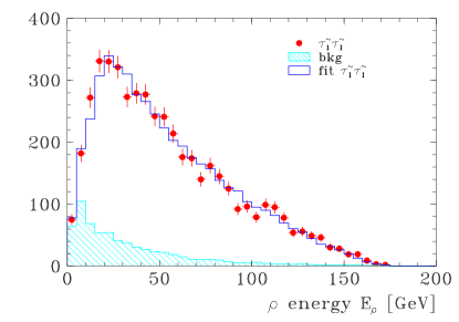
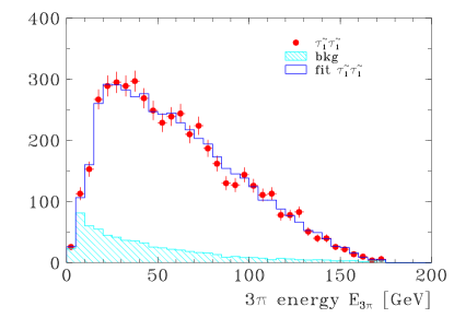
Figure 7: Hadron energy spectra of $\tau\to\rho\,\nu_{\tau}$ and $\tau\to 3\pi\,\nu_{\tau}$ decays from $e^{+}_{L}e^{-}_{R}\to{\tilde{\tau}}^{+}_{1}{\tilde{\tau}}^{-}_{1}$ production at $\sqrt{s}=500~{}\mathrm{GeV}$ with $P_{e^{-}}=+80\%$, $P_{e^{+}}=-60\%$ assuming ${\cal L}=250~{}\mathrm{fb}^{-1}$. The simulated data (dots) including SM and SUSY background (shaded histogram) are shown together with a fit to the ${\tilde{\tau}}_{1}$ mass.

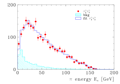
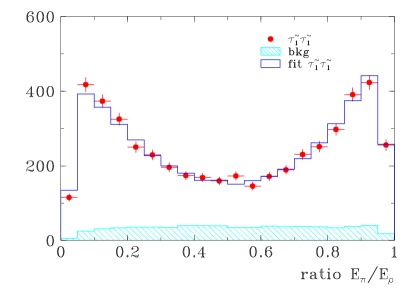
Figure 8: Pion energy spectrum of $\tau\to\pi\,\nu_{\tau}$ and ratio $E_{\pi}/E_{\rho}$ of $\tau\to\rho\,\nu_{\tau}\to\pi\pi^{0}\,\nu_{\tau}$ decays from $e^{+}_{L}e^{-}_{R}\to{\tilde{\tau}}^{+}_{1}{\tilde{\tau}}^{-}_{1}$ production at $\sqrt{s}=500~{}\mathrm{GeV}$ assuming ${\cal L}=250~{}\mathrm{fb}^{-1}$. The simulated data (dots) including SM and SUSY background (shaded histogram) are shown together with a fit to the $\tau$ polarisation ${\cal P}_{\tau}$ from ${\tilde{\tau}}_{1}$ decays.

Knowing the ${\tilde{\tau}}_{1}$ and $\tilde{\chi}^{0}_{1}$ masses, the $\pi$ energy spectrum and the decay characteristics of $\rho\to\pi\pi^{0}$ can be used to determine the $\tau$ polarisation. The energy distribution is harder for a $\pi$ emitted from a right-handed $\tau_{R}$ than from a left-handed $\tau_{L}$, as discussed above. The $E_{\pi}$ spectrum is shown in Fig. 8. A fit yields a $\tau$ polarisation of $P_{\tau}=0.860\pm 0.050$, consistent with the input value of $P_{\tau}^{th}=0.85$. Note that the residual background at low energies slightly reduces the sensitivity. In contrast to the $E_{\rho}$ distribution, there is a strong $P_{\tau}$ dependence on the $\rho$ polarisation, which can be measured through the decay $\rho\to\pi\pi^{0}$. Define the fraction of the energy carried by the charged $\pi$ as $z_{\pi}=E_{\pi}/E_{\rho}$. A right-handed $\tau_{R}$ prefers to decay into a longitudinally polarised $\rho_{L}$, and the $z_{\pi}$ distribution $\sim(2z_{\pi}-1)^{2}$ is peaked at $z_{\pi}\to 0$ and $1$, i.e. most of the energy is carried by one of the pions. A left-handed $\tau_{L}$ decays dominantly into a transversely polarised $\rho_{T}$, resulting in a $z_{\pi}$ distribution $\sim 2z_{\pi}\,(1-z_{\pi})$, i.e. a rather equal sharing of the energy between the two pions. The distribution of the ratio $E_{\pi}/E_{\rho}$ is shown in Fig. 8, with a flat contribution from the unpolarised background. From a fit to the $z_{\pi}$ distribution a value of $P_{\tau}=0.859\pm 0.045$ is obtained.

In summary. The simulation of the reaction $e^{+}_{L}e^{-}_{R}\to{\tilde{\tau}}^{+}_{1}{\tilde{\tau}}^{-}_{1}$ with ${\cal L}=250~{}\mathrm{fb}^{-1}$ at $\sqrt{s}=500~{}\mathrm{GeV}$ and beam polarisations of $P_{e^{-}}=+0.8$ and $P_{e^{+}}=-0.6$ demonstrates that the ${\tilde{\tau}}$ parameters can be determined with high precision. The cross section measurement appears feasible with an accuracy of $\delta\sigma/\sigma\simeq 3\,\%$, where the error is entirely due to systematics and is dominated by the uncertainty of the branching ratio. Using the information from all decay channels, the ${\tilde{\tau}}_{1}$ mass can be determined with an error of $\delta m_{{\tilde{\tau}}_{1}}=0.5~{}\mathrm{GeV}$ and the $\tau$ polarisation from ${\tilde{\tau}}_{1}$ decays can be measured with an accuracy of $\delta P_{\tau}=0.035$. As shown in Fig. 2, the cross section depends sensitively on the ${\tilde{\tau}}$ mixing angle. Applying eq. (18) and including the experimental resolutions, a value of $\cos 2\theta_{\tilde{\tau}}=-0.987\pm 0.02\,({\rm stat})\pm 0.06\,({\rm sys})$ can be derived for the ${\tilde{\tau}}$ mixing angle.

References

- [1] J. Wess and B. Zumino, Nucl. Phys. B 70 (1974) 39.
- [2] H. P. Nilles, Phys. Rept. 110 (1984) 1; H. E. Haber and G. L. Kane, Phys. Rep. 117 (1985) 75.
- [3] G. A. Blair, W. Porod and P. M. Zerwas, Phys. Rev. D 63 (2001) 017703 [hep-ph/0007107]; G. A. Blair, W. Porod and P. M. Zerwas, Eur. Phys. J. C in press [hep-ph/0210058].
- [4] E. Accomando et al. [ECFA/DESY LC Physics Working Group Collaboration], Phys. Rept. 299 (1998) 1 [hep-ph/9705442].
- [5] J. A. Aguilar-Saavedra et al., “TESLA Technical Design Report, Part III: Physics at an e+e- Linear Collider, Part IV: A Detector for TESLA”, DESY 2001-011 [hep-ph/0106315].
- [6] G. Moortgat-Pick et al., hep-ph/0210212; A. Freitas et al., hep-ph/0211108; P. M. Zerwas et al., hep-ph/0211076; to appear in the Proceedings of the 31st International Conference on High Energy Physics (ICHEP 2002), Amsterdam, 2002.
- [7] C. Blöchinger, H. Fraas, G. Moortgat-Pick and W. Porod, Eur. Phys. J. C 24 (2002) 297 [hep-ph/0201282]; S. Y. Choi, A. Djouadi, M. Guchait, J. Kalinowski, H. S. Song and P. M. Zerwas, Eur. Phys. J. C 14 (2000) 535 [hep-ph/0002033]. G. Moortgat-Pick, A. Bartl, H. Fraas and W. Majerotto, Eur. Phys. J. C 18 (2000) 379 [hep-ph/0007222]; J. L. Kneur and G. Moultaka, Phys. Rev. D 59 (1999) 015005 [hep-ph/9807336]; G. Moortgat-Pick and H. Fraas, Acta Phys. Polon. B 30 (1999) 1999 [hep-ph/9904209].
- [8] S. Y. Choi, J. Kalinowski, G. Moortgat-Pick and P. M. Zerwas, Eur. Phys. J. C 22 (2001) 563 [hep-ph/0108117]; S. Y. Choi, J. Kalinowski, G. Moortgat-Pick and P. M. Zerwas, Eur. Phys. J. C 22 (2001) 769 [hep-ph/0202039].
- [9] H. Baer, C. H. Chen, M. Drees, F. Paige and X. Tata, Phys. Rev. D 59 (1999) 055014 [hep-ph/9809223]; J. L. Feng and T. Moroi, Nucl. Phys. Proc. Suppl. 62 (1998) 108 [hep-ph/9707494]; V. D. Barger, T. Han and J. Jiang, Phys. Rev. D 63 (2001) 075002 [hep-ph/0006223]; J. F. Gunion, T. Han, J. Jiang and A. Sopczak, hep-ph/0212151.
- [10] E. Boos, G. Moortgat-Pick, H. U. Martyn, M. Sachwitz and A. Vologdin, hep-ph/0211040 and to appear in the Proceedings of the 10th International Conference on Supersymmetry and Unification of Fundamental Interactions, SUSY02, DESY, Hamburg 2002.
- [11] M. M. Nojiri, Phys. Rev. D 51 (1995) 6281 [hep-ph/9412374]; M. M. Nojiri, K. Fujii and T. Tsukamoto, Phys. Rev. D 54 (1996) 6756 [hep-ph/9606370].
- [12] B. C. Allanach et al., Eur. Phys. J.C 25 (2002) 113 [hep-ph/0202233]; N. Ghodbane and H.-U. Martyn, hep-ph/0201233.
- [13] S. Kraml, PhD Thesis, HEPHY Vienna, [hep-ph/9903257]; A. Bartl, H. Eberl, S. Kraml, W. Majerotto and W. Porod, Eur. Phys. J. directC 2 (2000); A. Bartl, K. Hidaka, T. Kernreiter and W. Porod, hep-ph/0207186; A. Bartl, K. Hidaka, T. Kernreiter and W. Porod, Phys. Lett. B 538 (2002) 137 [hep-ph/0204071]; M. Guchait and D. P. Roy, Phys. Lett. B 535 (2002) 243 [hep-ph/0205015].
- [14] A. Bartl, H. Fraas, W. Majerotto and N. Oshimo, Phys. Rev. D 40 (1989) 1594; G. Moortgat-Pick, A. Bartl, H. Fraas and W. Majerotto, LC-TH-2000-032, hep-ph/0002253.
- [15] G. Bélanger, F. Boudjema, A. Pukhov and A. Semenov, Comp. Phys. Comm. 149 (2002) 103.
- [16] A. Pukhov, E. Boos, M. Dubinin, V. Ilyin, D. Kovalenko, A. Kryukov, V. Savrin, S. Shichanin and A. Semenov, Report INP-MSU 98-41/542, hep-ph/9908288; A. Semenov, Comp. Phys. Comm. 115 (1998) 124 and hep-ph/0205020.
- [17] S. Jadach, Z. Was, R. Decker and J. H. Kühn, Comp. Phys. Comm. 76 (1993) 361.
- [18] M. Jezabek and J. H. Kühn, Nucl. Phys. B 320 (1989) 20; E. E. Boos and A. V. Sherstnev, Phys. Lett. B 534 (2002) 97 [hep-ph/0201271].
- [19] T. Sjöstrand et al., Comput. Phys. Commun. 135 (2001) 238 [hep-ph/0108264].
- [20] T. Ohl, Comput. Phys. Commun. 101 (1997) 269 [hep-ph/9607454].
- [21] M. Pohl and H. J. Schreiber, DESY-02-061 and hep-ex/0206009.