Abstract

We examine the effect of a more realistic Earth matter density model which takes into account of the local density variations along the baseline of a possible 2100 km very long baseline neutrino oscillation experiment. Its influence to the measurement of CP violation is investigated and a comparison with the commonly used global density models made. Significant differences are found in the comparison of the results of the different density models. PCAC 14.60.Pq , 11.30.Er

1 Introduction

The first results from KamLAND collaboration have recently been announced. The data demonstrate the disappearance of the reactor ${\bar{\nu}_{e}}$ at a high level of confidence [1] and hence corroborate the oscillation solution to the solar neutrino problem. Furthermore, the measurement excludes all but the Large Mixing Angle oscillation solutions (LMA) [2, 3]. In the fit of all solar neutrino data, prior the KamLAND result, including the neutral and charge currents, elastic scattering of both day and night data, the sign of the $\Delta{m}^{2}_{21}$ has been determined to be positive better than 3$\sigma$ for the solar mixing angle, $\theta_{\rm solar}<\pi/4$ [4, 5]. Among all the theoretical and phenomenological implications [6], the LMA solution establishes a favorable condition for a determination of the leptonic CP violation (CPV) phase [7] as a further probe of new physics in long baseline neutrino oscillation experiments [8].

Because of the smallness of the mixing angle $\theta_{13}$ [9], the signal of CPV effect will not be large in general. This makes the measurement of the CP phase a challenging task. Hence a detailed estimate of the various possible theoretical uncertainties and experimental errors will be crucial for the extraction of the CP phase. In particular, the matter effect has to be properly delineated in very long baseline (VLBL) oscillation experiments. The presently available Earth matter densities are modeled globally averaged values. They are given as functions that depend on the Earth radius only. However, Earth density is not a spherically symmetric function independent of the longitudinal and latitudinal coordinates. There are local density variations and can have abrupt density changes from place to place, radially or at different longitude and latitude. Although the average density model may be suitable for a variety of purposes, one wonders if it is adequate for an accurate extraction of the lepton CP phase by VLBL experiments. We can identify two specific questions which may affect the outcome of VLBL experiments and to which we have to look for answers: One question is how do we assign a realistic error to the model matter density? The other question is how do we estimate the effect of local matter density deviations from the available average? Unless we find satisfactory answers to these questions, we can not be sure that the errors in the extraction of the CP phase from VLBL is under control so that we can assign a good confidence level to the value of the CP phase obtained.

We have addressed the first question in a recent publication [10] where we proposed a set of density profiles which are randomly distributed around the average density to simulate the way that Earth matter density is determined. This approach provides a way to estimate the error, induced by the uncertainty of Earth matter density, on the CP phase determination. Other approaches have subsequently been proposed and a summary of several approaches can be found in [11].

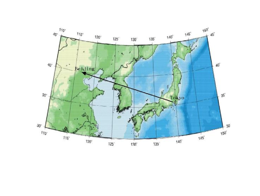
Figure 1: A schematic diagram of the H2B baseline which consists of a neutrino superbeam from J-PARC which is located about 60 km northeast of Tokyo, Japan to a detector near Beijing, China. The longitude and latitude of the neutrino source and target are indicated. The baseline is 2100 km.

In this paper we address the second question. We consider a more realistic matter density function along a specific baseline so that we can use a concrete example to examine the question. We will again focus on the recently approved high intensity proton synchrotron facility near Tokyo, Japan, i.e., the J-PARC (Japan Proton Accelerator Research Complex) [12]. We consider a VLBL, with $\nu_{\mu}$ and $\bar{\nu}_{\mu}$ beams from J-PARC to a detector located near Beijing, China, as depicted in Fig. 1. A preliminary study of the possibility of such a VLBL experiment, which we called H2B, can be found in Refs. [13] and [14]. In [13, 14] and subsequent studies a number of physics issues have been investigated: physics potentials of H2B, relevant backgrounds and errors [15], the effects of Earth matter density uncertainties [10], and the feasibility of measuring CP violation and atmospheric neutrino mass ordering in two joint LBL experiments [16]. Other studies on the matter effect on CP can be found in [17].

In Section 2 we discuss briefly the Earth density models and propose an alternative, more realistic density model for H2B. Section III presents a quick review of the approach of Ref. [10] for dealing with uncertainties of Earth matter density. Section IV discusses briefly the general statistical and other errors in CP measurements in LBL. A brief discussion is presented in Sec. V.

2 Earth density models and matter density distributions

In looking for the Earth matter effect, we are usually provided with some global model of Earth matter density, e.g., the PREM [18] or AK135 [19]. All presently available Earth density functions are not directly measured but obtained using a limited set of geophysics data which are analyzed by means of an inversion procedure. The density so obtained is a function of the depth from the Earth surface and any longitudinal and latitudinal variations are ignored. Consequently, in a given density model, the same density profile will be given for all baselines of the same length irrespective of their locality. All oscillation experiments of the same baselines length will have the same matter effect. Furthermore. since the matter density is a symmetric function along the baseline the matter effect will be the same when the neutrino beam source and detector sites are interchanged. Because of these simplified features, the existing density models are inherently of limited level of precision for VLBL. To improve the precision we have to know the specific density profile for a given VLBL. Or we have to establish the fact that the effect of the density variation is within the tolerance of the uncertainties that exist for the experiment.

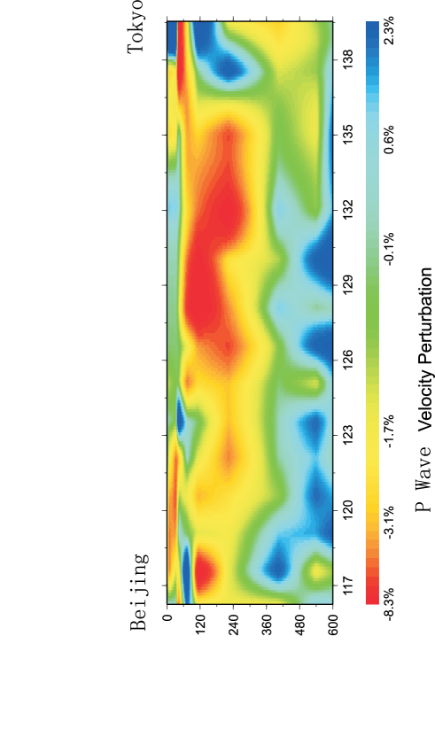
Figure 2: A 2-D plot of the earthquake P-wave data based on which the H2B-FTL density model is constructed. The scale from Tokyo to Beijing is the longitude in degrees and the scale perpendicular to it is the depth measured from Earth surface in units of km. The neutrino trajectory of H2B is a symmetric arc from Tokyo to Beijing, with its deepest penetration of Earth about 90 Km near 128^∘ longitude.

To demonstrate the effect of local density variations we make a detailed examination of the mass density profile along the baseline of H2B. Figure 2 shows the Earthquake P-wave velocity perturbation around the AK135. The color codes the size of the deviations from AK135. By mapping out the deviations along the baseline, we can obtain a more realistic density profile for H2B. We shall call this density profile for H2B the H2B-FTL density function. We will describe below how H2B-FTL is obtained. Three density profiles along the H2B baseline are shown in Fig. 3: PREM by the dotted curve, AK135 by the dashed curve, and H2B-FTL together with its typical error bars by the solid curve. The three density profiles provide a significant range of density variations which allow us to investigate the effect of Earth density on the determination of neutrino oscillation parameters in VLBL, in particular the CP phase.

Similar to PREM and AK135, H2B-FTL is based on the traveling time of earthquake waves. However, it is concentrated on the local region of the H2B baseline and therefore involves a much larger set of available data along the baseline than either PREM or AL135. Moreover, since it is a 3-dimensional density model, it contains significant information in the longitudinal and latitudinal directions, while PREM and AK135 are 1-dimension density models which provide information only along the radial direction. Hence H2B-FTL can better represent the actual density along the H2B path than either PREM or AK135.

The density function of H2B-FTL is related to that of AK135 via the following relation [20, 21],

$$\rho_{\rm H2B-FTL}=(1+\frac{1}{k}\frac{\delta v}{v})\rho_{\rm AK135},$$ (1)

where the AK135 density function, $\rho_{\rm AK135}$, can be found in [19]. $v$ is the P-wave velocity and $\delta v$ is the P-wave velocity correction to AK135 [22]. The geophysics consideration of the H2B path gives $k=0.2$. The ratio of the P-wave velocity correction to the P-wave velocity is the sole geophysics input in the corrections to AK135 and is given in terms of a large set of discrete data on the various positions along the baseline [20]. As shown in the scale at the bottom of Fig. 2, $\delta{v}/v$ varies from +2.3% to -8.3%.

As shown in Fig. 3, in several regions, H2B-FTL deviates from AK135 (PREM) beyond the usually cited allowed variation of $\pm 2\%$ ($\pm 5\%$). The strongest deviations can be recognized as the red and blue regions of Fig. 2. The red and blue regions represent respectively negative and positive corrections to AK135. As Fig. 1 displays, in its path from J-PARC to Beijing, a neutrino will go through the upper Earth mantle which exhibits plastic properties. It will first experience the Japan island crust (blue), the asthenosphere raised by Pacific slab in collision with the European-Asian slab (red), the normal asthenosphere under the Sea of Japan (red), the bottom of the West-CoSon-Man of west Korea peninsula (red), and the Bo Hai Sea of China (red). As shown in Fig. 3, global density models, such as PREM and AK135, can have significant deviations from the actual mass density profile of the H2B baseline.

The actual variance of the H2B-FTL is a complicate function along the baseline. For simplicity and to be conservative, we will ignore its position dependence and just take the maximal square root variance [20] to represent the density variance,

$$\sigma(\frac{\delta v}{v})=0.003$$ (2)

Then we have

$$\frac{\sigma(\rho_{\rm H2B-FTL})}{\rho_{\rm H2B-FTL}} = \frac{\rho_{\rm AK135}}{\rho_{\rm H2B-FTL}}\frac{1}{k}\sigma(\frac{\delta v}{v})$$ (3)

$$= 0.015\times\frac{\rho_{\rm AK135}}{\rho_{\rm H2B-FTL}}$$

which lies between $0.75\%$ and $3\%$. It should be mentioned that the H2B-FTL density profile consists of a huge data sample, hence the discretization size of the baseline in the path integral can be as small as 40 km, while the discretization size of PREM and AK135 along this baseline is 200 km. A smaller discretization size can reduce the error which is another factor that contributes to the higher level of precision of H2B-FTL.

3 Errors in CP violation measurements

We review briefly the method of [10] and define our notation. We are interested in quantifying the possible error caused by Earth density uncertainties. As usual, we define a CP-odd difference of neutrino oscillation probability functions,

$$D(\delta_{\rm CP},N_{e}(x)) \equiv P_{\alpha\beta}(\delta_{\rm CP},N_{e}(x))-P_{{\bar{\alpha}}{\bar{\beta}}}(\delta_{\rm CP},N_{\rm e}(x)),$$ (4)

where $\delta_{CP}$ is the CP phase, $N_{\rm e}(x)$ the electron density distribution function along the baseline $x$, and $P_{\alpha\beta}$ ($P_{\bar{\alpha}\bar{\beta}})$ the oscillation probability of $\nu_{\alpha}\rightarrow\nu_{\beta}$ ($\bar{\nu}_{\alpha}\rightarrow\bar{\nu}_{\beta}$). The electron density function $N_{\rm e}(x)$ is related to the Earth matter density $\rho(x)$ by the Avogadro number, $N_{\rm A}$, and the electron fraction, $Y_{\rm e}$, through the usual relationship, $N_{\rm e}(x)=N_{\rm A}Y_{\rm e}\rho(x)$. The dependence on the neutrino energy, mixture angles, and neutrino masses is suppressed.

We estimate the possible error from density uncertainty by following the formalism of  [10],

$$\delta D(\delta_{\rm CP},N_{\rm e}(x)) \equiv \sqrt{<{\left((P_{\alpha\beta}-P_{{\bar{\alpha}}{\bar{\beta}}})-<(P_{\alpha\beta}-P_{{\bar{\alpha}}{\bar{\beta}}})>\right)}^{2}>}$$ (5)

$$= \sqrt{\left(\delta(P_{\alpha\beta})\right)^{2}+\left(\delta(P_{{\bar{\alpha}}{\bar{\beta}}})\right)^{2}},$$

where $<\cdot\cdot\cdot>$ denotes a weighted average of a matter density dependent quantity. It is defined as a path integral of the quantity, along a given baseline, over an ensemble of possible variations of Earth matter density profiles, $N_{\rm e}(x)$, weighted by a logarithmic normal distribution functional $F[N_{e}(x)]$ for non-negative quantities [10], e.g.,

$$<P_{\alpha\beta}> \equiv \int[{\cal D}N_{\rm e}(x)]F[N_{\rm e}(x)]P_{\alpha\beta}(\delta_{CP},N_{\rm e}(x)).$$ (6)

Therefore we interpret the average matter density $\hat{N}_{\rm e}(x)$, such as PREM and AK135, as a weighted average over all samples of possible density profiles,

$$\hat{N}_{\rm e}(x) \equiv <N_{\rm e}(x)>=\int[{\cal D}N_{\rm e}(x)]F[N_{\rm e}(x)]N_{\rm e}(x).$$ (7)

The matter density uncertainty is given as usual by

$$\sigma(x) \equiv \sqrt{<N^{2}_{\rm e}(x)>-\left(\hat{N}_{\rm e}(x)\right)^{2}}$$ (8)

The level of precision of a density model with a given $\hat{N}(x)$ and $\sigma(x)$ can be measured by

$$r(x) \equiv \frac{\sigma(x)}{{\hat{N}}_{\rm e}(x)}.$$ (9)

To do the functional integral, the integration path along the neutrino baseline is discretized according to the available geophysical information. For the H2B baseline, the discretization size for H2B-FTL is 40 km, which is much smaller than the 200 km discretization size suitable for PREM or AK135. The smaller discretization size is helpful in reducing the errors in the functional integration.

We remark that an alternative parameterization of the Earth matter density uncertainty is to give the average matter density a fixed deviation, i.e., taking the density function to be $N^{\prime}(x)=(1\pm r^{\prime}(x))\hat{N}(x)$, where $r^{\prime}(x)$ is the density uncertainty. Conventionally, $\hat{N}(x)$ is given by PREM or AK135 and $r^{\prime}(x)$ is respectively 0.05 or 0.02. As discussed in [10], this parameterization will lead to a larger uncertainty in the extraction of the CP phase than the present approach.

The above formulation can be readily adopted to the measurable quantity of the event number. Unless noted otherwise in the calculation of event number, we assume 6500 interacting muon neutrinos for H2B.

For the numerical calculation, we adopted the following values for the solar and atmospherical neutrino mass square differences and the corresponding mixing angles:

$$\Delta m^{2}_{\rm solar} = 5.0\times{10}^{-5}~{}{\rm eV^{2}},\hskip 8.61108pt\tan^{2}\theta_{12}~{}=~{}0.42,$$

$$\Delta m^{2}_{\rm atm} = 3.0\times{10}^{-3}~{}{\rm eV^{2}},\hskip 8.61108pt\sin^{2}2\theta_{23}~{}=~{}0.99.$$ (10)

Since the CPV effect is proportional to $\theta_{13}$, a larger value of $\sin^{2}2\theta_{13}$ will be more favorable for its measurement. The CHOOZ bound is $\sin^{2}2\theta_{13}\leq 0.15$ [9]. In Fig. 4 we plot the CPV event number vs the CP phase. We show several different values of $\sin^{2}2\theta_{13}$ and the beam energies. One can see from the upper panel Fig. 4 that, for this number of testing muons there will be little sensitivity in the CP phase measurement in H2B if $\sin^{2}2\theta_{13}<0.01$. However with a higher number of testing muons the sensitivity can be increased. In the following calculation we will use $\sin^{2}2\theta_{13}=0.08$ for illustration. However, for comparison, we will also show some results for $\sin^{2}2\theta_{13}=0.01$.

To select the appropriate neutrino energy, we have examined the oscillation probabilities of 1.5, 4, 4.5, 5, and 8 GeV. As shown in the lower panel of Fig. 4, $4.5$ GeV is the optimal energy which will be used in all subsequent calculations. It should be noted that Fig. 4 employs the density distribution H2B-FTL, but different density model does not change the optimal energy and the sensitivity in $\theta_{13}$.

To examine the difference among the different density models we define the following quantity which provides a gross measurement of the ”pure” CP effect,

$$\Delta{D}(\delta_{\rm CP})\equiv D(\delta_{CP},N_{\rm e}(x))-D(\delta_{CP}=0,N_{\rm e}(x)).$$ (11)

Then we can define a quantitative measure of the significance of the CPV signal by the ratio of the ”pure” CPV effect and the corresponding quantity which also contains the matter effect,

$$S_{\rm den}(\delta_{\rm CP})\equiv\frac{\Delta D(\delta_{\rm CP})}{\delta D(\delta_{\rm CP},N_{\rm e}(x))}$$ (12)

A larger $S_{\rm den}(\delta_{\rm CP})$ gives a stronger CP signal relative to the matter effect, we require that $S_{\rm den}(\delta_{\rm CP})$ be significantly greater than 1. In Fig. 5, we plot $S_{\rm den}(\delta_{\rm CP})$ against the CP phase $\delta_{\rm CP}$. Indeed H2B-FTL gives a signal better than AK135 and PREM for $\delta_{CP}$ away from 0 and $\pi$ where the CPV effect vanishes.

To compare the H2B-FTL with other density model, e.g., the AK135, we define

$$\tilde{\delta}D(\delta_{CP}) = D(\delta_{\rm CP},N_{\rm e}(x))_{({\rm H2B-FTL})}-D(\delta_{\rm CP},N_{\rm e}(x))_{({\rm AK135})}.$$ (13)

We can define a significance measure of the CPV effect with the difference of density models,

$$\tilde{S}_{\rm den}(\delta_{\rm CP}) = \frac{\Delta D(\delta_{\rm CP})}{\tilde{\delta}{D}(\delta_{\rm CP})}.$$ (14)

We plot $\tilde{S}_{\rm den}(\delta_{\rm C})$ in Fig. 6. We see that the difference in density models is always larger than the CP difference. This again underlines the fact that a realistic density is necessary.

In Fig. 7 we plot the ”pure” CP effect, $\Delta D(\delta_{\rm CP})$ given in Eq. (11), as a function of the CP phase for the three density models together with the error bars for H2B-FTL. In general, AK135 is 3$\sigma$ away and PREM is 6$\sigma$ away from H2B-FTL for a given CP phase, indicating significant differences between the different density models.

4 Statistical and other Errors in CPV measurements

In this section we present the result of our study of the statistical errors, the background effects, and the systematic uncertainties, and contrast them with the effect of density uncertainties. Our treatment of statistical errors, background effects, and systematic uncertainties follows that of Ref. [15]. They are represented by their respective error factors denoted as $f$ (statistical), $r$ (background), and $g$ (systematic). Denoting the variance of their combined effect by $\sigma_{\rm SBS}$, we can define the significance of measure of the CPV effect with respect to this combined variance,

$$S_{\rm SBS} \equiv \frac{\Delta D(\delta_{\rm CP})}{\sigma_{\rm SBS}}$$ (15)

Obviously $S_{\rm SBS}$ is only meaningful for the case of a sufficiently large number of interacting $\nu_{\mu}$’s. For the numerical calculation we take the statistical factor $f=0.02$, the background factor $r=0.01$, and the systematic factor $g=0$ as used in [16]. We show in the upper left corner of Fig. 7 a representative error bar for this combined error.

In Fig. 8 we plot both $S_{\rm SBS}$, Eq. (15), and $\tilde{S}_{\rm den}$, Eq. (14), for $\sin^{2}2\theta_{13}=0.08$ and 0.01 and for two total number of interacting $\nu_{\mu}$’s, 6500 and 650. We see that for several hundred interacting $\nu_{\mu}$’s, no CPV effect is expected to be measurable. For several thousands of $\nu_{\mu}$ muons, we have a chance to observe the CPV effect. With the CPV variable we consider here Earth matter uncertainty can be ignored safely if H2B-FTL model is employed, but the significance will be worse if other density model ($\tilde{S}_{\rm den}$) is adopted.

5 Discussions

In this paper we investigated the potential error caused by the uncertainties of earth matter density. We also consider the other errors, such as the statistical error, in the context of intended H2B physics. We found that the more realistic density model, H2B-FTL, the matter density variation induces a rather small error which allows a meaningful separation of H2B-FTL from AK135 and PREM. With CPV variable we used, i.e., the CP difference, the statistical and other errors generally dominate over the difference of the density models. Therefore, a different approach of the CP measurement, such as that used in [16] has to be investigated.

Figure 3: The vertical axis is the Earth effective matter density profile, where $Y_{\rm e}\rho(x)$, $Y_{\rm e}=0.494$ is the electron fraction and $\rho(x)$ is the matter density in gram/cm³. The horizontal axis is the baseline from J-PARC (0 km) to Beijing (2100 km) in km. The PREM and AK135 are world average densities and H2B-FTL is constructed specifically for H2B. The error bars on the solid curve are the uncertainties of H2B-FTL defined in Eq. (3). Note that the densities have been scaled by a factor of the nuclear composition, $Y_{\rm e}=Z/A\sim 0.494$, which is suitable in the region of H2B.

Figure 4: The $\nu_{\rm e}$ and $\bar{\nu}_{\rm e}$ number difference, corresponding to Eq. (4) with 6500 interacting $\nu_{\mu}$, vs the leptonic CP phase. The curves in the upper panel are for different values of $\sin^{2}2\theta_{13}$ and those in the lower panel are for different energies. The horizontal axis which is the CP phase $\delta_{\rm CP}$ is in units of $2\pi$

Figure 5: The CPV signal significance $S_{\rm den}$, Eq. (12), vs the CP phase. The solid line is for H2B-FTL with a $3\%$ uncertainty, the short-dashed line is for AK135, and the dashed line for PREM. The upper panel has $\sin^{2}2\theta_{13}=0.01$ and the lower panel $\sin^{2}2\theta_{13}=0.08$. The scale of the horizontal axis is in units of 2$\pi$.

Figure 6: The CPV signal significance $\tilde{S}_{\rm den}$, Eq. (14), vs the CP phase. The solid curves is for $\sin^{2}2\theta_{13}=0.01$ and dashed curve for $\sin^{2}2\theta_{13}=0.08$. The horizontal axis is in units of 2$\pi$.

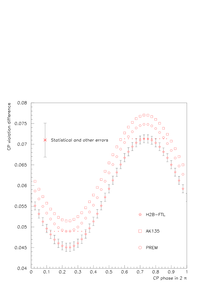
Figure 7: The CPV difference $\delta D(\delta_{\rm CP})$, Eq. (5), vs the CP phase for $\sin^{2}2\theta_{13}=0.08$. The squares are for AK135, the circles for PREM, and the stars for H2B-FTL. The error bars associated with the stars are for H1B-FTL. A typical size of the statistical plus background errors is shown in the upper left corner. See the relevant discussion in Sec. 4.

Figure 8: The CPV signal significance vs the CP phase. The solid line is for $\tilde{S}_{\rm den}$, Eq. (14). The dashed lines are for the signal significance $S_{\rm SBS}$, Eq. (15). The thin dashed line has 650 interacting $\nu_{\mu}$ and the heavy dashed line has 6500 interacting $\nu_{\mu}$. The upper panel is for $\sin^{2}2\theta_{13}=0.01$ while the lower panel for $\sin^{2}2\theta_{13}=0.08$

References

- [1] KamLAND Collab., K. Eguchi et al., Phys. Rev. Lett. 90, 021802 (2003) (arXiv: hep-ex/0212021).
- [2] SNO Collab., Q.R. Ahmad et al., Phys. Rev. Lett. 87, 071301 (2001) (arXiv: nucl-ex/0106015); Phys. Rev. Lett. 89, 011302 (2002) (arXiv: nucl-ex/0204009).
- [3] J.N. Bahcall, M.C. Gonzalez-Garcia, and Carlos Pena-Garay, JHEP 0207:054 (2002) (arXiv: hep-ph/0204314)
- [4] V. Barger, D. Marfatia, K. Whisnant and B.P Wood, Phys. Lett. B573 (2002) 179.
- [5] J.N. Bahcall, M.C. Gonzalez-Garcia, and Carlos Peã-Garay, Solar Neutrinos before and after KamLAND, arXiv: hep-ph/0212147.
- [6] C. D. Froggatt, H. B. Nielsen, and Y. Takanishi, Nucl. Phys., B631 285-306 (2002) (arXiv: hep-ph/0201152); O. L. G. Peres and A. Yu. Smirnov, Nucl. Phys. Proc. Suppl. 110 355 (2002) (arXiv: hep-ph/0201069); Xiao-Jun Bi and Yuan-Ben Dai, arXiv: hep-ph/0204317; S. Antusch, J. Kersten, M. Lindner, and M. Ratz, Phys. Lett. B544, 1 (2002) (arXiv: hep-ph/0206078); Zhi-zhong Xing, Phys. Lett. B550, 178 (2002) (arXiv: hep-ph/02102776).
- [7] T. Endoh, S. Kaneko, S.K. Kang, T. Morozumi, and M. Tanimoto, Phys. Rev. Lett., 89 231601 (2002) (arXiv: hep-ph/0209020); John Ellis and Martti Raidal, Nucl. Phys. B643, 229 (2002) (arXiv: hep-ph/0206174); Y. Farzan and A. Yu. Smirnov, Phys. Rev., D65, 113001 (2002) (arXiv: hep-ph/0201195); M. C. Gonzalez-Garcia, Y. Grossman, A. Gusso, and Y. Nir, Phys. Rev. D64 096006 (2001) (arXiv: hep-ph/0105159); J. Burguet-Castell, M.B. Gavela, J.J. Gomez-Cadenas, P. Hernandez, and O. Mena, Nucl. Phys. B608, 301 (2001) (arXiv: hep-ph/0103258); S. Pastor, J. Segura, V.B. Semikoz, and J.W.F. Valle, Nucl. Phys. B566, 92 (2000) (arXiv: hep-ph/9905405). K. Dick, M. Freund, M. Lindner, and A. Romanino, Nucl. Phys., B562, 29 (1999) (arXiv: hep-ph/9903308).
- [8] BNL Neutrino Working Group:hep-ex/0211001; J. Burguet-Castell, M.B. Gavela, J.J. Gomez-Cadenas, P. Hernandez, and O. Mena, Nucl. Phys., B646, 301 (2002) (arXiv: hep-ph/0207080); Y. F. Wang, K. Whisnant, Zhaohua Xiong, Jin Min Yang, and Bing-Lin Young, Phys. Rev., D65 (2002) (2002) (arXiv: 0111317); K. Dick, Martin Freund, Patrick Huber, and Manfred Lindner, Nucl. Phys. B598, 543 (2001) (arXiv: hep-ph/0008016); V. Barger, S. Geer, R. Raja, and K. Whisnant, Phys. Rev. D62 013004 (2000) (arXiv: hep-ph/9911524)
- [9] CHOOZ Collaboration, M. Apllonio et al., Phys. Lett., B466, 415 (1999) (arXiv: hep-ex/9907037).
- [10] Lian-You Shan, Bing-Lin Yong, and Xinmin Zhang, Phys. Rev., D66 053012 (2002) (arXiv: hep-ph/0110414).
- [11] B. Jacobsson, T. Ohlsson, H. Snellman, and W. Winter, Phys. Lett., B532, 259 (2002) (arXiv: hep-ph/0112138); B. Jacobsson, T. Ohlsson, H. Snellman, and W. Winter, talk given at NuFact ’02, London, arXiv: hep-ph/0209147.
- [12] For a description of J-PARC, we refer to its website http://jkj.tokai.jaeri.go.jp/. Previously the facility has been referred to by the acronym JHF or HIPA.
- [13] H.S. Chen, et al., Report of a Study on H2B, Prospect of a very long baseline neutrino oscillation experiment HIPA to Beijing, VLBL Study Group-H2B-1, IHEP-EP-2001-01, May 29, 2001, arXiv: hep-hp/0104266
- [14] M. Aoki, K. Hagiwara, Y. Hayato, T. Kobayashi, T. Nakaya, K. Nishikawa (Kyoto U.), N. Okamura, ”Prospects of very long baseline neutrino oscillation experiments with the KEK/JAERI high intensity proton accelerator”, KEK-TH-798, VPI-IPPAP-01-03, Dec 2001, arXiv: hep-ph/0112338; and talk given at the 4th International Conference on B Physics and CP Violation (BCP 4), Ago Town, Mie Prefecture, Japan, 19-23 Feb 2001, arXiv: hep-ph/0104220.
- [15] Yi-Fang Wang, K. Whisnant, and Bing-Lin Young, Phys. Rev., D65 073006 (2002) (arXiv: hep-ph/0109053).
- [16] K. Whisnant, Jin Min Yang, and Bing-Lin Young, Phys. Rev. D67 (2003) 013004 (arXiv: hep-ph/0208193).
- [17] H. Yokomakura, K. Kimura, and A. Takamura, Phys. Lett. B544, 286 (2002) (arXiv: hep-ph/0207174); T. Hattori, Tsutom Hasuike, and Seiichi Wakaizumi, Phys. Rev., D65 073027 (2002) (hep-ph/0109124); T. Ohlsson and H. Snellman, Eur. Phys. J. C20, 507 (2001) (arXiv: hep-ph/0103252).
- [18] A.M. Dziewonsky and D.L. Andson, Phys. Earth Planet Int., 25, 507 (1981).
- [19] B.L.N. Kennet et al., Geophys. J. Int., 122, 108 (1995); J.P. Montagner et. al., Geophys. J. Int., 125, 229 (1995).
- [20] Fu-Tian Liu et al., Three-dimensional seismic tomography of oceanic lithosphere, Project 863 Study report, ( 863-820-01-04 ); Fu-Tian Liu et al., Geophys. J. Int., 101, 379 (1990).
- [21] K.E. Bullen, The Earth’s density, Chapman and Hall , London (1975).
- [22] F.T. Liu and A. Jin, Seismic Tomography of China, in Seismic Tomography: Theory and Practice, Ed. by H.M. Iyer and K. Hiahara, Chapman and Hall , London (1993).