DESY 02-229 hep-ph/0302272 Nucl. Phys. B 661 (2003) 62-82.
Proton Decay in a Consistent Supersymmetric SU(5) GUT Model
line

Abstract

It is widely believed that minimal supersymmetric SU(5) GUTs have been excluded by the SuperKamiokande bound for the proton decay rate. In the minimal model, however, the theoretical prediction assumes unification of Yukawa couplings, $Y_{d}=Y_{e}$, which is known to be badly violated. We analyze the implications of this fact for the proton decay rate. In a consistent SU(5) model with higher dimensional operators, where SU(5) relations among Yukawa couplings hold, the proton decay rate can be several orders of magnitude smaller than the present experimental bound.

PACS numbers: 11.10.Hi, 12.10.Dm, 12.60.Jv, 13.30.-a, 14.20.Dh

1 Introduction

Supersymmetric Grand Unified Theories (SUSY GUTs) [1] provide a beautiful framework for theories beyond the standard model (SM) of particle physics. They combine several attractive ideas, namely supersymmetry and unification of matter and interactions. A crucial prediction of SUSY GUTs is the instability of the proton [2], and the long-lasting search for proton decay has put a strong constraint on unified theories.

The simplest models are based on the gauge group SU(5). The SM particles can be grouped into two multiplets per generation, no additional matter particles are needed. Hereby, the down quark and charged lepton Yukawa couplings are unified. The GUT scale is set by the unification of the gauge couplings around $2\times 10^{16}$ GeV in the Minimal Supersymmetric Standard Model (MSSM).

SU(5) based models have been studied in great detail. Recently the simplest version, minimal supersymmetric SU(5) [1], was claimed to be excluded due to the SuperKamiokande bound on proton decay [3, 4]. The exclusion of the “prototype” GUT model is an important result and it is worth analyzing the underlying assumptions carefully.

One ingredient is the sfermion mixings [5] which are essentially unknown and which are neglected in refs. [3, 4]. Taking these mixings into account one can suppress the proton decay rate below the experimental bound [5, 6]. Another important question concerns the failure of down quark and charged lepton Yukawa couplings to unify. To our knowledge, all previous analyses assumed exact unification at the GUT scale, $Y_{d}=Y_{e}$, and then used the down quark matrix to study proton decay. The decay width, however, is strongly dependent on flavour mixing and there is no reason not to take, for instance, the lepton matrix instead.

The failure of Yukawa unification can be accounted for by adding operators induced by Planck scale effects [6]. Since the GUT scale is only about two orders below the Planck scale, differences between down quarks and charged leptons can be explained by such operators. In addition, they also affect the proton decay operators.

In this paper, we start with minimal supersymmetric SU(5) and discuss the influence of flavour mixing on proton decay. After that, we will study the impact of higher dimensional operators on proton decay. In particular, we consider two simple models where the decay rate is well below the experimental limit.

The outline of the paper is as follows: After briefly describing the supersymmetric SU(5) GUT model (Section 2) and analyzing the dimension five operators (Section 3), we discuss the results of the different scenarios in Section 4. Important and clarifying details are given in the Appendices.

2 Supersymmetric SU(5) GUTs

We start this section by briefly describing the minimal supersymmetric SU(5) GUT model [1]. It contains three generations of chiral matter multiplets,

$$\mathsf{10}_{j} =(Q,u^{\text{\sc c}},e^{\text{\sc c}})_{j}\ ,$$

$$\mathsf{5}^{*}_{j} =(d^{\text{\sc c}},L)_{j}\ ,$$

and a vector multiplet $A(\mathsf{24})$ which includes the twelve gauge bosons of the SM and twelve additional ones, the $X$ and $Y$ bosons. Because of their electric and colour charges, the latter mediate proton decay via $d=6$ operators. At the GUT scale, SU(5) is broken to ${\sf G_{SM}=SU(3)\times SU(2)\times U(1)_{Y}}$ by an adjoint Higgs multiplet $\Sigma(\mathsf{24})$. A pair of quintets, $H(\mathsf{5})$ and $\overline{H}(\mathsf{5}^{*})$, then breaks ${\sf G_{SM}}$ to ${\sf SU(3)\times U(1)_{\text{em}}}$ at the electroweak scale. The superpotential is given by

$$\begin{split}W&=\tfrac{1}{2}m\operatorname{tr}\Sigma^{2}+\tfrac{1}{3}a\operatorname{tr}\Sigma^{3}+\lambda\overline{H}(\mathsf{5}^{*})\,(\Sigma+3\sigma)\,H(\mathsf{5})\\ &\quad+\tfrac{1}{4}\,Y_{1}^{ij}\,\mathsf{10}_{i}\;\mathsf{10}_{j}\;H(\mathsf{5})+\sqrt{2}\,Y_{2}^{ij}\,\mathsf{10}_{i}\;\mathsf{5}^{*}_{j}\;\overline{H}(\mathsf{5}^{*})\ .\end{split}$$ (1)

The adjoint Higgs multiplet,

$$\Sigma(\mathsf{24})=\left(\begin{array}[]{cc}\Sigma_{8}&\Sigma_{(3,2)}\\ \Sigma_{(3^{*},2)}&\Sigma_{3}\end{array}\right)+\frac{1}{2\sqrt{15}}\left(\begin{array}[]{cc}2&0\\ 0&-3\end{array}\right)\Sigma_{24}\ ,$$

acquires the vacuum expectation value (VEV)

$$\left\langle\Sigma\right\rangle=\sigma\operatorname{diag}(2,2,2,-3,-3)\ ,$$

so that the X and Y bosons become massive,

$$M_{V}\equiv M_{X}=M_{Y}=5\sqrt{2}g_{5}\sigma\ ,$$ (2)

whereas the SM particles remain massless. Here $g_{5}$ is the SU(5) gauge coupling. The components $\Sigma_{8}$ and $\Sigma_{3}$ of $\Sigma(\mathsf{24})$ both acquire the mass

$$M_{\Sigma}\equiv M_{8}=M_{3}=\tfrac{5}{2}m\ ,$$

while $\Sigma_{(3,2)}$ and $\Sigma_{(3^{*},2)}$ form vector multiplets of mass $M_{V}$ together with the gauge multiplets. Finally, the mass of the singlet component $\Sigma_{24}$ is $\tfrac{1}{2}m$.

The pair of quintets, $H(\mathsf{5})$ and $\overline{H}(\mathsf{5}^{*})$, contains the SM Higgs doublets, $H_{f}$ and $\overline{H}_{f}$, which break $\mathsf{G_{SM}}$, and colour triplets, $H_{\text{\sc c}}$ and $\overline{H}_{\text{\sc c}}$, respectively. To have massless Higgs doublets $H_{f}$ and $\overline{H}_{f}$, while their colour-triplet partners (leptoquarks) are kept super-heavy,

$$M_{H_{\text{\sc c}}}=M_{\overline{H}_{\text{\sc c}}}=5\lambda\sigma\ ,$$ (3)

the mass parameters of $H(\mathsf{5})$ and $\overline{H}(\mathsf{5}^{*})$ have to be fine-tuned ${\cal O}(\frac{v}{\sigma})\sim 10^{-13}$. This is the so-called doublet-triplet-splitting problem. As we will see below, RGE analysis gives constraints on the masses of the new particles.

Expressed in terms of SM superfields, the Yukawa interactions are

$$\begin{split}W_{Y}=\;&Y_{u}^{ij}\,Q_{i}\,u^{\text{\sc c}}_{j}\,H_{f}+Y_{d}^{ij}\,Q_{i}\,d_{j}^{\text{\sc c}}\,\overline{H}_{f}+Y_{e}^{ij}\,e_{i}^{\text{\sc c}}\,L_{j}\,\overline{H}_{f}\\ &+\tfrac{1}{2}Y_{qq}^{ij}\,Q_{i}\,Q_{j}\,H_{\text{\sc c}}+Y_{ql}^{ij}\,Q_{i}\,L_{j}\,\overline{H}_{\text{\sc c}}+Y_{ue}^{ij}\,u_{i}^{\text{\sc c}}\,e^{\text{\sc c}}_{j}\,H_{\text{\sc c}}+Y_{ud}^{ij}\,u_{i}^{\text{\sc c}}\,d_{j}^{\text{\sc c}}\,\overline{H}_{\text{\sc c}}\ ,\end{split}$$ (4)

where

$$Y_{u}=Y_{qq}=Y_{ue}=Y_{1}\ ,$$ (5)

$$Y_{d}=Y_{e}=Y_{ql}=Y_{ud}=Y_{2}\ .$$ (6)

In particular the Yukawa couplings of down quarks and charged leptons are unified. While $m_{b}=m_{\tau}$ can be fulfilled at the GUT scale, it fails for the first and second generation. This problem can be solved by adding higher dimensional operators due to physics at the Planck scale so that [6]

$$W_{\Sigma}=\tfrac{1}{2}m\operatorname{tr}\Sigma^{2}+\tfrac{1}{3}a\operatorname{tr}\Sigma^{3}+b\frac{(\operatorname{tr}\Sigma^{2})^{2}}{M_{\text{Pl}}}+c\frac{\operatorname{tr}\Sigma^{4}}{M_{\text{Pl}}}\ .$$ (7)

Now the masses of $\Sigma_{3}$ and $\Sigma_{8}$ are no longer identical, which will affect the constraints on the leptoquark mass. Including possible couplings up to order $1/M_{\text{Pl}}$, the Yukawa interactions read

$$\begin{split}W_{Y}&=\frac{1}{4}\,\epsilon_{abcde}\left(Y_{1}^{ij}\,\mathsf{10}_{i}^{ab}\,\mathsf{10}_{j}^{cd}\,H^{e}+f_{1}^{ij}\,\mathsf{10}_{i}^{ab}\,\mathsf{10}_{j}^{cd}\,\frac{\Sigma^{e}_{f}}{M_{\text{Pl}}}\,H^{f}+f_{2}^{ij}\,\mathsf{10}_{i}^{ab}\,\mathsf{10}_{j}^{cf}\,H^{d}\,\frac{\Sigma^{e}_{f}}{M_{\text{Pl}}}\right)\\ &\quad+\sqrt{2}\left(Y_{2}^{ij}\,\overline{H}_{a}\,\mathsf{10}_{i}^{ab}\,\mathsf{5}^{*}_{jb}+h_{1}^{ij}\,\overline{H}_{a}\,\frac{\Sigma^{a}_{b}}{M_{\text{Pl}}}\,\mathsf{10}_{i}^{bc}\,\mathsf{5}^{*}_{jc}+h_{2}^{ij}\,\overline{H}_{a}\,\mathsf{10}_{i}^{ab}\,\frac{\Sigma_{b}^{c}}{M_{\text{Pl}}}\,\mathsf{5}^{*}_{jc}\right)\ .\end{split}$$ (8)

Then the Yukawa couplings are given by

$$\begin{split}Y_{u}&=Y_{1}+3\frac{\sigma}{M_{\text{Pl}}}f_{1}^{S}+\frac{1}{4}\frac{\sigma}{M_{\text{Pl}}}\left(3f_{2}^{S}+5f_{2}^{A}\right)\ ,\\ Y_{d}&=Y_{2}-3\frac{\sigma}{M_{\text{Pl}}}h_{1}+2\frac{\sigma}{M_{\text{Pl}}}h_{2}\ ,\\ Y_{e}&=Y_{2}-3\frac{\sigma}{M_{\text{Pl}}}h_{1}-3\frac{\sigma}{M_{\text{Pl}}}h_{2}\ .\end{split}$$ (9)

Here $\sigma/M_{\text{Pl}}\sim{\cal O}(10^{-2})$, and $S$ and $A$ denote the symmetric and antisymmetric parts of the matrices, respectively. Thus the three Yukawa matrices, which are related to masses and mixing angles at $M_{Z}$ by the RGEs, are determined by six matrices.

From eqn. (9) one reads off,

$$Y_{d}-Y_{e}=5\frac{\sigma}{M_{\text{Pl}}}h_{2}\ .$$ (10)

Hence the failure of Yukawa unification is naturally accounted for by the presence of $h_{2}$. Note that we do not need to introduce any additional field at $M_{\text{GUT}}$ to obtain this relation; it just arises from corrections ${\cal O}(\sigma/M_{\text{Pl}})$. Therefore we call this model a consistent supersymmetric SU(5) GUT model. In the minimal model, $Y_{qq}=Y_{ue}=Y_{u}$; furthermore, one usually chooses $Y_{ql}=Y_{ud}=Y_{d}$. Note, however, that the choices $Y_{ql}=Y_{ud}=Y_{e}$ or $Y_{ql}=Y_{d}$, $Y_{ud}=Y_{e}$ would be equally justified. As we shall see, this ambiguity strongly affects the proton decay rate.

Finally, in general right-handed neutrinos can be added as singlets in SU(5) models. With ${\mathsf{1}}_{j}=\nu^{\text{\sc c}}_{j}$, the Yukawa interactions read

$$W_{Y}^{\nu}=Y_{\text{\sc d}}^{ij}\,\mathsf{1}_{i}\;\mathsf{5}^{*}_{j}\;H(\mathsf{5})+M^{ij}\,\mathsf{1}_{i}\;\mathsf{1}_{j}\ ,$$

where $M$ is the Majorana mass matrix with eigenvalues ${\cal O}(M_{\text{GUT}})$.

3 Analysis of dimension five operators

The evolution of the proton decay rate based on dimension five operators involves a number of parameters and assumptions which have changed in analyses during the past years. In this section we therefore list the main ingredients of our quantitative analysis. Technical details are given the Appendices.

Figure 1: Proton Decay via dimension five operators: They result from exchange of the leptoquarks followed by gaugino or higgsino dressing.

Integrating out the leptoquarks in eqn. (4), two dimension five operators remain which lead to proton decay (fig. 1) [7],

$$W_{5}=\frac{1}{M_{H_{\text{\sc c}}}}\left[\,\frac{1}{2}\,Y_{qq}^{ij}\,Y_{ql}^{km}\,\left(Q_{i}\,Q_{j}\right)\left(Q_{k}\,L_{m}\right)+Y_{ue}^{ij}\,Y_{ud}^{km}\,\left(u_{i}^{\text{\sc c}}\,e_{j}^{\text{\sc c}}\right)\left(u_{k}^{\text{\sc c}}\,d_{m}^{\text{\sc c}}\right)\,\right]\ ,$$ (11)

called the $LLLL$ and $RRRR$ operator, respectively. The scalars are transformed to their fermionic partners by exchange of a gauge or Higgs fermion. Neglecting external momenta, the triangle diagram factor reads, up to a coefficient ${\cal K}$ depending on the exchange particle,

$$\int\frac{d^{4}k}{i(2\pi)^{4}}\,\frac{1}{m_{1}^{2}-k^{2}}\,\frac{1}{m_{2}^{2}-k^{2}}\,\frac{1}{M-\hbox to0.0pt{\hbox{$\mskip 1.0mu/$}\hss}k}=\frac{1}{(4\pi)^{2}}f(M;m_{1},m_{2})\ ,$$ (12)

with

$$f(M;m_{1},m_{2})=\frac{M}{m_{1}^{2}-m_{2}^{2}}\left(\frac{m_{1}^{2}}{m_{1}^{2}-M^{2}}\,\ln\frac{m_{1}^{2}}{M^{2}}-\frac{m_{2}^{2}}{m_{2}^{2}-M^{2}}\,\ln\frac{m_{2}^{2}}{M^{2}}\right)\ ,$$ (13)

where $M$ and $m_{j}$ denote the gaugino and sfermion masses, respectively.

As a result of Bose statistics for superfields, the total anti-symmetry in the colour index requires that these operators are flavour non-diagonal [8]. The dominant decay mode is therefore $p\to K\bar{\nu}$. Since the dressing with gluinos and neutralinos is flavour diagonal, the chargino exchange diagrams are dominant [9, 10]. The wino exchange is related to the $LLLL$ operator and the charged higgsino exchange to the $RRRR$ operator, so that the coefficients of the triangle diagram factor are

$${\cal K}_{LLLL}=2g^{2}\ ,\quad{\cal K}_{RRRR}=y\,y^{\prime}\ .$$ (14)

Here $y$ and $y^{\prime}$ denote the corresponding Yukawa couplings (cf. fig. 1) and g is the gauge coupling.

The leading process $p\to K^{+}\bar{\nu}$ is used in the analyses of Goto and Nihei [3] and Murayama and Pierce [4] to exclude the minimal supersymmetric SU(5) model.

Calculation of the leading process

The Wilson coefficients $C_{5L}=Y_{qq}Y_{ql}$ and $C_{5R}=Y_{ue}Y_{ud}$ are evaluated at the GUT scale. Then they have to be evolved down to the scale $M_{\text{SUSY}}$, leading to a short-distance renormalization factor $A_{s}$. The sparticles are integrated out, as described above, and the operators give rise to the effective four-fermion operators of dimension 6. Now the renormalization group procedure goes on to the scale of the proton mass $m_{p}\sim 1\,$GeV leading to a second, long-distance renormalization factor $A_{l}$. The factors are discussed in Appendix D.

At 1 GeV, the link to the hadronic level is made using the chiral Lagrangian method [11, 12]. In ref. [3], the Amplitude for $p\to K^{+}\bar{\nu}$ is given as

$$\begin{split}{\cal A}(K^{+}\bar{\nu})&=\biggl{[}\beta\,C^{usd\nu}_{LL}\!+\alpha\,C^{usd\nu}_{RL}\biggl{]}\frac{2m_{p}}{3m_{B}}D\!+\!\biggl{[}\beta\,C^{uds\nu}_{LL}\!+\alpha\,C^{uds\nu}_{RL}\biggl{]}\left(1\!+\!\frac{m_{p}}{3m_{B}}(3F\!+\!D)\right)\\ &\quad+\alpha\,C^{dsu\nu}_{RL}\left(1\!-\!\frac{m_{p}}{3m_{B}}(3F\!-\!D)\right)\ ,\end{split}$$ (15)

where

• $\alpha$ and $\beta$ are the hadron matrix elements [13]

  $$\begin{split}\alpha\,u_{L}({\bf k})=\;&\epsilon_{\alpha\beta\gamma}\left\langle 0\left|(d_{R}^{\alpha}\,u_{R}^{\beta})\,u_{L}^{\gamma}\right|\,p\,({\bf k})\,\right\rangle\ ,\\ \beta\,u_{L}({\bf k})=\;&\epsilon_{\alpha\beta\gamma}\left\langle 0\left|(d_{L}^{\alpha}\,u_{L}^{\beta})\,u_{L}^{\gamma}\right|\,p\,({\bf k})\,\right\rangle\ ,\end{split}$$ (16)

  from which all other elements can be calculated. In our analysis we need [14]

  $$\left\langle K^{+}\left|(us_{R})d_{L}\right|p\right\rangle =\frac{\alpha}{f_{\pi}}\,\frac{2\,m_{p}}{3\,m_{B}}\,D\ ,$$

  $$\left\langle K^{+}\left|(ud_{R})s_{L}\right|p\right\rangle =\frac{\alpha}{f_{\pi}}\left[1+\left(F+\frac{1}{3}D\right)\frac{m_{p}}{m_{B}}\right]\ ,$$

  and $\alpha\leftrightarrow\beta$ for $R\leftrightarrow L$ . $u_{L}({\bf k})$ denotes the left-handed component of the proton wave function, $f_{\pi}=131\,$MeV the pion decay constant. It is known that $\left|\alpha\right|\simeq\left|\beta\right|$ [13], and different calculations give $0.003\,\text{GeV}^{3}\leq\beta\leq 0.03\,\text{GeV}^{3}$. The latest evaluation was done by the JLQCD collaboration at 2.3 GeV obtaining $\alpha=-0.015(1)\,\text{GeV}^{3}$ and $\beta=0.014(1)\,\text{GeV}^{3}$ [14]. The systematic uncertainties are large, and since we want to study whether the experimental limit excludes minimal supersymmetric SU(5) or not, we use the smallest value $\beta=0.003\,\text{GeV}^{3}$;

• $m_{B}=1150\,$MeV is an average baryon mass according to contributions from diagrams with virtual $\Sigma$ and $\Lambda$ [11];

• $D=0.81$ and $F=0.44$ are the symmetric and antisymmetric SU(3) reduced matrix elements for the axial-vector current [15];

• the coefficients $C_{LL}$ and $C_{RL}$ are related to the $LLLL$ and $RRRR$ operators as discussed in Appendix C and given by eqn. (C.1). Moreover, they include the renormalization factors $A_{s}$ and $A_{l}$ as well as the coefficient ${\mathcal{K}}$ (14), the triangle diagram factor (13) and the suppressing mass of the leptoquarks, ${M_{H_{\text{\sc c}}}}$.

The first line of eqn. (15) is related to chargino exchange as shown in fig. 6. This formula is given in ref. [16]. The authors of ref. [3] add the third term due to neutralino exchange of fig. 7(b). Here we also include the corresponding diagrams of fig. 7(a).

Finally, the decay width is given by [12]

$$\Gamma(p\to K^{+}\bar{\nu})=\dfrac{(m_{p}^{2}-m_{K}^{2})^{2}}{32\pi m_{p}^{3}f_{\pi}^{2}}\,\sum_{i=e,\mu,\tau}\left|\mathcal{{A}}(K^{+}\bar{\nu}_{i})\right|^{2}\ .$$ (17)

Comparing the $LLLL$ and $RRRR$ contribution

The $RRRR$ contribution has been ignored for a long time. However, as pointed out by Lucas and Raby [16], this operator gives a significant contribution in SUSY SO(10) models. The reason is that the Wilson coefficients and hence the $LLLL$ contribution are proportional to $\frac{1}{\sin 2\beta}=\frac{1}{2}(\tan\beta+\frac{1}{\tan\beta})$, whereas the $RRRR$ contribution is proportional to $(\tan\beta+\frac{1}{\tan\beta})^{2}$. Therefore the latter is dominant for large $\tan\beta$, which is naturally the case for SO(10) models. Here $\tan\beta$ defines the ratio of the vacuum expectation values of the Higgs doublets $H_{f}$ and $\overline{H}_{f}$. Since the $RRRR$ contribution is proportional to the Yukawa couplings, it is dominated by the third generation. As long as the top mass was believed to be less than 100 GeV, it could be neglected in the analysis. Then the decay width is given by the $LLLL$ contribution and can be suppressed sufficiently by adjusting the phase matrix given in eqn. (A.1).

In ref. [3], the $RRRR$ contribution was studied in the minimal SU(5) model. It was found that the total width is even affected for low $\tan\beta$ because the phase dependence of $p\to K^{+}\bar{\nu}_{\mu}$ and $p\to K^{+}\bar{\nu}_{\tau}$ now differs, so both channels cannot be reduced simultaneously.

Supersymmetric particle spectrum

Looking at the dressing diagram we notice that by taking the sfermions to be degenerate at a TeV, the triangle diagram factor (13) is given by

$$f(M;m)=\dfrac{M}{(M^{2}-m^{2})^{2}}\left(m^{2}-M^{2}-M^{2}\,\ln\frac{m^{2}}{M^{2}}\right)\;\xrightarrow{\;M\ll m\;}\;\frac{M}{m^{2}}\ .$$ (18)

Therefore the sfermions are usually assumed to have masses of 1 TeV. An exception is often made for top squarks. Since the off-diagonal entries of the mass matrix are proportional to $m_{t}$, the mixing is expected to be large, with at least one eigenvalue much below 1 TeV. In analyses, one typically uses 400 GeV, 800 GeV, or 1 TeV for $m_{\tilde{t}}$. For the other sfermions, the mixings are neglected. The proton decay rate is further suppressed by light gauginos and higgsinos. Note that the experimental limit for charginos is $m_{\widetilde{\chi}^{\pm}}>67.7\,$GeV [17].

Since proton decay is dangerously large, also the decoupling scenario [18] has been studied, where the scalars of the first and second generation can be as heavy as 10 TeV [4]. Here, proton decay is clearly dominated by the third generation.

As already mentioned above, one can constrain the leptoquark mass $M_{H_{\text{\sc c}}}$ by examining the RGEs for the gauge couplings; the details are given in Appendix B. This analysis has been done in the minimal model for a long time already, first at one-loop level then at two-loop accuracy because of the large top Yukawa coupling. The most recent calculation leads to the constraint [4],

$$3.5\times 10^{14}\,\text{GeV}\leq M_{H_{\text{\sc c}}}\leq 3.6\times 10^{15}\,\text{GeV}\quad\text{(90\% C.L.)}\ ,$$ (19)

with $M_{H_{\text{\sc c}}}$ well below the GUT scale.

This constraint depends on the Higgs representations. Other Higgs representations can be chosen as well which yield a higher leptoquark mass (cf. [19]). Moreover, we already pointed out that $M_{3}=M_{8}$ no longer holds in the consistent model. Then $M_{H_{\text{\sc c}}}$ changes by a factor of $(M_{3}/M_{8})^{5/2}$ and we easily estimate that $M_{3}=2\,M_{8}$ is enough to raise the limit to $M_{\text{GUT}}$. In our calculation, we therefore choose $M_{H_{\text{\sc c}}}=2\times 10^{16}$ GeV.

Finally, one can also define a quantity $M_{\text{GUT}}$ for which one gets [4],

$$1.7\times 10^{16}\,\text{GeV}\leq M_{\text{GUT}}\equiv(M_{V}^{2}M_{\Sigma})^{1/3}\leq 2.0\times 10^{16}\,\text{GeV}\quad\text{(90\% C.L.)}\ ,$$ (20)

in good agreement with the region of the gauge coupling unification.

4 Minimal versus consistent models

In this section we want to discuss the decay rate both in the minimal and in the consistent SU(5) model. The diagrams are given in Appendix C. Finally, we calculate the decay via dimension six operators.

4.1 Minimal model

As already discussed in Section 2, we can choose $Y_{d}$ or $Y_{e}$ for $Y_{ql}$ and $Y_{ud}$ to calculate the proton decay amplitude. Since the Yukawa couplings of down quarks and charged leptons do not unify, this ambiguity cannot be resolved in minimal SU(5). Despite this fact, however, in all previous analyses the relations $Y_{ql}=Y_{ud}=Y_{d}$ have been used.

As discussed in Appendix A, two physical bases are used to calculate the decay amplitudes, with either a diagonal up quark matrix [10] or a diagonal down quark matrix [3]. Assuming

$$Y_{qq}=Y_{ue}=Y_{u}\ ,\qquad Y_{ql}=Y_{ud}=Y_{d}\ ,$$ (21)

the Wilson coefficients at the GUT scale can be written as

$$\begin{split}C_{5L}^{u}=Y_{qq}^{u}Y_{ql}^{u}&=({\cal D}_{u}\,P)(V_{\text{\sc ckm}}\,{\cal D}_{d})\ ,\\ C_{5R}^{u}=Y_{ue}^{u}Y_{ud}^{u}&=({\cal D}_{u}\,V_{\text{\sc ckm}}^{*})(P^{*}\,V_{\text{\sc ckm}}{\cal D}_{d})\end{split}$$ (22)

in the former and

$$\begin{split}C_{5L}^{d}=Y_{qq}^{d}Y_{ql}^{d}&=(V_{\text{\sc ckm}}^{T}P\,{\cal D}_{u}V_{\text{\sc ckm}})({\cal D}_{d})\ ,\\ C_{5R}^{d}=Y_{ue}^{d}Y_{ud}^{d}&=(V_{\text{\sc ckm}}^{T}{\cal D}_{u})(P^{*}V_{\text{\sc ckm}}^{*}{\cal D}_{d})\end{split}$$ (23)

in the latter case. Here ${\cal D}_{u}$ and ${\cal D}_{d}$ are the diagonalized Yukawa coupling matrices evaluated from $Y_{u}$ and $Y_{d}$, respectively, $V_{\text{\sc ckm}}$ is the CKM matrix and $P$ is the additional phase matrix as given in eqn. (A.1).

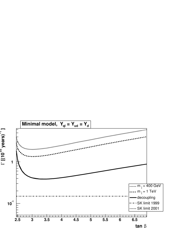
Figure 2: Decay rate $\Gamma(p\to K^{+}\bar{\nu})$ as function of $\tan\beta$ in the minimal model with $Y_{ql}=Y_{ud}=Y_{d}$. The experimental limits are given by SuperKamiokande experiment [20, 21].

We choose the parameters in eqn. (17) as described in Section 3 and vary $\tan\beta$. Since the decay width is proportional to $\tan\beta$, low values are preferred to obtain a small decay rate. On the one hand, the top Yukawa coupling becomes non-perturbative for low $\tan\beta$ since $h_{t}\simeq\frac{1}{\sin\beta}$. Hence, we start at $\tan\beta\simeq 2.5$. Fig. 2 shows the results of the following three cases: (i) all sfermions have masses of 1 TeV; (ii) $m_{\tilde{t}}$ is changed to 400 GeV; (iii) decoupling scenario, where the scalars of the first and second generation have masses of 10 TeV. The dash-dotted line represents the experimental limit $\tau=6.7\times 10^{32}$ years as given by the SuperKamiokande experiment [20, 17], the dotted line is the new limit $\tau=1.9\times 10^{33}$ years [21]. As in refs. [3, 4], the amplitude is always above the experimental limit.

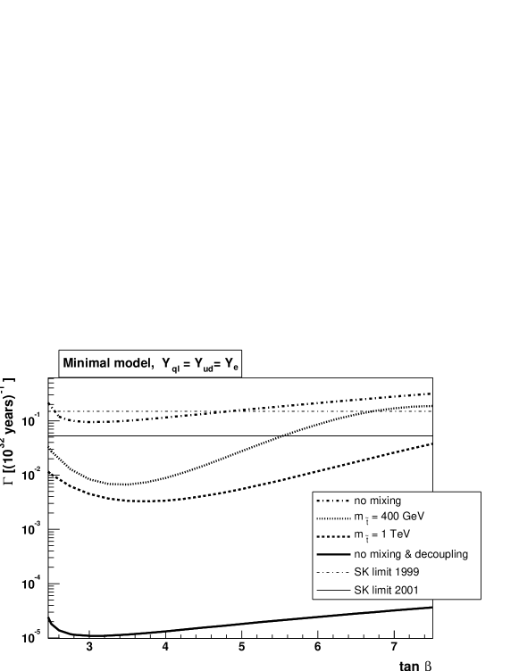
Figure 3: Decay rate $\Gamma(p\to K^{+}\bar{\nu})$ as a function of $\tan\beta$ with $Y_{ql}=Y_{ud}=Y_{e}$. The mixing matrix ${\cal M}$ is taken arbitrary or ${\cal M}=\mathbbm{1}$.

Next, we study the case

$$Y_{qq}=Y_{ue}=Y_{u}\ ,\qquad Y_{ql}=Y_{ud}=Y_{e}\ ,$$ (24)

in order to illustrate the strong dependence of the decay rate on flavour mixing and therefore on Yukawa unification. The Wilson coefficients now read

$$\begin{split}C_{5L}^{u}&=({\cal D}_{u}\,P)({\cal M}\,{\cal D}_{e})\ ,\\ C_{5R}^{u}&=({\cal D}_{u}\,{\cal M}^{*})(P^{*}\,{\cal M}{\cal D}_{e})\end{split}$$ (25)

and

$$\begin{split}C_{5L}^{d}&=({\cal M}^{T}P\,{\cal D}_{u}{\cal M})({\cal D}_{e})\ ,\\ C_{5R}^{d}&=(P^{*}{\cal M}^{*}{\cal D}_{e})({\cal M}^{T}{\cal D}_{u})\ ,\end{split}$$ (26)

where ${\cal M}=U_{u}^{\dagger}\,U_{e}$ replaces the CKM matrix $V_{\text{\sc ckm}}$. Note that the mixing matrix in $Y_{u}$ or $Y_{d}$ (cf. eqs. (A.3) and (A.4)) is still given by $V_{\text{\sc ckm}}$. Since $Y_{d}\not=Y_{e}$, the masses and mixing of quarks and leptons are different and ${\cal M}$ is undetermined.

We first ignore mixing, i.e. ${\cal M}=\mathbbm{1}$, and calculate the decay rate; the results are shown in fig. 3. Without mixing, only scalars of the first and second generation take part so that the decay rate can be reduced significantly in the decoupling scenario where the triangle diagram factor (13) changes by almost two orders of magnitude.

Now we take ${\cal M}$ totally arbitrarily and minimize the decay rate. As can be seen in fig. 3, it is possible to push the amplitude below the experimental limit even for smaller sfermion masses. In the case $m_{\tilde{t}}=400$ GeV, this is only possible for small values of $\tan\beta$. The fact that a sufficiently low decay rate can be found illustrates the dependence on flavour mixing and therefore the uncertainty due to the failure of Yukawa unification.

4.2 Consistent model

In this case the coefficients of the operators can be derived from the superpotential (8),

$$\begin{split}Y_{qq}&=Y_{1}-2\frac{\sigma}{M_{\text{Pl}}}f_{1}^{S}-\frac{1}{2}\frac{\sigma}{M_{\text{Pl}}}f_{2}^{S}\ ,\\ Y_{ue}&=Y_{1}-2\frac{\sigma}{M_{\text{Pl}}}f_{1}^{S}-\frac{1}{2}\frac{\sigma}{M_{\text{Pl}}}\left(f_{2}^{S}+5f_{2}^{A}\right)\end{split}$$ (27)

and

$$\begin{split}Y_{ql}&=Y_{2}+2\frac{\sigma}{M_{\text{Pl}}}h_{1}-3\frac{\sigma}{M_{\text{Pl}}}h_{2}\ ,\\ Y_{ud}&=Y_{2}+2\frac{\sigma}{M_{\text{Pl}}}h_{1}+2\frac{\sigma}{M_{\text{Pl}}}h_{2}\ .\end{split}$$ (28)

Note that $Y_{ql}-Y_{ud}=Y_{e}-Y_{d}$, which means that $Y_{ql}$ and $Y_{ud}$ cannot be zero at the same time.

It is instructive to express these Yukawa matrices in terms of the quark and charged lepton Yukawa couplings and the additional matrices $f$ and $h$ (cf. relations eqs. (A.5)),

$$\begin{split}Y_{qq}=Y_{qq}^{S}=Y_{ue}^{S}&=Y_{u}^{S}-5\frac{\sigma}{M_{\text{Pl}}}\left(f_{1}^{S}+\frac{1}{4}f_{2}^{S}\right)\ ,\\ Y_{ue}^{A}&=Y_{u}^{A}-\frac{5}{2}\,\frac{\sigma}{M_{\text{Pl}}}f_{2}^{A}\ ,\\ Y_{ql}&=Y_{e}+5\frac{\sigma}{M_{\text{Pl}}}h_{1}\ ,\\ Y_{ud}&=Y_{d}+5\frac{\sigma}{M_{\text{Pl}}}h_{1}\ .\end{split}$$ (29)

If one allows the (3,3)-component of $f_{1}$ and $f_{2}$ to be ${\cal O}(\frac{M_{\text{Pl}}}{\sigma})\gg 1$, proton decay via dimension five operators can be avoided, for instance, by satisfying

$$f_{1}^{S}+\frac{1}{4}f_{2}^{S}=\frac{M_{\text{Pl}}}{5\,\sigma}\,Y_{u}^{S}\ ,\qquad f_{2}^{A}=\frac{2}{5}\,\frac{M_{\text{Pl}}}{\sigma}\,Y_{u}^{A}$$ (30)

so that both $C_{5L}=Y_{qq}Y_{ql}$ and $C_{5R}=Y_{ue}Y_{ud}$ vanish.

Even if we restrict ourselves to ‘natural matrices’, i.e. couplings ${\cal O}(1)$, we can considerably reduce the decay amplitudes by a suitable choice of matrices. In the following, we will illustrate this with two simple examples where either the $RRRR$ or the $LLLL$ contribution vanishes at the GUT scale.

The first model is given by

$$\begin{split}Y_{qq}=Y_{ue}&=\operatorname{diag}(0,0,y_{t})\ ,\\ Y_{ud}&=\operatorname{diag}(0,y_{s}-y_{\mu},y_{b}-y_{\tau})\ ,\\ Y_{ql}&=\operatorname{diag}(y_{e}-y_{d},0,0)\ ,\end{split}$$ (31)

where $y_{j}$ are the Yukawa couplings of the fermions at $M_{\text{GUT}}$. In this model the $RRRR$ contribution vanishes completely because $C_{5R}^{ijkm}=Y_{ue}^{ij}\ Y_{ud}^{km}$ is zero whenever a particle of the first generation takes part. But according to figs. 6(d) and 7(b), at least one particle of the first generation is needed. Furthermore, only the decay channel $p\to K\bar{\nu}_{e}$ remains. As requested, all matrix elements are ${\cal O}(1)$ or smaller.

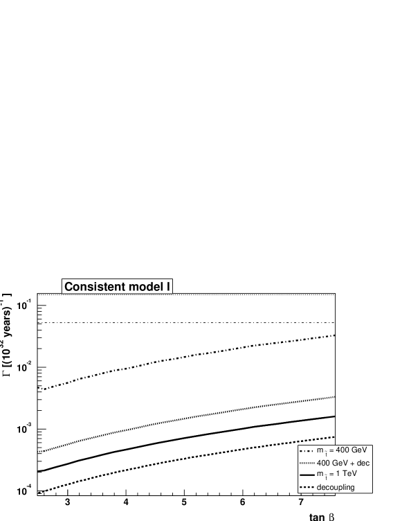
Figure 4: Decay rate $\Gamma(p\to K^{+}\bar{\nu})$ as function of $\tan\beta$ in the consistent model.

After RGE evolution by means of eqs. (B.3) and (B.4), the simple structure of Wilson coefficients changes slightly, but the $RRRR$ contribution and the decay channel $p\to K\bar{\nu}_{\mu}$ are still negligible whereas $p\to K\bar{\nu}_{\tau}$ becomes dominant. Fig. 4 shows the results for different sfermion masses. The decay amplitude is always well below the experimental limit, in the case $m_{\tilde{t}}=1$ TeV even more than two orders of magnitude.

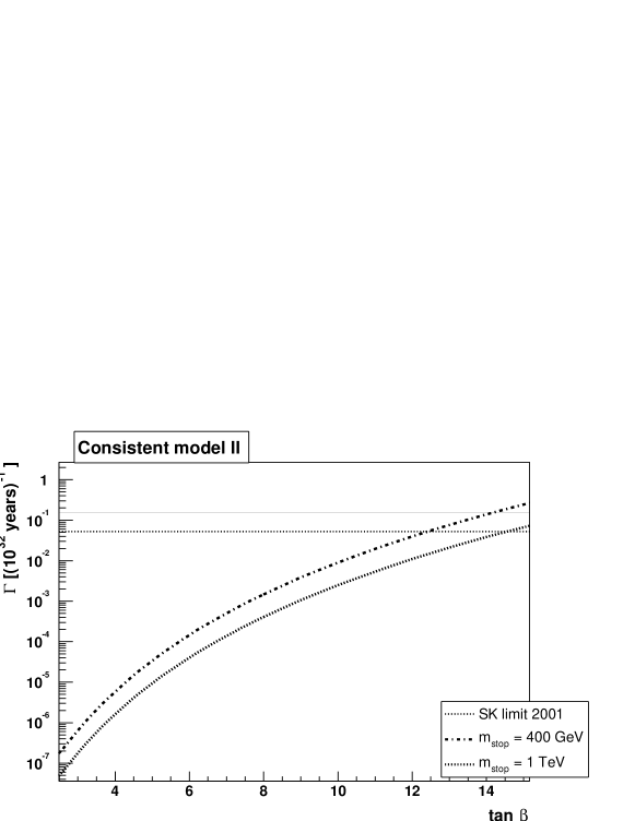
Figure 5: Decay rate $\Gamma(p\to K^{+}\bar{\nu})$ in the second model.

Now we turn to the second model where the $LLLL$ contribution vanishes at $M_{\text{GUT}}$,

$$\begin{split}Y_{qq}=Y_{ue}&=\operatorname{diag}(0,0,y_{t})\ ,\\ Y_{ud}&=\operatorname{diag}(y_{d}-y_{e},y_{s}-y_{\mu},y_{b})\ ,\\ Y_{ql}&=\operatorname{diag}(0,0,y_{\tau})\ .\end{split}$$ (32)

Now $C_{5L}^{ijkm}=Y_{qq}^{ij}\ Y_{ql}^{km}$ is only different from zero for $i=j=k=m=3$ and the decay has to be non-diagonal. Only the $RRRR$ contribution with a low absolute value remains. After renormalization, the $RRRR$ contribution is still dominated by third generation scalars so that decoupling of the first and second generation does not change the result. The $LLLL$ operator contributes only via $p\to K\bar{\nu}_{\tau}$.

As shown in fig. 5, the proton decay rate is even smaller in this model. Furthermore, due to the smaller (3,3)-component of $h_{1}$ compared to the first model, it can easily be used for higher values of $\tan\beta$.

4.3 Proton decay via dimension six operators

For completeness we include proton decay via X and Y bosons [22, 23]. The dominant decay mode is $p\to e^{+}\pi^{0}$. The decay width is given by

$$\Gamma(p\to e^{+}\pi^{0}) =\frac{m_{p}}{64\pi f_{\pi}^{2}}\,\alpha^{2}(1+D+F)^{2}\,\Bigl{(}\frac{g_{u}^{2}}{M_{V}^{2}}A\Bigl{)}^{2}\,\Bigl{[}\,1+\big{(}\,1+\left|V_{ud}\right|^{2}\big{)}^{2}\Bigl{]}\;.$$ (33)

The enhancement factor $A$ contains both a short-distance contribution $A^{\text{SD}}$ between the SUSY-breaking and GUT scales and a long-distance contribution $A^{\text{LD}}\equiv A_{l}$ between 1 GeV and the SUSY-breaking scale. $A^{\text{SD}}$ splits into three parts according to the three gauge couplings:

$$A^{\text{SD}}=\biggl{[}\frac{\alpha_{1}(M_{Z})}{\alpha_{5}}\biggl{]}^{\frac{23}{30\,b_{1}}}\biggl{[}\frac{\alpha_{2}(M_{Z})}{\alpha_{5}}\biggl{]}^{\frac{3}{2\,b_{2}}}\biggl{[}\frac{\alpha_{3}(M_{Z})}{\alpha_{5}}\biggl{]}^{\frac{4}{3\,b_{3}}}=2.37\ ,$$ (34)

where the first part is an approximate calculation [24].

With the Super-Kamiokande limit $\tau(p\to e^{+}\pi^{0})=5.3\times 10^{33}$ years [25] and using $\alpha=0.015\,\text{GeV}^{3}$ of ref. [14], the mass of the heavy gauge bosons has to satisfy the lower bound

$$M_{V}\geq 6.8\times 10^{15}\,\text{GeV}\ ,$$ (35)

roughly half of $M_{\text{GUT}}$ (20). Since $\tau\propto M_{V}^{4}$, the proton decay rate for $M_{V}=M_{\text{GUT}}$ is far below the detection limit which can be reached within the next years.

5 Conclusion

We have recalculated the proton decay rate in supersymmetric SU(5) GUTs. In particular, we have emphasized the strong dependence of the decay amplitude for flavour mixing.

Minimal SU(5) GUT is inconsistent since the predicted Yukawa unification, $Y_{d}=Y_{e}$, is badly violated. A consistent supersymmetric SU(5) model requires additional interactions which account for the difference of down quark and charged lepton masses. Such interactions are conveniently parameterized by higher dimensional operators.

We have shown that such operators can reduce the proton decay rate by several orders of magnitude and make it consistent with the experimental upper bound. We are not aware of a mechanism which would naturally lead to the required relations among Yukawa couplings. But, on the other hand, proton decay also does not rule out consistent supersymmetric SU(5) models.

Acknowledgements

We are very grateful to Wilfried Buchmüller for his guidance in this project. The work of D.E.C. was supported by Fundação para a Ciência e a Tecnologia under the grant SFRH/BPD/1598/2000.

Appendix A The SU(5) Yukawa sector and specific bases

Minimal model

In the minimal theory, the SU(5) Yukawa sector of the superpotential reads

$$W_{Y}=\tfrac{1}{4}\,Y_{1}^{ij}\,\mathsf{10}_{i}\;\mathsf{10}_{j}\;H(\mathsf{5})+\sqrt{2}\,Y_{2}^{ij}\,\mathsf{10}_{i}\;\mathsf{5}^{*}_{j}\;\overline{H}(\mathsf{5}^{*})\ .$$

From the superpotential one can immediately conclude that $Y_{1}$ is a symmetric complex matrix. With $Y_{u}=Y_{1}$ and $Y_{d}=Y_{2}$, the Yukawa matrices have the form

$$Y_{u} =U_{u}\,{\cal D}_{u}\,P\,U_{u}^{\top}\ ,$$

$$Y_{d} =U_{d}\,{\cal D}_{d}\,U_{d\,R}^{\dagger}\ .$$

Here, $P$ is an additional phase matrix with $\det P=1$ which is usually parametrized as

$$P=e^{i\,\varphi}\,\operatorname{diag}(e^{i\phi_{13}},e^{i\phi_{23}},1)\ .$$ (A.1)

These phases cannot be absorbed by field redefinitions [23]. The CKM matrix is then defined as

$$V_{\text{\sc ckm}}=U_{u}^{\dagger}\,U_{d}\ .$$ (A.2)

The most general weak basis transformation which leaves the interactions invariant is:

$$\mathsf{10}_{i} \to\mathsf{10}^{\prime}_{j}={\cal U}_{ij}\mathsf{10}_{j}\ ,$$

$$\mathsf{5}^{*}_{i} \to\mathsf{5}^{*\,\prime}_{j}={\cal V}_{ij}\mathsf{5}^{*}_{j}\ .$$

Then the Yukawa matrices transform like

$$Y_{u} \to{\cal U}^{\top}\,Y_{u}\,{\cal U}\ ,$$

$$Y_{d} \to{\cal U}^{\top}\,Y_{d}\,{\cal V}\ .$$

The superpotential of the SU(5) Yukawa interactions expressed in terms of SM superfields is given by eqn. (4). Transforming the singlets fields by $\Phi\to{\cal W}_{\Phi}\Phi$, the superpotential transforms like

$$W_{Y}=\; Q^{\top}\,({\cal U}^{\top}\,Y_{u}\,{\cal U}\,{\cal W}_{u})\,u^{\text{\sc c}}\,H_{f}+Q^{\top}\,({\cal U}^{\top}\,Y_{d}\,{\cal V}\,{\cal W}_{d})\,d^{\text{\sc c}}\,\overline{H}_{f}+e^{\text{\sc c}\top}\,({\cal W}_{e}^{\top}\,{\cal U}^{\top}\,Y_{e}\,{\cal V})\,L\,\overline{H}_{f}$$

$$+\tfrac{1}{2}\,Q^{\top}\,({\cal U}^{\top}\,Y_{qq}\,{\cal U})\,Q\,H_{\text{\sc c}}+Q^{\top}\,({\cal U}^{\top}\,Y_{ql}\,{\cal V})\,L\,\overline{H}_{\text{\sc c}}$$

$$+u^{\text{\sc c}\top}\,({\cal W}_{u}^{\top}\,{\cal U}^{\top}\,Y_{ue}\,{\cal U}\,{\cal W}_{e})\,e^{\text{\sc c}}\,H_{\text{\sc c}}+u^{\text{\sc c}\top}\,({\cal W}_{u}^{\top}\,{\cal U}^{\top}\,Y_{ud}\,{\cal V}\,{\cal W}_{d})\,d^{\text{\sc c}}\,\overline{H}_{\text{\sc c}}\ .$$

There are two possible physical bases now, namely diagonal up quark and diagonal down quark matrices, which can be realized by a suitable choice of all transformation matrices. With $Y_{qq}=Y_{ue}=Y_{u}$ and $Y_{ql}=Y_{ud}=Y_{d}$, the Yukawa interactions read

$$\begin{split}W_{Y}=\;&Q^{\top}\,{\cal D}_{u}\,u^{\text{\sc c}}\,H_{f}+Q^{\top}\,(V_{\text{\sc ckm}}\,{\cal D}_{d})\,d^{\text{\sc c}}\,\overline{H}_{f}+e^{\text{\sc c}\top}\,{\cal D}_{e}\,L\,\overline{H}_{f}\\ &+\tfrac{1}{2}\,Q^{\top}\,({\cal D}_{u}\,P)\,Q\,H_{\text{\sc c}}+Q^{\top}\,(V_{\text{\sc ckm}}\,{\cal D}_{d})\,L\,\overline{H}_{\text{\sc c}}\\ &+u^{\text{\sc c}\top}\,({\cal D}_{u}\,V_{\text{\sc ckm}}^{*})\,e^{\text{\sc c}}\,H_{\text{\sc c}}+u^{\text{\sc c}\top}\,(P^{*}\,V_{\text{\sc ckm}}\,{\cal D}_{d})\,d^{\text{\sc c}}\,\overline{H}_{\text{\sc c}}\end{split}$$ (A.3)

in the first and

$$\begin{split}W_{Y}=\;&Q^{\top}\,(V_{\text{\sc ckm}}^{\dagger}\,{\cal D}_{u})\,u^{\text{\sc c}}\,H_{f}+Q^{\top}\,{\cal D}_{d}\,d^{\text{\sc c}}\,\overline{H}_{f}+e^{\text{\sc c}\top}\,{\cal D}_{e}\,L\,\overline{H}_{f}\\ &+\tfrac{1}{2}\,Q^{\top}\,(V_{\text{\sc ckm}}^{\dagger}\,{\cal D}_{u}\,P\,V_{\text{\sc ckm}}^{*})\,Q\,H_{\text{\sc c}}+Q^{\top}\,{\cal D}_{d}\,L\,\overline{H}_{\text{\sc c}}\\ &+u^{\text{\sc c}\top}\,({\cal D}_{u}\,V_{\text{\sc ckm}}^{*})\,e^{\text{\sc c}}\,H_{\text{\sc c}}+u^{\text{\sc c}\top}\,(P^{*}\,V_{\text{\sc ckm}}\,{\cal D}_{d})\,d^{\text{\sc c}}\,\overline{H}_{\text{\sc c}}\end{split}$$ (A.4)

in the second basis. The former is used in ref. [10], the latter in ref. [3].

In principle, these formulae are only valid for unbroken supersymmetry where one can use the same transformations for the fermions and their supersymmetric partners. Broken supersymmetry gives small corrections to these transformations [9].

Consistent model

Expanding the superpotential by higher dimensional operators, the identities (5) and (6),

$$Y_{u}=Y_{qq}=Y_{ue}=Y_{1}\ ,\qquad Y_{d}=Y_{ql}=Y_{ud}=Y_{2}\ ,$$

at $M_{\text{GUT}}$ no longer hold. Instead, one can derive the following relations between the matrices:

$$\begin{split}Y_{qq}-Y_{ue}&=\frac{5}{2}\frac{\sigma}{M_{\text{Pl}}}f_{2}^{A}\ ,\\ Y_{u}-Y_{qq}&=5\frac{\sigma}{M_{\text{Pl}}}f_{1}^{S}+\frac{5}{4}\frac{\sigma}{M_{\text{Pl}}}\left(f_{2}^{S}+f_{2}^{A}\right)\ ,\\ Y_{u}-Y_{ue}&=5\frac{\sigma}{M_{\text{Pl}}}f_{1}^{S}+\frac{5}{4}\frac{\sigma}{M_{\text{Pl}}}\left(f_{2}^{S}+3f_{2}^{A}\right)\ ,\\ Y_{d}-Y_{e}=Y_{ud}-Y_{ql}&=5\frac{\sigma}{M_{\text{Pl}}}h_{2}\ ,\\ \tfrac{3}{5}Y_{d}+\tfrac{2}{5}Y_{e}&=Y_{2}-3\frac{\sigma}{M_{\text{Pl}}}h_{1}\ ,\\ Y_{ql}-Y_{e}=Y_{ud}-Y_{d}&=5\frac{\sigma}{M_{\text{Pl}}}h_{1}\ .\end{split}$$ (A.5)

The antisymmetric part of $f_{2}$ is determined by the difference between $Y_{qq}$ and $Y_{ue}$, then only symmetric terms of $f_{1}$ and $f_{2}$ remain.

Appendix B Renormalization group equations

Yukawa couplings

The one-loop renormalization group equations, in the $\overline{\text{\rm MS}}$ scheme, can be written for general Yukawa matrices [26]

$$\begin{split}16\pi^{2}\frac{d\,Y_{u}}{dt}&=\left[\,T_{u}-G_{u}(t)+\frac{3}{2}\left(b\,Y_{u}\,Y_{u}^{\dagger}+c\,Y_{d}\,Y_{d}^{\dagger}\right)\right]Y_{u}\ ,\\ 16\pi^{2}\frac{d\,Y_{d}}{dt}&=\left[\,T_{d}-G_{d}(t)+\frac{3}{2}\left(b\,Y_{d}\,Y_{d}^{\dagger}+c\,Y_{u}\,Y_{u}^{\dagger}\right)\right]Y_{d}\ ,\\ 16\pi^{2}\frac{d\,Y_{e}}{dt}&=Y_{e}\,\left(\,T_{e}-G_{e}(t)+\frac{3}{2}b\,Y_{e}^{\dagger}\,Y_{e}\right)\ ,\end{split}$$ (B.1)

where $t=\log\mu/M_{Z}$ and the traces $T_{u},T_{d},T_{e}$ are given by

$$\begin{split}T_{u}&=\operatorname{tr}\,(3\,Y_{u}\,Y_{u}^{\dagger}+3\,a\,Y_{d}\,Y_{d}^{\dagger}+a\,Y_{e}^{\dagger}\,Y_{e})\ ,\\ T_{d}=T_{e}&=\operatorname{tr}\,(3\,a\,Y_{u}\,Y_{u}^{\dagger}+3\,Y_{d}\,Y_{d}^{\dagger}+\,Y_{e}^{\dagger}\,Y_{e})\ .\end{split}$$ (B.2)

The constants $a$, $b$ and $c$ as well as the functions $G_{u}(t)$, $G_{d}(t)$ and $G_{e}(t)$, are summarized in the table 1.

	SM	MSSM
$\cfrac{1}{2}$ (a, b, c)	(1, 1, $-\frac{3}{2}$)	(0, 2, 1)
$\cfrac{1}{2}$ $G_{u}(t)$	$\tfrac{17}{20}\,g_{1}^{2}(t)+\tfrac{9}{4}\,g_{2}^{2}(t)+8\,g_{3}^{2}(t)\qquad$	$\tfrac{13}{15}\,g_{1}^{2}(t)+3\,g_{2}^{2}(t)+\tfrac{16}{3}\,g_{3}^{2}(t)$
$\cfrac{1}{2}$ $G_{d}(t)$	$\tfrac{1}{4}\,g_{1}^{2}(t)+\tfrac{9}{4}\,g_{2}^{2}(t)+8\,g_{3}^{2}(t)$	$\tfrac{7}{15}\,g_{1}^{2}(t)+3\,g_{2}^{2}(t)+\tfrac{16}{3}\,g_{3}^{2}(t)$
$\cfrac{1}{2}$ $G_{e}(t)$	$\tfrac{9}{4}\,g_{1}^{2}(t)+\tfrac{9}{4}\,g_{2}^{2}(t)$	$\tfrac{9}{5}\,g_{1}^{2}(t)+3\,g_{2}^{2}(t)$
$\cfrac{1}{2}$ $b_{1}$	$\tfrac{4}{3}n+\tfrac{1}{10}m$	$2\,n+\tfrac{3}{10}m$
$\cfrac{1}{2}$ $b_{2}$	$\tfrac{4}{3}n+\tfrac{1}{6}m-\tfrac{22}{3}$	$2\,n+\tfrac{1}{2}m-6$
$\cfrac{1}{2}$ $b_{3}$	$\tfrac{4}{3}n-11$	$2\,n-9$

Table 1: Coefficients to (B.1) and (B.2). The running gauge coupling constant at 1-loop is given by $g^{2}_{i}(t)=g^{2}_{i}(0)/\left(1-\frac{b_{i}}{8\pi^{2}}\,g^{2}_{i}(0)\,t\right)$. The integers $n$ and $m$ stand for number of generations and Higgs doublets, respectively.

The equations for the Wilson coefficients read [3]

$$\begin{split}16\pi^{2}\frac{d}{dt}C_{5L}^{ijkl}&=\left(-8\,g_{3}^{2}-6\,g_{2}^{2}-\tfrac{2}{3}g_{1}^{2}\right)C_{5L}^{ijkl}+C_{5L}^{mjkl}\!\left(\!Y_{d}Y_{d}^{\dagger}+Y_{u}Y_{u}^{\dagger}\right)^{i}_{m}\\ &\quad+C_{5L}^{imkl}\!\left(Y_{e}^{\dagger}Y_{e}\right)_{m}^{j}\!\!+C_{5L}^{ijml}\!\left(\!Y_{d}Y_{d}^{\dagger}+Y_{u}Y_{u}^{\dagger}\right)^{k}_{m}\!\!+C_{5L}^{ijkm}\!\left(\!Y_{d}Y_{d}^{\dagger}+Y_{u}Y_{u}^{\dagger}\right)^{l}_{m},\end{split}$$ (B.3)

$$\begin{split}16\pi^{2}\frac{d}{dt}C_{5R}^{ijkl}&=\left(-8\,g_{3}^{2}-4\,g_{1}^{2}\right)C_{5R}^{ijkl}+C_{5R}^{mjkl}\left(2\,Y_{u}^{\dagger}Y_{u}\right)_{m}^{i}\\ &\quad+C_{5R}^{imkl}\left(2\,Y_{d}^{\dagger}Y_{d}\right)_{m}^{j}+C_{5R}^{ijml}\left(2\,Y_{e}Y_{e}^{\dagger}\right)^{k}_{m}+C_{5R}^{ijkm}\left(2\,Y_{u}^{\dagger}Y_{u}\right)_{m}^{l}.\end{split}$$ (B.4)

Gauge couplings, Constraint on $M_{H_{\text{\sc c}}}$

In minimal supersymmetric SU(5), the RGE at one-loop level are given by [10]:

$$\alpha_{1}^{-1}(M_{Z})=\alpha_{5}^{-1}(\Lambda)+\frac{1}{2\pi}\biggl{[}\left(-\frac{2}{3}n-\frac{1}{2}\right)\log\frac{M_{S}}{M_{Z}}+\left(2n+\frac{3}{5}\right)\log\frac{\Lambda}{M_{Z}}-10\log\frac{\Lambda}{M_{V}}+\frac{2}{5}\log\frac{\Lambda}{M_{H_{\text{\sc c}}}}\biggl{]},$$

$$\alpha_{2}^{-1}(M_{Z})=\alpha_{5}^{-1}(\Lambda)+\frac{1}{2\pi}\biggl{[}\left(-\frac{2}{3}n-\frac{13}{6}\right)\log\frac{M_{S}}{M_{Z}}+\left(2n-5\right)\log\frac{\Lambda}{M_{Z}}-6\log\frac{\Lambda}{M_{V}}+2\log\frac{\Lambda}{M_{3}}\biggl{]},$$

$$\alpha_{3}^{-1}(M_{Z})\!=\!\alpha_{5}^{-1}(\Lambda)+\frac{1}{2\pi}\biggl{[}\left(-\frac{2}{3}n\!-\!2\right)\log\frac{M_{S}}{M_{Z}}+\left(2n\!-\!9\right)\log\frac{\Lambda}{M_{Z}}-4\log\frac{\Lambda}{M_{V}}+3\log\frac{\Lambda}{M_{8}}+\log\frac{\Lambda}{M_{H_{\text{\sc c}}}}\biggl{]},$$

where $M_{S}$ is the SUSY breaking scale. Using the combinations

$$(-\alpha_{1}^{-1}+3\alpha_{2}^{-1}-2\alpha_{3}^{-1})\;(M_{Z}) =\frac{1}{2\pi}\left[-2\,\log\frac{M_{S}}{M_{Z}}+\frac{12}{5}\log\left(\frac{M_{H_{\text{\sc c}}}}{M_{Z}}\left(\frac{M_{3}}{M_{8}}\right)^{\frac{5}{2}}\right)\right]\ ,$$ (B.5)

$$(5\alpha_{1}^{-1}-3\alpha_{2}^{-1}-2\alpha_{3}^{-1})\;(M_{Z}) =\frac{1}{2\pi}\left[8\,\log\frac{M_{S}}{M_{Z}}+12\,\log\frac{M_{V}^{2}\sqrt{M_{3}M_{8}}}{M_{Z}^{3}}\right]$$ (B.6)

one can derive constraints on the products $M_{H_{\text{\sc c}}}(M_{3}/M_{8})^{5/2}$ and $M_{V}^{2}\sqrt{M_{3}M_{8}}\equiv M_{\text{GUT}}^{3}$. At two-loop level, there are no simple analytic relations any more.

Taking $M_{8}=M_{3}=M_{\Sigma}$ as it was done for the constraint in eqs. (19) and (20), it simply reads $M_{H_{\text{\sc c}}}$ and $M_{\text{GUT}}^{3}=M_{V}^{2}M_{\Sigma}$.

Appendix C Diagrams

(a) $LLLL$ triangle diagrams

(b) $LLLL$ box diagrams

(c) $RRLL$ diagrams

(d) $RRRR$ diagrams

Figure 6: Diagrams with chargino dressing

(a) $LLLL$ diagrams

(b) $RRRR$ diagrams

Figure 7: Diagrams with neutralino dressing

Fig. 6 lists the diagrams for the decay $p\to K^{+}\bar{\nu}$ with chargino dressing; they are related to the first addend in (15). Those with right-handed fermions incoming can be divided into two groups depending on the dressing before (fig. 6(c)) or after the decay operator (fig. 6(d)); we therefore call them $RRLL$ and $RRRR$ diagrams, respectively. The latter case is the only one related to the $RRRR$ operator and $C_{5R}$ because there are no right-handed neutrinos in the model. As discussed in Section 3, the dimension five operators are flavour non-diagonal, hence several diagrams are suppressed.

By interchanging down and strange quarks as incoming and outgoing particles, we get the diagrams due to the second addend. The diagrams of the last one cannot be realized by chargino exchange, so we look at those with neutralino exchange that are given in fig. 7.

The coefficients $C_{LL}$ and $C_{RL}$ used in eqn. (15) then read

$$C_{LL/RL}=\frac{{\cal K}}{M_{H_{\text{\sc c}}}}\,C_{5L/5R}\,A_{s}\,A_{l}\,f(M;m_{1},m_{2})$$ (C.1)

where $C_{5L}=Y_{qq}Y_{ql}$ is related to $C_{LL}$ and $C_{5R}=Y_{ue}Y_{ud}$ to $C_{RL}$. They are evaluated at the GUT scale and $A_{s}$ gives the correction due to running from GUT to SUSY breaking scale where ${\cal K}$ is determined. In practice, the Wilson coefficients $C_{5}$ are renormalized by means of eqn. (B.3) and (B.4) and evaluated at SUSY breaking scale. Finally, $A_{l}$ describes the renormalization of the $d=6$ coefficients down to 1 GeV.

Appendix D Renormalization factors

The renormalization factors are crucial for analyzing the proton decay. Since there is some discrepancy in the literature, we want to discuss them here in detail.

As already mentioned in Section 3, there are two ranges for the renormalization, namely the short-distance between $M_{\text{GUT}}$ and $M_{\text{SUSY}}$ and the long-distance between the latter and the proton mass at $\sim$ 1 GeV leading to the factors $A_{s}$ and $A_{l}$. The former is highly dependent on the top Yukawa coupling $y_{t}$ and can therefore not be calculated analytically.

The renormalization group effects in SUSY GUTs have first been discussed in ref. [27]. At that time, not only the high top mass was unknown ($m_{t}=20\,$GeV was assumed), but since there were no data at $M_{Z}$, the values at 1 GeV were taken to calculate the decay rate. Hence the renormalization factors $A_{S}$ and $A_{L}$ were defined, which include the running factor of the Yukawa couplings from low to high scale. In this work, we use the Yukawa couplings at $M_{Z}$ and $M_{\text{SUSY}}$ and evaluate their values at $M_{\text{GUT}}$. These are taken as input parameters for the calculation, so our factors $A_{s}$ and $A_{l}$ differ from $A_{S}$ and $A_{L}$ in ref. [27, 10]. For the long-distance part, this discrepancy was stressed in ref. [28].

Because of the high top mass, $A_{s}$ cannot be solved analytically [10] and depends on the related particles. Hence the Wilson coefficients are evolved down to $M_{\text{SUSY}}$ by using eqs. (B.3) and (B.4). For simplicity, $M_{\text{SUSY}}$ is identified with the electroweak scale, so $A_{l}$ describes pure QCD renormalization down to 1 GeV,

$$A_{l}=\biggl{[}\frac{\alpha_{3}(\mu_{\text{had}})}{\alpha_{3}(M_{Z})}\biggl{]}^{\frac{6}{33-2n_{\!f}}}\to\biggl{[}\frac{\alpha_{3}(\mu_{\text{had}})}{\alpha_{3}(m_{c})}\biggl{]}^{\frac{2}{9}}\biggl{[}\frac{\alpha_{3}(\mu_{\text{c}})}{\alpha_{3}(m_{b})}\biggl{]}^{\frac{6}{25}}\biggl{[}\frac{\alpha_{3}(m_{b})}{\alpha_{3}(m_{Z})}\biggl{]}^{\frac{6}{23}}=1.43\ ,$$ (D.1)

with $\mu_{\text{had}}=1$ GeV.

References

-
[1]
S. Dimopoulos and H. Georgi,
Softly Broken Supersymmetry And SU(5),
Nucl. Phys. B 193 (1981) 150;
N. Sakai, Naturalness In Supersymmetric “GUTs”, Z. Phys. C 11 (1981) 153. - [2] For a recent review, see S. Raby, Proton decay, arXiv:hep-ph/0211024.
- [3] T. Goto and T. Nihei, Effect of RRRR dimension 5 operator on the proton decay in the minimal SU(5) SUGRA GUT model, Phys. Rev. D 59 (1999) 115009.
- [4] H. Murayama and A. Pierce, Not even decoupling can save minimal supersymmetric SU(5), Phys. Rev. D 65 (2002) 055009.
- [5] B. Bajc, P. F. Perez and G. Senjanovic, Proton decay in minimal supersymmetric SU(5), Phys. Rev. D 66 (2002) 075005.
- [6] B. Bajc, P. F. Perez and G. Senjanovic, Minimal supersymmetric SU(5) theory and proton decay: Where do we stand?, arXiv:hep-ph/0210374.
-
[7]
N. Sakai and T. Yanagida,
Proton Decay In A Class Of Supersymmetric Grand Unified
Models,
Nucl. Phys. B 197 (1982) 533;
S. Weinberg, Supersymmetry At Ordinary Energies. 1. Masses And Conservation Laws, Phys. Rev. D 26 (1982) 287. - [8] S. Dimopoulos, S. Raby and F. Wilczek, Proton Decay In Supersymmetric Models, Phys. Lett. B 112 (1982) 133.
- [9] P. Nath, A. H. Chamseddine and R. Arnowitt, Nucleon Decay In Supergravity Unified Theories, Phys. Rev. D 32 (1985) 2348.
- [10] J. Hisano, H. Murayama and T. Yanagida, Nucleon decay in the minimal supersymmetric SU(5) grand unification, Nucl. Phys. B 402 (1993) 46.
- [11] M. Claudson, M. B. Wise and L. J. Hall, Chiral Lagrangian For Deep Mine Physics, Nucl. Phys. B 195 (1982) 297.
- [12] S. Chadha and M. Daniel, Chiral Lagrangian Calculation Of Nucleon Decay Modes Induced By D = 5 Supersymmetric Operators, Nucl. Phys. B 229 (1983) 105.
- [13] S. J. Brodsky, J. R. Ellis, J. S. Hagelin and C. T. Sachrajda, Baryon Wave Functions And Nucleon Decay, Nucl. Phys. B 238 (1984) 561.
- [14] S. Aoki et al. [JLQCD Collaboration], Nucleon decay matrix elements from lattice QCD, Phys. Rev. D 62 (2000) 014506.
- [15] R. E. Shrock and L. L. Wang, A New Generalized Cabibbo Fit And Application To Quark Mixing Angles In The Sequential Weinberg-Salam Model, Phys. Rev. Lett. 41 (1978) 1692.
- [16] V. Lucas and S. Raby, Nucleon decay in a realistic SO(10) SUSY GUT, Phys. Rev. D 55 (1997) 6986.
- [17] K. Hagiwara et al. [Particle Data Group Collaboration], Review Of Particle Physics, Phys. Rev. D 66 (2002) 010001.
-
[18]
M. Dine, A. Kagan and S. Samuel,
Naturalness In Supersymmetry, Or Raising The Supersymmetry
Breaking Scale,
Phys. Lett. B 243 (1990) 250;
S. Dimopoulos and G. F. Giudice, Naturalness constraints in supersymmetric theories with nonuniversal soft terms, Phys. Lett. B 357 (1995) 573;
A. Pomarol and D. Tommasini, Horizontal symmetries for the supersymmetric flavor problem, Nucl. Phys. B 466 (1996) 3;
A. G. Cohen, D. B. Kaplan and A. E. Nelson, The more minimal supersymmetric standard model, Phys. Lett. B 388 (1996) 588. - [19] G. Altarelli, F. Feruglio and I. Masina, From minimal to realistic supersymmetric SU(5) grand unification, JHEP 0011 (2000) 040.
- [20] Y. Hayato et al. [Super-Kamiokande Collaboration], Search for proton decay through in a large water Cherenkov detector, Phys. Rev. Lett. 83 (1999) 1529.
- [21] K. S. Ganezer [Super-Kamiokande Collaboration], The Search For Nucleon Decay At Super-Kamiokande, Int. J. Mod. Phys. A 16S1B (2001) 855.
- [22] A. J. Buras, J. R. Ellis, M. K. Gaillard and D. V. Nanopoulos, Aspects Of The Grand Unification Of Strong, Weak And Electromagnetic Interactions, Nucl. Phys. B 135 (1978) 66.
- [23] J. R. Ellis, M. K. Gaillard and D. V. Nanopoulos, On The Effective Lagrangian For Baryon Decay, Phys. Lett. B 88 (1979) 320.
- [24] L. E. Ibanez and C. Munoz, Enhancement Factors For Supersymmetric Proton Decay In The Wess-Zumino Gauge, Nucl. Phys. B 245 (1984) 425.
- [25] Y. Suzuki et al. [TITAND Working Group Collaboration], Multi-Megaton water Cherenkov detector for a proton decay search: TITAND (former name: TITANIC), arXiv:hep-ex/0110005.
-
[26]
V. D. Barger, M. S. Berger and P. Ohmann,
Supersymmetric grand unified theories: Two loop evolution of
gauge and Yukawa couplings,
Phys. Rev. D 47 (1993) 1093;
Universal evolution of CKM matrix elements, Phys. Rev. D 47 (1993) 2038;
V. D. Barger, M. S. Berger, P. Ohmann and R. J. Phillips, Phenomenological implications of the m(t) RGE fixed point for SUSY Higgs boson searches, Phys. Lett. B 314 (1993) 351. - [27] J. R. Ellis, D. V. Nanopoulos and S. Rudaz, Guts 3: Susy Guts 2, Nucl. Phys. B 202 (1982) 43.
- [28] R. Dermisek, A. Mafi and S. Raby, SUSY GUTs under siege: Proton decay, Phys. Rev. D 63 (2001) 035001.