UCT-TP-263/04

Revised January 2005

Electromagnetic nucleon form factors from
QCD sum rules
H. Castillo ^(a),(b) , C.A. Dominguez ^(c), M. Loewe ^(a)

(a) Facultad de Física, Pontificia Universidad Católica de Chile, Casilla 306, Santiago 22, Chile.
(b) Departamento de Ciencias, Pontificia Universidad Católica del Perú, Apartado 1761, Lima, Perú.
(c) Institute of Theoretical Physics & Astrophysics, University of Cape Town, Rondebosch 7701, South Africa.

Abstract

The electromagnetic form factors of the nucleon, in the space-like region, are determined from three-point function Finite Energy QCD Sum Rules. The QCD calculation is performed to leading order in perturbation theory in the chiral limit, and to leading order in the non-perturbative power corrections. The results for the Dirac form factor, $F_{1}(q^{2})$, are in very good agreement with data for both the proton and the neutron, in the currently accessible experimental region of momentum transfers. This is not the case, though, for the Pauli form factor $F_{2}(q^{2})$, which has a soft $q^{2}$-dependence proportional to the quark condensate $<0|\bar{q}q|0>$.

The electromagnetic form factors of the nucleon have been studied in perturbative QCD (PQCD), together with QCD sum rule estimates of the nucleon wave functions [1]. Comparison with data is difficult due to the extreme asymptotic nature of these theoretical results. In fact, the onset of PQCD in exclusive reactions does not appear to be as precocious as in inclusive processes. In addition, these wave functions are affected by some unavoidable model dependency. In any case, the Dirac form factor $F_{1}(Q^{2})$ does exhibit the expected leading asymptotic $1/Q^{4}$ behaviour. However, the Pauli form factor $F_{2}(Q^{2})$ turns out to be of higher twist, and therefore not accessible in the standard PQCD approach. At current experimental space-like momentum transfers, the results from the standard hard-scattering approach for $F_{1}(Q^{2})$ do not compare favourably with the data. On the other hand, some recent light-cone QCD sum rule determinations appear to improve the agreement with data from within a factor 5-6 to within a factor of two [2]. The source of this persistent disagreement does not seem easy to identify. In view of this, it is desirable to attempt a QCD sum rule determination in a region of experimentally accessible momentum transfers, and without any reference to the concept of a wave function. In addition, one should employ sum rules of a type which would provide a clear insight into the source(s) of potential disagreement with experiment. This can be achieved e.g. by using Finite Energy Sum Rules (FESR). In fact, in this framework the power corrections involving the vacuum condensates decouple to leading order in PQCD. In other words, power corrections of different dimensionality contribute to different FESR.

In this note we determine the Dirac and Pauli electromagnetic nucleon form factors, in a wide range of (space-like) momentum transfers, in the framework of three-point function QCD-FESR of leading dimensionality. As is well known by now, this technique is based on the Operator Product Expansion (OPE) of current correlators at short distances, and on the notion of quark-hadron duality [3]. Analyticity and dispersion relations connect the QCD information in the OPE to hadronic parameters entering the corresponding spectral functions. We compute the QCD correlator to leading order in perturbative QCD in the chiral limit ($m_{u}=m_{d}=0$), and include the leading order non-perturbative power corrections proportional to the quark-condensate and the four-quark condensate (with no gluon exchange). We begin by considering the following three-point function (see Fig. 1)

$$\Pi_{\mu}(p^{2},p^{\prime 2},Q^{2})=i^{2}\!\int\!\!\mbox{d}^{4}x\!\!\int\!\!\mbox{d}^{4}y\;e^{i(p^{\prime}\cdot x-q\cdot y)}\,\langle 0\left|T\{\eta_{N}(x)J_{\mu}^{EM}(y)\bar{\eta}_{N}(0)\}\right|0\rangle\;,$$ (1)

where $Q^{2}\equiv-q^{2}=-(p^{\prime}-p)^{2}\geq 0$ is fixed, and

$$\eta_{N}(x)=\varepsilon_{abc}\left[u^{a}(x)(C\gamma_{\alpha})u^{b}(x)\right](\gamma^{5}\gamma^{\alpha}d^{c}(x))$$ (2)

is an interpolating current with nucleon (proton) quantum numbers; the neutron case $u\leftrightarrow d$ will be discussed at the end. In Eq.(1), $J^{\mu}_{EM}$ is the electromagnetic current

$$J_{EM}^{\mu}(y)=\frac{2}{3}\bar{u}(y)\gamma^{\mu}u(y)-\frac{1}{3}\bar{d}(y)\gamma^{\mu}d(y)\;.$$ (3)

The current Eq.(2) couples to a nucleon of momentum $p$ and polarization $s$ according to

$$\langle 0\left|\eta_{N}(0)\right|N(p,s)\rangle=\lambda_{N}u(p,s),$$ (4)

where $u(p,s)$ is the nucleon spinor, and $\lambda_{N}$, the current-nucleon coupling, is a phenomenological parameter a-priori unknown. This parameter can be estimated, e.g. using QCD sum rules for a two-point function involving the currents $\eta_{N}$ [3]-[4]. In this case one can determine the nucleon mass, as well as the coupling $\lambda_{N}$.
Concentrating first on the hadronic sector, and inserting a one-particle nucleon state in the three-point function (1) brings out the nucleon form factors $F_{1}(q^{2})$, and $F_{2}(q^{2})$, defined as

$$\langle N(k_{1}\,,s_{1})\left|J_{\mu}^{EM}(0)\right|N(k_{2}\,,s_{2})\rangle=\bar{u}_{N}(k_{1},s_{1})\left[F_{1}(q^{2})\gamma_{\mu}+\frac{i\kappa}{2M_{N}}F_{2}(q^{2})\sigma_{\mu\nu}q^{\nu}\right]u_{N}(k_{2},s_{2})\;,$$ (5)

where $q^{2}=(k_{2}-k_{1})^{2}$, and $\kappa$ is the anomalous magnetic moment in units of nuclear magnetons ($\kappa_{p}=1.79$ for the proton, and $\kappa_{n}=-1.91$ for the neutron). The form factors $F_{1,2}(q^{2})$ are related to the electric and magnetic (Sachs) form factors $G_{E}(q^{2})$, and $G_{M}(q^{2})$, measured in elastic electron-proton scattering experiments, according to

$$G_{E}(q^{2}) \equiv F_{1}(q^{2})+\frac{\kappa q^{2}}{(2m)^{2}}F_{2}(q^{2})\;,$$ (6)

$$G_{M}(q^{2}) \equiv F_{1}(q^{2})+\kappa F_{2}(q^{2})\;,$$ (7)

where $G_{E}^{p}(0)=1$, $G_{M}^{p}(0)=1+\kappa_{p}$ for the proton, and $G_{E}^{n}(0)=0$, $G_{M}^{n}(0)=\kappa_{n}$ for the neutron. Next, the hadronic spectral function is obtained after inserting a complete set of nucleonic states in (1), and computing the double discontinuity in the complex $p^{2}\equiv s$, ${p^{\prime}}^{2}\equiv s^{\prime}$ plane. For $s,s^{\prime}<2.1\,\mbox{GeV}^{2}$, i.e. below the Roper resonance, one can safely approximate the hadronic spectral function by the single-particle nucleon pole, followed by a continuum with thresholds $s_{0}$ and $s^{\prime}_{0}$ ($s_{0},s^{\prime}_{0}>M_{N}^{2}$). This hadronic continuum is expected to coincide numerically with the perturbative QCD (PQCD) spectral function (local duality). This procedure is standard in QCD sum rule applications, and leads to

$$\mbox{Im}\Pi_{\mu}(s,s^{\prime},Q^{2})\Big{|}_{HAD} =\pi^{2}\,\lambda_{N}^{2}\,\delta(s-M_{N}^{2})\delta(s^{\prime}-M_{N}^{2})$$ (8)

$$\times\Bigg{\{}F_{1}(q^{2})\left[/\!\!\!p^{\prime}\gamma_{\mu}/\!\!\!p+M_{N}(/\!\!\!p^{\prime}\gamma_{\mu}+\gamma_{\mu}/\!\!\!p)+M_{N}^{2}\gamma_{\mu}\right]$$

$$+\frac{i\kappa}{2M_{N}}F_{2}(q^{2})\left[/\!\!\!p^{\prime}\sigma_{\mu\nu}/\!\!\!p+M_{N}(/\!\!\!p^{\prime}\sigma_{\mu\nu}+\sigma_{\mu\nu}/\!\!\!p)+M_{N}^{2}\sigma_{\mu\nu}\right]q^{\nu}\Bigg{\}}\Theta\left(s_{0}-s\right)$$

$$+\mbox{Im}\Pi_{\mu}(s,s^{\prime},Q^{2})\Big{|}_{PQCD}\Theta\left(s-s_{0}\right)\;,$$

where we have set $s_{0}=s^{\prime}_{0}$ for simplicity.

Turning to the QCD sector, the three-point function (1) to leading order in perturbative QCD, and in the chiral limit, is given by

$$\Pi^{\mu}(p^{2},{p^{\prime}}^{2},Q^{2})=16\int\mbox{d}^{4}x\;\int\mbox{d}^{4}y\;e^{i(p^{\prime}\cdot x-q\cdot y)}\;\mbox{Tr}\left[\int\frac{\mbox{d}^{4}{k_{1}}}{(2\pi)^{4}}\frac{/\!\!\!k_{1}}{k_{1}^{2}}e^{-ik_{1}\cdot(x-y)}\gamma^{\mu}\;\right.$$ (9)

$$\left.\times\int\frac{\mbox{d}^{4}{k_{2}}}{(2\pi)^{4}}\frac{/\!\!\!k_{2}}{k_{2}^{2}}e^{-ik_{2}\cdot y}\gamma_{\nu}\int\frac{\mbox{d}^{4}{k_{3}}}{(2\pi)^{4}}\frac{/\!\!\!k_{3}}{k_{3}^{2}}e^{+ik_{3}\cdot x}\gamma_{\alpha}\right]\left(\gamma^{5}\gamma^{\alpha}\int\frac{\mbox{d}^{4}{k_{4}}}{(2\pi)^{4}}\frac{/\!\!\!k_{4}}{k_{4}^{2}}e^{-ik_{4}\cdot x}\gamma^{\nu}\gamma^{5}\right)$$

$$+\;4\int\mbox{d}^{4}x\int\mbox{d}^{4}y\;e^{i(p^{\prime}\cdot x-q\cdot y)}\;\mbox{Tr}\left[\int\frac{\mbox{d}^{4}{k_{4}}}{(2\pi)^{4}}\frac{/\!\!\!k_{4}}{k_{4}^{2}}e^{-ik_{4}\cdot x}\gamma_{\nu}\int\frac{\mbox{d}^{4}{k_{3}}}{(2\pi)^{4}}\frac{/\!\!\!k_{3}}{k_{3}^{2}}e^{+ik_{3}\cdot x}\gamma_{\alpha}\right]$$

$$\times\left(\gamma^{\alpha}\int\frac{\mbox{d}^{4}{k_{1}}}{(2\pi)^{4}}\frac{/\!\!\!k_{1}}{k_{1}^{2}}e^{-ik_{1}\cdot(x-y)}\gamma^{\mu}\int\frac{\mbox{d}^{4}{k_{2}}}{(2\pi)^{4}}\frac{/\!\!\!k_{2}}{k_{2}^{2}}e^{-ik_{2}\cdot y}\gamma^{\nu}\right).$$

After computing the traces and performing the momentum space integrations, Eq.(9) involves several Lorentz structures analogous to those entering the hadronic spectral function Eq. (8). Before invoking duality one needs to choose a particular Lorentz structure present in both (8) and (9). A convenient choice turns out to be $/\!\!\!p^{\prime}\gamma_{\mu}/\!\!\!p$, which allows to project $F_{1}(q^{2})$, as this structure does not appear multiplying $F_{2}(q^{2})$ in Eq.(8). An additional advantage of this choice is that the quark condensate contribution, to be discussed later, does not involve the structure $/\!\!\!p^{\prime}\gamma_{\mu}/\!\!\!p$, on account of vanishing traces. There is, though, a non-perturbative term involving this structure and proportional to the four-quark condensate. However, eventually this term will not contribute to the FESR as its double discontinuity vanishes. Hence, $F_{1}(q^{2})$ will only be dual to the PQCD expression. It must be pointed out that the PQCD spectral function contains the structure $/\!\!\!p^{\prime}\gamma_{\mu}/\!\!\!p$ explicitly, as well as implicitly, i.e. there are terms proportional to this structure which are generated only once the momentum-space integration is performed.
After a very lengthy calculation, the imaginary part of Eq.(9) is given by

$$\mbox{Im}\Pi^{\mu}(s,s^{\prime},Q^{2})=\left[\frac{4}{(2\pi)^{8}}(3\Omega_{1}+4\Omega_{2}-\Omega_{3})\right]\left(/\!\!\!p^{\prime}\gamma^{\mu}/\!\!\!p\right)+\ldots\;,$$ (10)

where

$$\Omega_{1}=\frac{{\pi}^{6}}{2}\,\left(Q^{2}+s-s^{\prime}-\frac{Q^{4}+2\,Q^{2}\,s+s^{2}-2\,s\,s^{\prime}-{s^{\prime}}^{2}}{{\sqrt{Q^{4}+{\left(s-s^{\prime}\right)}^{2}+2\,Q^{2}\,\left(s+s^{\prime}\right)}}}\right)\;,$$ (11)

$$\Omega_{2} = {\pi}^{6}\left\{\frac{\left(2\,Q^{2}+3\,s-3\,s^{\prime}\right)}{3}-\frac{\left[(Q^{2}+s)^{3}(2\,Q^{2}+3s)+3\,\left(Q^{6}-5Q^{2}s^{2}-4s^{3}\right)s^{\prime}\right]}{3{\left[Q^{4}+{(s-s^{\prime})}^{2}+2\,Q^{2}(s+s^{\prime})\right]}^{\frac{3}{2}}}\right.$$ (12)

$$+ \left.\frac{\left[(3Q^{2}-4s)(Q^{2}+3s){s^{\prime}}^{2}+7Q^{2}{s^{\prime}}^{3}+3{s^{\prime}}^{4}\right]}{3\left[Q^{4}+{(s-s^{\prime})}^{2}+2\,Q^{2}(s+s^{\prime})\right]^{\frac{3}{2}}}\right\}\;,$$

$$\Omega_{3} = \frac{-\left\{\pi^{6}\,\left[23\,Q^{2}+18\,\left(-s+s^{\prime}\right)\right]\right\}}{72}+\frac{\pi^{6}}{72\,\left[Q^{4}+\left(s-s^{\prime}\right)^{2}+2\,Q^{2}\,\left(s+s^{\prime}\right)\right]^{\frac{5}{2}}}$$ (13)

$$\times \left[\left(23\,Q^{2}-18\,s\right)\,\left(Q^{2}+s\right)^{5}+\left(Q^{2}+s\right)^{3}\,\left(133\,Q^{4}-169\,Q^{2}\,s+108\,s^{2}\right)\,s^{\prime}\right.$$

$$+ \left.2\,\left(160\,Q^{8}+6\,Q^{6}\,s+3\,Q^{4}\,s^{2}+40\,Q^{2}\,s^{3}-117\,s^{4}\right)\,{s^{\prime}}^{2}\right.$$

$$+ \left.2\,\left(205\,Q^{6}-61\,Q^{4}\,s-122\,Q^{2}\,s^{2}+108\,s^{3}\right)\,{s^{\prime}}^{3}\right.$$

$$+ \left.\left(295\,Q^{4}-37\,Q^{2}\,s-54\,s^{2}\right)\,{s^{\prime}}^{4}+\left(113\,Q^{2}-36\,s\right)\,{s^{\prime}}^{5}+18\,{s^{\prime}}^{6}\right]\;.$$

Equation (11) corresponds to the terms containing $/\!\!\!p^{\prime}\gamma_{\mu}/\!\!\!p$ explicitly, and Eqs.(12)-(13) to the implicit case. The spectral function (10) contains additional terms proportional to other (independent) Lorentz structures, which are not written above. Collecting all three terms in (10) leads to

$$\mbox{Im}\Pi^{\mu}(s,s^{\prime},Q^{2}) = \frac{323\,Q^{2}+378\,\left(s-s^{\prime}\right)}{4608\,{\pi}^{2}}\;+\frac{1}{4608\,\pi^{2}\,\left[Q^{4}+(s-s^{\prime})^{2}+2\,Q^{2}(s+s^{\prime})\right]^{\frac{5}{2}}}$$ (14)

$$\times \left[-323\,Q^{12}-Q^{10}(1993\,s+1237\,s^{\prime})-10\,Q^{8}(512\,s^{2}+323\,s\,s^{\prime}+134\,{s^{\prime}}^{2})\right.$$

$$+ \left.Q^{6}(-7010\,s^{3}+1188\,s\,{s^{\prime}}^{2}+550\,{s^{\prime}}^{3})\right.$$

$$+ \left.Q^{4}(-5395s^{4}+7010s^{3}s^{\prime}+2610s^{2}{s^{\prime}}^{2}+3146s{s^{\prime}}^{3}+2165{s^{\prime}}^{4})\right.$$

$$- \left.Q^{2}\,(s-s^{\prime})^{2}(2213\,s^{3}-2859\,s^{2}\,s^{\prime}-3099\,s\,{s^{\prime}}^{2}-1567\,{s^{\prime}}^{3})\right.$$

$$- \left.378\,(s-s^{\prime})^{4}(s^{2}-2\,s\,s^{\prime}-{s^{\prime}}^{2})\right]\;/\!\!\!p^{\prime}\gamma^{\mu}/\!\!\!p+\ldots$$

The next step is to invoke (global) quark-hadron duality, according to which the area under the hadronic spectral function equals the area under the corresponding QCD spectral function. The integrals in the complex energy plane may involve any analytic integration kernel; this leads to different kinds of QCD sum rules, e.g. Laplace (negative exponential kernel), Finite Energy Sum Rules (FESR) (power kernel), etc. We choose the latter, as they have the advantage of being organized according to dimensionality (to leading order in gluonic corrections to the vacuum condensates). In this case the FESR of leading dimensionality is

$$\int_{0}^{s_{0}}\mbox{d}s\int_{0}^{s_{0}-s}\mbox{d}{s^{\prime}}\;\mbox{Im}\Pi(s,s^{\prime},Q^{2})\mid_{HAD}=\int_{0}^{s_{0}}\mbox{d}s\int_{0}^{s_{0}-s}\mbox{d}{s^{\prime}}\;\mbox{Im}\Pi(s,s^{\prime},Q^{2})\mid_{QCD}\;.$$ (15)

The integration region, shown in Fig. 2, has been chosen as a triangle; the main contribution being that of region I, and the area included from regions II and III tends to compensate the excluded regions. Other choices, e.g. rectangular regions, lead to similar final results, as discussed in [6]-[7]. After performing the integrations, one finally obtains

$$F_{1}(Q^{2}) = \frac{2\,{s_{0}}\,\left(96\,Q^{6}+297\,Q^{4}\,{s_{0}}+158\,Q^{2}\,{{s_{0}}}^{2}-112\,{{s_{0}}}^{3}\right)}{9216\,{\pi}^{4}\,\left(Q^{2}+2\,{s_{0}}\right)\,{{{\lambda}_{N}}}^{2}}$$ (16)

$$+ \frac{3\,\ln(\frac{Q^{2}}{Q^{2}+2\,{s_{0}}})\,\left(Q^{2}+2\,{s_{0}}\right)\,\left(32\,Q^{6}+67\,Q^{4}\,{s_{0}}+7\,Q^{2}\,{{s_{0}}}^{2}-21\,{{s_{0}}}^{3}\right)}{9216\,{\pi}^{4}\,\left(Q^{2}+2\,{s_{0}}\right)\,{{{\lambda}_{N}}}^{2}}\;,$$

where one can recognize the standard logarithmic singularity arising from the chiral limit. In order to obtain the asymptotic behaviour of $F_{1}(Q^{2})$ it is essential to expand this logarithm. In fact, there is an exact cancellation between several terms in Eq. (16) such that the leading asymptotic term is

$$\lim_{Q^{2}\rightarrow\infty}Q^{4}\;F_{1}(Q^{2})=\frac{11\,s_{0}^{5}}{2560\,\pi^{4}\,\lambda_{N}^{2}}\;,$$ (17)

Qualitatively, this asymptotic behaviour agrees with expectations.

There are two leading power corrections with no gluon exchange in the OPE of the correlator Eq.(1). The one proportional to the quark condensate does not contribute to $F_{1}(q^{2})$, while the other, proportional to the four-quark condensate, leads to

$$\Pi^{\mu}(p^{2},p^{\prime 2},Q^{2})=\frac{8}{9}\frac{\langle\bar{u}u\rangle^{2}}{Q^{2}}(\frac{1}{p^{2}}+\frac{1}{p^{\prime 2}})/\!\!\!p^{\prime}\gamma^{\mu}/\!\!\!p\;+...\;,$$ (18)

where $\langle\bar{u}u\rangle=\langle\bar{d}d\rangle$ has been assumed. The double discontinuity of this term in the (s,s’) complex plane vanishes, so that it does not contribute to Eq. (14).

We now turn to the extraction of $F_{2}(q^{2})$, and consider the leading order non-perturbative power correction to the OPE, in this case given by the quark condensate. It turns out that the contribution involving the up-quark condensate vanishes (on account of vanishing traces), leaving only the piece proportional to $\langle\bar{d}d\rangle$. The three-point function (1) becomes (see Fig. 3)

$${\Pi_{\langle\bar{q}q\rangle}}^{\mu}(p^{2},{p^{\prime}}^{2},Q^{2})=i\frac{{\langle\bar{d}d\rangle}}{3(2\pi)^{4}}\left[4\,\int\!\mbox{d}^{4}k\frac{\mbox{Tr}\left[/\!\!\!k\gamma^{\mu}(/\!\!\!k-/\!\!\!q)\gamma_{\nu}(/\!\!\!k-/\!\!\!p^{\prime})\gamma_{\alpha}\right]}{(k-q)^{2}(k-p^{\prime})^{2}k^{2}}\,\gamma^{\alpha}\gamma^{\nu}\right.$$ (19)

$$- \left.\int\!\mbox{d}^{4}{k}\frac{\mbox{Tr}\left[/\!\!\!k\gamma_{\nu}(/\!\!\!k-/\!\!\!p^{\prime})\gamma_{\alpha}\right]}{k^{2}(k-p^{\prime})^{2}q^{2}}\left(\gamma^{\alpha}\gamma^{\mu}/\!\!\!q\gamma^{\nu}\right)+\int\!\mbox{d}^{4}k\frac{\mbox{Tr}\left[/\!\!\!k\gamma_{\nu}(/\!\!\!k-/\!\!\!p)\gamma_{\alpha}\right]}{k^{2}(k-p)^{2}q^{2}}(\gamma^{\alpha}/\!\!\!q\gamma^{\mu}\gamma^{\nu})\right]\;.$$

Our choice of Lorentz structure in this case is $/\!\!\!q\gamma^{\mu}$, which appears in Eq.(19), as well as in Eq.(8) where it multiplies $F_{2}(q^{2})$, but not $F_{1}(q^{2})$. In fact, after some algebra

$$\mbox{Im}{\Pi_{\langle\bar{d}d\rangle}}^{\mu}(s,s^{\prime},Q^{2})\Big{|}_{\mbox{QCD}}=-\frac{\langle\bar{d}d\rangle}{3}\left\{\frac{Q^{2}s^{\prime}\left(Q^{2}+3s+s^{\prime}\right)}{\left[Q^{4}+\left(s-s^{\prime}\right)^{2}+2Q^{2}\left(s+s^{\prime}\right)\right]^{\frac{3}{2}}}+\frac{1}{(2\pi)}\frac{(s^{\prime}-s)}{Q^{2}}\right\}/\!\!\!q\gamma^{\mu}\;+\ldots\;,$$ (20)

and

$$\mbox{Im}\Pi^{\mu}(s,s^{\prime},Q^{2})\Big{|}_{\mbox{HAD}}=F_{2}(Q^{2})\,\frac{\kappa_{p}}{2}\left(\frac{s^{\prime}}{M_{N}}+M_{N}\right)/\!\!\!q\gamma^{\mu}+\ldots$$ (21)

After substituting the above two spectral functions in the FESR Eq. (15), and performing the integrations one obtains

$$F_{2}(Q^{2})=-\frac{\langle\bar{d}d\rangle}{24\kappa_{p}\,M_{N}\,\pi^{2}\,\lambda_{N}^{2}}\left[2s_{0}\left(Q^{2}+s_{0}\right)+Q^{2}\left(Q^{2}+2s_{0}\right)\,\ln(\frac{Q^{2}}{Q^{2}+2s_{0}})\right]\;.$$ (22)

After expanding the logarithm there are exact cancellations between various terms above, leaving the asymptotic behaviour

$$\lim_{Q^{2}\rightarrow\infty}F_{2}(Q^{2})=-\frac{\langle\bar{d}d\rangle}{18\kappa_{p}\,M_{N}\,\pi^{2}\,\lambda_{N}^{2}}(\frac{s_{0}^{3}}{Q^{2}}-\frac{s_{0}^{4}}{Q^{4}}+...)\;,$$ (23)

Qualitatively, this asymptotic behaviour does not agree with expectations. In fact, one expects $F_{2}(Q^{2})$ to fall faster than $F_{1}(Q^{2})$ at least by a factor of $1/Q$ [8]. Quantitatively, there is also a disagreement with data even at intermediate values of $Q^{2}$, as discussed below.

The results for the form factors $F_{1,2}(q^{2})$, Eqs. (16) and (22), involve the free parameters $\lambda_{N}$ and $s_{0}$. From QCD sum rules for two-point functions involving the nucleon current (2) it has been found [3]- [5] that $\lambda_{N}\simeq(1-3)\times 10^{-2}\;\mbox{GeV}^{3}$, and $\sqrt{s_{0}}\simeq(1.1-1.5)\,\mbox{GeV}$. The higher values of $\lambda_{N}$ and $s_{0}$ come from Laplace sum rules [4], and the lower values are from a FESR analysis [5] which yields the relation $s_{0}^{3}=192\pi^{4}\lambda_{N}^{2}$. After fitting Eq.(16) to the experimental data, as corrected in [9], we find $\lambda_{N}=0.011\;\mbox{GeV}^{3}$, and $s_{0}=1.2\;\mbox{GeV}^{2}$, in line with the values discussed above. Numerically, $s_{0}$ is well below the Roper resonance peak, thus justifying the model used for the hadronic spectral function, Eq.(8). The predicted form factor $F_{1}(q^{2})$ is shown in Fig.4 (solid line) together with the data, the agreement being quite good. A comparison of $F_{2}(q^{2})$ from Eq.(22) with data shows a disagreement at the level of a factor two. This cannot be improved by attempting changes in the values of the free parameters $\lambda_{N}$ and $s_{0}$, and is basically a consequence of the soft $q^{2}$- dependence of $F_{2}(q^{2})$, as evidenced by Eq.(23).

Considering now the neutron form factors, one needs to make the change $u\leftrightarrow d$ in Eq.(2). The perturbative QCD spectral function, Eq.(10), involves now the combination $(\Omega_{3}-\Omega_{2})$. After using the FESR Eq.(15) it turns out that $F_{1}(Q^{2})$ for the neutron is numerically very small and consistent with zero, except near $Q^{2}=0$ where it diverges in the chiral limit. The explicit expression is

$$F_{1n}(Q^{2}) = \frac{1}{9216\,{\pi}^{4}\,\left(Q^{2}+2\,{s_{0}}\right)\,{{{\lambda}_{N}}}^{2}}\,[2\,{s_{0}}\,\left(-75\,Q^{6}-207\,Q^{4}\,{s_{0}}-106\,Q^{2}\,{{s_{0}}}^{2}+32\,{{s_{0}}}^{3}\right)$$ (24)

$$- 3\,\ln(\frac{Q^{2}}{Q^{2}+2\,{s_{0}}})\,\left(Q^{2}+2\,{s_{0}}\right)\,\left(25\,Q^{6}+44\,Q^{4}\,{s_{0}}+8\,Q^{2}\,{{s_{0}}}^{2}-6\,{{s_{0}}}^{3}\right)]\;.$$

This smallness of the neutron Dirac form factor provides a nice self-consistency check of the method. Using $F_{1n}(Q^{2})\simeq 0$, the Sachs form factors are then proportional to $F_{2n}(Q^{2})$, which is given by

$$F_{2n}(Q^{2})=\frac{1}{48\kappa_{n}M_{n}\pi^{2}\lambda_{N}^{2}}\langle\bar{u}u\rangle[2s_{0}(Q^{2}+s_{0})+Q^{2}(Q^{2}+2s_{0})\ln(\frac{Q^{2}}{Q^{2}+2s_{0}})].$$ (25)

In Fig. 5 we show the result for the electric Sachs form factor of the neutron, together with data at low $Q^{2}$ [10]. At higher momentum transfers, there will be a serious disagreement with experiment on account of the soft $1/Q^{2}$ behaviour of $F_{2n}(Q^{2})$, Eq.(25). Since $G_{M}(Q^{2})$ for the neutron appears well fitted by the dipole formula, our QCD sum rule results do not agree with the data. This disagreement, though, is within a factor of two, i.e. not different from other recent QCD sum rule results [2].

In summary, Finite Energy QCD sum rules of leading dimensionality in the OPE lead to Dirac form factors in very good agreement with experiment for both the proton and the neutron. However, this is not the case for the Pauli form factor, which exhibits a soft $Q^{2}$ dependence proportional to the quark condensate. This is a welcome feature in several mesonic form factors where the quark condensate contributes with a $1/Q^{2}$ behaviour, as expected from experiment. Unfortunately, this is not the case for the nucleon. While the results for $F_{2}(Q^{2})$ are dissapointing, they are not worse than those from other QCD sum rule approaches. In fact, the disagreement with data is within a factor two. The present method at least allows to identify clearly the source of discrepancy with experiment.

We comment, in closing, on the next-to-leading order (NLO) contributions to the three-point function, Eq.(1), which were not considered here. On the perturbative sector we expect the gluonic corrections to be small, on account of the extra loop involved, plus the overall factor of $\alpha_{s}$. The NLO power correction in the Operator Product Expansion involves the gluon condensate. This contribution is also expected to be small, as it contains one more loop with respect to the leading quark condensate term. In addition, further suppression of about one order of magnitude would arise from numerical factors involved in the contraction of the gluon field tensors. On the hadronic sector, the standard single-particle pole plus continuum model adopted for the spectral function is well justified a posteriori from the resulting value of the continuum threshold $s_{0}$, well below the Roper resonance.

Figure Captions

Figure 1. The three-point function, Eq. (1), to leading order in perturbative QCD.
Figure 2. Triangular and rectangular integration regions of the Finite Energy Sum Rules, Eq. (15).
Figure 3. Non-vanishing terms proportional to the down-quark condensate, Eq. (19).
Figure 4. Corrected experimental data on $F_{1}(Q^{2})$ for the proton, [9], together with the theoretical result from Eq.(16) (solid line).
Figure 5. Experimental data on $G_{E}(Q^{2})$ for the neutron [10], together with the theoretical results from Eqs.(24)-(25).

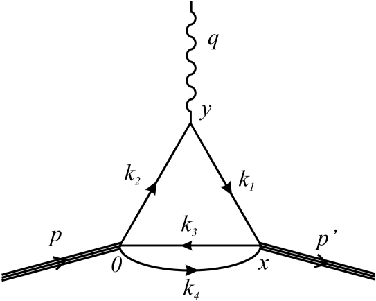
Figure 1:

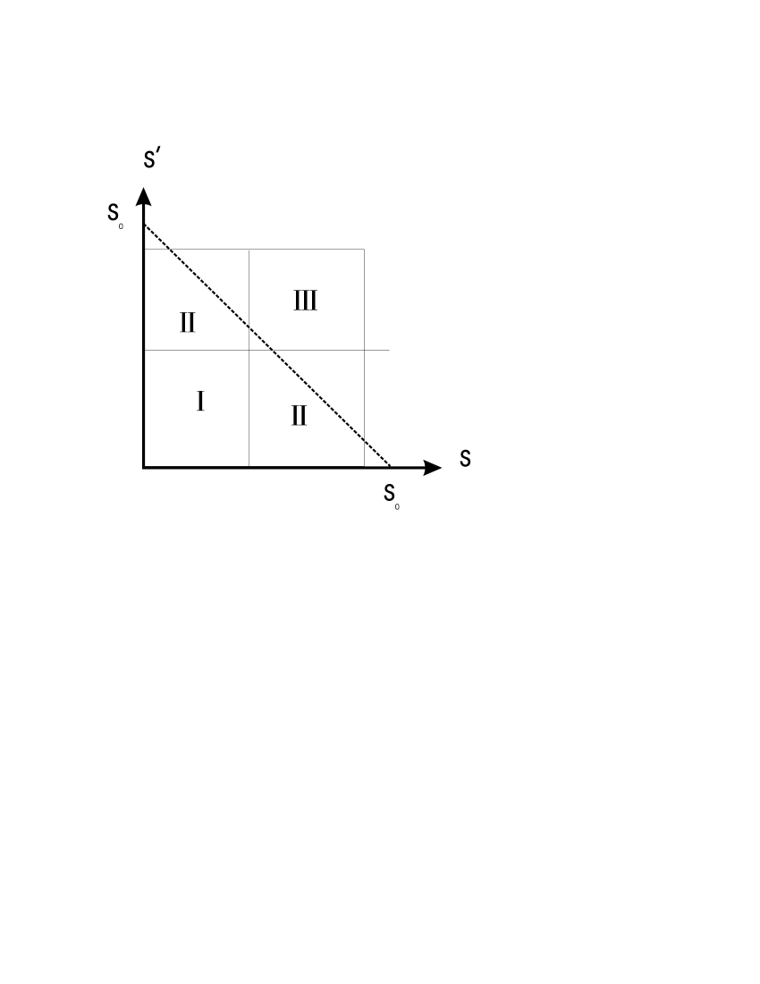
Figure 2:

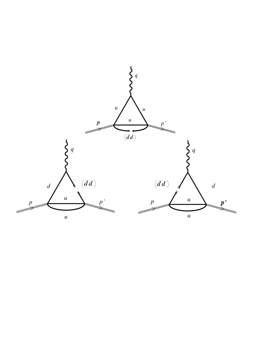
Figure 3:

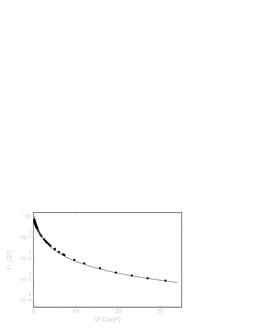
Figure 4:

Figure 5:

References

• [1] For a review see e.g. V.L. Chernyak, I.R. Zhitnitsky, Phys. Rep. 112 (1984) 173.
• [2] V.M. Braun et al., Phys. Rev. D 65 (2002) 074011; A. Lenz et al., hep-ph/0311082.
• [3] For a recent review see e.g. P. Colangelo, A. Khodjamirian, in ”At the frontiers of particle physics, Handbook of QCD, Vol. 3, 1495, M.A. Shifman, ed., (World Scientific, Singapore, 2001).
• [4] For a review see e.g. L.J. Reinders, H. Rubinstein, S. Yazaki, Phys. Rep. 127 (1985) 1.
• [5] C.A. Dominguez, M. Loewe, Z. Phys. C 58 (1993) 273.
• [6] B.L. Ioffe, Nucl. Phys. B 188 (1981) 817; Erratum: B 191 (1981) 591.
• [7] C.A. Dominguez, M. Loewe, J.S. Rozowsky, Phys. Lett. B 335 (1994) 506.
• [8] J. Arrington, Phys. Rev. C 68 (2003) 034325; ibid C 69 (2004) 022201.
• [9] E.J. Brash, A. Kozlov, Sh. Li, G.M. Huber, Phys. Rev. C 65 (2002) 051001.
• [10] G. Warren et al., Phys. Rev. Lett. 92 (2004) 042301; J. Bermuth et al., Phys. Lett. B 564 (2003) 199; M. Ostrick et al., Phys. Rev. Lett. 83 (1999) 276; J. Becker et al., Eur. Phys. J. A 6 (1999) 329; D. Rohe et al., Phys. Rev. Lett. 83 (1999) 4257; H. Zhu et al., Phys. Rev. Lett. 87 (2001) 081801; I. Passchier et al., Phys. Rev. Lett. 82 (1999) 4988; C. Herber et al., Eur. Phys. J. A 5 (1999) 131; J. Becker et al., Eur. Phys. J. A 6 (1999) 329; R. Madey et al., Phys. Rev. Lett. 91 (2003) 122002; J. Golak et al., Phys. Rev. C 63 (2001) 034006.