$J/\psi$ couplings to charmed resonances and to $\pi$

A. Deandrea^a, G. Nardulli^b,c and A. D. Polosa^d
aInstitut de Physique Nucléaire, Université de Lyon I
4 rue E. Fermi, F-69622 Villeurbanne Cedex, France
^bDipartimento di Fisica, Università di Bari, I-70124 Bari, Italia
^cI.N.F.N., Sezione di Bari, I-70124 Bari, Italia
^d CERN - Theory Division, CH-1211 Geneva 23, Switzerland

Abstract
We present an evaluation of the strong couplings $JD^{(*)}D^{(*)}$ and $JD^{(*)}D^{(*)}\pi$ by an effective field theory of quarks and mesons. These couplings are necessary to calculate $\pi+J/\psi\to D^{(*)}+\bar{D}^{(*)}$ cross sections, an important background to the $J/\psi$ suppression signal in the quark-gluon plasma. We write down the general effective Lagrangian and compute the relevant couplings in the soft pion limit and beyond.

PACS: 13.25.Gv 12.38.Lg
BARI-TH 459/03
CERN-TH/2003-45

Abstract

We present an evaluation of the strong couplings $JD^{(*)}D^{(*)}$ and $JD^{(*)}D^{(*)}\pi$ by an effective field theory of quarks and mesons. These couplings are necessary to calculate $\pi+J/\psi\to D^{(*)}+\bar{D}^{(*)}$ cross sections, an important background to the $J/\psi$ suppression signal in the quark-gluon plasma. We write down the general effective Lagrangian and compute the relevant couplings in the soft pion limit and beyond.

I Introduction

This paper is devoted to the study of the strong couplings of $J/\psi$, low mass charmed mesons and pions. The interest of this study stems from the possibility that $J/\psi$ absorption processes of the following type

$$\pi+J/\psi\to D^{(*)}+\bar{D}^{(*)}$$ (1)

play an important role in the relativistic heavy ion scattering. Since a decrease of the $J/\psi$ production might signal the formation of Quark Gluon Plasma (QGP) in a heavy ion collision, it is useful to have reliable estimates of the cross sections for the processes (1) that provide an alternative way to reduce the $J/\psi$ production rate. Previous studies of these effects can be found in cina1 ; c0 ; Deandrea:2002kj . The relevant couplings needed to compute (1) are depicted in Fig. 1.

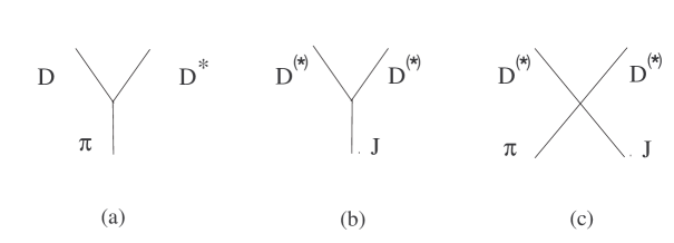
Figure 1: Couplings involved in the tree level calculations of the processes (1).

Besides the ${DD^{*}\pi}$ coupling, see Fig. 1a, whose coupling constant $g_{D^{*}D\pi}$ has been theoretically estimated theor , report and experimentally investigated exp , to compute the amplitudes (1) one would need also the $JD^{(*)}D^{(*)}$, see Fig. 1b, and the $J\,D^{(*)}D^{(*)}\pi$ couplings, see Fig. 1c. In an effective Lagrangian approach the latter couplings provide direct four-body interactions, while the former enter the amplitude via tree diagrams with the exchange of a charmed particle $D^{(*)}$ in the $t-$channel. These couplings have been estimated by different methods, that are, in our opinion, unsatisfactory. For example the use of the $SU_{4}$ symmetry puts on the same footing the heavy quark $c$ and the light quarks, which is at odds with the results obtained within the Heavy Quark Effective Theory (HQET), where the opposite approximation $m_{c}\gg\Lambda_{QCD}$ is used (for a short review of HQET see report ). Similarly, the rather common approach based on the Vector Meson Dominance (VMD) should be considered critically, given the large extrapolation $p^{2}=0\to m_{J/\psi}^{2}$ that is involved. A different evaluation, based on QCD Sum Rules can be found in qcdsr and presents the typical theoretical uncertainties of this method. In this note we will use a different approach, based on the Constituent Quark Meson (CQM) model nc ,nc1 , which takes into account explicitly the HQET symmetries. We gave a preliminary report of the present study in Deandrea:2002kj where we presented the results for some of the couplings (1). Here we complete the analysis and compare our results with the existing literature.

II Constituent Quark Meson model

The CQM model is a quark-meson model arising from an extension of Ref. Ebert:1994tv to exploit fully HQET and chiral symmetries in the interactions of heavy and light mesons. A survey of these methods can be found in nc ,nc1 . Here we limit to those aspects of the model that are relevant for the interactions of $J/\psi$, low mass charmed mesons and pions. The model is an effective field theory whose effective fields are light and heavy quarks as well as light and heavy mesons. The Feynman rules for the model are explicitly written down in nc , nc1 . The transition amplitudes containing light/heavy mesons in the initial and final states as well as the couplings of the heavy mesons to hadronic currents are computable via quark loop diagrams where mesons enter as external legs. The model is relativistic and incorporates, besides the heavy quark symmetries, also the chiral symmetry of the light quark sector.

To show an example of the calculation in the CQM model we consider the Isgur-Wise (IW) function defined e.g. by

$$\langle D(p^{\prime})|\bar{c}\gamma^{\mu}c|D(p)\rangle=m_{D}\xi(\omega)(v+v^{\prime})^{\mu}$$ (2)

where $p^{\mu}=m_{D}v^{\mu}$, $p^{\prime\,\mu}=m_{D}v^{\prime\,\mu}$ and $\omega=v\cdot v^{\prime}$. We note that the Isgur-Wise function obeys the normalization condition $\xi(1)=1$, arising from the flavor symmetry of the HQET. The explicit definition of the Isgur-Wise form factor is:

$$\langle H(v^{\prime})|\bar{c}\gamma_{\mu}c|H(v)\rangle=-\xi(\omega){\rm Tr}\left(\bar{H}\gamma_{\mu}H\right)\ .$$ (3)

Here $H$ is the multiplet containing both the $D$ and the $D^{*}$ mesons report :

$$H=\frac{1+\gamma\cdot v}{2}(-P_{5}\gamma_{5}+\gamma\cdot P)\ ,$$ (4)

and $P_{5},\,P^{\mu}$ are annihilation operators for the charmed mesons. One gets

$$\xi(\omega)(v+v^{\prime})^{\mu}=Z_{H}\frac{3i}{16\pi^{4}}\int d^{4}\ell\frac{{\rm Tr}\left[(\gamma\cdot\ell+m)\gamma_{5}(1+\gamma\cdot v^{\prime})\gamma_{\mu}(1+\gamma\cdot v)\gamma_{5}\right]}{4(\ell^{2}-m^{2})(v\cdot\ell+\Delta_{H})(v^{\prime}\cdot\ell-\Delta_{H})}\ ,$$ (5)

where $v$ and $v^{\prime}$ are the $4-$velocities of the two heavy quarks that are equal, in the infinite quark mass limit, to the hadron velocities,

$$\frac{1+\gamma\cdot v}{2(v\cdot\ell+\Delta_{H})}$$ (6)

is the heavy quark propagator of the HQET, and $\Delta_{H}=m_{D}-m_{c}=v\cdot k$ in the limit $m_{c}\to\infty$; $k$ is the meson residual momentum, defined by $p^{\mu}=m_{c}v^{\mu}+k^{\mu}$. The numerical value of $\Delta_{H}$ is in the range $0.3-0.5$ GeV nc . If we consider a $D^{*}$ meson instead of a $D$, a factor $-\gamma_{5}$ must be substituted by $\gamma\cdot\epsilon$, $\epsilon$ being the polarization of $D^{*}$. The constant $Z_{H}$ is the heavy meson field wavefunction renormalization constant giving the strength of the quark-meson coupling (more precisely the coupling is $\sqrt{Z_{H}m_{D}}$). $Z_{H}$ is computed and tabulated in nc . One gets for the IW function:

$$\xi(\omega)=Z_{H}\left[\frac{2}{1+\omega}I_{3}(\Delta_{H})+\left(m+\frac{2\Delta_{H}}{1+\omega}I_{5}(\Delta_{H},\Delta_{H},\omega)\right)\right]\ ,$$ (7)

where the $I_{i}$ integrals are given by:

$$I_{3}(\Delta) = -\frac{iN_{c}}{16\pi^{4}}\int^{\mathrm{reg}}\frac{d^{4}k}{(k^{2}-m^{2})(v\cdot k+\Delta+i\epsilon)}$$ (8)

$$= {N_{c}\over{16\,{{\pi}^{{3/2}}}}}\int_{1/{{\Lambda}^{2}}}^{1/{{\mu}^{2}}}{ds\over{s^{3/2}}}\;e^{-s({m^{2}}-{{\Delta}^{2}})}\;\left(1+{\mathrm{erf}}(\Delta\sqrt{s})\right)$$

$$I_{5}(\Delta_{1},\Delta_{2},\omega) = \frac{iN_{c}}{16\pi^{4}}\int^{\mathrm{reg}}\frac{d^{4}k}{(k^{2}-m^{2})(v\cdot k+\Delta_{1}+i\epsilon)(v^{\prime}\cdot k+\Delta_{2}+i\epsilon)}$$ (9)

$$= \int_{0}^{1}dx\frac{1}{1+2x^{2}(1-\omega)+2x(\omega-1)}\times$$

$$\Big{[}\frac{6}{16\pi^{3/2}}\int_{1/\Lambda^{2}}^{1/\mu^{2}}ds~{}\sigma\;e^{-s(m^{2}-\sigma^{2})}\;s^{-1/2}\;(1+{\mathrm{erf}}(\sigma\sqrt{s}))+$$

$$\frac{6}{16\pi^{2}}\int_{1/\Lambda^{2}}^{1/\mu^{2}}ds\;e^{-s\sigma^{2}}\;s^{-1}\Big{]},$$

where

$$\sigma(x,\Delta_{1},\Delta_{2},\omega)={{{\Delta_{1}}\,\left(1-x\right)+{\Delta_{2}}\,x}\over{{\sqrt{1+2\,\left(\omega-1\right)\,x+2\,\left(1-\omega\right)\,{x^{2}}}}}}.$$ (10)

The ultraviolet cutoff $\Lambda$, the infrared cutoff $\mu$ and the light constituent mass $m$ are fixed in the model nc to be $\Lambda=1.25$ GeV, $\mu=0.3$ GeV and $m=0.3$ GeV. Other integrals to be used later are

$$I_{2} = -\frac{iN_{c}}{16\pi^{4}}\int^{\mathrm{reg}}\frac{d^{4}k}{(k^{2}-m^{2})^{2}}={N_{c}\over{16\,{{\pi}^{{2}}}}}\Gamma\left(0,\frac{m^{2}}{\Lambda^{2}},\frac{m^{2}}{\mu^{2}}\right)$$ (11)

$$I_{4}(\Delta) = \frac{iN_{c}}{16\pi^{4}}\int^{\mathrm{reg}}\frac{d^{4}k}{(k^{2}-m^{2})^{2}(v\cdot k+\Delta+i\epsilon)}$$ (12)

$$= \frac{N_{c}}{16\pi^{3/2}}\int_{1/\Lambda^{2}}^{1/\mu^{2}}\frac{ds}{s^{1/2}}\;e^{-s(m^{2}-\Delta^{2})}\;[1+{\mathrm{erf}}(\Delta\sqrt{s})]$$

The calculation of the $g_{D^{*}D\pi}$ coupling constant for the matrix element

$$\langle\pi^{+}(q)D^{0}(p)|D^{*+}(p^{\prime},\epsilon)\rangle=ig_{D^{*}D\pi}\epsilon\cdot q$$ (13)

in the CQM proceeds along similar lines and can be found in nc . We reproduce for reference’s sake since it is an important element of the amplitudes (1). In the soft pion limit (spl) one gets nc :

$$g_{D^{*}D\pi}^{spl}=13\pm 1~{}.$$ (14)

The experimental situation is as follows: CLEO results exp give $g=0.59\pm 0.07\pm 0.01$ where $g$ is related to the constant in eq. (14) by $g_{D^{*}D\pi}^{spl}=2m_{D}g/f_{\pi}$ ($f_{\pi}\approx 130$ MeV); on the other hand, in general, QCD sum rules predict smaller values, see for a review report .

III $JD^{(*)}D^{(*)}$ couplings

The calculation of the Isgur-Wise we have described above is a crucial ingredient to the computation of the $JD^{(*)}D^{(*)}$ vertexes of Fig. 1b. It corresponds to the evaluation of the l.h.s. of Fig. 2, while, via a VMD ansatz, the r.h.s. gives the desired coupling. Concerning the use of the VMD for the charm system one has to note that it is not based on the hypothesis that all higher order resonances give contributions smaller than the J/$\psi$, but on the fact that the higher states give contributions of alternating sign that tend to cancel. This sign difference follows from an evaluation via the saddle point method of the WKB approximation altern .

Figure 2: The Vector Meson Dominance equation giving the coupling of $J/\psi$ with $D,D^{*}$ in terms of the Isgur-Wise function $\xi$. The function $\xi$ on the l.h.s. is computed by a diagram with a quark loop. The coupling of each $D^{(*)}$ meson to quarks is given by $\sqrt{Z_{H}m_{D}}$.

The Isgur-Wise function can be computed for any value of $\omega$ and not only in the region $\omega>1$, which is experimentally accessible $via$ the semileptonic $B\to D^{(*)}$ decays; $\omega$ is related to the meson momenta by

$$\omega=\frac{p_{1}^{2}+p_{2}^{2}-p^{2}}{2\sqrt{p_{1}^{2}p_{2}^{2}}}\,,$$ (15)

where $p_{1},\,p_{2}=$ momenta of the two $D$ resonances.

Let us now consider the r.h.s. of the equation depicted in Fig. 2. For the coupling of $J/\psi$ to the current we use the matrix element

$$\langle 0|\bar{c}\gamma^{\mu}c|J(q,\eta)\rangle=f_{J}m_{J}\epsilon^{\mu}$$ (16)

with $f_{J}=0.405\pm 0.014$ GeV. As to the strong couplings $JD^{(*)}D^{(*)}$, the model in Fig. 2 gives the following effective Lagrangians

$${\cal L}_{JDD} = ig_{JDD}\left(\bar{D}{\stackrel{{\scriptstyle\leftrightarrow}}{{\partial}}}_{\nu}D\right)J^{\nu}\ ,$$ (17)

$${\cal L}_{JDD^{*}} = ig_{JDD^{*}}\epsilon^{\mu\nu\alpha\beta}J_{\mu}\partial_{\nu}\bar{D}\partial_{\beta}D^{*}_{\alpha}\ ,$$ (18)

$${\cal L}_{JD^{*}D^{*}} = ig_{JD^{*}D^{*}}\Big{[}\bar{D}^{*\mu}\left({\partial}_{\mu}D^{*}_{\nu}\right)J^{\nu}-{D}^{*\mu}\left({\partial}_{\mu}\bar{D}^{*}_{\nu}\right)J^{\nu}$$ (20)

$$- \left(\bar{D}^{*\mu}{\stackrel{{\scriptstyle\leftrightarrow}}{{\partial}}}_{\nu}D^{*}_{\mu}\right)J^{\nu}\Big{]}\ .$$ (21)

Here $D^{(*)}\bar{D}^{(*)}$ can be any of the pairs $D^{0(*)}\bar{D}^{0(*)}$, $D^{+(*)}D^{-(*)}$ or $D_{s}^{(*)}\bar{D}_{s}^{(*)}$ (neglecting $SU_{3}$ breaking effects). As a consequence of the spin symmetry of the HQET we find:

$$g_{JD^{*}D^{*}}=g_{JDD}\,,~{}~{}~{}~{}~{}~{}~{}~{}~{}~{}g_{JDD^{*}}=\frac{g_{JDD}}{m_{D}}\ ,$$ (22)

while the VMD ansatz gives:

$$g_{JDD}(p_{1}^{2},\,p_{2}^{2},\,p^{2})=\frac{m^{2}_{J}-p^{2}}{f_{J}m_{J}}\xi(\omega)\ .$$ (23)

Since $g_{JDD}$ has no zeros, eq. (23) shows that $\xi$ has a pole at $p^{2}=m^{2}_{J}$, which is what one expects on the basis of dispersion relations arguments. The CQM evaluation of $\xi$ does show a strong peak for $p^{2}\approx(2m_{c})^{2}$, even though, due to $\displaystyle{\cal O}\,\left({1}/{m_{c}}\right)$ effects, the location of the singularity is not exactly at $p^{2}=m^{2}_{J}$.

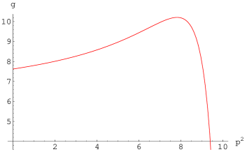
Figure 3: The $p^{2}$ dependence of $g=g_{JDD}(m_{D}^{2},\,m^{2}_{D},\,p^{2})$, showing the almost complete cancellation between the pole of the Isgur-Wise function and the kinematical zero. Units are GeV² for $p^{2}$.

This is shown in Fig. 3 where we plot $g_{JDD}(p_{1}^{2},\,p_{2}^{2},\,p^{2})$ for on shell $D$ mesons, as a function of $p^{2}$ (the plot is obtained for $\Delta_{H}=0.4$ GeV and $Z_{H}=2.36~{}$GeV^-1). For $p^{2}$ in the range $(0,4)$ GeV², $g_{JDD}$ is almost flat, with a value

$$g_{JDD}=8.0\pm 0.5\ .$$ (24)

For larger values of $p^{2}$ the method is unreliable due to the above-mentioned incomplete cancellation between the kinematical zero and the pole. Therefore, we extrapolate the smooth behavior of $g_{JDD}$ in the small $p^{2}$ region up to $p^{2}=m^{2}_{J}$ and assume the validity of the result (24) also for on-shell $J/\psi$ mesons. On the other hand in the $p_{1}^{2},p^{2}_{2}$ variables we find a behavior compatible with that produced by a smooth form factor. Also the result from Ref. cina1 in the Table, is based on a VMD assumption; a previous determination based on the same assumption is matinyan , with similar results ($g_{JDD}=7.7$).

In Table 1 we compare our results with those of other authors. We observe that our results for $g_{JDD}$ and $g_{JDD^{*}}$ agree with the outcomes of Ref. cina2 and with the QCD sum rule analysis of qcdsr ; in particular the smooth behavior of the form factor found in qcdsr for $g_{JDD}$ agrees with our result. This is not surprising, as cina2 uses a VMD model as well.

As for the QCD sum rules calculation, it involves a perturbative part and a non perturbative contribution, which is however suppressed. The perturbative term has its counterpart in CQM in the loop calculation of Fig. 2 and the overall normalization should agree as a consequence of the Luke’s theorem. On the other hand we differ from Ref. cina1 for a sign and from haglin both in sign and in magnitude. The sign difference may be due to an overall phase in the $J/\Psi$ wavefunction. It is however of no effect in the computation of the $J/\Psi$ absorption cross section, which is the main application of the present calculation. Finally Ref. cina2 obtains a value for $g_{JDD^{*}}$ using results from the decay $J/\psi\to\rho\pi$. This seems to us too strong an assumption due to the fact that $J/\psi\to\rho\pi$ could proceed via gluonic decay of the $J/\psi$, which is not the case for $J/\psi\to DD^{*}$.

Coupling	Our work	Ref. cina1	Ref. haglin	Ref. cina2	Ref. qcdsr
$g_{JDD}$	$8.0\pm 0.5$	-7.64	$-4.93$	7.71	7.36
$g_{JDD^{*}}$(GeV-1)	$4.05\pm 0.25$	-		$8.02\pm 0.62$	-
$g_{JD^{*}D^{*}}$	$8.0\pm 0.5$	-7.64	$-4.93$	7.71	-

Table 1. Comparison of theoretical results for the couplings $g_{JDD}$, $g_{JDD^{*}}$ and $g_{JD^{*}D^{*}}$. Ref. cina1 and Ref. cina2 use a VMD model similar to the one used in the present paper for the couplings $g_{JDD}$, $g_{JD^{*}D^{*}}$. For $g_{JDD^{*}}$ Ref. cina2 uses VMD together with data from relativistic quark model Colangelo:1994jc to get the coupling of a hadronic current to $D$ and $D^{*}$. Ref. haglin uses a chiral model to compute the coupling constants $g_{JDD}$ and $g_{JD^{*}D^{*}}$. The coupling $g_{JDD^{*}}$ is not included in Ref. cina1 . Ref. qcdsr is based on QCD sum rules; the result we report for $g_{JDD}$ is computed at the same value $p^{2}=2$ GeV² as in our work.

IV $JD^{(*)}D^{(*)}\pi$ couplings

Let us now consider the $JD^{(*)}D^{(*)}\pi$ couplings of Fig. 1c. We write the effective Lagrangians for the $J\pi^{+}D^{-}D^{0}$ coupling (other couplings can be obtained by use of symmetries):

$${\cal L}_{JDD\pi} = \frac{g_{0}}{m_{D}}\epsilon^{\mu\nu\alpha\beta}J_{\mu}(\partial_{\nu}\pi)\partial_{\alpha}D\partial_{\beta}\bar{D}\,,$$ (25)

$${\cal L}_{J{\bar{D}}^{*}D\pi} = -\,J_{\mu}(\partial_{\nu}\pi)\Big{\{}g_{1}\left[g^{\mu\nu}{\bar{D}}^{*}_{\lambda}\partial^{\lambda}\,D+2\,D\,\partial^{\mu}{\bar{D}}^{*\nu}\right]-g_{2}\left[{\bar{D}}^{*\mu}\partial^{\nu}+D\partial^{\nu}{\bar{D}}^{*\mu}\right]$$ (26)

$$+ \frac{g_{3}}{m_{D}^{2}}\left[\left(\partial^{\nu}{\bar{D}}^{*\lambda}\right)\partial^{\mu}\partial_{\lambda}D-\left(\partial^{\nu}\partial_{\lambda}D\right)\partial^{\mu}{\bar{D}}^{*\lambda}\right]\Big{\}}~{}+~{}h.c.\,,$$ (27)

$${\cal L}_{J{\bar{D}}^{*}D^{*}\pi} = m_{D}J^{\mu}(\partial^{\nu}\pi)\Big{\{}g_{4}\,\epsilon_{\mu\nu\rho\lambda}{D}^{*\rho}{\bar{D}}^{*\lambda}+\frac{g_{5}}{m_{D}^{2}}\epsilon_{\mu\alpha\beta\lambda}\left(\partial^{\alpha}\partial_{\nu}{D}^{*\beta}\right){\bar{D}}^{*\lambda}$$ (28)

$$- \frac{g_{6}}{m^{2}_{D}}\epsilon_{\mu\alpha\beta\lambda}\left(\partial_{\nu}{D}^{*\alpha}\right)\partial^{\lambda}{\bar{D}}^{*\beta}$$ (29)

$$+ \frac{g_{7}}{m^{2}_{D}}\Big{[}\epsilon_{\mu\alpha\nu\beta}\left(\partial_{\lambda}\partial^{\alpha}{D}^{*\beta}\right){\bar{D}}^{*\lambda}-2\,\epsilon_{\mu\alpha\lambda\beta}\left(\partial^{\alpha}{D}^{*\lambda}\right)\partial^{\beta}{\bar{D}}^{*\nu}$$ (30)

$$+ 2\,\epsilon_{\mu\nu\alpha\beta}{D}^{*\lambda}\partial_{\lambda}\partial^{\alpha}{\bar{D}}^{*\beta}+\epsilon_{\alpha\nu\beta\lambda}\left(\partial^{\alpha}{D}^{*}_{\mu}\right)\partial^{\lambda}{\bar{D}}^{*\beta}$$ (31)

$$+ g_{\mu\nu}\epsilon_{\alpha\beta\rho\lambda}\left(\partial^{\alpha}{D}^{*\beta}\right)\partial^{\lambda}{\bar{D}}^{*\rho}-2\epsilon_{\nu\alpha\beta\lambda}{D}^{*\alpha}\partial^{\lambda}\partial_{\mu}{\bar{D}}^{*\beta}\Big{]}$$ (32)

$$+ \frac{g_{7}^{\prime}}{m^{2}_{D}}\,\epsilon_{\mu\alpha\beta\lambda}\left(\partial^{\alpha}{D}^{*}_{\nu}\right)\partial^{\lambda}{\bar{D}}^{*\beta}$$ (33)

$$+ \frac{g_{8}}{m^{2}_{D}}\,\epsilon_{\mu\alpha\beta\lambda}{D}^{*\alpha}\partial^{\lambda}\partial_{\nu}{\bar{D}}^{*\beta}+\frac{g_{9}}{m^{2}_{D}}\,\epsilon_{\mu\alpha\beta\lambda}\left(\partial^{\beta}{D}^{*\alpha}\right)\partial_{\nu}{\bar{D}}^{*\lambda}$$ (34)

$$+ \frac{g_{1}}{m^{2}_{D}}\,\epsilon_{\nu\alpha\beta\lambda}\left(\partial^{\alpha}\partial_{\mu}{D}^{*\beta}\right){\bar{D}}^{*\lambda}+\frac{g_{7}^{\prime\prime}}{m^{2}_{D}}\,\epsilon_{\nu\alpha\beta\lambda}\left(\partial^{\alpha}{D}^{*\beta}\right)\partial^{\lambda}{\bar{D}}^{*}_{\mu}$$ (35)

$$- \frac{g_{9}}{m^{4}_{D}}\,\left[\epsilon_{\mu\alpha\beta\lambda}\left(\partial^{\alpha}\partial_{\nu}{D}^{*\rho}\right)\partial^{\lambda}\partial_{\rho}{\bar{D}}^{*\beta}+\epsilon_{\alpha\rho\beta\lambda}\left(\partial^{\alpha}\partial_{\nu}{D}^{*\rho}\right)\partial^{\lambda}\partial_{\mu}{\bar{D}}^{*\beta}\right]$$ (36)

$$+ \frac{g_{9}^{\prime}}{m^{4}_{D}}\left[\epsilon_{\mu\alpha\beta\lambda}\left(\partial^{\alpha}{D}^{*\rho}\right)\partial_{\rho}\partial_{\nu}\partial^{\lambda}{\bar{D}}^{*\beta}+\epsilon_{\alpha\rho\beta\lambda}\left(\partial^{\alpha}{D}^{*\rho}\right)\partial^{\lambda}\partial_{\mu}\partial_{\nu}{\bar{D}}^{*\beta}\right]\Big{\}}.$$ (37)

While in these formulae 13 coupling constants appear, the number of the independent couplings is only 5. As a matter of fact they can be written in terms of the independent couplings $A_{1}\,,A_{2}\,,A_{4}\,,B\,,K$ defined by the formulae

$$\frac{3i}{16\pi^{4}}\int\,d^{4}\ell\,\frac{\ell^{\alpha}\ell^{\beta}}{(\ell^{2}-m^{2})[(\ell+q)^{2}-m^{2}](v\cdot\ell+\Delta)(v^{\prime}\cdot\ell+\Delta)}=A_{1}g^{\alpha\beta}+$$ (38)

(39)

$$~{}~{}~{}~{}~{}~{}~{}~{}~{}~{}~{}~{}~{}~{}~{}~{}~{}~{}~{}~{}~{}~{}~{}~{}~{}~{}~{}~{}~{}~{}~{}~{}~{}~{}~{}~{}~{}~{}~{}~{}+A_{2}\left(v^{\alpha}v^{\beta}+v^{\prime\alpha}v^{\prime\beta}\right)+A_{4}\left(v^{\prime\alpha}v^{\beta}+v^{\alpha}v^{\prime\beta}\right),$$ (40)

(41)

$$\frac{3i}{16\pi^{4}}\int\,d^{4}\ell\,\frac{\ell^{\alpha}}{(\ell^{2}-m^{2})[(\ell+q)^{2}-m^{2}](v\cdot\ell+\Delta)(v^{\prime}\cdot\ell+\Delta)}=B\,\left(v^{\alpha}+v^{\prime\beta}\right),$$ (42)

$$\frac{3i}{16\pi^{4}}\int\,d^{4}\ell\,\frac{1}{(\ell^{2}-m^{2})[(\ell+q)^{2}-m^{2}](v\cdot\ell+\Delta)(v^{\prime}\cdot\ell+\Delta)}=K\,.$$ (43)

The dependence of the $g_{k}$ on these couplings is in Table 2.

Coupling	CQM formula
$g_{0}$	$\beta\,[(4m+2\Delta_{H})B-m^{2}K]$
$g_{1}$	$\beta\,[2A_{1}+2A_{2}+2\omega A_{4}-4mB+m^{2}K]$
$g_{2}$	$\beta\,[2A_{1}+2\omega A_{2}+2A_{4}-2(1+\omega)mB+m^{2}K]$
$g_{3}$	$2\beta\,[A_{2}-A_{4}-mB]$
$g_{4}$	$\beta\,[2A_{1}+2A_{2}+2\omega A_{4}-(1+\omega)mB+m^{2}K]$
$g_{5}$	$\beta\,[2A_{2}-mB]$
$g_{6}$	$\beta\,[2A_{1}+2A_{4}-mB+m^{2}K]$
$g_{7}$	$\beta mB$
$g_{7}^{\prime}$	$g_{1}+2g_{7}$
$g_{7}^{\prime\prime}$	$g_{1}+g_{7}$
$g_{8}$	$2\beta[(1-\omega)A_{2}-A_{4}]$
$g_{9}$	$2\,\beta\,A_{4}$
$g_{9}^{\prime}$	$g_{5}+g_{7}$

Table 2. Relations between the coupling constants $g_{k}$ and the constants $A_{1}$, $A_{2}$, $A_{4}$, $B$ and $K$. Units are GeV^-2; $\omega$ is defined in eq.(15), with $p^{2}_{1}=p^{2}_{2}=m^{2}_{D}$ and $p^{2}=2$ GeV² for $g_{0}\,,g_{1}\,,g_{4}\,,g_{7}$ and $p^{2}=5$ GeV² for $g_{2}\,,g_{3}\,,g_{5}\,,g_{8}\,,g_{9}$.In this table

$$\beta=\frac{m_{J}^{2}-p^{2}}{f_{\pi}f_{J}m_{J}}\,Z_{H}\,,$$ (44)

and explicit formulae for $A_{1}\,,A_{2}\,,A_{4}\,,B\,,K$ can be found in Section V. These results have been obtained by a VMD ansatz similar to Fig. 2, but now the l.h.s is modified by the insertion of a soft pion on the light quark line (with a coupling $q_{\pi}^{\mu}/f_{\pi}\gamma_{\mu}\gamma_{5}$). Let us discuss in some detail one of these couplings, $g_{0}$. The numerical results for on-shell $D$ mesons, in the soft pion limit as a function of the $J/\psi$ virtuality show a behavior similar to that of Fig. 3. By the same arguments used to determine $g_{JDD}$ in Fig. 3 we choose $p^{2}=2$ GeV² and we get

$$\frac{g_{0}}{m_{D}}=125\pm 15~{}{\rm GeV}^{-3}~{}~{}~{}~{}~{}({\rm soft~{}pion~{}limit})\ .$$ (45)

In order to include hard pion effects we write the general formula

$$g_{k}(|\vec{q}_{\pi}|)=g_{k}(0)\,f_{k}(|\vec{q}_{\pi}|),$$ (46)

where $f_{k}(|\vec{q}_{\pi}|)$ is a form factor. We will discuss it in the next section. For the time being we report the values of all the coupling constants in the soft pion limit in Table 3.

Coupling	Results (GeV-2)	Coupling	Results (GeV-2)
$g_{0}(0)$	$+234\pm 45$	$g_{5}(0)$	$-274\pm 49$
$g_{1}(0)$	$-235\pm 38$	$g_{6}(0)$	$+104\pm 16$
$g_{2}(0)$	$-126\pm 19$	$g_{7}(0)$	$+30\pm 5$
$g_{3}(0)$	$-252\pm 38$	$g_{8}(0)$	$-106\pm 22$
$g_{4}(0)$	$-165\pm 25$	$g_{9}(0)$	$-63\pm 37$

Table 3. Results for the coupling constants $g_{j}(|\vec{q}_{\pi}|)$ in the soft pion limit $q_{\pi}\to 0$.

In computing this table we have adopted a criterion of stability in $p^{2}$ analogous to the one used for $g_{0}$. For $g_{0}\,,g_{1}\,,g_{4}\,,g_{7}$ we find stability at the $J/\psi$ virtuality $p^{2}=2$ GeV². For $g_{2}\,,g_{3}\,,g_{5}\,,g_{8}\,,g_{9}$ we find stability at $p^{2}=5$ GeV². The technical reason for this difference is that, in the latter case, the equations do not determine the five constants for $p^{2}\approx 0$; therefore the stability region lies around the center of the $p^{2}$ interval $(0,m_{J}^{2})$. For $g_{6}$ we do not find stability and we derive it by consistency equations derived from Table 2. To the error arising from the stability analysis we have added a further theoretical uncertainty of $\pm 15\%$ in quadrature.

An attempt to compute quadrilinear couplings via $SU_{4}$ symmetry relations can be found in cina1 and in cina2 . For example, the result for $g_{0}$ obtained in cina2 is 30 GeV^-2. The difference with Table 3 is due to the large $SU_{4}$ violations of our model $(m_{c}>>m_{u},m_{s})$.

V Form factors

The coupling constants $g_{j}$ can be expressed in terms of the constants $A_{j}$, $B$ and $K$ using the results of Table 2. These constants, for $|\vec{q}_{\pi}|\neq 0$, are expressed in terms of parametric integrals $I_{j}$ as follows:

$$A_{1} = \frac{C_{1}(1-\omega^{2})-2C_{3}+2C_{2}\omega}{2(1-\omega^{2})}\ ,$$ (47)

$$A_{2} = \frac{C_{1}(\omega^{2}-1)-6C_{2}\omega+2C_{3}(2+\omega^{2})}{2(\omega^{2}-1)^{2}}\ ,$$ (48)

$$A_{4} = \frac{C_{2}(2+4\omega^{2})+\omega(C_{1}(1-\omega^{2})-6C_{3})}{2(\omega^{2}-1)^{2}}\ ,$$ (49)

$$B(q_{\pi}) = \frac{1}{1+\omega}\int_{0}^{1}dx[I_{4}(\Delta^{\prime}(x,q_{\pi}))-\Delta(x,q_{\pi})K(x,q_{\pi})]\ ,$$ (50)

$$K(q_{\pi}) = \int_{0}^{1}dxK(x,q_{\pi}),$$ (51)

where

$$C_{1}(q_{\pi}) = \int_{0}^{1}dx[I_{5}(\Delta(x,q_{\pi}),\Delta^{\prime}(x,q_{\pi}),{\omega})+m^{2}K(x,q_{\pi})]\ ,$$ (52)

$$C_{2}(q_{\pi}) = -I_{2}-\int_{0}^{1}dx[\Delta^{\prime}(x,q_{\pi})I_{4}(\Delta^{\prime}(x,q_{\pi}))+\Delta(x,q_{\pi})I_{4}(\Delta(x,q_{\pi}))$$ (53)

$$- \Delta(x,q_{\pi})\Delta^{\prime}(x,q_{\pi})K(x,q_{\pi})]\ ,$$ (54)

$$C_{3}(q_{\pi}) = -\omega I_{2}-\int_{0}^{1}dx[(\Delta(x,q_{\pi})+{\omega}\Delta^{\prime}(x,q_{\pi}))I_{4}(\Delta^{\prime}(x,q_{\pi}))\Delta^{2}(x,q_{\pi})K(x,q_{\pi})]\ ,$$ (55)

$$K(x,q_{\pi}) = \frac{\partial}{\partial m^{2}}I_{5}(\Delta(x,q_{\pi}),\Delta^{\prime}(x,q_{\pi}),{\omega}),$$ (56)

and we have defined

$$\Delta(x,q_{\pi}) = \Delta-q_{\pi}x\ ,$$ (57)

$$\Delta^{\prime}(x,q_{\pi}) = \Delta-q_{\pi}x{\omega}\ .$$ (58)

To compute the integrals we have applied the Feynman trick with the shift $\ell+qx\to\ell^{\prime}$ where the pion momentum is $q_{\mu}=(q_{\pi},0,0,q_{\pi})$. $\omega$ is computed by eq. (15) with the appropriate value of $p^{2}$, according to the discussion above. Moreover we have used the approximation:

$$v^{\prime\mu}=\omega\,v^{\mu}\ ,$$ (59)

which has the correct normalization at $\omega=1$ and also satisfies the constraint $\omega=v\cdot v^{\prime}$. Using (59) we assume that at least one of the two charmed resonances is off-shell, simplifying considerably the numerical computation. A numerical calculation of the integrals in these equations leads to a general fit of the form factors as follows:

$$f_{k}(|\vec{q}_{\pi}|)=\frac{1}{\displaystyle 1+\frac{|\vec{q}_{\pi}|}{m_{k}}}\ ,$$ (60)

with approximately the same value for all the form factors:

$$m_{k}=0.20\pm 0.05~{}~{}{\rm GeV}\ .$$ (61)

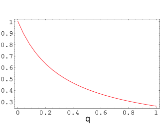
Figure 4: The dependence of $g(q)\equiv g_{D^{*}D\pi}(q)/g_{DD\pi}(0)$ on the pion momentum $q$.

It is useful to compute the corrections to the soft pion limit also for the $DD^{*}\pi$ coupling constants whose value for $q_{\pi}\to 0$ was computed in nc and reported in eq. (14). Using the same technique employed above we make the substitution

$$\frac{1}{(\ell^{2}-m^{2})^{2}}\to\frac{1}{(\ell^{2}-m^{2})[(\ell+q)^{2}-m^{2}]}$$ (62)

and compute the integrals appearing in eq. (63) of nc by the Feynman method as above. The result of this calculation is plotted in Fig. 4. The dependence can be fitted by a formula similar to eq. (60) with a mass $m_{\chi}=0.37$ GeV:

$$g_{D^{*}D\pi}(|\vec{q}_{\pi}|)=\frac{g_{D^{*}D\pi}^{spl}}{1+\frac{|\vec{q}_{\pi}|}{m_{\chi}}}\ .$$ (63)

It is useful to compare this result with that found in Ref. Isola:2001ar for the same quantity computed in a QCD inspired potential model. In that case one finds again a similar form factor with $m_{\chi}=0.20\pm 0.10$ GeV. These two determinations are sufficiently compatible and induce us to be confident that the method we have used to get the results (60) and (61) is reliable. It can be noted that considering a different extrapolation, i.e. in the pion virtuality $Q^{2}$, as in Ref. navarra2 , a smoother behavior is obtained, which should be relevant in the calculation of the $J/\Psi$ absorption cross section.

VI Conclusions

As discussed in falk , but see also report , the leading contributions to the current matrix element $\langle H(v^{\prime})\pi|\bar{c}\gamma^{\mu}c|H(v)\rangle$ in the soft pion limit (spl) are the pole diagrams. The technical reason is that, in the spl, the reducing action of a pion derivative in the matrix element is compensated in the polar diagrams by the effect of the denominator that vanishes in the combined limit $q_{\pi}\to 0,\,m_{c}\to\infty$. Let us now compare this result with the effective $JDD\pi$ coupling obtained by a polar diagram with an intermediate $D^{*}$ state. We get in this case

$$g_{0}^{polar}\approx\frac{g_{JDD^{*}}g_{D^{*}D\pi}m_{D}}{2q_{\pi}\cdot p_{D}}\ .$$ (64)

This expression dominates over the result (45) for pion momenta smaller than 100 MeV. If one restricts the model to the soft pion limit ($|\vec{q}_{\pi}|<100$ MeV), in spite of the rather large value of $g_{0}(0)$ the diagrams containing this coupling are suppressed, and one can expect a similar result also for the other couplings. However, to allow the production of a $D^{(*)}D^{(*)}$ pair by processes (1), one has to go beyond the spl, since the threshold for the charmed meson pair is $|\vec{q}_{\pi}|=700-1000~{}$ MeV. Our results show that in the CQM model this is indeed possible, by including computed form factors as in (60) and (63). Similar form factors were considered in cina1 , with a different motivation. Here we have shown that the CQM model not only allows their computation, but also gives the general expression for the trilinear and quartic couplings of $J/\psi$ to charmed mesons and pions. In spite of its model dependent character this seems to us an interesting result. Applications to the problem of the $J/\psi$ absorption in a nuclear medium will be considered elsewhere.

References

- (1) Z.W. Lin and C.M. Ko, Phys. Rev. C 62, 034903 (2000) [arXiv:nucl-th/9912046].
- (2) J. W. Qiu, J. P. Vary and X. F. Zhang, Phys. Rev. Lett. 88, 232301 (2002) [arXiv:hep-ph/9809442]; Y. s. Oh, T. s. Song, S. H. Lee and C. Y. Wong, [arXiv:nucl-th/0205065].
- (3) A. Deandrea, G. Nardulli and A. D. Polosa, in ’Workshop on Hard Probes in Heavy Ion Collisions at the LHC’ [arXiv:hep-ph/0211431].
- (4) P. Colangelo, F. De Fazio and G. Nardulli, Phys. Lett. B 334 (1994) 175 [arXiv:hep-ph/9406320]. P. Colangelo, G. Nardulli, A. Deandrea, N. Di Bartolomeo, R. Gatto and F. Feruglio, Phys. Lett. B 339, 151 (1994) [arXiv:hep-ph/9406295].
- (5) R. Casalbuoni, A. Deandrea, N. Di Bartolomeo, R. Gatto, F. Feruglio and G. Nardulli, Phys. Rept. 281, 145 (1997) [arXiv:hep-ph/9605342].
- (6) S. Ahmed et al. [CLEO Collaboration], Phys. Rev. Lett. 87, 251801 (2001) [arXiv:hep-ex/0108013].
- (7) R. D. Matheus, F. S. Navarra, M. Nielsen and R. Rodrigues da Silva, Phys. Lett. B 541, 265 (2002) [arXiv:hep-ph/0206198]; F. O. Duraes, S. H. Lee, F. S. Navarra and M. Nielsen, [arXiv:nucl-th/0210075].
- (8) A. Deandrea, N. Di Bartolomeo, R. Gatto, G. Nardulli and A.D. Polosa, Phys. Rev. D 58, 034004 (1998) [arXiv:hep-ph/9802308].
- (9) A.D. Polosa, Riv. Nuovo Cim. 23N11, 1 (2000) [arXiv:hep-ph/0004183].
- (10) D. Ebert, T. Feldmann, R. Friedrich and H. Reinhardt, Nucl. Phys. B 434, 619 (1995) [arXiv:hep-ph/9406220].
- (11) P. Cea and G. Nardulli, Phys. Rev. D 34 (1986) 1863.
- (12) S. G. Matinian and B. Muller, Phys. Rev. C 58, 2994 (1998) [arXiv:nucl-th/9806027].
- (13) Y. Oh, T. Song and S.H. Lee, Phys. Rev. C 63, 034901 (2001) [arXiv:nucl-th/0010064].
- (14) K. L. Haglin and C. Gale, Phys. Rev. C 63, 065201 (2001) [arXiv:nucl-th/0010017].
- (15) P. Colangelo, F. De Fazio and G. Nardulli, Phys. Lett. B 334, 175 (1994) [arXiv:hep-ph/9406320].
- (16) C. Isola, M. Ladisa, G. Nardulli, T. N. Pham and P. Santorelli, Phys. Rev. D 64, 014029 (2001) [arXiv:hep-ph/0101118].
- (17) F. S. Navarra, M. Nielsen, M. E. Bracco, M. Chiapparini and C. L. Schat, Phys. Lett. B 489, 319 (2000) [arXiv:hep-ph/0005026].
- (18) A. F. Falk, H. Georgi, B. Grinstein and M. B. Wise, Nucl. Phys. B 343, 1 (1990).