PCCF-RI-03-03

ADP-03-111/T549

Direct $\boldsymbol{CP}$ Violation In $\boldsymbol{B\rightarrow\pi^{+}\pi^{-}V}$ With $\boldsymbol{\rho^{0}-\omega}$ Mixing Effects: Phenomenological Approach

Z.J. Ajaltouni¹, O. Leitner^1,2, P. Perret¹, C. Rimbault¹,
A.W. Thomas²

¹ Laboratoire de Physique Corpusculaire de Clermont-Ferrand
IN2P3/CNRS Université Blaise Pascal
F-63177 Aubière Cedex France
² Department of Physics and Mathematical Physics and
Special Research Centre for the Subatomic Structure of Matter,
University of Adelaide, Adelaide 5005, Australia

We present a detailed study of direct $CP$ violation and branching ratios in the channels $B^{0,\pm}\rightarrow\pi^{+}\pi^{-}V^{0,\pm}$, where $V$ is a vector meson ($K^{*0,\pm}$ or $\rho^{\pm}$). Emphasis is placed upon the important role played by ${{\rho}^{0}}-{\omega}$ mixing effects in the estimation of the $CP$-violating asymmetry parameter, $a_{cp}$, associated with the difference of $B$ and $\bar{B}$ decay amplitudes. A thorough study of the helicity amplitudes is presented as a function of the pion-pion invariant mass. All of the calculations and simulations considered correspond to channels which will be analyzed at the LHCb facility.

PACS Numbers: 11.30.Er, 12.39.-x, 13.25.Hw.

1 Introduction

Understanding the physical origin of the violation of $CP$ (Charge Conjugation $\times$Parity) symmetry is one of the main goals of Particle Physics at the present time. Recent experiments at $e^{+}e^{-}$ colliders (BaBar, Belle) have produced fundamental results which strengthen the CKM picture of $CP$ violation [1, 2] in the $B$ meson sector [3, 4]. However, the main results of these two collaborations are related to $B$ decays into pairs of pseudo-scalar mesons or into a vector plus a pseudo-scalar meson.

A very broad physics program can also be carried out in the sector with two vector mesons in the final state, following $B$ decay. Apart from measuring the standard angles, $\alpha,\beta$ and $\gamma$ of the Unitary Triangle (UT), the vector mesons are polarized and their decay products (usually long-lived $0^{-+}$ mesons) are correlated. This opens the possibility of making interesting cross-checks of the Standard Model predictions as well testing some specific models of $CP$ violation beyond the SM approach (BSM).

In the special case of two neutral vector mesons, the orbital angular momentum, $\ell$, and the total spin, $S$, of the $V^{0}_{1}V^{0}_{2}$ system satisfy the equality $\ell=S=0,1,2$. The $CP$ eigenvalues are defined as ${(-1)}^{\ell}$. Because of the allowed values for the angular momentum, $\ell$, one has a very clear indication of any mixing of different $CP$ eigenstates and hence of $CP$ non-conservation. The separation of the different $CP$ eigenstates requires a detailed analysis of the final angular distributions [5]. However, because this analysis can be carried out in a model-independent way, it provides a significant constraint on any model.

After explaining the helicity formalism (Section II), a special study is devoted to the final state interactions (FSI) and the key role of ${{\rho}^{0}}-{\omega}$ mixing (Section III). A complete and realistic determination of the helicity amplitudes, in the framework of the effective Hamiltonian approach, is introduced in Section IV. Then, the main results of the Monte-Carlo simulations, providing estimates of the various density matrix elements $h_{ij}$, are shown in Section V. In the following section (Section VI) the numerical analysis and discussions about the branching ratios and asymmetries for $B$ decays into two vectors ($B\rightarrow\rho^{0}(\omega)V_{2}$, with $V_{2}=K^{*0},{\bar{K}^{*0}},K^{*-},K^{*+},\rho^{+},\rho^{-}$) are given in detail. These two vectors, $\rho^{0}(\omega)$ and $V_{2}$, each decay into two pseudo-scalars. Emphasis is put on the angular distributions of the pseudo-scalar mesons in both the helicity and transversity frames. Finally, in the last section, we summarize our results for the different channels which will be investigated in future experiments at $p{\bar{p}}$ colliders and make some concluding remarks.

2 General formalism for $\boldsymbol{B\rightarrow V_{1}V_{2}}$ decays

2.1 Helicity frame

Because the $B$ meson has spin $0$, the final two vector mesons, $V_{1}$ and $V_{2}$, have the same helicity, ${\lambda}_{1}={\lambda}_{2}=-1,0,+1,$ and their angular distribution is isotropic in the $B$ rest frame. Let $H_{w}$ be the weak Hamiltonian which governs the $B$ decays. Any transition amplitude between the initial and final states will have the following form:

$$H_{\lambda}=\langle V_{1}{(\lambda)}V_{2}{(\lambda)}|H_{w}|B\rangle\ ,$$ (1)

where the common helicity is ${\lambda}=-1,0,+1$. Then, each vector meson $V_{i}$ will decay into two pseudo-scalar mesons, $a_{i},b_{i}$, where $a_{i}$ and $b_{i}$ can be either a pion or a kaon, and the angular distributions of $a_{i}$ and $b_{i}$ depend on the polarization of $V_{i}$.

The helicity frame of a vector-meson $V_{i}$ is defined in the $B$ rest frame such that the direction of the Z-axis is given by its momentum, ${\vec{p}_{i}}$. Schematically, the whole process gets the form:

$$B\longrightarrow V_{1}+V_{2}\longrightarrow(a_{1}+b_{1})+(a_{2}+b_{2})\ .$$

The corresponding decay amplitude, $M_{\lambda}\bigl{(}B\rightarrow\sum_{i=1}^{2}(a_{i}+b_{i})\bigr{)}$, is factorized out according to the relation,

$$M_{\lambda}\bigl{(}B\rightarrow\sum_{i=1}^{2}(a_{i}+b_{i})\bigr{)}=H_{\lambda}(B\rightarrow V_{1}+V_{2})\times\prod_{i=1}^{2}A_{i}(V_{i}\rightarrow a_{i}+b_{i})\ ,$$ (2)

where the amplitudes $A_{i}(V_{i}\rightarrow a_{i}+b_{i})$ are related to the decay of the resonances $V_{i}$. The $A_{i}(V_{i}\rightarrow a_{i}+b_{i})$ are given by the following expressions:

$$A_{1}(V_{1}\rightarrow a_{1}+b_{1}) =\sum_{m_{1}=-1}^{1}c_{1}D^{1}_{\lambda,m_{1}}(0,\theta_{1},0)\ ,$$

$$A_{2}(V_{2}\rightarrow a_{2}+b_{2}) =\sum_{m_{2}=-1}^{1}c_{2}D^{1}_{\lambda,m_{2}}(\phi,\theta_{2},-\phi)\ .$$ (3)

These equalities are an illustration of the Wigner-Eckart theorem. In Eq. (2.1), the $c_{1}$ and $c_{2}$ parameters represent, respectively, the dynamical decays of the $V_{1}$ and $V_{2}$ resonances. The term $D^{1}_{\lambda,m_{i}}(\phi_{i},\theta_{i},-\phi_{i})$ is the Wigner rotation matrix element for a spin-1 particle and we let $\lambda{(a_{i})}$ and $\lambda{(b_{i})}$ be the respective helicities of the final particles $a_{i}$ and $b_{i}$ in the $V_{i}$ rest frame. $\theta_{1}$ is the polar angle of $a_{1}$ in the $V_{1}$ helicity frame. The decay plane of $V_{1}$ is identified with the (X-Z) plane and consequently the azimuthal angle $\phi_{1}$ is set to $0$. Similarly, $\theta_{2}$ and $\phi$ are respectively the polar and azimuthal angles of particle $a_{2}$ in the $V_{2}$ helicity frame. Finally, the coefficients $m_{i}$ are defined as:

$$m_{i}=\lambda(a_{i})-\lambda(b_{i})\ .$$ (4)

Our convention for the $D^{1}_{\lambda,m_{i}}(\alpha,\beta,\gamma)$ matrix element is given in Rose’s book [6], namely:

$$D^{1}_{\lambda,m_{i}}(\alpha,\beta,\gamma)=\exp[-i(\lambda\alpha+m_{i}\gamma)]\;d^{1}_{\lambda,m_{i}}(\beta)\ .$$ (5)

The most general form of the decay amplitude ${\cal M}\bigl{(}B\rightarrow\sum_{i=1}^{2}(a_{i}+b_{i})\bigr{)}$ is a linear superposition of the previous amplitudes $M_{\lambda}\bigl{(}B\rightarrow\sum_{i=1}^{2}(a_{i}+b_{i})\bigr{)}$ denoted by,

$${\cal M}\bigl{(}B\rightarrow\sum_{i=1}^{2}(a_{i}+b_{i})\bigr{)}=\sum_{\lambda}M_{\lambda}\bigl{(}B\rightarrow\sum_{i=1}^{2}(a_{i}+b_{i})\bigr{)}\ .$$ (6)

The decay width, $\Gamma{(B\rightarrow V_{1}V_{2})}$, can be computed by taking the square of the modulus, $\Bigl{|}{\cal M}\bigl{(}B\rightarrow\sum_{i=1}^{2}(a_{i}+b_{i})\bigr{)}\Bigr{|}$, which involves the three kinematic parameters $\theta_{1},\theta_{2}$ and $\phi$. This leads to the following general expression:

$$d^{3}{\Gamma}(B\rightarrow V_{1}V_{2})\propto\Bigl{|}\sum_{\lambda}M_{\lambda}\bigl{(}B\rightarrow\sum_{i=1}^{2}(a_{i}+b_{i})\bigr{)}\Bigr{|}^{2}=\sum_{\lambda,\lambda^{\prime}}h_{\lambda,\lambda^{\prime}}F_{\lambda,\lambda^{\prime}}(\theta_{1})G_{\lambda,\lambda^{\prime}}(\theta_{2},\phi)\ ,$$ (7)

which involves three density-matrices, $h_{\lambda,\lambda^{\prime}},F_{\lambda,\lambda^{\prime}}(\theta_{1})$ and $G_{\lambda,\lambda^{\prime}}(\theta_{2},\phi)$. The factor $h_{\lambda,\lambda^{\prime}}=H_{\lambda}H^{*}_{\lambda^{\prime}}$ is an element of the density-matrix related to the $B$ decay, while $F_{\lambda,\lambda^{\prime}}(\theta_{1})$ represents the density-matrix of the decay $V_{1}\rightarrow a_{1}+b_{1}$. In a similar way, $G_{\lambda,\lambda^{\prime}}(\theta_{2},\phi)$ represents the density-matrix of the decay $V_{2}\rightarrow a_{2}+b_{2}$.

The analytic expression in Eq. (7) exhibits a very general form. It depends on neither the specific nature of the intermediate resonances nor their decay modes (except for the spin of the final particles). This approach also presents three key advantages. The first one comes from the fact that all the dynamics of the $B$ decay is introduced into the coefficients $h_{{\lambda},{\lambda}^{\prime}}$. This allows us to use various theoretical models involving different dynamical processes and form factors. The second is associated with the fact that the formal expressions for $F_{\lambda,\lambda^{\prime}}(\theta_{1})$ and $G_{\lambda,\lambda^{\prime}}(\theta_{2},\phi)$, which are related to the polarization of the intermediate resonances, remain unchanged whatever the coefficients $h_{\lambda,\lambda^{\prime}}$ happen to be. Finally, correlations among final particles arise in a straightforward way because of the previous expression which relates the angles ${\theta}_{1},{\theta}_{2}$ and $\phi$. Consequently, a probability density function (pdf) can be inferred from the general expression and one gets:

$$f(\theta_{1},\theta_{2},\phi)=\frac{d^{3}\Gamma(B\rightarrow V_{1}V_{2})}{\Gamma(B\rightarrow V_{1}V_{2})d{(\cos\theta_{1})}d{(\cos\theta_{2})}d\phi}\ ,$$ (8)

where the angles $\theta_{1},\theta_{2}$ and $\phi$ were defined earlier and $\Gamma(B\rightarrow V_{1}V_{2})$ is the partial decay width. This function allows one to compute three other pdfs separately for the variables $\theta_{1},\theta_{2}$ and $\phi$.

The previous calculations are illustrated by the reaction $B^{0}\rightarrow K^{*0}{\rho}^{0}$ where $K^{*0}\rightarrow K^{+}{\pi}^{-}$ and ${\rho}^{0}\rightarrow{\pi}^{+}{\pi}^{-}$. In this channel, since all the final particles have spin zero, the coefficients $m_{1}$ and $m_{2}$, defined in Eq. (4), are equal to zero. The three-fold differential width has the following form:

$$\frac{d^{3}\Gamma(B\rightarrow V_{1}V_{2})}{d(\cos\theta_{1})d(\cos\theta_{2})d\phi}\propto\bigl{(}h_{++}+h_{--}\bigr{)}{{\sin}^{2}{\theta_{1}}{\sin}^{2}{\theta_{2}}}/4+{h_{00}{\cos}^{2}{\theta_{1}}{\cos}^{2}{\theta_{2}}}\\ +\Bigl{\{}\mathscr{R}\!e{(h_{+0})}{\cos{\phi}}-\mathscr{I}\!m{(h_{+0})}{\sin{\phi}}+\mathscr{R}\!e{(h_{0-})}{\cos{\phi}}-\mathscr{I}\!m{(h_{0-})}{\sin{\phi}}\Bigr{\}}{{\sin{2\theta_{1}}}{\sin{2\theta_{2}}}}/4\\ +\Bigl{\{}\mathscr{R}\!e{(h_{+-})}{\cos{2\phi}}-\mathscr{I}\!m{(h_{+-})}{\sin{2\phi}}\Bigr{\}}{{\sin}^{2}{\theta_{1}}{\sin}^{2}{\theta_{2}}}/2\ ,$$ (9)

where all the terms in Eq. (9) have been already specified. It is worth noticing that the expression in Eq. (9) is completely symmetric in ${\theta}_{1}$ and ${\theta}_{2}$ and consequently, the angular distributions of $a_{1}$ in the $V_{1}$ frame is identical that of $a_{2}$ in the $V_{2}$ frame. From Eqs. (8) and (9) the normalized pdfs of ${\theta}_{1}$, ${\theta}_{2}$ and $\phi$ can be derived and one finds:

$$f{({\cos}{\theta}_{1,2})} ={(3h_{00}-1)}{{\cos}^{2}{\theta}_{1,2}}+{(1-h_{00})}\ ,$$

$$g{(\phi)} =1+2\;\mathscr{R}\!e{(h_{+-})}{\cos{2\phi}}-2\;\mathscr{I}\!m{(h_{+-})}{\sin{2\phi}}\ .$$ (10)

2.2 Transversity frame

Initially, the transversity frame (TF) was introduced by A. Bohr [7] in order to facilitate the determination of the spin and parity of a resonance decaying into stable particles. It can be extended to a system of two vector mesons coming from a heavy meson, $B$ or $\bar{B}$, in order to perform tests of $CP$ symmetry. In displaying new angular distributions, the TF provides complementary physical information to that seen in the standard helicity frame. The construction of the TF and its use require several steps. For a clear illustration, see Fig. 1, where the channel $B^{0}\rightarrow{\rho}^{0}K^{*0}$ is chosen.

Departing from the $B$ rest frame, the common helicity axis, $({\Delta}_{H})$, is given by the direction of the momentum ${\vec{p_{1}}}$. This and the decay plane, $({\Pi}_{D})$, of the vector meson ($K^{*0}\rightarrow{K^{+}}{{\pi}^{-}}$) are the main ingredients of the TF. The vector meson ${\rho}^{0}$ is taken at rest (origin of the frame) and the X-axis is given by $({\Delta}_{H})$. In the decay plane, $({\Pi}_{D})$, the Y-axis which is orthogonal to the X-axis, is chosen in such a way that the ${K}^{+}$ meson has the Y-component of its momentum greater than or equal to zero. The Z-axis, which is orthogonal to the plane $({\Pi}_{D})$, is obtained by the classical relation ${\vec{e}}_{Z}={{\vec{e}}_{X}}{\times}{{\vec{e}}_{Y}}$.

The angular distributions of the ${\pi}^{\pm}$ coming from the $\rho^{0}$ decay are referred to the new Z-axis. It is worthy noticing that, in the TF, the flying meson and its decay products are very energetic compared to the $B$ frame. Explicitly, the $\rho^{0}$ energy is given by the relation,

$$E_{\rho^{0}}={({m_{B}}^{2}-{m_{1}}^{2}-{m_{2}}^{2})}/{2{m_{1}}}\approx 17\;{\rm GeV}\ ,$$ (11)

where $m_{1}$ and $m_{2}$ refer to the masses of the $K^{*0}$ and ${\rho}^{0}$ resonances, respectively. As far as the transition amplitudes in the TF are concerned, they are a simple linear combination of the helicity amplitudes, namely:

$$H_{P}=\frac{H_{+}+H_{-}}{\sqrt{2}}\ ,\;{\rm and}\;\;H_{T}=\frac{H_{+}-H_{-}}{\sqrt{2}}\ ,$$ (12)

while $H_{0}$ remains unchanged. We can rewrite the angular distributions given in Eq. (2.1) by using the relations from Eq. (12) and angles $\theta_{1,2},\phi$ expressed in the transversity frame. Thus one gets,

$$f_{T}{({\cos}{\theta_{1,2}})} ={\bigl{(}3{|H_{T}|}^{2}-1\bigr{)}}{{\cos}^{2}{\theta_{1,2}}}+\bigl{(}1-{|H_{T}|}^{2}\bigr{)}\ ,$$

$$g_{T}{(\phi)} ={\bigl{(}1+{|H_{0}|}^{2}-{|H_{P}|}^{2}\bigr{)}}{\cos{2\phi}}\ .$$ (13)

3 Final state interactions and $\boldsymbol{{{\rho}^{0}}-{\omega}}$ mixing

3.1 Factorization hypothesis

Final state interactions (FSI) represent unavoidable effects in hadronic physics and they play a crucial role in heavy resonance decays [8]. In the case of a $B$ meson, characterized by a center-of-mass energy $\sqrt{s}\approx 5.3$ GeV, the charmless weak decays of the b-quark lead to light energetic quarks which can exchange several gluons amongst themselves as well as with the spectator quark in the $B$ meson. This fundamental process occurs in decays described by tree, penguin and annihilation diagrams and is characterized by two regimes: perturbative and non-perturbative. In order to handle the FSI in both regimes, the usual method is inspired by the effective Lagrangian approach. Perturbative calculations at next-to-leading order (NLO) are performed for a scale higher than $m_{b}$ (since our analysis is focused on $B$ decays) and the non-perturbative effects are inserted for a scale lower than $m_{b}$. This general method is called the factorization procedure [9] and further details are given below.

In the factorization approximation, either the vector meson $\rho^{0}(\omega)$ or the $K^{*}$ is generated by one current in the effective Hamiltonian which has the appropriate quantum numbers. For the $B$ decay processes considered here, two kinds of matrix element products are involved after factorization (i.e. omitting Dirac matrices and color labels): $\langle\rho^{0}(\omega)|(\bar{u}u)|0\rangle\langle K^{*}|(\bar{q}_{i}q_{j})|B^{\pm,0}\rangle$ and $\langle K^{*}|(\bar{q}_{i}q_{j})|0\rangle\langle\rho^{0}(\omega)|(\bar{u}b)|B^{\pm,0}\rangle$, where $q_{i}$ and $q_{j}$ could be either $u,s$ or $d$. We will calculate them in two phenomenological quark models.

The matrix elements for $B\rightarrow X^{*}$ (where $X^{*}$ denotes a vector meson) can be decomposed as follows [10],

$$\langle X^{*}|J_{\mu}|B\rangle=\frac{2}{m_{B}+m_{X^{*}}}\epsilon_{\mu\nu\rho\sigma}\epsilon^{*\nu}p_{B}^{\rho}p_{X^{*}}^{\sigma}V(k^{2})+i\Biggl{\{}\epsilon_{\mu}^{*}(m_{B}+m_{X^{*}})A_{1}(k^{2})\\ -\frac{\epsilon^{*}\cdot k}{m_{B}+m_{X^{*}}}(P_{B}+P_{X^{*}})_{\mu}A_{2}(k^{2})-\frac{\epsilon^{*}\cdot k}{k^{2}}2m_{X^{*}}\cdot k_{\mu}A_{3}(k^{2})\Biggr{\}}\\ +i\frac{\epsilon^{*}\cdot k}{k^{2}}2m_{X^{*}}\cdot k_{\mu}A_{0}(k^{2})\ ,$$ (14)

where $J_{\mu}$ is the weak current, defined as $J_{\mu}=\bar{q}\gamma^{\mu}(1-\gamma_{5})b\;\;{\rm with}\;\;q=u,d,s$ and $k=p_{B}-p_{X^{*}}$ and $\epsilon_{\mu}$ is the polarization vector of $X^{*}$. The form factors $A_{0},A_{1},A_{2},A_{3}$ and $V$ describe the transition $0^{-}\rightarrow 1^{-}$. Finally, in order to cancel the poles at $q^{2}=0$, the form factors respect the condition:

$$A_{3}(0)=A_{0}(0)\ ,$$ (15)

and they also satisfy the following relations:

$$A_{3}(k^{2})=\frac{m_{B}+m_{X^{*}}}{2m_{X^{*}}}A_{1}(k^{2})-\frac{m_{B}-m_{X^{*}}}{2m_{X^{*}}}A_{2}(k^{2})\ .$$ (16)

In the evaluation of matrix elements, the effective number of colors, $N_{c}^{eff}$, enters through a Fierz transformation. In general, for an operator $O_{i}$, one can write,

$$\frac{1}{(N_{c}^{eff})_{i}}=\frac{1}{3}+\xi_{i}\ ,{\rm with}\;i=1,\cdots,10\ ,$$ (17)

here $\xi_{i}$ describes non-factorizable effects. $\xi_{i}$ is assumed to be universal for all the operators $O_{i}$. Naive factorization assumes that we can replace -in a heavy quark decay- the matrix element of a four fermion operator by the product of the matrix elements of two currents. This reduces to the product of a form factor and a decay constant. This assumption is only rigorously justified at large values of $N_{c}$. But it is known that naive factorization may give a good estimate of the magnitude of the $B$ decay amplitude in many cases [11].

3.2 FSI at the quark level: strong phase generated by the penguin diagrams

Let $A$ be the amplitude for the decay $B\rightarrow\rho^{0}(\omega)K^{*}\rightarrow\pi^{+}\pi^{-}K^{*}$ (a similar procedure applies in the case where we have a $\rho^{\pm}$ [12] instead of the $K^{*}$), then one has,

$$A=\langle K^{*}\pi^{-}\pi^{+}|H^{T}|B\rangle+\langle K^{*}\pi^{-}\pi^{+}|H^{P}|B\rangle\ ,$$ (18)

with $H^{T}$ and $H^{P}$ being the Hamiltonians for the tree and penguin operators. We can define the relative magnitude and phases between these two contributions as follows,

$$A =\langle K^{*}\pi^{-}\pi^{+}|H^{T}|B\rangle[1+re^{i\delta}e^{i\phi}]\ ,$$

$$\bar{A} =\langle\bar{K^{*}}\pi^{+}\pi^{-}|H^{T}|\bar{B}\rangle[1+re^{i\delta}e^{-i\phi}]\ ,$$ (19)

where $\delta$ and $\phi$ are strong and weak phases, respectively. The phase $\phi$ arises from the appropriate combination of CKM matrix elements, $\phi={\rm arg}[(V_{tb}V_{ts}^{*})/(V_{ub}V_{us}^{*})]$. As a result, $\sin\phi$ is equal to $\sin\gamma$, with $\gamma$ defined in the standard way [13]. The parameter, $r$, is the absolute value of the ratio of tree and penguin amplitudes:

$$r\equiv\left|\frac{\langle\rho^{0}(\omega)K^{*}|H^{P}|B\rangle}{\langle\rho^{0}(\omega)K^{*}|H^{T}|B\rangle}\right|.$$ (20)

3.3 Strong phase generated by the $\boldsymbol{\rho^{0}-\omega}$ mixing

In the vector meson dominance model [14], the photon propagator is dressed by coupling to vector mesons. From this, the $\rho^{0}-\omega$ mixing mechanism [15] was developed. In order to obtain a large signal for direct $CP$ violation, we need some mechanism to make both $\sin\delta$ and $r$ large. We stress that $\rho^{0}-\omega$ mixing has the dual advantages that the strong phase difference is large (passing through $90^{o}$ at the $\omega$ resonance) and well known [12, 16]. With this mechanism, to first order in isospin violation, we have the following results when the invariant mass of the $\pi^{+}\pi^{-}$ pair is near the mass of the $\omega$ resonance,

$$\langle K^{*}\pi^{-}\pi^{+}|H^{T}|B\rangle =\frac{g_{\rho}}{s_{\rho}s_{\omega}}\tilde{\Pi}_{\rho\omega}t_{\omega}+\frac{g_{\rho}}{s_{\rho}}t_{\rho}\ ,$$

$$\langle K^{*}\pi^{-}\pi^{+}|H^{P}|B\rangle =\frac{g_{\rho}}{s_{\rho}s_{\omega}}\tilde{\Pi}_{\rho\omega}p_{\omega}+\frac{g_{\rho}}{s_{\rho}}p_{\rho}\ .$$ (21)

Here $t_{V}\;(V=\rho\;{\rm or}\;\omega)$ is the tree amplitude and $p_{V}$ the penguin amplitude for producing a vector meson, $V$, $g_{\rho}$ is the coupling for $\rho^{0}\rightarrow\pi^{+}\pi^{-}$, $\tilde{\Pi}_{\rho\omega}$ is the effective $\rho^{0}-\omega$ mixing amplitude, and $s_{V}$ is the inverse propagator of the vector meson $V$,

$$s_{V}=s-m_{V}^{2}+im_{V}\Gamma_{V}\ ,$$ (22)

with $\sqrt{s}$ being the invariant mass of the $\pi^{+}\pi^{-}$ pair. We stress that the direct coupling $\omega\rightarrow\pi^{+}\pi^{-}$ is effectively absorbed into $\tilde{\Pi}_{\rho\omega}$ [17], leading to the explicit $s$ dependence of $\tilde{\Pi}_{\rho\omega}$. Making the expansion $\tilde{\Pi}_{\rho\omega}(s)=\tilde{\Pi}_{\rho\omega}(m_{\omega}^{2})+(s-m_{w}^{2})\tilde{\Pi}_{\rho\omega}^{\prime}(m_{\omega}^{2})$, the $\rho^{0}-\omega$ mixing parameters were determined in the fit of Gardner and O’Connell [18]: $\mathscr{R}\!e\;\tilde{\Pi}_{\rho\omega}(m_{\omega}^{2})=-3500\pm 300\;{\rm MeV}^{2},\;\;\;\mathscr{I}\!m\;\tilde{\Pi}_{\rho\omega}(m_{\omega}^{2})=-300\pm 300\;{\rm MeV}^{2}$, and $\tilde{\Pi}_{\rho\omega}^{\prime}(m_{\omega}^{2})=0.03\pm 0.04$. In practice, the effect of the derivative term is negligible. From Eqs. (18) and (3.3) one has

$$re^{i\delta}e^{i\phi}=\frac{\tilde{\Pi}_{\rho\omega}p_{\omega}+s_{\omega}p_{\rho}}{\tilde{\Pi}_{\rho\omega}t_{\omega}+s_{\omega}t_{\rho}}\ .$$ (23)

Defining

$$\frac{p_{\omega}}{t_{\rho}}\equiv r^{\prime}e^{i(\delta_{q}+\phi)}\ ,\;\;\;\;\frac{t_{\omega}}{t_{\rho}}\equiv\alpha e^{i\delta_{\alpha}}\ ,\;\;\;\;\frac{p_{\rho}}{p_{\omega}}\equiv\beta e^{i\delta_{\beta}}\ ,$$ (24)

where $\delta_{\alpha},\delta_{\beta}$ and $\delta_{q}$ are partial strong phases (absorptive part) arising from the tree and penguin diagram contributions. Substituting Eq. (24) into Eq. (23), one finds:

$$re^{i\delta}=r^{\prime}e^{i\delta_{q}}\frac{\tilde{\Pi}_{\rho\omega}+\beta e^{i\delta_{\beta}}s_{\omega}}{s_{\omega}+\tilde{\Pi}_{\rho\omega}\alpha e^{i\delta_{\alpha}}}\ ,$$ (25)

where the total strong phase, $\delta$, is mainly proportional to the ratio of the penguin and tree diagram contributions.

3.4 Importance of the strong phase for $\boldsymbol{B\bar{B}}$ asymmetry

Under a $CP$ transformation the strong phase, $\delta$, remains unchanged, while the weak phase, $\phi$, which is related to the CKM matrix elements, changes sign. Thus, the asymmetry parameter, $a_{CP}^{dir}$, which can reveal direct $CP$ violation, can be deduced in the following way:

$$a_{CP}^{dir}={\frac{A^{2}-{\bar{A}}^{2}}{A^{2}+{\bar{A}}^{2}}}=\frac{-2\ r\ {\sin{\delta}}\ {\sin{\phi}}}{1+r^{2}+2\ r\ {\cos{\delta}}\ {\cos{\phi}}}\ .$$ (26)

It is straightforward to see that the parameter $a_{CP}^{dir}$ depends on both the strong phase and the weak phase and, consequently, that the maximum value of $a_{CP}^{dir}$ can be reached if $\sin{\delta}=1$. This is why the strong final state interaction (FSI) among pions coming from ${\rho}^{0}-\omega$ mixing enhances the direct $CP$ violation in the vicinity of the mass of the $\omega$ resonance.

In the Wolfenstein parametrization [19], the weak phase comes from $[V_{tb}V^{*}_{ts}/V_{ub}V^{*}_{us}]$ and one has for the decay $B\rightarrow\rho^{0}(\omega)K^{*}$,

$$\sin\phi =\frac{-\eta}{\sqrt{\rho^{2}+\eta^{2}}}\ ,$$

$$\cos\phi =\frac{-\rho}{\sqrt{\rho^{2}+\eta^{2}}}\ ,$$ (27)

while the weak phase comes from $[V_{tb}V^{*}_{td}/V_{ub}V^{*}_{ud}]$ for the decay $B\rightarrow\rho^{0}(\omega)\rho$,

$$\sin\phi =\frac{\eta}{\sqrt{[\rho(1-\rho)-\eta^{2}]^{2}+\eta^{2}}}\ ,$$

$$\cos\phi =\frac{\rho(1-\rho)-\eta^{2}}{\sqrt{[\rho(1-\rho)-\eta^{2}]^{2}+\eta^{2}}}\ .$$ (28)

The values used for $\rho$ and $\eta$ will be discussed in Section V.

4 Explicit calculations according to the effective
Hamiltonian

4.1 Generalities concerning the OPE for weak hadronic decays

4.1.1 Operator product expansion

The operator product expansion (OPE) [20] is an extremely useful tool in the analysis of weak interaction processes involving quarks. Defining the decay amplitude $A(M\rightarrow F)$ as

$$A(M\rightarrow F)\propto C_{i}(\mu)\langle F|O_{i}(\mu)|M\rangle\ ,$$ (29)

where $C_{i}(\mu)$ are the Wilson coefficients (see Section 4.1.2), $O_{i}(\mu)$ are the operators given by the OPE and $\mu$ is an energy scale, one sees that the OPE separates the calculation of the amplitude, $A(M\rightarrow F)$, into two distinct physical regimes. One is related to hard or short-distance physics, represented by $C_{i}(\mu)$ and calculated by a perturbative approach. The other is the soft or long-distance regime. This part must be treated by non-perturbative approaches such as the $1/N$ expansion [21], QCD sum rules [22], hadronic sum rules or lattice QCD.

The operators, $O_{i}$, are local operators which can be written in the general form:

$$O_{i}=({\bar{q}}_{i}\Gamma_{n1}q_{j})({\bar{q}}_{k}\Gamma_{n2}q_{l})\ ,$$ (30)

where $\Gamma_{n1}$ and $\Gamma_{n2}$ denote a combination of gamma matrices and $q$ the quark flavor. They should respect the Dirac structure, the color structure and the types of quarks relevant for the decay being studied. They can be divided into two classes according to topology: tree operators ($O_{1},O_{2}$), and penguin operators ($O_{3}$ to $O_{10}$). For tree contributions (where $W^{\pm}$ is exchanged), the Feynman diagram is shown in Fig. 2 (left). The current-current operators related to the tree diagram are the following:

$$O_{1}^{s} =\bar{q}_{\alpha}\gamma_{\mu}(1-\gamma{{}_{5}})u_{\beta}\bar{s}_{\beta}\gamma^{\mu}(1-\gamma{{}_{5}})b_{\alpha}\ ,$$

$$O_{2}^{s} =\bar{q}\gamma_{\mu}(1-\gamma{{}_{5}})u\bar{s}\gamma^{\mu}(1-\gamma{{}_{5}})b\ ,$$ (31)

where $\alpha$ and $\beta$ are the color indices. The penguin terms can be divided into two sets. The first is from the QCD penguin diagrams where gluons are exchanged, while the second is from the electroweak penguin diagrams (where either a $\gamma$ or a $Z^{0}$ is exchanged). The Feynman diagram for the QCD penguin diagram is shown in Fig. 2 (right) and the corresponding operators are written as follows:

$$O_{3} =\bar{q}\gamma_{\mu}(1-\gamma{{}_{5}})b\sum_{q\prime}\bar{q}^{\prime}\gamma^{\mu}(1-\gamma{{}_{5}})q^{\prime}\ ,$$

$$O_{4} =\bar{q}_{\alpha}\gamma_{\mu}(1-\gamma{{}_{5}})b_{\beta}\sum_{q\prime}\bar{q}^{\prime}_{\beta}\gamma^{\mu}(1-\gamma{{}_{5}})q^{\prime}_{\alpha}\ ,$$ (32)

$$O_{5} =\bar{q}\gamma_{\mu}(1-\gamma{{}_{5}})b\sum_{q^{\prime}}\bar{q}^{\prime}\gamma^{\mu}(1+\gamma{{}_{5}})q^{\prime}\ ,$$

$$O_{6} =\bar{q}_{\alpha}\gamma_{\mu}(1-\gamma{{}_{5}})b_{\beta}\sum_{q^{\prime}}\bar{q}^{\prime}_{\beta}\gamma^{\mu}(1+\gamma{{}_{5}})q^{\prime}_{\alpha}\ ,$$ (33)

where $q^{\prime}=u,d,s,c$. Finally, the electroweak penguin operators arise from the two Feynman diagrams represented in Fig. 3 (left) and Fig. 3 (right) where $Z,\gamma$ is exchanged from a quark line and from the $W$ line, respectively. They have the following expressions:

$$O_{7} =\frac{3}{2}\bar{q}\gamma_{\mu}(1-\gamma{{}_{5}})b\sum_{q^{\prime}}e_{q^{\prime}}\bar{q}^{\prime}\gamma^{\mu}(1+\gamma{{}_{5}})q^{\prime}\ ,$$

$$O_{8} =\frac{3}{2}\bar{q}_{\alpha}\gamma_{\mu}(1-\gamma{{}_{5}})b_{\beta}\sum_{q^{\prime}}e_{q^{\prime}}\bar{q}^{\prime}_{\beta}\gamma^{\mu}(1+\gamma{{}_{5}})q^{\prime}_{\alpha}\ ,$$

$$O_{9} =\frac{3}{2}\bar{q}\gamma_{\mu}(1-\gamma{{}_{5}})b\sum_{q^{\prime}}e_{q^{\prime}}\bar{q}^{\prime}\gamma^{\mu}(1-\gamma{{}_{5}})q^{\prime}\ ,$$

$$O_{10} =\frac{3}{2}\bar{q}_{\alpha}\gamma_{\mu}(1-\gamma{{}_{5}})b_{\beta}\sum_{q^{\prime}}e_{q^{\prime}}\bar{q}^{\prime}_{\beta}\gamma^{\mu}(1-\gamma{{}_{5}})q^{\prime}_{\alpha}\ ,$$ (34)

where $e_{q^{\prime}}$ denotes the electric charge of $q^{\prime}$.

4.1.2 Wilson coefficients

As we mentioned in the preceding subsection, the Wilson coefficients [23], $C_{i}(\mu)$, represent the physical contributions from scales higher than $\mu$ (the OPE describes physics for scales lower than $\mu$). Since QCD has the property of asymptotic freedom, they can be calculated in perturbation theory. The Wilson coefficients include the contributions of all heavy particles, such as the top quark, the $W$ bosons, and the charged Higgs boson. Usually, the scale $\mu$ is chosen to be of ${\cal O}(m_{b})$ for $B$ decays. The Wilson coefficients have been calculated to next-to-leading order (NLO). The evolution of $C(\mu)$ (the matrix that includes $C_{i}(\mu)$) is given by,

$$C(\mu)=U(\mu,M_{W})C(M_{W})\ ,$$ (35)

where $U(\mu,M_{W})$ is the QCD evolution matrix:

$$U(\mu,M_{W})=\biggl{[}1+\frac{\alpha_{s}(\mu)}{4\pi}J\biggr{]}U^{0}(\mu,M_{W})\biggl{[}1-\frac{\alpha_{s}(M_{W})}{4\pi}J\biggr{]}\ ,$$ (36)

with $J$ the matrix summarizing the next-to-leading order corrections and $U^{0}(\mu,M_{W})$ the evolution matrix in the leading-logarithm approximation. Since the strong interaction is independent of quark flavor, the $C(\mu)$ are the same for all $B$ decays. At the scale $\mu=m_{b}=5$ GeV, $C(\mu)$ take the values summarized in Table 1. To be consistent, the matrix elements of the operators, $O_{i}$, should also be renormalized to the one-loop order. This results in the effective Wilson coefficients, $C_{i}^{\prime}$, which satisfy the constraint,

$$C_{i}(m_{b})\langle O_{i}(m_{b})\rangle=C_{i}^{\prime}{\langle O_{i}\rangle}^{tree}\ ,$$ (37)

here ${\langle O_{i}\rangle}^{tree}$ are the matrix elements at the tree level. These matrix elements will be evaluated within the factorization approach. From Eq. (37), the relations between $C_{i}^{\prime}$ and $C_{i}$ are [24, 25]:

$$C_{1}^{\prime} =C_{1}\ ,\; C_{2}^{\prime} =C_{2}\ ,$$

$$C_{3}^{\prime} =C_{3}-P_{s}/3\ ,\; C_{4}^{\prime} =C_{4}+P_{s}\ ,$$

$$C_{5}^{\prime} =C_{5}-P_{s}/3\ ,\; C_{6}^{\prime} =C_{6}+P_{s}\ ,$$

$$C_{7}^{\prime} =C_{7}+P_{e}\ ,\; C_{8}^{\prime} =C_{8}\ ,$$

$$C_{9}^{\prime} =C_{9}+P_{e}\ ,\; C_{10}^{\prime} =C_{10}\ ,$$ (38)

where,

$$P_{s} =(\alpha_{s}/8\pi)C_{2}(10/9+G(m_{c},\mu,q^{2}))\ ,$$

$$P_{e} =(\alpha_{em}/9\pi)(3C_{1}+C_{2})(10/9+G(m_{c},\mu,q^{2}))\ ,$$ (39)

and

$$G(m_{c},\mu,q^{2})=4\int_{0}^{1}dx\ x(x-1){\rm ln}\frac{m_{c}^{2}-x(1-x)q^{2}}{\mu^{2}}\ .$$ (40)

Here $q^{2}$ is the typical momentum transfer of the gluon or photon in the penguin diagrams and $G(m_{c},\mu,q^{2})$ has the following explicit expression [26],

$$\mathscr{R}\!e\;G=\frac{2}{3}\left({\rm ln}\frac{m_{c}^{2}}{\mu^{2}}-\frac{5}{3}-4\frac{m_{c}^{2}}{q^{2}}+\left(1+2\frac{m_{c}^{2}}{q^{2}}\right)\sqrt{1-4\frac{m_{c}^{2}}{q^{2}}}{\rm ln}\frac{1+\sqrt{1-4\frac{m_{c}^{2}}{q^{2}}}}{1-\sqrt{1-4\frac{m_{c}^{2}}{q^{2}}}}\right),$$

$$\mathscr{I}\!m\;G=-\frac{2}{3}\left(1+2\frac{m_{c}^{2}}{q^{2}}\right)\sqrt{1-4\frac{m_{c}^{2}}{q^{2}}}\ .$$ (41)

Based on simple arguments at the quark level, the value of $q^{2}$ is chosen in the range $0.3<q^{2}/m_{b}^{2}<0.5$ [12, 27]. From Eqs. (4.1.2-4.1.2) we can obtain numerical values for $C_{i}^{\prime}$. These values are listed in Table 2, where we have taken $\alpha_{s}(m_{Z})=0.112,\;\alpha_{em}(m_{b})=1/132.2,\;m_{b}=5$ GeV, and $\;m_{c}=1.35$ GeV.

4.1.3 Effective Hamiltonian

In any phenomenological treatment of the weak decays of hadrons, the starting point is the weak effective Hamiltonian at low energy [28]. It is obtained by integrating out the heavy fields (e.g. the top quark, $W$ and $Z$ bosons) from the standard model Lagrangian. It can be written as:

$${\cal H}_{eff}=\frac{G_{F}}{\sqrt{2}}\sum_{i}V_{CKM}C_{i}(\mu)O_{i}(\mu)\ ,$$ (42)

where $G_{F}$ is the Fermi constant, $V_{CKM}$ is the CKM matrix element (see Section 4.3), $C_{i}(\mu)$ are the Wilson coefficients (see Section 4.1.2), $O_{i}(\mu)$ are the operators from the operator product expansion (see Section 4.1.1), and $\mu$ represents the renormalization scale. We emphasize that the amplitude corresponding to the effective Hamiltonian for a given decay is independent of the scale $\mu$. In the present case, since we analyze direct $CP$ violation in $B$ decays, we take into account both tree and penguin diagrams. For the penguin diagrams, we include all operators $O_{3}$ to $O_{10}$. Therefore, the effective Hamiltonian used will be,

$${\cal H}_{eff}^{\bigtriangleup B=1}=\frac{G_{F}}{\sqrt{2}}\biggl{[}V_{ub}V_{us}^{\ast}(C_{1}O_{1}^{s}+C_{2}O_{2}^{s})-V_{tb}V_{ts}^{\ast}\sum_{i=3}^{10}C_{i}O_{i}\biggr{]}+H.c.\ ,$$ (43)

and consequently, the decay amplitude can be expressed as follows,

$$A(B\rightarrow V_{1}V_{2})=\frac{G_{F}}{\sqrt{2}}\biggl{[}V_{ub}V_{us}^{\ast}\bigl{(}C_{1}\langle V_{1}V_{2}|O_{1}^{s}|B\rangle+C_{2}\langle V_{1}V_{2}|O_{2}^{s}|B\rangle\bigr{)}-\\ V_{tb}V_{ts}^{\ast}\sum_{i=3}^{10}C_{i}\langle V_{1}V_{2}|O_{i}|B\rangle\biggr{]}+H.c.\ ,$$ (44)

where $\langle V_{1}V_{2}|O_{i}|B\rangle$ are the hadronic matrix elements. They describe the transition between the initial state and the final state for scales lower than $\mu$ and include, up to now, the main uncertainties in the calculation since they involve non-perturbative effects.

4.2 New expression of helicity amplitudes $\boldsymbol{h_{ij}}$ according to Wilson Coefficients

4.2.1 General helicity amplitude

The weak hadronic matrix element is expressed as the sum of three helicity matrix elements, each of which takes the form $H_{\lambda}\bigl{(}B\rightarrow{{\rho}^{0}}(\omega)V_{2}\bigr{)}=\langle V_{1}V_{2}|{H_{w}}^{eff}|B\rangle$, and is defined by gathering all the Wilson coefficients of both the tree and penguin operators. Linear combinations of those coefficients arise, such as $c_{t_{i}}^{V_{i}}$ (tree diagram contribution) and $c_{p_{i}}^{V_{i}}$ (penguin diagram contribution). Then, in the case of $B\rightarrow{{\rho}^{0}}(\omega)V_{2}$, ($V_{1}=\rho^{0}$ or $\omega$), the helicity amplitude $H_{\lambda}\bigl{(}B\rightarrow{{\rho}^{0}}(\omega)V_{2}\bigr{)}$ has the general following expression:

$$H_{\lambda}\bigl{(}B\rightarrow{{\rho}^{0}}(\omega)V_{2}\bigr{)}=\Big{(}V_{ub}V_{us}^{*}c_{t_{1}}^{\rho}-V_{tb}V_{ts}^{*}c_{p_{1}}^{\rho}\Big{)}\bigg{\{}\beta_{1}^{\rho}\varepsilon_{\alpha\beta\gamma\delta}\epsilon_{V_{2}}^{*\alpha}(\lambda)\epsilon_{\rho}^{*\beta}(\lambda)P_{B}^{\gamma}P_{V_{2}}^{\delta}\\ +i\Big{(}\beta_{2}^{\rho}\epsilon_{V_{2}}^{*}(\lambda)\epsilon_{\rho}^{*}(\lambda)-\beta_{3}^{\rho}(\epsilon_{V_{2}}^{*}(\lambda)\!\cdot\!P_{B})(\epsilon_{\rho}^{*}(\lambda)\!\cdot\!P_{B})\Big{)}\bigg{\}}+\Big{(}V_{ub}V_{us}^{*}c_{t_{2}}^{\rho}-V_{tb}V_{ts}^{*}c_{p_{2}}^{\rho}\Big{)}\\ \bigg{\{}\beta_{4}^{\rho}\varepsilon_{\alpha\beta\gamma\delta}\epsilon_{\rho}^{*\alpha}(\lambda)\epsilon_{V_{2}}^{*\beta}(\lambda)P_{B}^{\gamma}P_{\rho}^{\delta}+i\Big{(}\beta_{5}^{\rho}\epsilon_{\rho}^{*}(\lambda)\epsilon_{V_{2}}^{*}(\lambda)-\beta_{6}^{\rho}(\epsilon_{\rho}^{*}(\lambda)\!\cdot\!P_{B})(\epsilon_{V_{2}}^{*}(\lambda)\!\cdot\!P_{B})\Big{)}\bigg{\}}\\ +\frac{\tilde{\Pi}_{\rho\omega}}{{(s_{\rho}-m_{\omega}^{2})+im_{\omega}\Gamma_{\omega}}}\Biggl{[}\Big{(}V_{ub}V_{us}^{*}c_{t_{1}}^{\omega}-V_{tb}V_{ts}^{*}c_{p_{1}}^{\omega}\Big{)}\bigg{\{}\beta_{1}^{\omega}\varepsilon_{\alpha\beta\gamma\delta}\epsilon_{V_{2}}^{*\alpha}(\lambda)\epsilon_{\omega}^{*\beta}(\lambda)P_{B}^{\gamma}P_{V_{2}}^{\delta}\\ +i\Big{(}\beta_{2}^{\omega}\epsilon_{V_{2}}^{*}(\lambda)\epsilon_{\omega}^{*}(\lambda)-\beta_{3}^{\omega}(\epsilon_{V_{2}}^{*}(\lambda)\!\cdot\!P_{B})(\epsilon_{\omega}^{*}(\lambda)\!\cdot\!P_{B})\Big{)}\bigg{\}}+\Big{(}V_{ub}V_{us}^{*}c_{t_{2}}^{\omega}-V_{tb}V_{ts}^{*}c_{p_{2}}^{\omega}\Big{)}\\ \bigg{\{}\beta_{4}^{\omega}\varepsilon_{\alpha\beta\gamma\delta}\epsilon_{\omega}^{*\alpha}(\lambda)\epsilon_{V_{2}}^{*\beta}(\lambda)P_{B}^{\gamma}P_{\omega}^{\delta}+i\Big{(}\beta_{5}^{\omega}\epsilon_{\omega}^{*}(\lambda)\epsilon_{V_{2}}^{*}(\lambda)-\beta_{6}^{\omega}(\epsilon_{\omega}^{*}(\lambda)\!\cdot\!P_{B})(\epsilon_{V_{2}}^{*}(\lambda)\!\cdot\!P_{B})\Big{)}\bigg{\}}\Biggr{]}\ ,$$ (45)

with $\epsilon_{V_{2},\rho,\omega}(\lambda)$ being the $K^{*}$, $\rho^{0}$ and $\omega$ polarization vectors expressed in the $B$ rest frame. Finally $\varepsilon_{\alpha\beta\gamma\delta}$ is the antisymmetric tensor in Minkowski space.

In Eq. (45) the parameters $\beta_{i}$ are mainly the form factors describing transitions between vector mesons. They take the form:

$$\beta_{1,4}^{V_{1}} =\frac{G_{F}}{2}f_{V_{1},V_{2}}m_{V_{1},V_{2}}\frac{2}{m_{B}+m_{V_{2},V_{1}}}V^{B\to V_{2},V_{1}}(m^{2}_{V_{1},V_{2}})\ ,$$ (46)

$$\beta_{2,5}^{V_{1}} =\frac{G_{F}}{2}f_{V_{1},V_{2}}m_{V_{1},V_{2}}(m_{B}+m_{V_{2},V_{1}})A_{1}^{B\to V_{2},V_{1}}(m^{2}_{V_{1},V_{2}})\ ,$$ (47)

$$\beta_{3,6}^{V_{1}} =\frac{G_{F}}{2}f_{V_{1},V_{2}}m_{V_{1},V_{2}}\frac{2}{m_{B}+m_{V_{2},V_{1}}}A_{2}^{B\to V_{2},V_{1}}(m^{2}_{V_{1},V_{2}})\ ,$$ (48)

here $f_{V_{1},V_{2}}$ is either the $\rho^{0},\omega$ or $K^{*}$ decay constant. $V^{B\to V_{2},V_{1}}$ and $A_{i}^{B\to V_{2},V_{1}}$ are respectively the vector and axial form factors defined in Eqs. (14-16). It is worth noticing that the tensorial terms which enter $H_{\lambda}\bigl{(}B\rightarrow\rho^{0}(\omega)V_{2}\bigr{)}$ become simplified in the $B$ rest frame because the four-momentum of the $B$ is given by $P_{B}={(m_{B},{\vec{0}})}$. Then, using the orthogonality properties of ${\epsilon}_{V_{i}}{(\lambda)}$, the helicity amplitude $H_{\lambda}\bigl{(}B\rightarrow\rho^{0}(\omega)V_{2}\bigr{)}$ acquires a much simpler expression than above:

$$H_{\lambda}\bigl{(}B\rightarrow\rho^{0}(\omega)V_{2}\bigr{)}=iB^{\rho}_{\lambda}(V_{ub}V_{us}^{*}c_{t_{1}}^{\rho}-V_{tb}V_{ts}^{*}c_{p_{1}}^{\rho})+iC^{\rho}_{\lambda}(V_{ub}V_{us}^{*}c_{t_{2}}^{\rho}-V_{tb}V_{ts}^{*}c_{p_{2}}^{\rho})+\\ \frac{\tilde{\Pi}_{\rho\omega}}{(s_{\rho}-m_{\omega}^{2})+im_{\omega}\Gamma_{\omega}}\Bigl{[}iB^{\omega}_{\lambda}(V_{ub}V_{us}^{*}c_{t_{1}}^{\omega}-V_{tb}V_{ts}^{*}c_{p_{1}}^{\omega})+iC^{\omega}_{\lambda}(V_{ub}V_{us}^{*}c_{t_{2}}^{\omega}-V_{tb}V_{ts}^{*}c_{p_{2}}^{\omega})\Bigr{]}\ ,$$ (49)

where the terms $B_{\lambda}^{V_{1}}$ and $C_{\lambda}^{V_{1}}$ take the following forms for the helicity ($\lambda$) values, $-1,0,+1$:

$$B^{V_{1}}_{\lambda=0}=\beta_{2}^{V_{1}}\frac{m_{B}^{2}-(m_{V_{2}}^{2}+m_{V_{1}}^{2})}{2m_{V_{2}}m_{V_{1}}}-\beta_{3}^{V_{1}}\frac{|\vec{p}|^{2}m_{B}^{2}}{m_{V_{2}}m_{V_{1}}}\ ,$$ (50)

$$C^{V_{1}}_{\lambda=0}=\beta_{5}^{V_{1}}\frac{m_{B}^{2}-(m_{V_{2}}^{2}+m_{V_{1}}^{2})}{2m_{V_{2}}m_{V_{1}}}-\beta_{6}^{V_{1}}\frac{|\vec{p}|^{2}m_{B}^{2}}{m_{V_{2}}m_{V_{1}}}\ ,$$ (51)

$$B^{V_{1}}_{\lambda=\pm{1}}=\mp\beta_{1}^{V_{1}}m_{B}|\vec{p}|-\beta_{2}^{V_{1}}\ ,$$ (52)

$$C^{V_{1}}_{\lambda=\pm{1}}=\mp\beta_{4}^{V_{1}}m_{B}|\vec{p}|-\beta_{5}^{V_{1}}\ .$$ (53)

In the above equations, $|\vec{p}|$ is the momentum common to the $V_{1}$ and $V_{2}$ particles in the $B$ rest frame. It takes the form:

$$|\vec{p}|=\frac{\sqrt{[m_{B}^{2}-(m_{V_{1}}+m_{V_{2}})^{2}][m_{B}^{2}-(m_{V_{1}}-m_{V_{2}})^{2}]}}{2m_{B}}\ ,$$ (54)

where $m_{1}$ and $m_{2}$ are the vector masses. Taking into account the previous relations, we arrive at the final form for the amplitudes $H_{\lambda}\Bigl{(}B\rightarrow\rho^{0}(\omega)V_{2}\Bigr{)}$:

$$H_{\lambda=^{0}_{\pm{1}}}\Bigl{(}B\rightarrow\rho^{0}(\omega)V_{2}\Bigr{)}=\\ A\lambda^{2}\Bigg{\{}\bigg{[}R_{1}^{\rho}B^{\rho}_{\lambda=^{0}_{\pm{1}}}+R_{2}^{\rho}C^{\rho}_{\lambda=^{0}_{\pm{1}}}\bigg{]}+\ i\ \bigg{[}I_{1}^{\rho}B^{\rho}_{\lambda=^{0}_{\pm{1}}}+I_{2}^{\rho}C^{\rho}_{\lambda=^{0}_{\pm{1}}}\bigg{]}\Bigg{\}}\hskip 76.82234pt\\ +\frac{\tilde{\Pi}_{\rho\omega}}{(s_{\rho}-m_{\omega}^{2})+im_{\omega}\Gamma_{\omega}}\Biggl{[}A\lambda^{2}\Bigg{\{}\bigg{[}R_{1}^{\omega}B^{\omega}_{\lambda=^{0}_{\pm{1}}}+R_{2}^{\omega}C^{\omega}_{\lambda=^{0}_{\pm{1}}}\bigg{]}\\ +\ i\ \bigg{[}I_{1}^{\omega}B^{\omega}_{\lambda=^{0}_{\pm{1}}}+I_{2}^{\omega}C^{\omega}_{\lambda=^{0}_{\pm{1}}}\bigg{]}\Bigg{\}}\Biggr{]}\ ,$$ (55)

where one defines,

$$R_{i}^{V_{1}} =\eta\lambda^{2}c_{t_{i}}^{V_{1}}-\mathscr{I}\!m{(c_{p_{i}}^{V_{1}})}\ ,$$ (56)

$$I_{i}^{V_{1}} =\rho\lambda^{2}c_{t_{i}}^{V_{1}}+\mathscr{R}\!e{(c_{p_{i}}^{V_{1}})}\ ,$$ (57)

with $V_{1}$ being either $\rho^{0}$ or $\omega$. From Eq. (55), the density-matrix elements $h_{{\lambda},{\lambda}^{\prime}}$ can be derived automatically and on has:

$$h_{{\lambda},{\lambda}^{\prime}}=H_{\lambda}\bigl{(}B\rightarrow\rho^{0}(\omega)V_{2}\bigr{)}H^{*}_{\lambda^{\prime}}\bigl{(}B\rightarrow\rho^{0}(\omega)V_{2}\bigr{)}\ .$$ (58)

Because of the hermiticity of the matrix ($h_{{\lambda},{\lambda}^{\prime}}$), only six elements must be calculated.

4.2.2 Explicit amplitudes for the $\boldsymbol{B}$ decays investigated

By applying the formalism described in Section III, one gets in the case of the $\rho^{0}$ production, the following linear combinations of the effective Wilson coefficients:
for the decay ${\bar{B}}^{0}\rightarrow{\bar{K}}^{*0}\rho^{0}$:

$$c_{t_{1}}^{\rho} =C^{\prime}_{1}+\frac{C^{\prime}_{2}}{N_{c}}\ , c_{p_{1}}^{\rho}=\frac{3}{2}\Bigl{(}C^{\prime}_{9}+\frac{C^{\prime}_{10}}{N_{c}}+C^{\prime}_{7}+\frac{C^{\prime}_{8}}{N_{c}}\Bigr{)}\ ,\hskip 20.00003pt$$

$$c_{t_{2}}^{\rho} =0\ , c_{p_{2}}^{\rho}=-\Bigl{(}C^{\prime}_{4}+\frac{C^{\prime}_{3}}{N_{c}}\Bigr{)}+\frac{1}{2}\Bigl{(}C^{\prime}_{10}+\frac{C^{\prime}_{9}}{N_{c}}\Bigr{)}\ ,$$ (59)

where $C^{\prime}_{i}$ are listed in Table 2. The coefficients, $c_{t_{i}}^{\rho}$, relate to the tree diagrams and $c_{p_{i}}^{\rho}$ to the penguin diagrams. To simplify the formulas we used $N_{c}$ for $N_{c}^{eff}$ in the expressions (Eqs. (4.2.2)-(4.2.2)).
for the decay $B^{-}\rightarrow K^{*-}\rho^{0}$:

$$c_{t_{1}}^{\rho} =C^{\prime}_{1}+\frac{C^{\prime}_{2}}{N_{c}}\ , c_{p_{1}}^{\rho}=\frac{3}{2}\Bigl{(}C^{\prime}_{9}+\frac{C^{\prime}_{10}}{N_{c}}+C^{\prime}_{7}+\frac{C^{\prime}_{8}}{N_{c}}\Bigr{)}\ ,$$

$$c_{t_{2}}^{\rho} =C^{\prime}_{2}+\frac{C^{\prime}_{1}}{N_{c}}\ , c_{p_{2}}^{\rho}=C^{\prime}_{4}+\frac{C^{\prime}_{3}}{N_{c}}+C^{\prime}_{10}+\frac{C^{\prime}_{9}}{N_{c}}\ .\hskip 22.76228pt$$ (60)

In the case of $\omega$ production one obtains the following linear combinations of effective Wilson coefficients:
for the decay ${\bar{B}}^{0}\rightarrow{\bar{K}}^{*0}\omega$:

$$c_{t_{1}}^{\omega} =0\ , c_{p_{1}}^{\omega}=-C^{\prime}_{4}-\frac{C^{\prime}_{3}}{N_{c}}+\frac{1}{2}\Bigl{(}C^{\prime}_{10}+\frac{C^{\prime}_{9}}{N_{c}}\Bigr{)}\ ,\hskip 125.19194pt$$

$$c_{t_{2}}^{\omega} =C^{\prime}_{1}+\frac{C^{\prime}_{2}}{N_{c}}\ , c_{p_{2}}^{\omega}=2\Bigl{(}C^{\prime}_{3}+\frac{C^{\prime}_{4}}{N_{c}}+C^{\prime}_{5}+\frac{C^{\prime}_{6}}{N_{c}}\Bigr{)}+\frac{1}{2}\Bigl{(}C^{\prime}_{9}+\frac{C^{\prime}_{10}}{N_{c}}+C^{\prime}_{7}+\frac{C^{\prime}_{8}}{N_{c}}\Bigr{)}\ .$$ (61)

for the decay $B^{-}\rightarrow K^{*-}\omega$:

$$c_{t_{1}}^{\omega} =C^{\prime}_{2}+\frac{C^{\prime}_{1}}{N_{c}}\ , c_{p_{1}}^{\omega}=C^{\prime}_{4}+\frac{C^{\prime}_{3}}{N_{c}}+\Bigl{(}C^{\prime}_{10}+\frac{C^{\prime}_{9}}{N_{c}}\Bigr{)}\ ,\hskip 145.10922pt$$

$$c_{t_{2}}^{\omega} =C^{\prime}_{1}+\frac{C^{\prime}_{2}}{N_{c}}\ , c_{p_{2}}^{\omega}=2\Bigl{(}C^{\prime}_{3}+\frac{C^{\prime}_{4}}{N_{c}}+C^{\prime}_{5}+\frac{C^{\prime}_{6}}{N_{c}}\Bigr{)}+\frac{1}{2}\Bigl{(}C^{\prime}_{9}+\frac{C^{\prime}_{10}}{N_{c}}+C^{\prime}_{7}+\frac{C^{\prime}_{8}}{N_{c}}\Bigr{)}\ .$$ (62)

We refer to Appendix A for details of the helicity amplitudes, while for the channel $B^{\pm}\rightarrow\rho^{0}(\omega)\rho^{\pm}$ we refer to Appendix B.

4.3 CKM matrix and form factors

In phenomenological applications, the widely used representation of the CKM matrix is the Wolfenstein parametrization [19]. In this approach, the four independent parameters are $\lambda_{c},A,\rho$ and $\eta$. Then, by expanding each element of the matrix as a power series in the parameter $\lambda_{c}=\sin\theta_{c}=0.2209$ ($\theta_{c}$ is the Gell-Mann-Levy-Cabibbo angle), one finds ($O(\lambda_{c}^{4})$ is neglected)

$${\hat{V}}_{CKM}=\left(\begin{array}[]{ccc}1-\frac{1}{2}\lambda_{c}^{2}&\lambda_{c}&A\lambda_{c}^{3}(\rho-i\eta)\\ -\lambda_{c}&1-\frac{1}{2}\lambda_{c}^{2}&A\lambda_{c}^{2}\\ A\lambda_{c}^{3}(1-\rho-i\eta)&-A\lambda_{c}^{2}&1\\ \end{array}\right)\ ,$$ (63)

where $\eta$ plays the role of the $CP$-violating phase. In this parametrization, even though it is an approximation in $\lambda_{c}$, the CKM matrix satisfies unitarity exactly, which means,

$${\hat{V}}_{CKM}^{\dagger}\cdot{\hat{V}}_{CKM}={\hat{I}}={\hat{V}}_{CKM}\cdot{\hat{V}}_{CKM}^{\dagger}\ .$$ (64)

The form factors, $V(k^{2})$ and $A_{j}(k^{2})$, depend on the inner structure of the hadrons. Here we will adopt two different theoretical approaches. The first was proposed by Bauer, Stech, and Wirbel [10] (BSW), who used the overlap integrals of wave functions in order to evaluate the meson-meson matrix elements of the corresponding current. In that case the momentum dependence of the form factors is based on a single-pole ansatz. The second approach was developed by Guo and Huang (GH) [29], who modified the BSW model by using some wave functions described in the light-cone framework. Nevertheless, both of these models use phenomenological form factors which are parametrized by making the assumption of nearest pole dominance. The explicit $k^{2}$ dependence of the form factor is [10, 30]:

$$V(k^{2})=\frac{h_{V}}{\left(1-\frac{k^{2}}{m_{V}^{2}}\right)}\ ,\;\;\;\;\;\;A_{j}(k^{2})=\frac{h_{A_{j}}}{\left(1-\frac{k^{2}}{m_{A_{j}}^{2}}\right)}\ ,$$ (65)

where $m_{A_{j}}$ and $m_{V}$ are the pole masses associated with the transition current and $h_{V}$ and $h_{A_{j}}$ are the values of the form factors at $q^{2}=0$.

5 Monte-Carlo simulations: computation of $\boldsymbol{h_{ij}}$ and general results

5.1 Numerical inputs

5.1.1 CKM values

In our numerical calculations we have several parameters: $q^{2},N_{c}^{eff}$ and the CKM matrix elements in the Wolfenstein parametrization. As mentioned in Section IV, the value of $q^{2}$ is conventionally chosen to be in the range $0.3<q^{2}/{m_{b}}^{2}<0.5$. The CKM matrix, which should be determined from experimental data, is expressed in terms of the Wolfenstein parameters, $A,\;\lambda_{c},\;\rho$, and $\eta$ [19]. Here, we shall use the latest values [31], which were extracted from charmless semileptonic $B$ decays, ($|V_{ub}|$), charmed semileptonic $B$ decays, ($|V_{cb}|$), $s$ and $d$ mass oscillations, $\Delta m_{s},\Delta m_{d}$, and $CP$ violation in the kaon system ($\epsilon_{K}$), ($\rho,\eta$). Hence, one has,

$$\lambda_{c}=0.2237\ ,\;\;A=0.8113\ ,\;\;0.190<\rho<0.268\ ,\;\;0.284<\eta<0.366\ .$$ (66)

These values respect the unitarity triangle as well (see also Table 3). In our numerical simulations, we will use the average values of $\rho$ and $\eta$.

5.1.2 Quark masses

The running quark masses are used in order to calculate the matrix elements of penguin operators. The quark mass is evaluated at the scale $\mu\simeq m_{b}$ in $B$ decays. Therefore one has [32],

$$m_{u}(\mu=m_{b}) =2.3\;{\rm MeV}\ , m_{d}(\mu=m_{b}) =4.6\;{\rm MeV}\ ,$$

$$m_{s}(\mu=m_{b}) =90\;{\rm MeV}\ , m_{b}(\mu=m_{b}) =4.9\;{\rm GeV}\ ,$$ (67)

which corresponds to $m_{s}(\mu=1\;{\rm GeV})=140\;{\rm MeV}$. For meson masses, we shall use the following values [13]:

$$m_{B^{\pm}} =5.279\;{\rm GeV}\ , m_{K^{*}0} =0.896\;{\rm GeV}\ , m_{\omega} =0.782\;{\rm GeV}\ ,$$

$$m_{B^{0}} =5.279\;{\rm GeV}\ , m_{\rho^{\pm}} =0.770\;{\rm GeV}\ , m_{\pi^{\pm}} =0.139\;{\rm GeV}\ ,$$

$$m_{K^{*\pm}} =0.892\;{\rm GeV}\ , m_{\rho^{0}} =0.770\;{\rm GeV}\ , m_{\pi^{0}} =0.135\;{\rm GeV}\ .$$ (68)

5.1.3 Form factors and decay constants

In Table 4 we list the relevant form factor values at zero momentum transfer [10, 29, 33] for the $B\rightarrow K^{*}$, $B\rightarrow\rho$ and $B\rightarrow\omega$ transitions. The different models are defined as follows : model (1) is the BSW model where the $q^{2}$ dependence of the form factors is described by a single-ansatz. Model (2) is the GH model with the same momentum dependence as model (1). Finally, we define the decay constant for vector ($f_{V}$) meson as usual by,

$$\sqrt{2}\langle\rho(q)|\bar{q}_{1}\gamma_{\mu}q_{2}|0\rangle =f_{\rho}m_{\rho}\epsilon_{\rho}\;\;{\rm for}\;\rho\;{\rm\;and\;otherwise}\ ,$$

$$\langle V(q)|\bar{q}_{1}\gamma_{\mu}q_{2}|0\rangle =f_{V}m_{V}\epsilon_{V}\ ,$$ (69)

with $q$ being the momentum of the vector meson and $m_{V}$ and $\epsilon_{V}$ being the mass and polarization vector of the vector meson, respectively. Numerically, in our calculations, we take [13],

$$f_{K^{*}}=214\;{\rm MeV}\ ,\;f_{\rho}=221\;{\rm MeV}\ ,\;f_{\omega}=195\;{\rm MeV}\ .$$ (70)

Finally, the free parameter (effective number of color, $N_{c}^{eff}$) is taken to lie between the lower(upper) limits 0.66(2.84) for $b\rightarrow s$ transition. Nevertheless, we focus our analysis on values of $N_{c}^{eff}$ bigger than 1, as suggested in [34]. Regarding the $b\rightarrow d$ transition, the lower(upper) limits for $N_{c}^{eff}$ are 0.98(2.01) [34].

5.2 Simulation of the $\boldsymbol{{\rho}^{0}-\omega}$ mixing

All the channels studied here include at least one ${\rho}^{0}$ meson which mixes with the $\omega$ meson. The other vector mesons are either a $K^{*0,\pm}$ or a ${\rho}^{\pm}$. Thus, the mass of each resonance is generated according to a relativistic Breit-Wigner:

$$\frac{d\sigma}{dM^{2}}={C_{N}}\frac{\Gamma_{R}M_{R}}{{(M^{2}-{M^{2}_{R}})}^{2}+{(\Gamma_{R}M_{R})}^{2}}\ ,$$ (71)

where $C_{N}$ is a normalization constant. In Eq. (71), $M_{R}$ and $\Gamma_{R}$ are respectively the mass and the width of the vector meson which have been determined experimentally. $M$ is the mass of the generated resonance. A simple and phenomenological relation describing the amplitude for ${\rho}^{0}-\omega$ mixing is used for the Monte-Carlo simulations [35]. In the expression for the Breit-Wigner, the ${\rho}^{0}$-propagator is replaced by the following one:

$$\frac{1}{s_{\rho\omega}}={\frac{1}{s_{\rho}}}+{\frac{T_{\omega}}{T_{\rho}}}{\frac{{\Pi}_{\rho\omega}}{{s_{\rho}}{s_{\omega}}}}\ ,$$ (72)

where $T_{\omega}$ and $T_{\rho}$ are respectively the $\omega$ and $\rho$ production amplitudes. In addition, ${\tilde{\Pi}}_{\rho\omega}$ is the mixing parameter for which recent values come from $e^{+}e^{-}\rightarrow\pi^{+}\pi^{-}$ annihilations. Explanations have been already been given in Section III. Finally, $1/s_{V}$ has the same definition as in Eq. (22). Because the same physical processes enter the production of both the ${\rho}^{0}$ and $\omega$ resonances (they are both made out from $u{\bar{u}}$ and $d{\bar{d}}$ quark pairs with the same weight $1/2$), it seems natural to choose ${T_{\omega}}/{T_{\rho}}=1$. So, the invariant mass distribution of the $\pi^{+}\pi^{-}$ system becomes simplified, being given by,

$${d\sigma}/{dm^{2}}\propto{\bigl{|}{\cal A}({{\rho^{0}}({\omega})})\bigr{|}}^{2}\ ,$$ (73)

where ${\cal A}(\rho^{0}(\omega))$ is the amplitude of the two mixed Breit-Wigner distributions and $m$ is the $\pi^{+}\pi^{-}$ invariant mass. In Fig. 4, the $\pi^{+}\pi^{-}$ invariant mass spectra for ${\rho}^{0}-{\omega}$ mixing is displayed. Because of the very narrow width of the $\omega$, (${\Gamma}_{\omega}=8.44\ {\rm MeV}$), we notice a high and narrow peak at the $\omega$ pole ($\approx 782\ {\rm MeV}$).

5.3 Density matrix $\boldsymbol{h_{\lambda,\lambda^{{}^{\prime}}}}$

Three main parameters remain free in our simulations: the ratio ${q^{2}}/{m^{2}_{b}}$ (related to the penguin diagrams), the form factor model (GH or BSW) and the effective number of colors, $N_{c}^{eff}$ (associated with the factorization hypothesis). The histograms plotted in Fig. 5 display spectra of the diagonal and normalized density matrix elements $h_{i,i}$, for the channels $B^{0}\to\rho^{0}(\omega)K^{*0}$ (left hand-side) and $B^{+}\to\rho^{0}(\omega)\rho^{+}$ (right hand-side). The input numerical parameters are ${q^{2}}/{{m^{2}}_{b}}=0.3$, $N_{c}^{eff}=2.84$ (left hand-side figure) or $N_{c}^{eff}=2.01$ (right hand-side figure), and the GH form factor model is applied for both decays. Note also that the average values of CKM parameters $\rho$ and $\eta$ are used. The wide spectrum of values of the density matrix element $h_{{\lambda},{\lambda}}$, is caused by the resonance widths (especially that of the $\rho$) which provides, in turn, a large spectrum for the common momentum $p_{V}$ in the $B$ rest-frame. Whatever the $\rho^{0}(\omega)V_{2}$ channel is, $h_{00}={|H_{0}|}^{2}$, which corresponds to longitudinal polarization, is the dominant value. Numerically, for the $B^{0}\to\rho^{0}(\omega)K^{*0}$ decay, the mean value of $h_{00}$ is around $0.87$ while it is of order $0.90$ for $B^{+}\to\rho^{0}(\omega)\rho^{+}$. The dominance of the longitudinal polarization has already been confirmed experimentally, since recent experimental data related to the channel $B\rightarrow J/{\psi}K^{*}$ show clearly that the longitudinal decay amplitude dominates in that case, with ${|H_{0}|}^{2}=0.59\pm 0.06\pm 0.01$ [36]. Extrapolating these results to the charmless vector meson final states requires some modifications of the form factors without a big change of the relative contributions of the polarization states. Regarding $h_{--}={|H_{-1}|}^{2}$, it represents less than $0.5\%$ of the total amplitude for both decays. This numerical result is confirmed by complete analytical calculations.

In Figs. 6 and 7, the real and imaginary parts of the non-diagonal and normalized density matrix elements $h_{i,j}$ are shown for the channels $B^{0}\to\rho^{0}(\omega)K^{*0}$ and $B^{+}\to\rho^{0}(\omega)\rho^{+}$, respectively. The input parameters are the same as previously mentioned. The main feature of the non-diagonal matrix elements, $h_{i,j}$, is the smallness of both the imaginary and real parts – the imaginary part being at least one order of magnitude smaller than the real part one. For the $B^{+}\to\rho^{0}(\omega)\rho^{+}$ decay, we observe that the mean value of all the imaginary parts is zero, whereas it can vary for the other decay. Note also that each of the three real parts are quite similar for both decays. Because of the tiny value of $h_{--}={|H_{-1}|}^{2}$, the moduli of the non-diagonal elements, $h_{+-}={H_{+}}{H^{*}_{-}}$ and $h_{0-}={H_{0}}{H^{*}_{-}}$, are very small, while the modulus of $h_{+0}=H_{+}{H^{*}_{0}}$ is around $0.3$ for both decays. As a first conclusion, the general behavior of the density matrix seems to be similar whatever the decay is. Experimentally, only the mean values of the diagonal elements and $h_{+-}$ will be able to be measured through the angular distributions.

These angular distributions are plotted in Figs. 8 and 9 in the helicity frame and in the transversity frame, respectively for $B^{0}\to\rho^{0}(\omega)K^{*0}$ and for the usual input parameters. Their normalized pdfs have been displayed above in Eq. (2.1). As a consequence of the small value of $\langle h_{+-}\rangle$, the azimuthal angle distribution in the helicity frame is nearly flat, whereas it is sinusoidal in the transversity frame. From the distribution as a function of polar angle (in the TF) displayed in Eq. (2.2), one can infer a mean value of the $H_{T}$ amplitude. This represents an additional piece of information through which one can access the dynamics of $B(\bar{B})$ decays into two charmless hadrons.

6 Branching ratio and asymmetry in $\boldsymbol{B}$ decays into two vector mesons

The analytic expressions for the density matrix elements, $h_{ij}$ allow us to calculate the hadronic branching ratios $\mathscr{B}(B\to\rho^{0}(\omega)V_{2})$ and to estimate the asymmetries related to $B$ and $\bar{B}$ decays. All these physical observables depend primarily on a subset of the parameters mentioned previously, such as the form factors, the ratio ${q^{2}}/{{m_{b}}^{2}}$ (where $q^{2}$ is the mass of the virtual gluon in the penguin diagram), the effective number of colors, $N_{c}^{eff}$ (used as a free parameter in the framework of the factorization hypothesis), and the CKM matrix element parameters $\rho$ and $\eta$.

6.1 Branching ratio: results and discussions

Departing from the definition of the branching ratio ($\mathscr{B}{(B\rightarrow f)}$),

$$\mathscr{B}{(B\rightarrow f)}=\frac{\Gamma{(B\rightarrow f)}}{\Gamma{(B\rightarrow All)}}\ ,$$ (74)

the width ${\Gamma{(B\rightarrow V_{1}V_{2})}}$ can be inferred from its differential form given by the standard relation [37]:

$$d{\Gamma}(B\rightarrow V_{1}V_{2})\ =\ {\frac{1}{8{\pi}^{2}M}}\ {|{\cal M}(B\rightarrow V_{1}V_{2})|}^{2}\ {\frac{d^{3}{\vec{p}_{1}}}{2E_{1}}}\ {\frac{d^{3}{\vec{p}_{2}}}{2E_{2}}}\ {\delta}^{4}{(P-p_{1}-p_{2})}\ .$$ (75)

In Eq. (75), $P=(M,{\vec{0}})$, where $M=m_{b}$ and ${(E_{1},{\vec{p}_{1}})}$ and ${(E_{2},{\vec{p}_{2}})}$ are the 4-momenta of $V_{1}$ and $V_{2}$, respectively, in the $B$ rest frame. Because of the large width of the ${\rho}^{0}$ meson ($\Gamma_{\rho}\approx 150$ MeV) and the $K^{*}$ meson ($\Gamma_{K^{*}}\approx 50$ MeV), the energy, $E_{i}$, and the momentum, $p_{i}$, of each vector meson vary according to the generated event. Computation of $\Gamma{(B\rightarrow{\rho}^{0}{(\omega)}V_{2})}$ could not be done analytically but numerically by Monte-Carlo methods. A total number of $50000$ events have been generated in order to obtain a precise estimate of this decay width.

In Tables 5 and 6 we list (respectively) the branching ratios for $\bar{B}\rightarrow{\rho}^{0}(\omega){\bar{V}_{2}}$ and $B\rightarrow{\rho}^{0}(\omega)V_{2}$ and their dependence on the form factor models (BSW and GH), $q^{2}/m_{b}^{2}$, $N_{c}^{eff}$ and the average values of the CKM parameters $\rho$ and $\eta$. For a fixed value of ${q^{2}}/{{m_{b}}^{2}}$, there are important variations of the branching ratios, depending on the form-factor model. They can vary by up to a factor two. In the framework of a given form-factor model, some branching ratio modifications appear with ${q^{2}}/{{m_{b}}^{2}}$, especially in the channels including a $K^{*}$. However, these changes do not exceed $34\%$. Regarding the ratio between $\mathscr{B}(B^{0}\rightarrow{\rho}^{0}(\omega)K^{*0})$ and $\mathscr{B}(B^{+}\rightarrow{\rho}^{0}(\omega)K^{*+})$, its value is found to be of the order $0.40$ for the BSW model and $0.34$ for the GH model.

Finally, we observe that the relative difference between two conjugate branching ratios, $\mathscr{B}{(B\rightarrow f)}$ and $\mathscr{B}{({\bar{B}}\rightarrow{\bar{f}})}$, is almost independent of the form-factor models, for a fixed value of ${q^{2}}/{{m_{b}}^{2}}$. It can be computed from the two tables just mentioned and, usually, it does not exceed $20\%$. The exception is for the $K^{*\pm}{\rho}^{0}{(\omega)}$ channels, where it reaches $39\%$.

6.2 Asymmetry: results and discussions

A search for direct $CP$ violation requires asymmetries between conjugate final states coming from $B$ and $\bar{B}$ decays respectively. In our case, these searches are performed in two complementary ways. We consider first the global $CP$-violating asymmetry $a_{CP}$, calculated from branching ratios:

$$a_{CP}=\frac{\mathscr{B}(B\rightarrow f)-\overline{\mathscr{B}}(\bar{B}\rightarrow{\bar{f}})}{\mathscr{B}(B\rightarrow f)+\overline{\mathscr{B}}(\bar{B}\rightarrow{\bar{f}})}\ .$$ (76)

Secondly, we use the partial widths of $B{(\rightarrow f)}$ and $\bar{B}{(\rightarrow{\bar{f}})}$, calculated as described above together with the differential asymmetries investigated as a function of the ${\pi}^{+}{\pi}^{-}$ invariant mass in the whole range of the ${\rho}^{0}$ Breit-Wigner resonance. Hence, $a_{CP}(m)$ takes the following form:

$$a_{CP}(m)=\frac{{\Gamma}_{m}{(B\rightarrow f)}-{\bar{\Gamma}}_{m}{(\bar{B}\rightarrow{\bar{f}})}}{{\Gamma}_{m}{(B\rightarrow f)}+{\bar{\Gamma}}_{m}{(\bar{B}\rightarrow{\bar{f}})}}\ ,$$ (77)

where $m$ is the ${\pi}^{+}{\pi}^{-}$ invariant mass. ${\Gamma}_{m}{(B\rightarrow f)}$ and ${\bar{\Gamma}}_{m}{(\bar{B}\rightarrow{\bar{f}})}$ in Eq. (77) are the partial widths written as a function of $m$.

In Table 7 we list the global $CP$-violating asymmetry between the $B$ and $\bar{B}$ decays for the channels under investigation. It can be noticed that, for a fixed value of ${q^{2}}/{{m_{b}}^{2}}$, the two form factor models provide quite similar results. For different ${q^{2}}/{{m_{b}}^{2}}$ values, the corresponding results could vary, especially in the $K^{*\pm}{\rho}^{0}{(\omega)}$ channels. In Figs. 10 and 11 we show, respectively, the histogram of the direct $CP$-violating asymmetry parameter $a_{CP}(m)$, for the decays $B^{0}\rightarrow{\rho}^{0}(\omega)K^{*0}$ and $B^{+}\rightarrow{\rho}^{0}(\omega)\rho^{+}$, as a function of the ${\pi}^{+}{\pi}^{-}$ invariant mass in the $\omega$ mass region and for both form factor models. The asymmetry reaches its maximum when $\sqrt{s}$ is around $780$ MeV. However, outside the displayed windows, the asymmetry goes to zero in any case. The peak of the asymmetry is emphasized when the GH form factor model is used in our simulations. For the $K^{*0}{\rho}^{0}{(\omega)}$ channels, the maximum of the $CP$ violating asymmetry is around $13\%$ and $16\%$, for the BSW model and the GH model, respectively. Finally, we emphasise that the ${\rho}^{\pm}{\rho}^{0}{(\omega)}$ channels present the most intriguing results because, in any case, their asymmetry is at least $80\%$ (BSW model) and can reach $95\%$ (GH model). This last channel is highly recommended for a direct search for $CP$ violation.

7 Perspectives and conclusions

We have studied direct $CP$ violation in decay process such as $B\to\rho^{0}(\omega)V_{2}\to\pi^{+}\pi^{-}V_{2}$, where $V_{2}$ is either $K^{*0,\pm}$ or $\rho^{\pm}$, with the inclusion of ${\rho}^{0}-{\omega}$ mixing. When the invariant mass of the $\pi^{+}\pi^{-}$ pair is in the vicinity of the $\omega$ resonance, it is found that the $CP$-violating asymmetry, $a_{CP}(m)$, reaches its maximum value. In our analysis we have also investigated the branching ratios for the same channels. Thanks to the standard helicity and transversity formalisms, rigorous and detailed calculations of the $B^{0{\pm}}$ decays into two charmless vector mesons have been carried out completely. Using the effective Hamiltonian based on the operator product expansion with the appropriate Wilson coefficients, we derived in detail the amplitudes corresponding to $B\to\rho^{0}(\omega)V_{2}\to\pi^{+}\pi^{-}V_{2}$ decay and the density matrix, $h_{\lambda\lambda^{\prime}}$ as well.

In order to apply our formalism, we used a Monte-Carlo method for all the numerical simulations. Moreover, we dealt at length with the uncertainties coming from the input parameters. In particular, these include the Cabibbo-Kobayashi-Maskawa matrix element parameters, $\rho$ and $\eta$, the effective number of colors, $N_{c}^{eff}$, coming from the naive factorization and two phenomenological models in order to show the possible dependence on form factors, GH or BSW. These form factors vary slightly according to the final states. Recall that this work was achieved by applying a phenomenological treatment, where some assumptions regarding the evaluation of the hadronic matrix elements have been made. In this approach, corrections associated with the limit of validity of the factorization hypothesis were parameterized phenomenologically and may involve large uncertainties.

As a major result, the predominance of the longitudinal polarization, $h_{00}$, has been pointed out in all the investigated decays. We also found a large direct $CP$-violating asymmetry in these $B$ decays into two charmless vector mesons. We stress that, without the inclusion of ${\rho}^{0}-{\omega}$ mixing, we would not have a large $CP$-violating asymmetry. Finally, we predicted branching ratios to be of the order $0.7-2.1\times 10^{-6}$ for $K^{*0}\rho^{0}(\omega)$ and of the order $2.3-6.6\times 10^{-6}$ for $K^{*\pm}\rho^{0}(\omega)$ (depending on the different phenomenological models). For the channel $\rho^{\pm}\rho^{0}(\omega)$, we found the branching ratios to be of the order $11-24\times 10^{-6}$.

Two main conclusions can be drawn. The first is the relative importance of the form factor model which is used, since some branching ratios in $B\to\rho^{0}(\omega)V_{2}$ could change by up to a factor two. The second is the important role of ${\rho}^{0}-{\omega}$ mixing, which can enhance considerably the asymmetry parameter ${a_{CP}}$, between the conjugate final states coming, respectively, from $B$ and $\bar{B}$ decays.

Beside the “standard” ways to look for direct $CP$ violation, such as the difference between branching ratios and/or discrepancies in the angular distributions of the decay products, we have presented a detailed discussion of a new method. This involves the variation of ${a_{CP}}$ as a function of the ${\pi}^{+}{\pi}^{-}$ invariant mass over the whole range of the ${\rho}^{0}$ resonance [12, 34]. We believe that this method will be very fruitful for future experiments and has already been implemented in the generator of the LHCb experiment. Indeed, we look forward to being able to apply the formalism developed here to the analysis of experimental data for decays such as $B\to\rho^{0}(\omega)V_{2}$ (with $V_{2}$ being either a $K^{*}$ or a $\rho^{\pm}$) in the near future.

Acknowledgements

This work was supported in part by the Australian Research Council and the University of Adelaide. The LHCb Clermont-Ferrand group would like to acknowledge G. Menessier from the LPTM, for many illuminating discussions regarding the exciting question of FSI in hadronic physics.

Appendix

Appendix A Practical calculations of the helicity amplitudes

The helicity formalism in the case of vector mesons requires the introduction of three polarization four-vectors for each spin 1 particle [38]:

$${\epsilon}(1)=(0,\vec{\epsilon}(1))\ ,\ \ {\epsilon}(2)=(0,\vec{\epsilon}(2))\ ,\;{\rm and}\;\;{\epsilon}(3)={\left(|{\vec{k}}|/m,E{\hat{k}}/m\right)}\ .$$ (78)

They also satisfy the following relations as well:

$${{\epsilon}(i)}^{2}=-1\ ,\;{\rm and}\;\;{\epsilon}(i)\cdot{\epsilon}(j)=0\ ,\ \ \mathrm{with}\ i\neq j\ ,$$ (79)

where $m,E$ and $\vec{k}$ are respectively the mass, the energy and the momentum of the vector meson. $\hat{k}$ is defined as the unit vector along the vector momentum, $\hat{k}={\vec{k}}/{|\vec{k}|}$. The three vectors $\vec{\epsilon}(1),\vec{\epsilon}(2)$ and $\vec{\epsilon}(3)={E{\hat{k}}}/m$ form an orthogonal basis. $\vec{\epsilon}(1)$ and $\vec{\epsilon}(2)$ are the transverse polarization vectors while $\vec{\epsilon}(3)$ is the longitudinal polarization vector. These three vectors allow one to define the helicity basis:

$$\epsilon(+)=\frac{\left({\epsilon}(1)+i\;{\epsilon}(2)\right)}{\sqrt{2}}\ ,\ \ {\epsilon}(-)=\frac{\left({\epsilon}(1)-i\;{\epsilon}(2)\right)}{\sqrt{2}}\ ,\ \ {\rm and}\ \ {\epsilon}(0)={\epsilon}(3)\ .$$ (80)

These 4-vectors are eigenvectors of the helicity operator $\mathcal{H}$ corresponding, respectively, to the eigenvalues $\lambda=+1,-1$ and $0$. In the $B^{0{\pm}}$ rest-frame, the vector mesons have opposite momentum $\vec{k}_{1}=-\vec{k}_{2}$ and their respective polarization vectors are correlated. This implies the following expressions,     

$$\vec{k}_{K}=-\vec{k}_{\rho}=\vec{k}=\left(\begin{array}[]{c}k\sin\theta\cos\phi\\ k\sin\theta\sin\phi\\ k\cos\theta\end{array}\right)\ ,$$

where $\theta$ and $\phi$ are respectively polar and azimuthal angles of the produced $K^{*}$. In our case, one has for the transversal polarization vectors ($K^{*}$ and $\rho$) the expressions:

$$\vec{\epsilon}_{K}(1)=\left(\begin{array}[]{c}\cos\theta\cos\phi\\ \cos\theta\sin\phi\\ -\sin\theta\end{array}\right)=\vec{\epsilon}_{\rho}(1)\ ,$$

and,

$$\vec{\epsilon}_{K}(2)=\left(\begin{array}[]{c}-\sin\phi\\ \cos\phi\\ 0\end{array}\right)=-\vec{\epsilon}_{\rho}(2)\ .$$

Regarding the longitudinal polarization, ${\epsilon}_{K}(3)$ and ${\epsilon}_{\rho}(3)$ take the form:

$$\epsilon_{K}(3)=\left(\frac{|\vec{k}|}{m_{K}},\frac{E_{K}}{m_{K}}\hat{k}\right)\ ,\ \ \ \epsilon_{\rho}(3)=\left(\frac{|\vec{k}|}{m_{\rho}},\frac{E_{\rho}}{m_{\rho}}(-\hat{k})\right)\ .$$ (81)

By applying the relations from Eq. (80), one can expressed vectors $\vec{\epsilon}(i)$ in the helicity basis and one gets $\vec{\epsilon}(\pm)$:

$$\vec{\epsilon}_{K}(+)=\left(\begin{array}[]{c}\cos\theta\cos\phi-i\sin\phi\\ \cos\theta\sin\phi+i\cos\phi\\ -\sin\theta\end{array}\right)/\sqrt{2}=\vec{\epsilon}_{K}^{\ *}(-)=\vec{\epsilon}_{\rho}(-)\ ,$$ (82)

$$\vec{\epsilon}_{K}(-)=\left(\begin{array}[]{c}\cos\theta\cos\phi+i\sin\phi\\ \cos\theta\sin\phi-i\cos\phi\\ -\sin\theta\end{array}\right)/\sqrt{2}=\vec{\epsilon}_{K}^{\ *}(+)=\vec{\epsilon}_{\rho}(+)\ .$$ (83)

The weak hadronic amplitude is therefore decomposed, in the helicity basis, according to the general method developed by Bauer, Stech and Wirbel [10]. This will allow one to obtain two interesting results. Firstly, one can isolate the contribution of each helicity state to the total amplitude. Secondly, the contributions of the tree and penguin operators to the total amplitude can be separated via the helicity states.

The knowledge of the main input parameters $\rho,\eta,A,{\sin{\theta}_{c}}(=\lambda_{c})$ and the masses and widths of the intermediate resonances allow a complete determination of the three helicity amplitudes $H_{\lambda}\bigl{(}B\rightarrow\rho^{0}(\omega)V_{2}\bigr{)}$, where the helicity $\lambda$ can take the values -1,0 or +1.

Appendix B Channel $\boldsymbol{B^{\pm}\rightarrow\rho^{0}(\omega)\rho^{\pm}}$

The formalism applied in case of $B\rightarrow\rho^{0}(\omega)K^{*}$ can be extend to $B^{\pm}\rightarrow\rho^{0}(\omega)\rho^{\pm}$. Nevertheless, in the last case one has $b\rightarrow d$ transition instead of $b\rightarrow s$. The amplitude $H_{\lambda}\bigl{(}B\rightarrow\rho^{0}(\omega)V_{2}\bigr{)}$ has the form:

$$H_{\lambda=^{0}_{\pm{1}}}\bigl{(}B\rightarrow\rho^{0}(\omega)V_{2}\bigr{)}=\\ A\lambda^{3}\Bigg{\{}\bigg{[}R_{1}^{\rho}B^{\rho}_{\lambda=^{0}_{\pm{1}}}+R_{2}^{\rho}C^{\rho}_{\lambda=^{0}_{\pm{1}}}\bigg{]}+\ i\ \bigg{[}I_{1}^{\rho}B^{\rho}_{\lambda=^{0}_{\pm{1}}}+I_{2}^{\rho}C^{\rho}_{\lambda=^{0}_{\pm{1}}}\bigg{]}\Bigg{\}}\hskip 76.82234pt\\ +\frac{\tilde{\Pi}_{\rho\omega}}{(s_{\rho}-m_{\omega}^{2})+im_{\omega}\Gamma_{\omega}}\Biggl{[}A\lambda^{3}\Bigg{\{}\bigg{[}R_{1}^{\omega}B^{\omega}_{\lambda=^{0}_{\pm{1}}}+R_{2}^{\omega}C^{\omega}_{\lambda=^{0}_{\pm{1}}}\bigg{]}\\ +\ i\ \bigg{[}I_{1}^{\omega}B^{\omega}_{\lambda=^{0}_{\pm{1}}}+I_{2}^{\omega}C^{\omega}_{\lambda=^{0}_{\pm{1}}}\bigg{]}\Bigg{\}}\Biggr{]}\ ,$$ (84)

where one defines,

$$R_{i}^{V_{1}} =(1-\frac{\lambda^{2}}{2})\eta c_{t_{i}}^{V_{1}}+\eta\;\mathscr{R}\!e{(c_{p_{i}}^{V_{1}})}-(1-\rho)\;\mathscr{I}\!m{(c_{p_{i}}^{V_{1}})}\ ,$$ (85)

$$I_{i}^{V_{1}} =(1-\frac{\lambda^{2}}{2})\rho c_{t_{i}}^{V_{1}}+\eta\;\mathscr{I}\!m{(c_{p_{i}}^{V_{1}})}+(1-\rho)\;\mathscr{R}\!e{(c_{p_{i}}^{V_{1}})}\ ,$$ (86)

with $V_{1}$ being either $\rho^{0}$ or $\omega$.

$${\rm If}\;\;V_{1}\equiv\rho\;{\rm and}\;i=2\;{\rm then}\;R_{i}^{V_{1}}=I_{i}^{V_{1}}=0\ .$$ (87)

The expressions for $c_{t_{i}}^{V_{1}}$ and $c_{p_{i}}^{V_{1}}$, which correspond to the investigated channel, take the following form:
for the decay $B^{-}\rightarrow\rho^{0}\rho^{-}$:

$$c_{t_{1}}^{\rho} =C^{\prime}_{1}+\frac{C^{\prime}_{2}}{N_{c}}+C^{\prime}_{2}+\frac{C^{\prime}_{1}}{N_{c}}\ ,$$

$$c_{p_{1}}^{\rho} =\frac{3}{2}\Bigl{(}C^{\prime}_{7}+\frac{C^{\prime}_{8}}{N_{c}}+C^{\prime}_{9}+\frac{C^{\prime}_{10}}{N_{c}}+C^{\prime}_{10}+\frac{C^{\prime}_{9}}{N_{c}}\Bigl{)}\ .$$ (88)

In the case of $\omega$ production, one obtains the linear combinations of the effective Wilson coefficients:
for the decay $B^{-}\rightarrow\omega\rho^{-}$:

$$c_{t_{1}}^{\omega}=C^{\prime}_{2}+\frac{C^{\prime}_{1}}{N_{c}}\ ,\hskip 10.00002ptc_{p_{1}}^{\omega}=C^{\prime}_{4}+\frac{C^{\prime}_{3}}{N_{c}}+\Bigl{(}C^{\prime}_{10}+\frac{C^{\prime}_{9}}{N_{c}}\Bigr{)}\ ,\\ c_{t_{2}}^{\omega}=C^{\prime}_{1}+\frac{C^{\prime}_{2}}{N_{c}}\ ,\hskip 10.00002ptc_{p_{2}}^{\omega}=2\Bigl{(}C^{\prime}_{3}+\frac{C^{\prime}_{4}}{N_{c}}+C^{\prime}_{5}+\frac{C^{\prime}_{6}}{N_{c}}\Bigr{)}\hskip 162.00021pt\\ +\frac{1}{2}\Bigl{(}C^{\prime}_{9}+\frac{C^{\prime}_{10}}{N_{c}}+C^{\prime}_{7}+\frac{C^{\prime}_{8}}{N_{c}}-C^{\prime}_{10}-\frac{C^{\prime}_{9}}{N_{c}}\Bigr{)}\ .$$ (89)

All the terms used in the appendix have been defined in Section IV.

Figure captions

• Fig. 1 Transversity frame for $B\to\rho^{0}K^{*}$.

• Fig. 2 Tree diagram (left), and QCD-penguin diagram (right), for $B$ decays.

• Fig. 3 Electroweak-penguin diagram (left), and electroweak-penguin diagram with coupling between $Z,\gamma$ and $W$ (right), for $B$ decays.

• Fig. 4 Spectrum of ${\rho^{0}}-{\omega}$ mixing (in MeV/$c^{2}$), simulated by the interference of two Breit-Wigner curves.

• Fig. 5 Spectrum of $h_{--},h_{00},h_{++}$. Histograms on the left correspond to the channel $B^{0}\rightarrow\rho^{0}(\omega)K^{*0}$ where the parameters used are: ${q^{2}}/{{m^{2}}_{b}}=0.3$, $N_{c}^{eff}=2.84$, $\rho=0.229,\eta=0.325$ and form factors from the GH model . Histograms on the right correspond to the channel $B^{+}\rightarrow\rho^{0}(\omega)\rho^{+}$ for the same parameters with $N_{c}^{eff}=2.01$.

• Fig. 6 Spectrum of $\mathscr{R}\!e{(h_{ij})}\;{\rm and}\;\mathscr{I}\!m{(h_{ij})}$ where $i\neq j$. Histograms correspond to the channel $B^{0}\rightarrow\rho^{0}(\omega)K^{*0}$ where the parameters used are: ${q^{2}}/{{m^{2}}_{b}}=0.3$, $N_{c}^{eff}=2.84$, $\rho=0.229,\eta=0.325$ and form factors from the GH model.

• Fig. 7 Spectrum of $\mathscr{R}\!e{(h_{ij})}\;{\rm and}\;\mathscr{I}\!m{(h_{ij})}$ where $i\neq j$. Histograms correspond to the channel $B^{+}\rightarrow\rho^{0}(\omega)\rho^{+}$ where the used parameters are: ${q^{2}}/{{m^{2}}_{b}}=0.3$, $N_{c}^{eff}=2.01$, $\rho=0.229,\eta=0.325$ and form factors from the GH model.

• Fig. 8 Spectrum of polar angle (upper figure) and azimuthal angle (lower one) in the helicity frame for the channel $B^{0}\rightarrow\rho^{0}(\omega)K^{*0}$. Parameters are: ${q^{2}}/{{m^{2}}_{b}}=0.3$, $N_{c}^{eff}=2.84$, $\rho=0.229,\eta=0.325$ and form factors from the GH model.

• Fig. 9 Spectrum of polar angle (upper figure) and azimuthal angle (lower one) in the transversity frame for the channel $B^{0}\rightarrow\rho^{0}(\omega)K^{*0}$. Parameters are: ${q^{2}}/{{m^{2}}_{b}}=0.3$, $N_{c}^{eff}=2.84$, $\rho=0.229,\eta=0.325$ and form factors from the GH model.

• Fig. 10 $CP$-violating asymmetry parameter $a_{CP}(m)$, as a function of the ${\pi}^{+}{\pi}^{-}$ invariant mass in the vicinity of the $\omega$ mass region for the channel $B^{0}\rightarrow\rho^{0}(\omega)K^{*0}$. Parameters are: ${q^{2}}/{{m^{2}}_{b}}=0.3$, $N_{c}^{eff}=2.84$, $\rho=0.229,\eta=0.325$. Solid triangles up and circles correspond to the BSW and GH form factor models respectively.

• Fig. 11 $CP$-violating asymmetry parameter $a_{CP}(m)$, as a function of the ${\pi}^{+}{\pi}^{-}$ invariant mass in the vicinity of the $\omega$ mass region for the channel $B^{+}\rightarrow\rho^{0}(\omega)\rho^{+}$. Parameters are: ${q^{2}}/{{m^{2}}_{b}}=0.3$, $N_{c}^{eff}=2.01$, $\rho=0.229,\eta=0.325$. Solid triangles down and circles correspond to the BSW and GH form factor models respectively.

Table captions

• Table 1 Wilson coefficients to the next-leading order.

• Table 2 Effective Wilson coefficients related to the tree operators, electroweak and QCD-penguin operators.

• Table 3 Values of the CKM unitarity triangle for limiting values of the CKM matrix elements.

• Table 4 Form factor values for $B\rightarrow\rho$, $B\rightarrow\omega$ and $B\rightarrow K$ at $q^{2}=0$.

• Table 5 $\bar{B}^{0},B^{-}$ branching ratios (in units of $10^{-6}$) using either the BSW or GH form factor models, for $q^{2}/m_{b}^{2}=0.3(0.5)$, with $N_{cmax}^{b\to s}=2.84(2.82)$, $N_{cmax}^{b\to d}=2.01(1.95)$, $\rho=0.229$ and $\eta=0.325$.

• Table 6 $B^{0},B^{+}$ branching ratios (in units of $10^{-6}$) using either the BSW or GH form factor models, for $q^{2}/m_{b}^{2}=0.3(0.5)$, with $N_{cmax}^{b\to s}=2.84(2.82)$, $N_{cmax}^{b\to d}=2.01(1.95)$, $\rho=0.229$ and $\eta=0.325$.

• Table 7 Global $CP$-violating asymmetries (in percents) using either the BSW or GH form factor models, for $q^{2}/m_{b}^{2}=0.3(0.5)$, with $N_{cmax}^{b\to s}=2.84(2.82)$, $N_{cmax}^{b\to d}=2.01(1.95)$, $\rho=0.229$ and $\eta=0.325$.

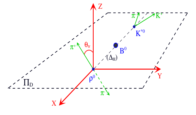
Figure 1: Transversity frame for $B\to\rho^{0}K^{*}$.

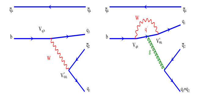
Figure 2: Tree diagram (left), and QCD-penguin diagram (right), for $B$ decays.

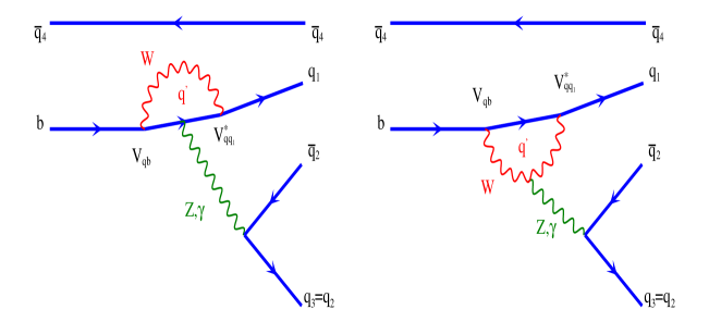
Figure 3: Electroweak-penguin diagram (left), and electroweak-penguin diagram with coupling between $Z,\gamma$ and $W$ (right), for $B$ decays.

Figure 4: Spectrum of ${\rho^{0}}-{\omega}$ mixing (in MeV/$c^{2}$), simulated by the interference of two Breit-Wigner curves.

Figure 5: Spectrum of $h_{--},h_{00},h_{++}$. Histograms on the left correspond to the channel $B^{0}\rightarrow\rho^{0}(\omega)K^{*0}$ where the parameters used are: ${q^{2}}/{{m^{2}}_{b}}=0.3$, $N_{c}^{eff}=2.84$, $\rho=0.229,\eta=0.325$ and form factors from the GH model. Histograms on the right correspond to the channel $B^{+}\rightarrow\rho^{0}(\omega)\rho^{+}$ for the same parameters with $N_{c}^{eff}=2.01$.

Figure 6: Spectrum of $\mathscr{R}\!e{(h_{ij})}\;{\rm and}\;\mathscr{I}\!m{(h_{ij})}$ where $i\neq j$. Histograms correspond to channel $B^{0}\rightarrow\rho^{0}(\omega)K^{*0}$ where the used parameters are: ${q^{2}}/{{m^{2}}_{b}}=0.3$, $N_{c}^{eff}=2.84$, $\rho=0.229,\eta=0.325$ and form factors from the GH model.

Figure 7: Spectrum of $\mathscr{R}\!e{(h_{ij})}\;{\rm and}\;\mathscr{I}\!m{(h_{ij})}$ where $i\neq j$. Histograms correspond to the channel $B^{+}\rightarrow\rho^{0}(\omega)\rho^{+}$ where the used parameters are: ${q^{2}}/{{m^{2}}_{b}}=0.3$, $N_{c}^{eff}=2.01$, $\rho=0.229,\eta=0.325$ and form factors from the GH model.

Figure 8: Spectrum of polar angle (upper figure) and azimuthal angle (lower one) in the helicity frame for the channel $B^{0}\rightarrow\rho^{0}(\omega)K^{*0}$. Parameters used are: ${q^{2}}/{{m^{2}}_{b}}=0.3$, $N_{c}^{eff}=2.84$, $\rho=0.229,\eta=0.325$ and form factors from the GH model.

Figure 9: Spectrum of polar angle (upper figure) and azimuthal angle (lower one) in the transversity frame for the channel $B^{0}\rightarrow\rho^{0}(\omega)K^{*0}$. Parameters are: ${q^{2}}/{{m^{2}}_{b}}=0.3$, $N_{c}^{eff}=2.84$, $\rho=0.229,\eta=0.325$ and form factors from the GH model.

Figure 10: $CP$-violating asymmetry parameter $a_{CP}(m)$, as a function of the ${\pi}^{+}{\pi}^{-}$ invariant mass in the vicinity of the $\omega$ mass region for the channel $B^{0}\rightarrow\rho^{0}(\omega)K^{*0}$. Parameters are: ${q^{2}}/{{m^{2}}_{b}}=0.3$, $N_{c}^{eff}=2.84$, $\rho=0.229,\eta=0.325$. Solid triangles up and circles correspond to the BSW and GH form factor models respectively.

Figure 11: $CP$-violating asymmetry parameter $a_{CP}(m)$, as a function of the ${\pi}^{+}{\pi}^{-}$ invariant mass in the vicinity of the $\omega$ mass region for the channel $B^{+}\rightarrow\rho^{0}(\omega)\rho^{+}$. Parameters are: ${q^{2}}/{{m^{2}}_{b}}=0.3$, $N_{c}^{eff}=2.01$, $\rho=0.229,\eta=0.325$. Solid triangles down and circles correspond to the BSW and GH form factor models respectively.

$C_{i}(\mu)$ for $\mu=5$ GeV
	$C_{1}$	$-0.3125$
	$C_{2}$	$+1.1502$
$C_{3}$	$+0.0174$	$C_{5}$	$+0.0104$
$C_{4}$	$-0.0373$	$C_{6}$	$-0.0459$
$C_{7}$	$-1.050\times 10^{-5}$	$C_{9}$	$-0.0101$
$C_{8}$	$+3.839\times 10^{-4}$	$C_{10}$	$+1.959\times 10^{-3}$

Table 1: Wilson coefficients to the next-leading order (see the reference in text).

$C_{i}^{\prime}$	$q^{2}/m_{b}^{2}=0.3$	$q^{2}/m_{b}^{2}=0.5$
$C_{1}^{\prime}$	$-0.3125$	$-0.3125$
$C_{2}^{\prime}$	$+1.1502$	$+1.1502$
$C_{3}^{\prime}$	$+2.433\times 10^{-2}+1.543\times 10^{-3}i$	$+2.120\times 10^{-2}+2.174\times 10^{-3}i$
$C_{4}^{\prime}$	$-5.808\times 10^{-2}-4.628\times 10^{-3}i$	$-4.869\times 10^{-2}-1.552\times 10^{-2}i$
$C_{5}^{\prime}$	$+1.733\times 10^{-2}+1.543\times 10^{-3}i$	$+1.420\times 10^{-2}+5.174\times 10^{-3}i$
$C_{6}^{\prime}$	$-6.668\times 10^{-2}-4.628\times 10^{-3}i$	$-5.729\times 10^{-2}-1.552\times 10^{-2}i$
$C_{7}^{\prime}$	$-1.435\times 10^{-4}-2.963\times 10^{-5}i$	$-8.340\times 10^{-5}-9.938\times 10^{-5}i$
$C_{8}^{\prime}$	$+3.839\times 10^{-4}$	$+3.839\times 10^{-4}$
$C_{9}^{\prime}$	$-1.023\times 10^{-2}-2.963\times 10^{-5}i$	$-1.017\times 10^{-2}-9.938\times 10^{-5}i$
$C_{10}^{\prime}$	$+1.959\times 10^{-3}$	$+1.959\times 10^{-3}$

Table 2: Effective Wilson coefficients related to the tree operators, electroweak and QCD penguin operators (see the reference in text).

	$\alpha$	$\beta$	$\gamma$
$(\rho_{min},\eta_{min})$	$104^{o}47$	$19^{o}32$	$56^{o}21$
$(\rho_{min},\eta_{max})$	$93^{o}13$	$24^{o}31$	$62^{o}56$
$(\rho_{max},\eta_{min})$	$112^{o}14$	$21^{o}20$	$46^{o}66$
$(\rho_{max},\eta_{max})$	$99^{o}66$	$26^{o}56$	$53^{o}78$

Table 3: Values of the CKM unitarity triangle for limiting values of the CKM matrix elements.

			$B\rightarrow\rho$
	$h_{V}$	$h_{A_{0}}$ = $h_{A_{3}}$	$h_{A_{1}}$	$h_{A_{2}}$	$m_{V}$ (${\rm GeV}^{2}$)	$m_{A_{i}}$ (${\rm GeV}^{2}$)
model $(1)$	0.329	0.281	0.283	0.283	5.32	5.32
model $(2)$	0.394	0.345	0.345	0.345	5.32	5.32
			$B\rightarrow\omega$
	$h_{V}$	$h_{A_{0}}$ = $h_{A_{3}}$	$h_{A_{1}}$	$h_{A_{2}}$	$m_{V}$ (${\rm GeV}^{2}$)	$m_{A_{i}}$ (${\rm GeV}^{2}$)
model $(1)$	0.328	0.280	0.281	0.281	5.32	5.32
model $(2)$	0.394	0.345	0.345	0.345	5.32	5.32
			$B\rightarrow K^{*}$
	$h_{V}$	$h_{A_{0}}$ = $h_{A_{3}}$	$h_{A_{1}}$	$h_{A_{2}}$	$m_{V}$ (${\rm GeV}^{2}$)	$m_{A_{i}}$ (${\rm GeV}^{2}$)
model $(1)$	0.369	0.321	0.328	0.331	5.43	5.43
model $(2)$	0.443	0.360	0.402	0.416	5.43	5.43

Table 4: Form factor values for $B\rightarrow\rho$, $B\rightarrow\omega$ and $B\rightarrow K^{*}$ at $q^{2}=0$ (see the reference in text).

channel	$\frac{q^{2}}{m_{b}^{2}}$	BSW	GH
	$0.3$	$2.1$	$1.0$
$\bar{B}^{0}\to\bar{K}^{*0}\rho^{0}(\omega)$
	$0.5$	$1.5$	$0.73$
	$0.3$	$6.6$	$3.9$
$B^{-}\to K^{*-}\rho^{0}(\omega)$
	$0.5$	$6.2$	$3.6$
	$0.3$	$24$	$13$
$B^{-}\to\rho^{-}\rho^{0}(\omega)$
	$0.5$	$24$	$14$

Table 5: $\bar{B}^{0},B^{-}$ branching ratios (in units of $10^{-6}$) using either the BSW or GH form factor models, for $q^{2}/m_{b}^{2}=0.3(0.5)$, with $N_{cmax}^{b\to s}=2.84(2.82)$, $N_{cmax}^{b\to d}=2.01(1.95)$, $\rho=0.229$ and $\eta=0.325$.

channel	$\frac{q^{2}}{m_{b}^{2}}$	BSW	GH
	$0.3$	$2.1$	$1.0$
$B^{0}\to K^{*0}\rho^{0}(\omega)$
	$0.5$	$1.7$	$0.88$
	$0.3$	$5.8$	$3.4$
$B^{+}\to K^{*+}\rho^{0}(\omega)$
	$0.5$	$3.8$	$2.3$
	$0.3$	$20$	$11$
$B^{+}\to\rho^{+}\rho^{0}(\omega)$
	$0.5$	$20$	$11$

Table 6: $B^{0},B^{+}$ branching ratios (in units of $10^{-6}$) using either the BSW or GH form factor models, for $q^{2}/m_{b}^{2}=0.3(0.5)$, with $N_{cmax}^{b\to s}=2.84(2.82)$, $N_{cmax}^{b\to d}=2.01(1.95)$, $\rho=0.229$ and $\eta=0.325$.

channel	$\frac{q^{2}}{m_{b}^{2}}$	BSW	GH
	$0.3$	$+0.36$	$-0.45$
$\bar{K}^{*0}(K^{*0})\rho^{0}(\omega)$
	$0.5$	$+4.70$	$+5.90$
	$0.3$	$-6.6$	$-6.37$
$K^{*-}(K^{*+})\rho^{0}(\omega)$
	$0.5$	$-23.0$	$-22.0$
	$0.3$	$-8.5$	$-9.6$
$\rho^{-}(\rho^{+})\rho^{0}(\omega)$
	$0.5$	$-8.7$	$-9.9$

Table 7: Global $CP$-violating asymmetries (in percents) using either the BSW or GH form factor models, for $q^{2}/m_{b}^{2}=0.3(0.5)$, with $N_{cmax}^{b\to s}=2.84(2.82)$, $N_{cmax}^{b\to d}=2.01(1.95)$, $\rho=0.229$ and $\eta=0.325$.

References

- [1] A.B. Carter and A.I. Sanda, Phys. Rev. Lett. 45 (1980) 952, Phys. Rev. D23 (1981) 1567; I.I. Bigi and A.I. Sanda, Nucl. Phys. B193 (1981) 85.
- [2] Proceedings of the Workshop on Violation, Adelaide 1998, edited by X.-H. Guo, M. Sevior and A.W. Thomas (World Scientific, Singapore).
- [3] A. Bozek (BELLE Collaboration), in Proceedings of the 4th International Conference on Physics and Violation, Ise-Shima, Japan, February 2001, hep-ex/0104041; K. Abe, et al. (BELLE Collaboration), in Proceedings of the XX International Symposium on Lepton and Photon Interactions at High Energies, July 2001, Roma, Italy, BELLE-CONF-0115 (2001); K. Abe, et al. (BELLE Collaboration), Phys. Rev. D65 (2002) 092005; R.S. Lu, et al. (BELLE Collaboration), Phys. Rev. Lett. 89 (2002) 191801.
- [4] T. Schietinger (BABAR Collaboration), Proceedings of Lake Louise Winter Institute on Fundamental Interactions, Alberta, Canada, February 2001, hep-ex/0105019; B. Aubert, et al. (BABAR Collaboration), hep-ex/0008058; B. Aubert, et al. (BABAR Collaboration), Phys. Rev. Lett. 87 (2001) 221802.
- [5] I. Dunietz et al, Phys. Rev. D43 (1991) 2193.
- [6] M.E. Rose, ”Elementary theory of angular momentum”, Dover.
- [7] A. Bohr, Nuclear Physics 10 (1959) 486.
- [8] H. Quinn, ”Hadronic effects in two-body B decays”. Lectures at SLAC Summer Institute (1999).
- [9] J. Schwinger, Phys. Rev. 12 (1964) 630; D. Farikov and B. Stech, Nucl. Phys. B133 (1978) 315; N. Cabibbo and L. Maiani, Phys. Lett. B73 (1978) 418; M.J. Dugan and B. Grinstein, Phys. Lett. B255 (1991) 583.
- [10] M. Bauer, B. Stech and M. Wirbel, Z. Phys. C34 (1987) 103; M. Wirbel, B. Stech and M. Bauer, Z. Phys. C29 (1985) 637.
- [11] M. Beneke, G. Buchalla, M. Neubert and C. T. Sachrajda, Nucl. Phys. B591 (2000) 313.
- [12] S. Gardner, H. B. O’Connell and A. W. Thomas, Phys. Rev. Lett. 80 (1998) 1834 [arXiv:hep-ph/9705453].
- [13] The Particle Data Group, D.E. Groom et al., Eur. Phys. J. C15 (2000) 1.
- [14] J.J. Sakurai, Currents and Mesons, University of Chicago Press (1969).
- [15] H.B. O’Connell, B.C. Pearce, A.W. Thomas and A.G. Williams, Prog. Part. Nucl. Phys. 39 (1997) 201; H.B. O’Connell, A.G. Williams, M. Bracco and G. Krein, Phys. Lett. B370 (1996) 12; H.B. O’Connell, Aust. J. Phys. 50 (1997) 255.
- [16] X.-H. Guo and A.W. Thomas, Phys. Rev. D58 (1998) 096013, Phys. Rev. D61 (2000) 116009.
- [17] H.B. O’Connell, A.W. Thomas and A.G. Williams, Nucl. Phys. A623 (1997) 559; K. Maltman, H.B. O’Connell and A.G. Williams, Phys. Lett. B376 (1996) 19.
- [18] S. Gardner and H.B. O’Connell, Phys. Rev. D57 (1998) 2716.
- [19] L. Wolfenstein, Phys. Rev. Lett. 51 (1983) 1945, Phys. Rev. Lett. 13 (1964) 562.
- [20] A.J. Buras, Lect. Notes Phys. 558 (2000) 65, also in ‘Recent Developments in Quantum Field Theory’, Springer Verlag, edited by P. Breitenlohner, D. Maison and J. Wess (Springer-Verleg, Berlin, in press), hep-ph/9901409.
- [21] V.A. Novikov, M.A. Shifman, A.I. Vainshtein and V.I. Zakharov, Nucl. Phys. B249 (1985) 445, Yad. Fiz. 41 (1985) 1063.
- [22] M.A. Shifman, A.I. Vainshtein and V.I. Zakharov, Nucl. Phys. B147 (1979) 385, Nucl. Phys. B147 (1979) 448.
- [23] A.J. Buras, Published in ‘Probing the Standard Model of Particle Interactions’, eds. 1998, Elsevier Science B.V., hep-ph/9806471.
- [24] N.G. Deshpande and X.-G. He, Phys. Rev. Lett. 74 (1995) 26.
- [25] R. Fleischer, Int. J. Mod. Phys. A12 (1997) 2459, Z. Phys. C62 (1994) 81, Z. Phys. C58 (1993) 483.
- [26] G. Kramer, W. Palmer and H. Simma, Nucl. Phys. B428 (1994) 77.
- [27] R. Enomoto and M. Tanabashi, Phys. Lett. B386 (1996) 413.
- [28] G. Buchalla, A.J. Buras and M.E. Lautenbacher, Rev. Mod. Phys. 68, (1996) 1125.
- [29] X.-H. Guo and T. Huang, Phys. Rev. D43 (1991) 2931.
- [30] Y.-H. Chen, H.-Y. Cheng, B. Tseng and K.-C. Yang, Phys. Rev. D60 (1999) 094014.
- [31] By ALEPH, CDF, DELPHI, L3, OPAL and SLD Collaborations (D. Abbaneo et al.), hep-ex/0112028.
- [32] H.-Y. Cheng and A. Soni, Phys. Rev. D64 (2001) 114013.
- [33] D. Melikhov and B. Stech, Phys. Rev. D62 (2000) 014006.
- [34] O. Leitner, X.-H. Guo and A.W. Thomas, Phys. Rev. D66 (2002) 096008; X.-H. Guo, O. Leitner and A.W. Thomas, Phys. Rev. D63 (2001) 056012.
- [35] P. Langacker, Phys. Rev. D20 (1979) 2983.
- [36] T. Affolder et al., Phys. Rev. Let. 85, 4668 (November 2000) and references therein.
- [37] J.D. Jackson, Il Nuovo Cimento, Vol.XXXIV, (1964) 1644.
- [38] De Wit and J. Smith, Field Theory in Particle Physics, Nort-Holland (1986).