Extraction of the $x$-dependence of the non-perturbative QCD $b$-quark fragmentation distribution component.
E. Ben-Haim^1,2, Ph. Bambade¹, P. Roudeau¹, A. Savoy-Navarro^2,3
and A. Stocchi¹

(1) U. de Paris-Sud, Lab. de l’Accélérateur Linéaire (L.A.L.), Orsay and IN2P3-CNRS

(2) LPNHE, Universités de Paris 6-7 and IN2P3-CNRS

(3) Also Visitor at Fermilab in the CDF experiment

Using recent measurements of the $b$-quark fragmentation distribution obtained in $e^{+}e^{-}\rightarrow b\overline{b}$ events registered at the ${\rm Z}$ pole, the non-perturbative QCD component of the distribution has been extracted independently of any hadronic physics modelling. This distribution depends only on the way the perturbative QCD component has been defined. When the perturbative QCD component is taken from a parton shower Monte-Carlo, the non-perturbative QCD component is rather similar with those obtained from the Lund or Bowler models. When the perturbative QCD component is the result of an analytic NLL computation, the non-perturbative QCD component has to be extended in a non-physical region and thus cannot be described by any hadronic modelling. In the two examples used to characterize these two situations, which are studied at present, it happens that the extracted non-perturbative QCD distribution has the same shape, being simply translated to higher-$x$ values in the second approach, illustrating the ability of the analytic perturbative QCD approach to account for softer gluon radiation than with a parton shower generator.

1 Introduction

Improved determinations of the $b$-quark fragmentation distribution have been obtained by ALPEH [1], DELPHI [2], OPAL [3] and SLD [4] collaborations which measured the fraction of the beam energy taken by a weakly decaying $b$-hadron in $e^{+}e^{-}\rightarrow b\overline{b}$ events registered at, or near, the ${\rm Z}$ pole.

This distribution is generally viewed as resulting from three components: the primary interaction ($e^{+}e^{-}$ annihilation into a $b\overline{b}$ pair in the present study), a perturbative QCD description of gluon emission by the quarks and a non-perturbative QCD component which incorporates all mechanisms at work to bridge the gap between the previous phase and the production of weakly decaying $b$-mesons. The perturbative QCD component can be obtained using analytic expressions or Monte Carlo generators. The non-perturbative QCD component is usually parametrized phenomenologically via a model.

To compare with experimental results, one must fold both components to evaluate the expected $x$-dependence:

$${\cal D}_{predicted}(x)=\int_{0}^{1}{{\cal D}_{pert.}(z)\times{\cal D}_{non-pert.}^{model}(\frac{x}{z})~{}\frac{dz}{z}}$$ (1)

The final and the perturbative components are defined over the $[0,1]$ interval. As explained, in the following, the non-perturbative distribution must be evaluated for $x>1$, if the perturbative component is non-physical. The parameters of the model are then fitted by comparing the measured and predicted $x$-dependence of the $b$-quark fragmentation distribution. Such comparisons have already been made by the different experiments using, for the perturbative component, expectations from generators such as the JETSET or HERWIG parton shower Monte-Carlo. It has been shown, with present measurement accuracy, that most of existing models, for the non-perturbative part, are unable to give a reasonable fit to the data [1, 2, 3, 4]. Best results have been obtained with the Lund and Bowler models [11, 12].

In the following, a method is presented to extract the non-perturbative QCD component of the fragmentation function directly from data, independently of any hadronic model assumption. This distribution can then be compared with models to learn about the non-perturbative QCD transformation of $b$-quarks into $b$-hadrons. It can then be used in another environment than $e^{+}e^{-}$ annihilation, as long as the same parameters and methods are taken for the evaluation of the perturbative QCD component. Consistency checks, on the matching between the measured and predicted $b$-fragmentation distribution, can be defined which provide information on the determination of the perturbative QCD component itself.

In Section 2, the method used to extract the non-perturbative QCD component is presented.

In Section 3, the extraction is performed for two determinations of the perturbative QCD component using:

• the JETSET 7.3 generator [5], tuned on DELPHI data [6], running in the parton shower mode,

• an analytic computation based on QCD at NLL order [7].

In Section 4 these results are discussed and insights obtained with the present analysis are explained. A parametrization for the non-perturbative QCD component is proposed.

2 Extracting the $x$-dependence of the non-perturbative
QCD component

The method is based on the use of the Mellin transformation which is appropriate when dealing with integral equations as given in (1). The Mellin transformation of the expression for ${\cal D}(x)$ is:

$$\tilde{{\cal D}}(N)=\int_{0}^{\infty}{dx~{}x^{N-1}~{}{\cal D}(x)}$$ (2)

where $N$ is a complex variable. For integer values of $N\geq 2$, the values of $\tilde{{\cal D}}(N)$ correspond to the moments of the initial $x$ distribution . For physical processes, $x$ is restricted to be within the $[0,1]$ interval. The interest in using Mellin transformed expressions is that Equation (1) becomes a simple product:

$$\tilde{{\cal D}}(N)=\tilde{{\cal D}}_{pert.}(N)\times\tilde{{\cal D}}_{non-pert.}(N)$$ (3)

Having computed, in the $N$-space, distributions of the measured and perturbative QCD components, the non-perturbative distribution, $\tilde{{\cal D}}_{non-pert.}(N)$ is obtained from Equation (3). Applying the inverse Mellin transformation on this distribution one gets ${\cal D}_{non-pert.}(x)$ without any need for a model input:

$${\cal D}_{non-pert.}(x)=\frac{1}{2\pi i}\oint{dN~{}\frac{\tilde{{\cal D}}_{meas.}(N)}{\tilde{{\cal D}}_{pert.}(N)}~{}x^{-N}}$$ (4)

in which the integral runs over a contour in the complex $N$-plane. The integration contour is taken as two symmetric straight half-lines, one in the upper half and the other in the lower half of the complex plane. The angle of the lines, relative to the real axis, is larger or smaller than 90 degrees for $x$ values smaller or larger than unity, respectively. These lines are taken to originate from $N=(1.01,0)$. The contour is supposed to be closed by an arc situated at infinity in the negative and positive directions of the real axis, for the two cases respectively .

,

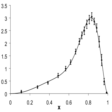
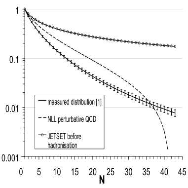
Figure 1: Left: Comparison between the measured (points with error bars) $b$-fragmentation distribution and the fitted parametrization using Equation (5). Right: Moments of the measured (full line) $x$ distribution, of the perturbative QCD component [7](dashed line) and of the generated distribution obtained in JETSET before hadronization (full line with circles). Data from [1] have been used.

In practice, the Mellin transformed distribution of present measurements, $\tilde{{\cal D}}_{meas.}(N)$, has been obtained after having adjusted an analytic expression to the measured distribution in $x$, and by applying the Mellin transformation on this fitted function. The following expression, which depends on five parameters and gives a good description of the measurements (see Figure 1-left), has been used.

$$D(x)=p_{0}\times\left[p_{1}x^{p_{2}}(1-x)^{p3}+(1-p_{1})x^{p_{4}}(1-x)^{p5}\right]$$ (5)

where $p_{0}$ is a normalisation coefficient. Values of the parameters have been obtained by comparing, in each bin, the measured bin content with the integral of $D(x)$ over the bin.

Measurements of the $b$-fragmentation distribution, in [1], have been published in a binned form, after unfolding of the experimental energy resolution. Values in the bins are correlated and, as the bin width is smaller than the resolution, the error matrix is singular. Only positive eigenvalues of this matrix have been used in the present analysis, when fitting parameters.

The distribution of moments obtained with data from [1], and computed using the fitted distribution corresponding to Equation (5), is given in Figure 1-Right. The corresponding analytic expression is:

$$\tilde{{\cal D}}(N)=p_{0}\left[p_{1}\frac{\Gamma(p_{2}+N)}{\Gamma(p_{2}+p_{3}+N+1)}+(1-p_{1})\frac{\Gamma(p_{4}+N)}{\Gamma(p_{4}+p_{5}+N+1)}\right]$$ (6)

Quoted uncertainties, in Figure 1-Right, correspond to actual measurements and are highly correlated. They have been obtained by propagating uncertainties corresponding to the covariance matrix of the $p_{1,.,5}$ fitted parameters. When computing the moments, very similar results are obtained, for $N<10$, using directly the measured $x$-binned distribution. For higher $N$ values effects induced by the variation of the distribution within a bin, as expressed by Equation (5), have to be included.

The Mellin transformed distribution of the JETSET perturbative QCD component has been obtained in a similar way, whereas the NLL QCD perturbative component is computed directly as a function of $N$ in [7]. At large values of $N$, this last distribution is equal to zero for $N=N_{0}\simeq 41.7$ and has a Landau pole situated at $N_{L}\simeq 44.$

3 $x$-dependence measurement of the non-perturbative QCD component

The $x$ distribution of the non-perturbative QCD component extracted in this way depends on the measurements and also on the procedures adopted to compute the perturbative QCD component. In the following two approaches have been considered. The first one is generally adopted by experimentalists whereas the second is more frequent for theorists.

3.1 The perturbative QCD component is provided by a generator

The JETSET 7.3 Monte Carlo generator, with values of the parameters tuned on DELPHI data registered at the ${\rm Z}$ pole has been used. Events have been produced using the parton shower option of the generator and the $b$-quark energy is extracted, after radiation of gluons, just before calling the routines to create a $b$-hadron that takes a fraction $z$ of the available string energy. This distribution is displayed in Figure 2. It has to be complemented by a $\delta$-function at $x=1$ which contains $\sim 4\%$ of all events. In this peak, $b$-hadrons carry all the energy of the $b$-quark as no gluon has been radiated.

Applying the method explained in Section 2, the corresponding non-perturbative QCD component has been extracted, and is displayed also in Figure 2. Above $x=1$, it is compatible with zero, as expected. The quoted error bar, for a given value of $x$, has been obtained by evaluating the values of ${\cal D}_{non-pert.}(x)$ for different shapes of the $b$-quark fragmentation distribution which are obtained by varying parameters $p_{1,.,5}$ according to their measured error matrix.

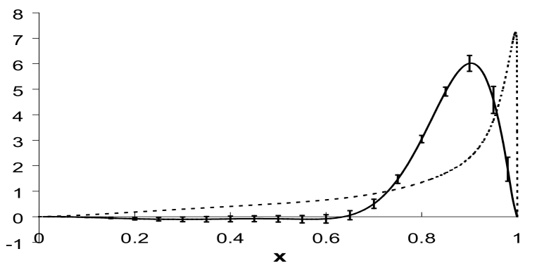
Figure 2: $x$-dependence of the perturbative (dotted line) and non-perturbative (full line) QCD components of the measured [1] $b$-fragmentation distribution. These curves are obtained by interpolating corresponding values determined at a large number of points in the x-variable. Quoted error bars correspond to measurement uncertainties and are correlated for different $x$-values. The perturbative QCD component is extracted from the JETSET 7.3 Monte Carlo generator. The dotted curve has to be complemented by a $\delta$-function containing 4$\%$ of the events, located at $x=1$.

3.2 The perturbative QCD component is obtained by an analytic computation based on QCD

The perturbative QCD fragmentation function is evaluated according to the approach presented in [7]. This next to leading log (NLL) accuracy calculation for the inclusive $b$-quark production cross section in $e^{+}e^{-}$ annihilation, generalises previous calculations by resumming the contribution from soft gluon radiation (which plays an important role at large $x$) to all perturbative orders and to NLL accuracy. These computations are done directly in the $N$-space. Soft gluon radiation contributes to the logarithm of the fragmentation function large logarithmic terms of the type $(\log{N})^{p}$, with $p\leq n+1$. These terms appear at all perturbative orders $n$ in $\alpha_{s}$. In the calculation at NLL accuracy [7], the two largest terms, corresponding to $p=n+1~{}{\rm and}~{}n$, have been resummed at all perturbative orders. The calculation is expected to be reliable when $N$ is not too large (typically less than 20). To obtain distributions for the variable $x$ from results in moment space, one should apply the inverse Mellin transformation, that consists in integrating over a contour in $N$ (Section 2). When $x$ gets closer to 1, large values of $N$ contribute and thus the perturbative fragmentation distribution is not reliable in these regions. This behaviour affects also values of the distribution at lower $x$ as moments of this distribution are fixed. In addition to the break-down of the theory for large values of $N$, uncertainties attached to the determination of the theoretical perturbative QCD component are related to the definition of the scales entering into the computation. This component also depends on two parameters: the $b$-quark pole mass ($m_{b}$) and $\Lambda^{(5)}_{QCD}$, that have been taken as $m_{b}^{pole}=(4.75\pm 0.25)~{}\rm{GeV}/c^{2}$ and $\Lambda^{(5)}_{QCD}=(0.226\pm 0.025)~{}\rm{GeV}$. Scale and parameter depending variations of the moments of the perturbative QCD component are given in Figure 3. These variations are fully correlated versus $N$.

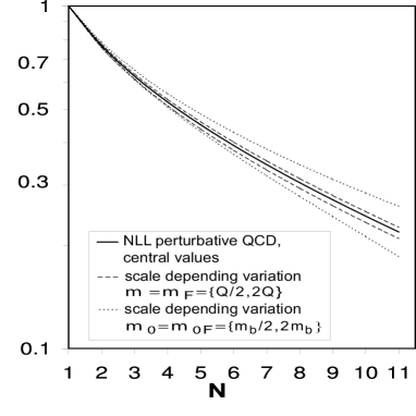
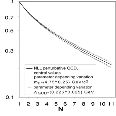
Figure 3: Variations of the calculated perturbative QCD component [7], depending on the renormalization scales ($\mu$, $\mu_{0}$), the factorisation scales ($\mu_{F}$, $\mu_{0F}$), the $b$-quark mass ($m_{b}$) and $\Lambda^{(5)}_{QCD}$. The full lines are corresponding to the central values ($\mu=\mu_{F}=Q=91.2~{}\rm{GeV}$, $\mu_{0}=\mu_{0F}=m_{b}$, $m_{b}=4.75~{}\rm{GeV}/c^{2}$ and $\Lambda^{(5)}_{QCD}=0.226~{}\rm{GeV}$).

The extracted non-perturbative component is given in Figure 4. Its shape depends on the same quantities as those used to evaluate the perturbative distribution, and thus similar variations appear, as drawn also in the Figure.

It has to be noted that the data description in terms of a product of two QCD components, perturbative and non-perturbative, is not directly affected by uncertainties attached to the determination of the perturbative component. This is because the non-perturbative component, as determined in the present approach, compensates for a given choice of method or of parameter values.

To obtain the complete expected $x$-distribution of $b$-hadrons from the theoretical calculation, one has to be able to evaluate the integral given in Equation (1). When $x$ becomes close to 1 there are numerical problems, and consequently, the high-$x$ ($x>0.96$) behaviour of the perturbative QCD component has been studied. As mentioned before, this region corresponds to high-N values where the perturbative approach fails. As a result, the high-$x$ behaviour of the distribution is non-physical; it oscillates. To have a numerical control of the distribution in this region, it has been decided to take into account $x$ values which are below a given maximum value, $x_{max}$, above which the distribution is assumed to be equal to zero. Moments of this truncated distribution show a small discrepancy when compared with moments of the full distribution. This difference has an almost linear dependence with $N$. To correct for this effect, $x_{max}$ is chosen such that the difference between moments is a constant value (the slope in $N$ being close to zero at this point). This difference can then be corrected by adding simply a $\delta$-function at $x=1$, so that the total distribution is normalized to 1. A typical value for $x_{max}$ is 0.997 and the $\delta$ component corresponds to 5$\%$ of the distribution. We stress that the truncation at $x_{max}$ and the added $\delta$-function do not contribute in the determination of the non-perturbative component using Equation (4). But this procedure is necessary for checking that the extracted non-perturbative component in the $x$-space, when convoluted with the perturbative distribution, effectively reproduces the measurements and also for testing hadronic models given in the $x$-space.

Conversely to the perturbative QCD component which was, by definition in [7], defined within the $[0,1]$ interval, the non-perturbative component has to be extended in the region $x>1$. This “non-physical” behaviour comes from the zero of $\tilde{{\cal D}}_{pert.}(N)$ for $N=N_{0}$ which gives a pole in the expression to be integrated in Equation (4). Using properties of integrals in the complex plane, it can be shown that, for $x>1$, the non-perturbative QCD distribution can be well approximated by $x^{-N_{0}}$.

Errors bars, given in Figure 4, have been obtained using the same procedure as explained in Section 3.2.

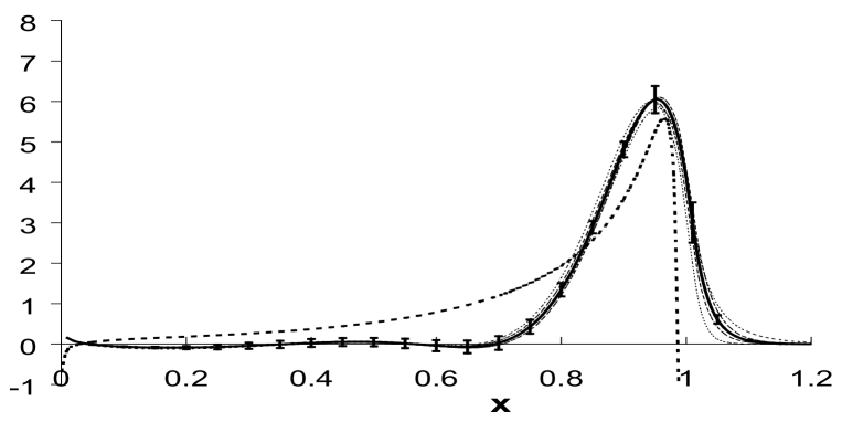
Figure 4: $x$-dependence of the perturbative (dotted line) and non-perturbative (full line) QCD components of the measured $b$-fragmentation distribution. These curves are obtained by interpolating corresponding values determined at a large number of points in the x-variable. The perturbative QCD component is given by the analytic computation of [7]. The thin lines on both sides of the non-perturbative distribution are corresponding to $\mu_{0}=\mu_{0F}=\{m_{b}/2,2m_{b}\}$ (dotted lines) and $\Lambda^{(5)}_{QCD}=(0.226\pm 0.025)~{}\rm{GeV}$ (dashed lines). Variations induced by the other parameters, $\mu=\mu_{F}=\{Q/2,2Q\}$ and $m_{b}=(4.75\pm 0.25)~{}\rm{GeV}/c^{2}$ are smaller. In addition, quoted error bars correspond to measurement uncertainties and are correlated for different $x$-values. The perturbative QCD dotted curve has to be complemented by a $\delta$-function containing 5$\%$ of the events, located at $x=1$.

4 Results interpretation

The $x$-dependence of the non-perturbative QCD component, obtained in this way, does not depend on any non-perturbative QCD model assumption but its shape is tightly related to the procedures used to evaluate the perturbative component, and thus, the two distributions have to be used jointly.

4.1 Comparison with models

Non-perturbative components of the $b$-quark fragmentation distribution, taken from models, have been folded with a perturbative QCD component obtained from a Monte Carlo generator and compared with measurements by the different collaborations [1, 2, 3, 4]. Apart for the Lund and Bowler models, none of the other models provided a good fit to the data. In Figure 5 the directly extracted non-perturbative components are compared with distributions taken from models [8, 9, 10, 11, 12] whose parameters have been fitted on data from [1]. Results have been obtained by comparing, in each bin, the measured bin content with the integral, over the bin, of the folded expression for ${\cal D}_{predicted}(x)$. They are summarized in Table 1. It must be noted that parameters given in this Table, when the perturbative QCD component is taken from JETSET, may differ from those quoted in original publications as an analytic computation is done in the present study, using Equation (1), whereas a string model is used in the former; other sources of difference can originate from the exact values of the parameters used to run JETSET and from the definition of $x$ which varies between 0 and 1 in our case. Numerically, if one compares present results with those obtained by OPAL [3], in their own analysis, for the values of the parameters of the Lund and Bowler models , differences are well within uncertainties.

Model	JETSET		NLL Pert. QCD
	param.	$\chi^{2}/NDF$	param.	$\chi^{2}/NDF$
Kartvelishvili [8]	$\epsilon_{b}=13.2^{+0.8}_{-0.7}$	$27/4$	$\epsilon_{b}=14.0\pm 0.7$	$22/4$
$x^{\epsilon_{b}}(1-x)$
Peterson [9]	$\epsilon_{b}=(5.6^{+0.7}_{-0.6})\times 10^{-3}$	$62/4$	$\epsilon_{b}=(3.1\pm 0.5)\times 10^{-3}$	$29/4$
$\frac{1}{x}\left(1-\frac{1}{x}-\frac{\epsilon_{b}}{1-x}\right)^{-2}$
C.S [10]	$\epsilon_{b}=(5.4^{+0.9}_{-0.8})\times 10^{-3}$	$144/4$	$\epsilon_{b}=(4.4^{+1.5}_{-1.1})\times 10^{-4}$	$18/4$
$\left(\frac{1-x}{x}+\frac{\epsilon_{b}(2-x)}{1-x}\right)\left(1+x^{2}\right)\left(1-\frac{1}{x}-\frac{\epsilon_{b}}{1-x}\right)^{-2}$
Lund [11]	$a=1.55\pm 0.15$	$2.6/3$	$a=0.04\pm 0.09$	$0.5/3$
$\frac{1}{x}(1-x)^{a}\exp{\left(-\frac{bm_{b\bot}^{2}}{x}\right)}$	$bm_{b\bot}^{2}=14.7^{+1.4}_{-1.2}$		$bm_{b\bot}^{2}=8.8^{+0.9}_{-0.8}$
Bowler [12]	$a=0.77^{+0.15}_{-0.12}$	$2.5/3$	$a=0.00\pm 0.03$	$4.4/3$
$\frac{1}{x^{1+bm_{b\bot}^{2}}}(1-x)^{a}\exp{\left(-\frac{bm_{b\bot}^{2}}{x}\right)}$	$bm_{b\bot}^{2}=63.7^{+6.8}_{-6.0}$		$bm_{b\bot}^{2}=53.\pm 6.$

Table 1: Values of the parameters and of the $\chi^{2}/NDF$ obtained when fitting results from Equation (1), obtained for different models of the non-perturbative QCD component, to the measured $b$-fragmentation distribution. The two situations corresponding, respectively, to the perturbative QCD component taken from JETSET or from [7] have been distinguished. The Lund and Bowler models have been simplified by assuming that the transverse mass of the $b$-quark, $m_{b\bot}$, is a constant.

When the perturbative QCD component is taken from the analytic NLL calculation the Lund and Bowler models give also the best description of the measurements. Values for the parameter $a$ in these models are even compatible with zero corresponding to a behaviour in $1/z^{\alpha}~{}\exp{(-A/z)}$, to accomodate the non-zero value of the non-perturbative QCD component at $x=1$.

But, as these models have no contribution above $x=1$, their folding with the perturbative QCD component cannot compensate for the non-physical behaviour of the latter. The folded distribution is oscillating at large $x$-values (see Figure 6-Left). In particular, the predicted value in the last measured $x$-bin, which is found to be in reasonable agreement with the measurements after the fitting procedure when using the Lund and Bowler models, results from a large cancellation between a negative and a positive contribution within that bin. This is more clearly seen when considering the moments of the overall distribution, which are given by Equation (3). For moments of order $N$, the weight $x^{N-1}$ introduces a variation within the $x$-bin size, which was not accounted for in the previous fit in $x$, and effects are amplified mainly at large $N$ values which correspond to the high $x$ region. This is illustrated in Figure 6-Right.

From this study, it results that all models have to be discarded when folded with the NLL perturbative QCD fragmentation distribution. The goodness of the fit in $x$, as measured by the corresponding $\chi^{2}$ value, does not reflect all the information because it was not required that the folded distribution remains physical (positive) over the $[0,1]$ interval. This folding procedure has thus to be considered only as an exercise and the non-perturbative QCD distribution has to be extracted from data.

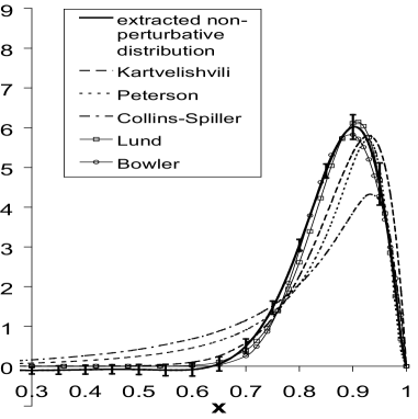
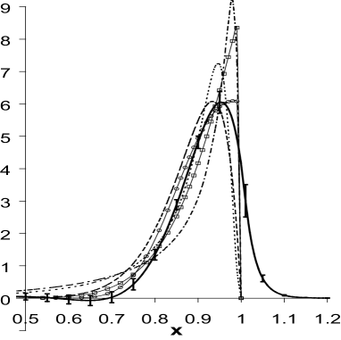
Figure 5: Comparison between the directly extracted non-perturbative component (thick full line) and the model fits on data taken from [1]. Left: the perturbative QCD component is taken from JETSET. Right: the theoretical perturbative QCD component[7] is used.

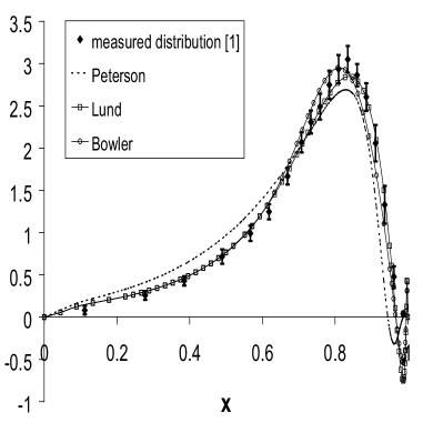
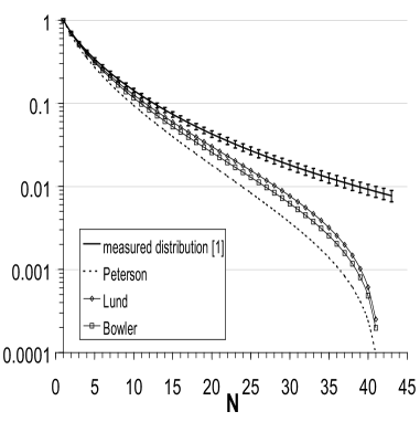
Figure 6: Comparison between the measured and fitted $x$-distributions using different models. Left: the measured binned-distribution in $x$ is compared with fitted results. Right: moments of the corresponding distributions are compared.

4.2 Proposal for a new parametrization

As explained in Section 2, the non-perturbative QCD component of the $b$-fragmentation distribution, has been extracted independently of any hadronic model assumption but it depends on the modelling of the perturbative QCD component.

When a Monte-Carlo generator is used to obtain the perturbative component, it can be verified if the non-perturbative component has a physical behaviour for all $x$-values. In Figure 2, below $x=0.6$, $(4\pm 3)\%$ of the integrated distribution is negative. A larger deviation would have indicated some inconsistancy between experimental measurements and gluon radiation, as implemented in the generator.

Such a test cannot be made, a priori, when the perturbative QCD component is taken from an analytic computation as this distribution is already unphysical in some regions. The non-perturbative extracted distribution, as given in Figure 4, is precisely expected to compensate for these effects. It can be noted that, also in this case, the distribution is compatible with zero below $x=0.6$. This shows that the perturbative QCD evaluation of hard gluon radiation is in agreement with the measurements. The small spike, close to $x=0$, related to the multiplicity problem [13] in the perturbative evaluation, has no numerical effect in practice.

To provide an analytic expression, which agrees better with the extracted point-to-point non-perturbative QCD distribution, the following function has been used:

$${\cal D}_{non-pert.}(x) = N({\bf p})\exp{-\frac{(x-x_{0})^{2}}{2\sigma_{-}^{2}}}~{}{\rm for}~{}x<x_{0};$$ (7)

$$= N({\bf p})\exp{-\frac{(x-x_{0})^{2}}{2\sigma_{+}^{2}}}~{}{\rm for}~{}x_{0}<x<1;$$

$$= N({\bf p})x^{-N_{0}}~{}{\rm for}~{}x>1;~{}{\bf p}=(x_{0},\sigma_{-},\sigma_{+})$$

It corresponds, for $0<x<1$, to Gaussian distributions with different standard deviations when $x$ is situated on either sides of $x_{0}$. As explained in Section 2, the behaviour of the non-perturbative distribution for $x>1$ is related to the presence of a zero in ${\cal D}_{pert.}(N)$ located at $N=N_{0}$. When the perturbative distribution is taken from a Monte-Carlo, there is not such a zero and it has been considered that ${\cal D}_{non-pert.}(x)=0$ when $x>1$. When the perturbative distribution is taken from theory, the value of $N_{0}$ has been fixed to 41.7. The value for $N_{0}$ depends a lot on the central values for the parameters and the scales, adopted in the perturbative QCD evaluation :

$$N_{0}=41.7^{-5.8}_{+4.5}(\Lambda^{(5)}_{QCD})\pm 2.5(m_{b})^{+34.6}_{-21.7}(\mu_{0}=\mu_{0F})$$ (8)

$N({\bf p})$ is a normalisation factor such that the integral of the expression, given in Equation (7), between $0$ and $\infty$ is equal to unity.

The parameter values, obtained when the perturbative QCD component is taken either from JETSET or from theory, are given in Table 2. It can be noted that the shape of the non-perturbative QCD distribution is similar in the two cases, the maximum being displaced to an higher value in the latter.

	$x_{0}$	$\sigma_{-}$	$\sigma_{+}$	$\chi^{2}/NDF$
JETSET	$0.911\pm 0.006$	$0.088\pm 0.006$	$0.045\pm 0.005$	$3.0/2$
NLL pert. QCD	$0.955\pm 0.011$	$0.087\pm 0.006$	$0.06^{+0.04}_{-0.02}$	$0.7/2$

Table 2: Values for the fitted parameters of the non-perturbative QCD component corresponding to JETSET and NLL perturbative QCD using data from [1].

Comparison, in $x$- and in moment-space, between the measured and fitted distributions are given in Figure 7. For moments higher than 40, the fitted moments strongly deviate from the measurements as one is approaching the Landau pole and the formalism of [7] is no longer valid.

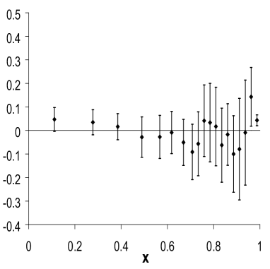
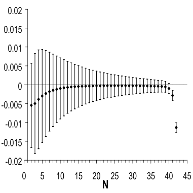
Figure 7: Comparison between the fitted and measured $b$-quark fragmentation distributions. Left: Differences between the fitted and the measured distributions in each $x$-bin are shown and the total error bars, relative to the measurements, are displayed. The fitted results correspond to the averaged values obtained from Equation (1) over the bin. Right: Differences between the fitted and measured moments of the $b$-fragmentation distribution. Fitted moments result from the product given in Equation (3) in which $\tilde{{\cal D}}_{non-pert.}(N)$ are the moments of the fitted non-perturbative QCD distribution corresponding to Equation (7) and $\tilde{{\cal D}}_{pert.}(N)$ corresponds to the analytic computation [7].

5 Conclusions

The measured $b$-quark fragmentation distribution has been analysed in terms of its perturbative and non-perturbative QCD components.

The $x$-dependence of the fragmentation distribution has been extracted in a way which is independent of any model for non-perturbative hadronic physics. It depends closely on the way the perturbative QCD component has been evaluated. The obtained distribution differs markedly from those expected from various models.

Below $x=0.6$, this distribution is compatible with zero indicating that most of gluon radiation is well accounted by the perturbative QCD component evaluated using the LUND parton shower Monte-Carlo or computed analytically.

As the non-perturbative QCD distribution is evaluated for any given value of the $x$-variable it can be verified if it remains physical over the interval $[0,1]$ when used with a Monte-carlo generator which provides the perturbative component. The evidence for unphysical regions would indicate that the simulation or the measurements are incorrect. There is not such an evidence in the present analysis.

Above $x=0.6$, the obtained distribution is similar in shape with those expected from the Lund symmetric [11] or Bowler [12] models, when the perturbative QCD component is taken from JETSET. This is no longer true, also for these two models, when the perturbative QCD component is taken from the analytic result of [7]. It has been found that, because of the analytic behaviour of the perturbative QCD component, the non-perturbative QCD distribution must be extended above $x=1$. The $x$-behaviour of the non-perturbative component, for $x>1$, is determined by the possible existence of a zero in $\tilde{{\cal D}}_{pert.}(N)$, for $N>0$. When the perturbative component has non-physical aspects, it is thus not justified to fold it with any given physical model. An approach has been proposed to solve this problem and a parametrization of the obtained distribution has been provided.

The non-perturbative component, extracted in this way, is expected to be valid in a different environment than $e^{+}e^{-}$ annihilation, as long as the perturbative QCD part is evaluated within the same framework (analytic QCD computation or a given Monte Carlo generator), and using the same values for the parameters entering into this evaluation as $m_{b}^{pole}$, $\Lambda^{(5)}_{QCD}$ or generator tuned quantities. It is planned to do a similar analysis using the improved analytic computation of the perturbative QCD $b$-fragmentation distribution given in [14].

6 Acknowledgements

We thank M. Cacciari, S. Catani and M. Fontannaz for their help to understand physical and technical aspects of the theory of $b$-quark fragmentation. We thank also our colleagues from DELPHI, from the Institute for Experimental Nuclear Physics, Karlsruhe University, for fruitful discussions.

The work of E. Ben-Haim is supported by EEC RTN contract HPRN-CT-00292-2002.

References

- [1] A. Heister et al., ALEPH Collaboration, Phys. Lett. B512 (2001) 30.
- [2] G. Barker et al., DELPHI Collaboration, DELPHI 2002-069 CONF 603.
- [3] G. Abbiendi et al., OPAL Collaboration, hep-ex/0210031, submitted to Eur. Phys. J. C.
- [4] K. Abe et al., SLD Collaboration, Phys. Rev. D65 (2002) 092006, Erratum-ibid. D66 (2002) 079905.
- [5] T.Sjöstrand, Comp. Phys. Comm. 82 (1994) 74.
- [6] DELPHI Collaboration P. Abreu et al., Zeit. Phys. C73 (1996) 11.
- [7] M. Cacciari and S. Catani, Nucl. Phys. B617 (2001) 253, hep-ph/0107138.
- [8] V.G. Kartvelishvili, A.K. Likehoded, V.A. Petrov, Phys. Lett. B78 (1978) 615.
- [9] C. Peterson, D. Schlatter, I. Schmitt, P.M. Zerwas, Phys. Rev. D27 (1983) 105.
- [10] P. Collins, T. Spiller, J. Phys. G11 (1985) 1289.z
- [11] B. Andersson, G. Gustafson, B. Soderberg, Z. Phys. C 20 (1983) 317.
- [12] M.G. Bowler, Z. Phys. C 11 (1981) 169.
- [13] A. Bassetto, M. Ciafaloni and G. Marchesini, Phys. Rep. 100 (1983) 201.
- [14] M. Cacciari and E. Gardi, hep-ph/0301047.