Yukawa Coupling Unification
in Supersymmetric Models

Abstract:

We present an updated assessment of the viability of $t-b-\tau$ Yukawa coupling unification in supersymmetric models. For the superpotential Higgs mass parameter $\mu>0$, we find unification to less than 1% is possible, but only for GUT scale scalar mass parameter $m_{16}\sim 8-20$ TeV, and small values of gaugino mass $m_{1/2}\stackrel{{\scriptstyle\scriptscriptstyle<}}{{\scriptscriptstyle\sim}}400$ GeV. Such models require that a GUT scale mass splitting exists amongst Higgs scalars with $m_{H_{u}}^{2}<m_{H_{d}}^{2}$. Viable solutions lead to a radiatively generated inverted scalar mass hierarchy, with third generation and Higgs scalars being lighter than other sfermions. These models have very heavy sfermions, so that unwanted flavor changing and $CP$ violating SUSY processes are suppressed, but may suffer from some fine-tuning requirements. While the generated spectra satisfy $b\rightarrow s\gamma$ and $(g-2)_{\mu}$ constraints, there exists tension with the dark matter relic density unless $m_{16}\stackrel{{\scriptstyle\scriptscriptstyle<}}{{\scriptscriptstyle\sim}}3$ TeV. These models offer prospects for a SUSY discovery at the Fermilab Tevatron collider via the search for $\widetilde{W}_{1}\widetilde{Z}_{2}\rightarrow 3\ell$ events, or via gluino pair production. If $\mu<0$, Yukawa coupling unification to less than 5% can occur for $m_{16}$ and $m_{1/2}\stackrel{{\scriptstyle>}}{{\sim}}1-2$ TeV. Consistency of negative $\mu$ Yukawa unified models with $b\rightarrow s\gamma$, $(g-2)_{\mu}$, and relic density $\Omega h^{2}$ all imply very large values of $m_{1/2}$ typically greater than about 2.5 TeV, in which case direct detection of sparticles may be a challenge even at the LHC.

1 Introduction

The successful unification of gauge couplings in the Minimal Supersymmetric Standard Model (MSSM) at the scale $M_{GUT}\simeq 2\times 10^{16}$ GeV provides a compelling hint for the existence of some form of a supersymmetric grand unified theory (SUSY GUT). SUSY GUT models based on the gauge group $SO(10)$ are particularly intriguing[1]. In addition to unifying gauge couplings,

• they unify all matter of a single generation into the 16 dimensional spinorial multiplet of $SO(10)$.

• The 16 of $SO(10)$ contains in addition to all SM matter fields of a single generation a gauge singlet right handed neutrino state which naturally leads to a mass for neutrinos. The well-known see-saw mechanism[2] implies that if $m_{\nu_{\tau}}\sim 0.03$ eV, as suggested by atmospheric neutrino data[3], then the mass scale associated with $\nu_{R}$ is very close to the $GUT$ scale: i.e. $M_{N}\sim 10^{15}$ GeV.

• $SO(10)$ explains the apparently fortuitous cancellation of triangle anomalies within the SM.

• The structure of the neutrino sector of $SO(10)$ models lends itself to a successful theory of baryogenesis via intermediate scale leptogenesis[4].

In the simplest $SO(10)$ SUSY GUT models, the SM Higgs doublets are both present in a single 10-dimensional Higgs multiplet of $SO(10)$. In these models, there exists the additional prediction of Yukawa coupling unification for the third generation: $f_{t}=f_{b}=f_{\tau}$, where the superpotential of such models contains the term

$$\hat{f}\ni f\hat{\psi}({\bf 16})^{T}\hat{\psi}({\bf 16})\hat{\phi}({\bf 10})+\cdots.$$ (1)

Here, the dots represent possible additional terms including higher dimensional Higgs representations which would be responsible for the breaking of $SO(10)$ in four dimensional models. Realistic models of SUSY $SO(10)$ grand unification in four spacetime dimensions are challenging to construct in that one is faced with i.) obtaining the appropriate pattern of $SO(10)$ gauge symmetry breaking, leaving the MSSM as the low energy effective field theory, ii.) obtaining an appropriate mass spectrum of SM matter fields[5, 6], and iii.) avoiding too rapid proton decay, which can be mediated by color triplet Higgsinos (the so-called doublet-triplet splitting problem)[7], though there are proposals[8] that lead to large doublet-triplet splitting. In addition, the large dimensional Higgs representations needed for GUT symmetry breaking appear unwieldy and unnatural, and can even lead to models with non-perturbative behavior above the GUT scale.

Recently, progress has been made in constructing SUSY GUT models where the grand unified symmetry is formulated in 5 or more spacetime dimensions. In such models, the GUT symmetry can be broken by compactification of the extra dimension(s) on an appropriate topological manifold, such as an $S_{1}/(Z_{2}\times Z_{2}^{\prime})$ orbifold. A variety of models have been proposed for both gauge groups $SU(5)$[9] and $SO(10)$[10]. A common feature of such models is that symmetry breaking via compactification can alleviate many of the problems associated with four dimensional GUTS, while maintaining its desirable features such as gauge coupling unification, matter unification and Yukawa coupling unification. In addition, extra dimensional SUSY GUT models can explain features of the SM fermion mass spectrum based on “matter geography”, i.e. on whether matter fields exist predominantly on one or another of the 3-branes, or in the bulk.

In this paper, we do not adopt any specific SUSY $SO(10)$ GUT model, but instead assume that some SUSY GUT model exists, be it extra dimensional or conventional, and that it is broken to the MSSM at or near the GUT scale. We assume one of the features that remains is the unification of third generation Yukawa couplings. Our goal then is to explore the phenomenological implications of $t$-$b$-$\tau$ Yukawa coupling unification in the MSSM, subject to $SO(10)$ motivated GUT scale boundary conditions valid at $M_{GUT}$.

Much work has already appeared on the issue of Yukawa coupling unification[11]. Unification of $t-b-\tau$ Yukawa couplings appears to require large values of $\tan\beta$, the ratio of Higgs field vacuum expectation values (vevs) in the MSSM. Scenarios with large $\tan\beta$ values are technically natural though some degree of fine tuning may be required[12].

In models with Yukawa unification, the third generation SM fermion Yukawa couplings can be calculated at the weak scale, in an appropriate renormalization scheme. In this paper, we adopt the $\overline{DR}$ scheme, which is convenient for two-loop renormalization group evolution of parameters in supersymmetric models. A central feature of phenomenological analyses of SUSY models with Yukawa coupling unification is that weak scale supersymmetric threshold corrections to fermion masses (especially for the $b$-quark mass $m_{b}$) can be large[13], resulting in a non-trivial dependence of Yukawa coupling unification on the entire spectrum of SUSY particles. The gauge and Yukawa couplings, and the various soft SUSY breaking parameters, can be evolved to the grand unified scale, defined as the scale $Q=M_{GUT}$ at which the gauge couplings $g_{1}$ and $g_{2}$ meet. The coupling $g_{3}$ is not exactly equal to $g_{1}$ and $g_{2}$ at this scale. The difference is to be attributed to $GUT$ scale threshold corrections, whose magnitude depends on the details of physics at $Q=M_{GUT}$. At $M_{GUT}$, the third generation Yukawa couplings can be examined to check how well they unify. The measure of unification adopted in this paper is given by

$$R=\max(f_{t},f_{b},f_{\tau})/\min(f_{t},f_{b},f_{\tau}),$$ (2)

where $f_{t}$, $f_{b}$ and $f_{\tau}$ are the $t$, $b$ and $\tau$ Yukawa couplings, and $R$ is measured at $Q=M_{GUT}$. Notice that $R$ measures the amount of non-unification between the largest and the smallest of the third generation Yukawa couplings, and that the unified Yukawa coupling is roughly mid-way between these. By requiring unification of Yukawa couplings to a given precision, rather severe constraints on model parameter space can be developed.

In Ref. [14], it was found that Yukawa coupling unification to better than 5% ($R<1.05$) was not possible in the minimal supergravity (mSUGRA or CMSSM) model. This was due in part to a breakdown in the radiative electroweak symmetry breaking mechanism (REWSB) at large values of $\tan\beta$. However, in many $SO(10)$ models, additional $D$-term contributions[15] to scalar masses are expected due to the reduction in gauge group rank upon breaking $SO(10)$ to the SM gauge symmetry. For $SO(10)\rightarrow SU(5)\times U(1)_{X}\rightarrow SU(3)_{c}\times SU(2)_{L}\times U(1)_{Y}$, the $D$-term contributions modify GUT scale scalar masses such that

$$m_{Q}^{2}=m_{E}^{2}=m_{U}^{2}=m_{16}^{2}+M_{D}^{2},$$

$$m_{D}^{2}=m_{L}^{2}=m_{16}^{2}-3M_{D}^{2},$$

$$m_{N}^{2}=m_{16}^{2}+5M_{D}^{2},$$

$$m_{H_{u,d}}^{2}=m_{10}^{2}\mp 2M_{D}^{2},$$

where $M_{D}^{2}$ parameterizes the magnitude of the $D$-terms. Owing to our ignorance of the gauge symmetry breaking mechanism, $M_{D}^{2}$ can be taken as a free parameter, with either positive or negative values. $|M_{D}|$ is expected to be of order the weak scale. Thus, the $D$-term ($DT$) model is characterized by the following free parameters,

$$m_{16},\ m_{10},\ M_{D}^{2},\ m_{1/2},\ A_{0},\ \tan\beta,\ {\rm sign}(\mu).$$

The range of $\tan\beta$ is restricted by the requirement of Yukawa coupling unification, and so is tightly constrained to a narrow range near $\tan\beta\sim 50$. For values of $M_{D}^{2}>0$, it was found in Ref. [14] that in fact Yukawa unified models with $R<1.05$ could be generated, but only for values of $\mu<0$. Details of the analysis and further exploration of the phenomenology including the impact of $b\rightarrow s\gamma$ decay rate, neutralino relic density $\Omega_{\widetilde{Z}_{1}}h^{2}$ and collider search possibilities were presented in Ref. [16]. It was found that the branching fraction $BF(b\rightarrow s\gamma)$ was particularly constraining, as it is for many models with $\mu<0$ and large $\tan\beta$. Meanwhile, the neutralino relic density turned out acceptable over wide regions of parameter space due to large neutralino annihilation rates through $s$-channel $A$ and $H$ exchange diagrams.

The precision measurement of muon $g-2$ by the E821 experiment[17] in 2001 provides additional evidence that, for supersymmetric models with gravity-mediated SUSY breaking, the positive sign of $\mu$ appears to be favored. After progress in the SM $(g-2)_{\mu}$ calculation, and further experimental data analysis, there is still a preference for $\mu>0$ models, but the latest analyses show this is somewhat weaker than first indications. The combination of constraints from $BF(b\rightarrow s\gamma)$ and $a_{\mu}=(g-2)_{\mu}$ led various groups to carefully examine Yukawa unified models with $\mu>0$.

Blazek, Dermisek and Raby (BDR) used a top-down RGE approach with exactly unified Yukawa couplings to evaluate a variety of SM observables in supersymmetric models, including the spectrum of third generation fermions[18]. Performing a $\chi^{2}$ analysis, they found regions of parameter space consistent with Yukawa coupling unification in a model with universal matter scalar masses, but with independent soft SUSY breaking Higgs masses (Higgs splitting or $HS$ model). These models were generally consistent with heavy scalar masses $m_{16}\sim 1.5-2.5$ TeV. In addition, a light pseudoscalar Higgs mass $m_{A}\sim 115-140$ GeV, and a small value of $\mu\sim 100-200$ GeV were strongly preferred. They emphasized that the $HS$ model gives a better fit to data than the $DT$ model.

Calculations exploring Yukawa coupling unification were also performed by Baer and Ferrandis (BF), but adopting a bottom-up approach, and focussing mainly on the $DT$ model. Scanning $m_{16}$ values up to 2 TeV, Yukawa unified solutions with $R\sim 1.3$ at best were found, but with similar relations amongst the $m_{16}$, $m_{10}$ and $A_{0}$ parameters[19]. The BF analysis also examined the $HS$ model and found similar levels of Yukawa coupling unification.

Both the BDR and the BF analyses found that the best solutions tended to have relations amongst boundary conditions

$$m_{10}\simeq\sqrt{2}m_{16},\ \ \ A_{0}\simeq-2m_{16}.$$ (3)

These conditions were previously obtained by Bagger et al. in the context of radiatively driven inverted scalar mass hierarchy (RIMH) models[22]. A crucial element of the RIMH solution was that third generation Yukawa couplings unified. As an output, it was found that soft SUSY breaking terms respected $SO(10)$ gauge symmetry at $M_{GUT}$. In the RIMH model, multi-TeV scalar masses were adopted at the $GUT$ scale. First and second generation matter scalar masses remained at multi-TeV levels at the weak scale, thus suppressing SUSY flavor and $CP$ violating processes. Third generation scalar and Higgs boson masses are driven to TeV or below levels by their large Yukawa couplings, so that the models may be consistent with constraints from fine-tuning.

The RIMH models were investigated in detail in Refs. [23], where it was found that viable RIMH model spectra could be generated for either sign of $\mu$. However, adopting a complete RGE SUSY spectrum solution including radiative electroweak symmetry breaking (REWSB) along with a realistic value of $m_{t}$, the magnitude of the hierarchy between first and third generation sfermion masses was found to be more limited than what is suggested by the approximate analytic solution of Ref. [22]. A marginally larger hierarchy could be obtained for the $HS$ model as compared to $DT$ model.

In this paper, we perform an updated analysis of third generation Yukawa coupling unification in supersymmetric models. Our motivation for an updated analysis is as follows.

• We now incorporate the complete one-loop self energy corrections to fermion masses[24], whereas previously we used approximate formulae. We also include an improved treatment of running parameters in the self-energy calculation, and have also corrected a bug in our evaluation of the Passarino-Veltman $B_{1}$ function present in ISAJET versions prior to 7.64. These last two improvements give good agreement between ISAJET[25] and also the Suspect[26], SoftSUSY[27] and Spheno[28] Yukawa coupling calculations, as extracted by Kraml[29]. The main effect of the improved self energy treatment is an extension of the allowed SUSY model parameter space to much larger values of GUT scale scalar masses. The boundary of this region, determined by radiative electroweak symmetry breaking (REWSB) constraints, is very sensitive in particular to the value of the top quark Yukawa coupling, and at large $\tan\beta$, also to the $b$-quark Yukawa coupling.

• We have also included an improved treatment of the value of $m_{b}^{\overline{DR}}(M_{Z})$. The two-loop analysis of Ref. [30] yields $m_{b}^{\overline{DR}}(M_{Z})=2.83\pm 0.20$ GeV. The central value of $m_{b}^{\overline{DR}}(M_{Z})$ serves as one of the boundary conditions for the RG analysis of Yukawa coupling unification.

• We include analyses of the neutralino relic density $\Omega_{\widetilde{Z}_{1}}h^{2}$, $BF(b\rightarrow s\gamma)$ decay, $a_{\mu}$ and $BF(B_{s}\rightarrow\mu^{+}\mu^{-})$. Comparison of model predictions for these with corresponding experimental measurements (or experimental limits) yields significant constraints on model parameter space.

• We expand the parameter space over which our model scans take place. This turns out to be important especially for $\mu>0$ models, where we find that Yukawa coupling unification to better than 1% can occur, but only at very high values of $m_{16}\sim 8-20$ TeV!

The rest of this paper is organized as follows. In Sec. 2, we present calculations of Yukawa coupling unification for supersymmetric models with $\mu>0$. In the mSUGRA model, we find Yukawa coupling unification only to 35% is possible. In contrast, in the $DT$ model, Yukawa unification down to about 10% is possible, where the best unification occurs for very large values of $m_{16}\stackrel{{\scriptstyle>}}{{\sim}}10$ TeV, while $A_{0}\simeq-2m_{16}$. For the $HS$ model, we find that Yukawa unification to less than 1% is possible, but only for very large values of GUT scale scalar masses $m_{16}\sim 8-20$ TeV, with low values of $m_{1/2}\stackrel{{\scriptstyle\scriptscriptstyle<}}{{\scriptscriptstyle\sim}}300-400$ GeV, and using RIMH boundary conditions (3). For the $HS$ models with good Yukawa coupling unification, we find good agreement in general with constraints from $b\rightarrow s\gamma$ and $(g-2)_{\mu}$. However, it appears difficult to achieve a reasonable value of the neutralino relic density $\Omega_{\widetilde{Z}_{1}}h^{2}$ unless the parameter $m_{16}$ is less than typically a few TeV. In addition, if $m_{16}\sim 8-20$ TeV, then third generation scalars occupy mass ranges of typically 2-10 TeV, which can cause some further tension if fine-tuning constraints are adopted. In Sec. 3 we present updated calculations for $\mu<0$. In the mSUGRA model, we find perfect Yukawa unification is possible, but only for extreme parameter values such as $m_{0}\sim 10$ TeV with $m_{1/2}\sim 15$ TeV. However, in both the $DT$ and $HS$ models, perfect Yukawa unification can be achieved for $m_{1/2}$ values as low as $1-2$ TeV, which should be consistent with fine-tuning constraints. These models offer regions of parameter space consistent with the neutralino relic density, but have tension with $b\rightarrow s\gamma$ and $(g-2)_{\mu}$ unless $m_{1/2}\stackrel{{\scriptstyle>}}{{\sim}}2-3$ TeV. In Sec. 4, we compare our approach with that of BDR, and present some additional calculational details. In Sec. 5, we present our conclusions.

2 Supersymmetric models with $\mu>0$

2.1 mSUGRA model

To establish a baseline for our studies of Yukawa coupling unification, we first examine the extent to which Yukawa coupling unification occurs in the paradigm minimal supergravity model[31] (mSUGRA, or CMSSM model). The parameter space is given by

$$m_{0},\ m_{1/2},\ A_{0},\ \tan\beta,\ {\rm and}\ {\rm sign}(\mu).$$ (4)

We take the pole mass to be $m_{t}=175$ GeV. We then perform the simple exercise of scanning the mSUGRA model parameter space for $\mu>0$ over the range

$$0<m_{0}<5\ {\rm TeV},$$

$$0<m_{1/2}<5\ {\rm TeV},$$

$$-7\ {\rm TeV}<A_{0}<7\ {\rm TeV},$$

$$2<\tan\beta<60$$

using the ISAJET v7.64 program.

The results of the scan are shown in Fig. 1, where we display only solutions satisfying $R<1.6$. Solutions which are valid with the exception of being excluded by LEP2 constraints ($m_{\widetilde{W}_{1}}>103$ GeV, $m_{\tilde{e}_{R}}>99$ GeV if $m_{\tilde{\ell}_{R}}-m_{\widetilde{Z}_{1}}>10$ GeV, $m_{\tilde{\tau}_{1}}>76$ GeV and $m_{h}>114$ GeV) are shown as crosses, while solutions in accord with LEP2 searches are denoted by dots. We see immediately that the $t$-$b$-$\tau$ Yukawa unification reaches the 35% level at best. The best unified solutions occur for large $m_{0}\simeq 3-5$ TeV, low $m_{1/2}\stackrel{{\scriptstyle\scriptscriptstyle<}}{{\scriptscriptstyle\sim}}0.5$ TeV, $\tan\beta\sim 50-55$, and $A_{0}\stackrel{{\scriptstyle\scriptscriptstyle<}}{{\scriptscriptstyle\sim}}3-4$ TeV. Additional scans with $m_{0}$ up to 10 TeV gave no further improvement upon Yukawa unification. It is noteworthy that if we restrict solutions to the range $m_{0}\lesssim 1$ TeV, then the Yukawa coupling unification becomes considerably worse. To improve upon the situation, we examine models with non-universal scalar masses.

Figure 1: Plot of Yukawa unification parameter $R$ versus input parameters of the mSUGRA model for a) $m_{0}$, b) $m_{1/2}$, c) $A_{0}$ and d) $\tan\beta$, when $\mu>0$. Points denoted by crosses are allowed solutions that are excluded by LEP2 constraints mentioned in the text.

2.2 $DT$ model

First, we re-assess Yukawa coupling unification for $\mu>0$ within the $DT$ model. We scan this model over the following parameter range:

$$0 < m_{16}<20\ {\rm TeV},$$

$$0 < m_{10}<30\ {\rm TeV},$$

$$0 < m_{1/2}<5\ {\rm TeV},$$

$$-(m_{10}/\sqrt{2})^{2} < M_{D}^{2}<+(m_{10}/\sqrt{2})^{2},$$ (5)

$$40 < \tan\beta<60,$$

$$-3m_{16} < A_{0}<3m_{16}.$$

Thus, the parameter scan range is greatly increased over the earlier BF analysis[19]. Our results are shown in Fig. 2, where we plot the resulting $R$ value against various parameter and ratio of parameter choices. Models marked by dark blue dots are results of a wide random scan of the full parameter region indicated by Eq.(5). Results of a dedicated narrow scan are shown in light blue.

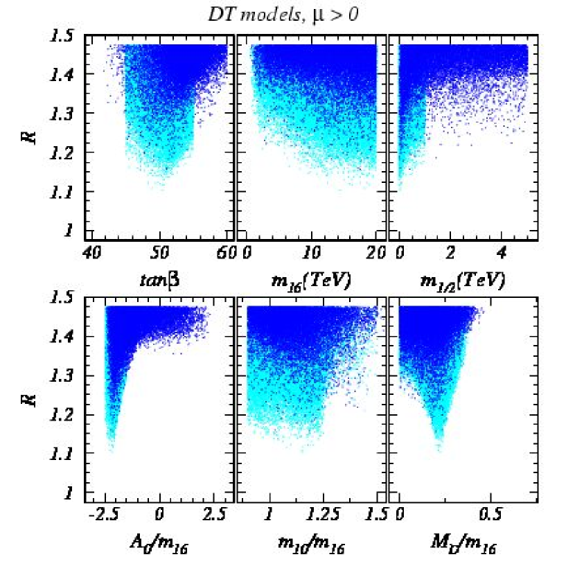
Figure 2: Plot of $R$ versus parameters of the $DT$ model with $\mu>0$ for a) $\tan\beta$, b) $m_{16}$, c) $m_{1/2}$, d) $A_{0}/m_{16}$, e) $m_{10}/m_{16}$ and f) ${\rm sign}(M_{D}^{2})\sqrt{|M_{D}^{2}|}/m_{16}$.

We see that the best Yukawa unification possible gives $R\simeq 1.1$, i.e. Yukawa unification to 10% (really $\pm 5$%). The first three frames show that the best unification occurs for $\tan\beta\sim 50$, and for $m_{16}\stackrel{{\scriptstyle>}}{{\sim}}10$ TeV, and small values of $m_{1/2}\sim 0-0.5$ TeV. We have checked that if we restrict the parameter range to $m_{16}\lesssim 2$ TeV, then $R$ is always larger than 1.25, which is close to the result obtained in Ref. [19]. The fourth frame shows $R$ versus the ratio $A_{0}/m_{16}$. Here we see that the best Yukawa unification occurs sharply next to $A_{0}\sim-2m_{16}$, as in the RIMH scenario, and as in the previous BF analysis. The fifth frame shows $R$ versus the ratio $m_{10}/m_{16}$. Here, the minimum occurs near $m_{10}\sim 1.2m_{16}$, i.e. close to but somewhat below the optimal RIMH value of $m_{10}=\sqrt{2}m_{16}$. Finally, we show $R$ versus the ratio $sign(M_{D}^{2})\sqrt{|M_{D}^{2}|}/m_{16}$. In this case, the best Yukawa unification occurs at $M_{D}\sim 0.25m_{16}$. Choosing $M_{D}=0$ brings us almost back the mSUGRA case (except that $m_{10}$ need not equal $m_{16}$), and the best unification is just $R_{min}=1.28$.

In addition to performing random scans over parameter space, we also scanned for the minimum of $R$ using the MINUIT minimization program. In this case, similar results were obtained, with the minimum occurring for large values of $m_{16}\sim 15$ TeV, and $m_{1/2}\sim 0$.

2.3 $HS$ model

Next, we turn to the $HS$ model. BDR have pointed out that threshold corrections due to the third generation right-handed neutrino (which couples to $H_{u}$ but not $H_{d}$) naturally lead to non-degenerate $m_{H_{u}}^{2}$ and $m_{H_{d}}^{2}$. As in the $DT$ model, the Higgs mass splitting may facilitate REWSB. The difference is that squark and slepton mass parameters are unaffected in the $HS$ model. We adopt the same parameter space as in the $DT$ model, except that this time the splitting applies only to the two Higgs multiplets of the MSSM, while all matter scalars have a common GUT scale mass value given by $m_{16}$.

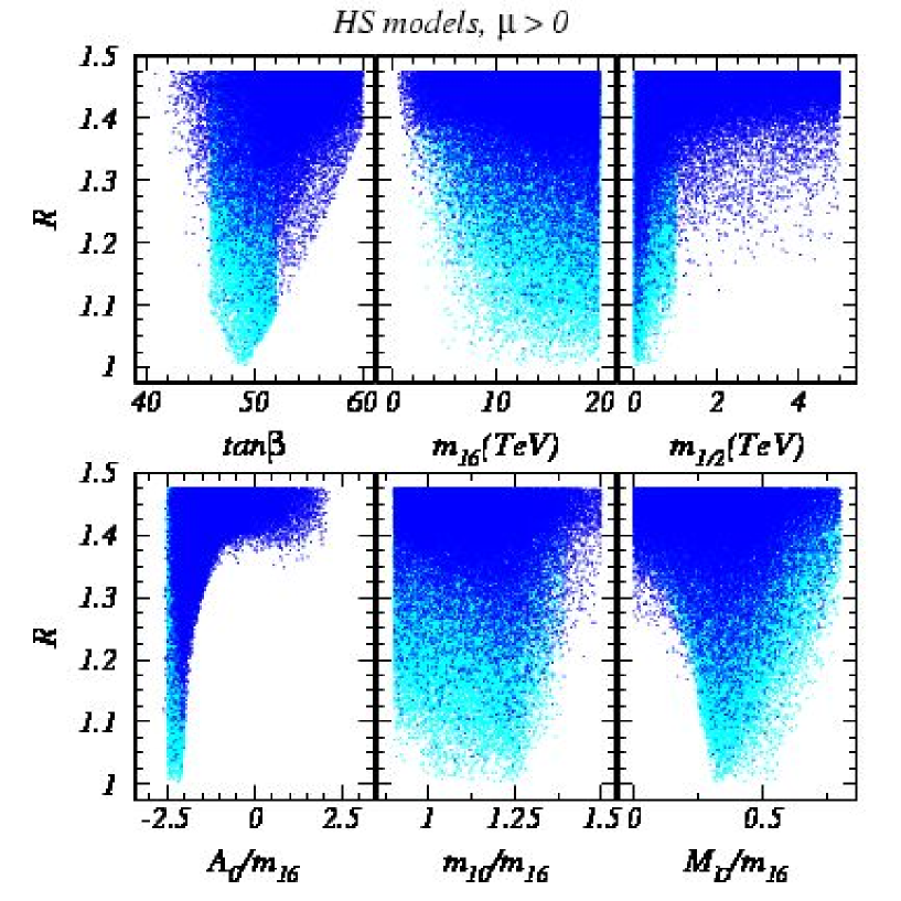
Figure 3: Plot of $R$ versus parameters of the $HS$ model with $\mu>0$ for a) $\tan\beta$, b) $m_{16}$, c) $m_{1/2}$, d) $A_{0}/m_{16}$, e) $m_{10}/m_{16}$ and f) ${\rm sign}(M_{D}^{2})\sqrt{|M_{D}^{2}|}/m_{16}$.

We scan over the same parameter ranges as in the $DT$ model case, with the results shown in Fig. 3 by the dark blue dots. Corresponding results of a more focussed scan over a restricted but optimized range of parameters are shown by the light blue dots. The most noteworthy feature is that we find essentially exact Yukawa coupling unification is possible. The Yukawa unified models are characterized by parameter choices of $\tan\beta\sim 49$, $m_{16}\stackrel{{\scriptstyle>}}{{\sim}}8$ TeV and $m_{1/2}\sim 0-0.4$ TeV, as shown by the first three frames of the figure.

The fourth frame of Fig. 3 shows $R$ versus $A_{0}/m_{16}$, and illustrates the sharp minimum of Yukawa unified models at $A_{0}\sim-(2-2.5)m_{16}$. A choice of $A_{0}\lesssim-2.5m_{16}$ leads to tachyonic masses, while $A_{0}\stackrel{{\scriptstyle>}}{{\sim}}-2m_{16}$ results in much less unified values of Yukawa couplings. The fifth frame shows that Yukawa unification occurs for $m_{10}\sim(1-1.3)m_{16}$, again somewhat lower than the RIMH optimal choice of $m_{10}\simeq\sqrt{2}m_{16}$. The last frame shows $R$ versus ${\rm sign}(M_{D}^{2})\sqrt{|M_{D}^{2}|}/m_{16}$. Here, a somewhat bigger range of $M_{D}^{2}$ (compared to the $DT$ model) yields Yukawa unified solutions which are now obtained for $0.25\lesssim M_{D}/m_{16}\lesssim 0.5$. Reducing the value of $M_{D}$ to zero only allows, at best, solutions with $R$ down to 1.28. In contrast to earlier work on RIMH models, our improved treatment of fermion self-energies in this analysis allows us to find Yukawa unified solutions by accessing much larger values of $m_{16}$ that previously resulted in a breakdown of the REWSB mechanism[23]. We note here that we have performed similar scans using values of $m_{t}=172$ and $180$ GeV (with $m_{b}^{\overline{DR}}(M_{Z})=2.83$ GeV), and $m_{b}^{\overline{DR}}(M_{Z})=3.03$ GeV (with $m_{t}=175$ GeV), and in each case have found results qualitatively similar to those shown in Fig. 3: in particular, $R\simeq 1$ is only obtained for $m_{16}\stackrel{{\scriptstyle>}}{{\sim}}8-10$ TeV

Our next results are shown in Fig. 4. Here, we show the $m_{16}\ vs.\ m_{1/2}$ plane for $m_{10}=1.24m_{16}$, $A_{0}=-2.05m_{16}$, $\tan\beta=49.7$ and $\mu>0$. The mass splitting applied only to the Higgs multiplets is parametrized by $M_{D}=0.334m_{16}$. The contours show regions where $R<1.03$ and $R<1.02$, i.e. Yukawa unification to better than 2-3%. As seen from the figure, these regions occur at extremely large values of $m_{16}\simeq 8-20$ TeV. Since scalar masses are so large, it is critical to perform coupling constant and soft term mass evolution using two-loop RGEs[32]. The resulting first and second generation multi-TeV scalar masses are sufficient to suppress most SUSY flavor and $CP$ violating processes, and offers a decoupling solution to the SUSY flavor and $CP$ problems. This comes at some fine-tuning expense, since third generation scalars, while suppressed, typically have masses in the few TeV range.

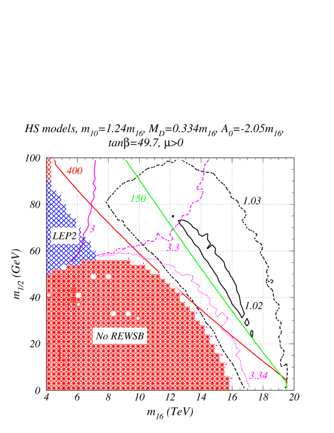
Figure 4: A plot in the $m_{16}\ vs.\ m_{1/2}$ plane for $\tan\beta=49.7$, showing contours of Yukawa unification parameter $R$ (black), contours of $BF(b\rightarrow s\gamma)$ ($\times 10^{4}$) (magenta), and contours of $m_{\tilde{g}}=400$ GeV (red) and $m_{\widetilde{W}_{1}}=150$ GeV (green).

A characteristic feature of these solutions is that $m_{1/2}$ is rather small, typically less than $150$ GeV, giving rise to relatively light masses for the $\tilde{g}$ and lighter charginos and neutralinos. Also shown in Fig. 4 are contours of $m_{\tilde{g}}=400$ GeV and $m_{\widetilde{W}_{1}}=150$ GeV. The former may just be accessible to Fermilab Tevatron searches for $\tilde{g}\tilde{g}$ production with large values of $m_{\tilde{q}}$[33], while the latter may be accessible via $\widetilde{W}_{1}\widetilde{Z}_{2}\rightarrow 3\ell$ searches[34, 35].

Representative examples of sample solutions are shown in Table 1, with $m_{16}$ values of $2.5,\ 5.31,\ 10$ and $14$ TeV, and also a small $\mu$ point with $m_{16}=1500$ GeV (pt. 5) that we will discuss separately. We list the GUT scale values of the three Yukawa couplings, plus a variety of physical SUSY particle masses. In particular, $m_{\tilde{t}_{1}}$ varies from $0.24-3.3$ TeV for these solutions. We also list the “crunch factor” $S$ as defined in Ref. [22, 23]:

$$S={{3(m_{\tilde{u}_{L}}^{2}+m_{\tilde{d}_{L}}^{2}+m_{\tilde{u}_{R}}^{2}+m_{\tilde{d}_{R}}^{2})+m_{\tilde{e}_{L}}^{2}+m_{\tilde{e}_{R}}^{2}+m_{\tilde{\nu}_{e}}^{2}}\over{3(m_{\tilde{t}_{1}}^{2}+m_{\tilde{b}_{1}}^{2}+m_{\tilde{t}_{2}}^{2}+m_{\tilde{b}_{2}}^{2})+m_{\tilde{\tau}_{1}}^{2}+m_{\tilde{\tau}_{2}}^{2}+m_{\tilde{\nu}_{\tau}}^{2}}}.$$ (6)

We see that the solutions typically have $S\sim 6-7$, in accord with previous results from Ref. [23], but lower than those generated by the approximate analytic calculations in Ref. [22].

Pt. 5 in Table 1 has been chosen to try to duplicate the first point in Table 1 of BDR, and to show that we are able to find solutions with a small values of $\mu$. The only difference in input parameters from BDR is that we take $m_{10}/m_{16}=1.315$ instead of 1.35, so that REWSB is satisfied in ISAJET. We differ from BDR in that for solutions with small $\mu$, we are unable to obtain $R$ smaller than about 1.2. Pt. 5 (or a variant thereof) which is unequivocally excluded by the very large value for $BF(b\rightarrow s\gamma)$, would otherwise be quite acceptable on phenomenological grounds. The higgsino component of the neutralino allows efficient annihilation of cosmological LSPs, resulting in too low a relic density to account for all dark matter. The value of $BF(B_{s}\rightarrow\mu^{+}\mu^{-})$ appears to be within reach of Run 2 of the Tevatron. Indeed the Tevatron may be able to directly discover charginos and neutralinos via trilepton searches, while a plethora of signals should be observable at the LHC. However, since this point is excluded we will not refer to it any further.

Table 1: Model parameters, Yukawa couplings and corresponding sparticle masses for five case studies in the $HS$ model with $\mu>0$.

parameter	pt. 1	pt. 2	pt. 3	pt. 4	pt. 5
$m_{16}$	2493.0	5310.0	10000.0	14000.0	1500
$m_{10}$	3226.0	6595.0	12420.0	17360.0	1972.5
$M_{D}$	975.0	1778.8	3350.0	4676.0	502.9
$m_{1/2}$	130.0	79.0	79.0	65.0	250
$A_{0}$	-4754.0	-10885.5	-20500.0	-28700.0	-2745.0
$\tan\beta$	50.6	49.7	49.7	49.7	51.2
$f_{t}(M_{GUT})$	0.507	0.537	0.557	0.560	.507
$f_{b}(M_{GUT})$	0.453	0.536	0.559	0.560	0.455
$f_{\tau}(M_{GUT})$	0.539	0.561	0.571	0.571	0.558
$\epsilon_{3}=\frac{\alpha_{3}(M_{GUT})-\alpha_{GUT})}{\alpha_{GUT}}$	-0.034	-0.025	-0.019	-0.015	-0.042
$R$	1.19	1.05	1.03	1.02	1.23
$m_{\tilde{g}}$	434.3	366.4	456.0	486.1	681.2
$m_{\tilde{u}_{L}}$	2462.7	5225.2	9849.8	13796.0	1554.1
$m_{\tilde{d}_{R}}$	2479.3	5255.8	9905.0	13871.6	1557.1
$m_{\tilde{t}_{1}}$	418.4	1042.1	2244.0	3335.8	235.1
$m_{\tilde{b}_{1}}$	820.2	1520.2	2946.4	4274.2	587.9
$m_{\tilde{\ell}_{L}}$	2463.6	5257.7	9904.1	13868.0	1494.2
$m_{\tilde{\ell}_{R}}$	2463.6	5358.8	10090.1	14124.1	1517.6
$m_{\tilde{\nu}_{e}}$	2527.2	5257.1	9903.7	13867.7	1492.0
$m_{\tilde{\tau}_{1}}$	909.0	2095.8	4069.0	5790.1	498.9
$m_{\tilde{\nu}_{\tau}}$	1825.8	3960.1	7496.0	10524.0	1104.1
$m_{\widetilde{W}_{1}}$	110.9	104.1	141.0	159.9	129.7
$m_{\widetilde{Z}_{2}}$	110.9	104.0	140.9	159.7	140.2
$m_{\widetilde{Z}_{1}}$	58.4	49.3	64.8	71.7	90.3
$m_{h}$	125.6	127.9	130.7	131.4	121.0
$m_{A}$	1168.6	1018.0	1841.2	2733.2	525.7
$m_{H^{+}}$	1174.1	1024.1	1845.5	2737.1	536.3
$\mu$	303.8	1404.5	2533.7	3480.3	160.5
$S$	5.94	6.53	6.37	6.16	5.26
$a_{\mu}\times 10^{10}$	3.81	0.362	0.0841	0.0373	11.05
$BF(b\rightarrow s\gamma)\times 10^{4}$	2.83	2.54	3.23	3.32	70.9
$BF(B_{s}\rightarrow\mu^{+}\mu^{-})\times 10^{8}$	1.37	2.89	0.937	0.610	11.5
$\Omega_{\widetilde{Z}_{1}}h^{2}$	0.178	180.	50.4	32900	0.054

In Fig. 5, we show the evolution of gauge and Yukawa couplings (upper frame), and soft SUSY breaking parameters (lower frame), versus the renormalization scale $Q$. The example point has $m_{16}=10$ TeV, and corresponds to pt. 3 in Table 1. The separate gauge and Yukawa coupling unifications at $Q=M_{GUT}$ are evident in the upper frame. In the lower frame, the evolution characteristic to the RIMH framework shows the suppression of third generation and Higgs soft breaking parameters relative to those of the first or second generation.

Figure 5: Gauge and Yukawa coupling evolution (upper frame) and the evolution of select soft SUSY breaking parameters (lower frame) versus scale $Q$ for the case study pt. 3 with $m_{16}=10$ TeV. The unification of the three gauge couplings, and independently, of the three Yukawa couplings is illustrated.

In Fig. 6, we show selected sparticle mass spectra versus $m_{16}$ obtained for $\tan\beta=50.6$, $m_{1/2}=100$ GeV, $m_{10}=1.24m_{16}$, $M_{D}=0.321m_{16}$ and $A_{0}=-2m_{16}$. The considerable gap between first and third generation sparticle masses is prominently displayed. As already discussed, the gap has a dynamical origin, and may solve the SUSY flavor and $CP$ problems via a decoupling solution while maintaining naturalness.

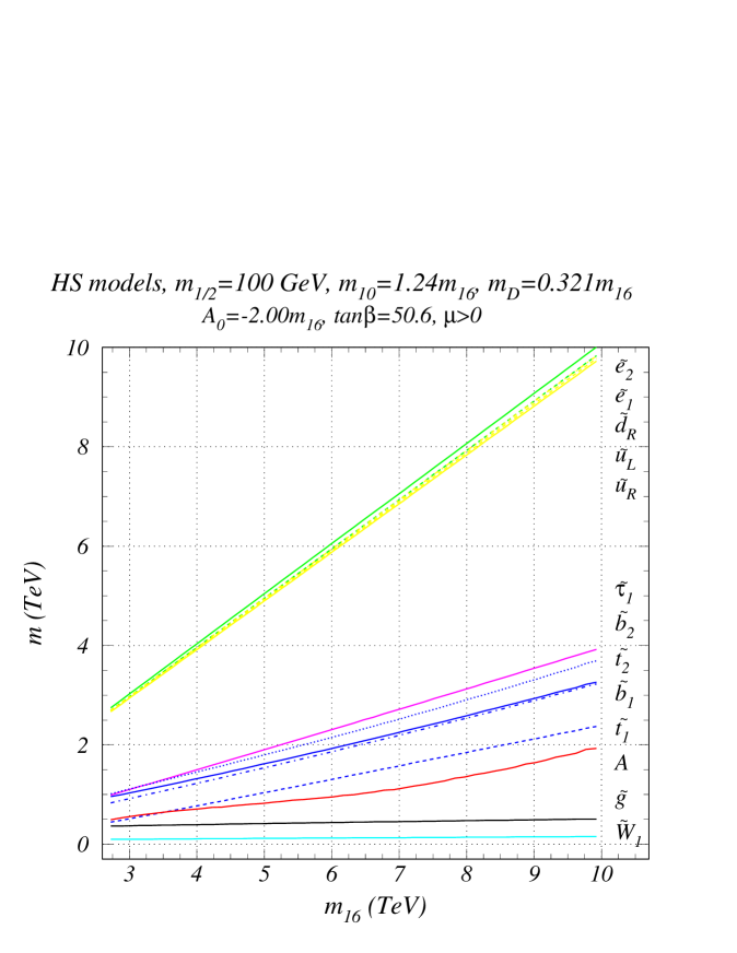
Figure 6: Selected sparticle masses versus $m_{16}$ for $m_{1/2}=100$ GeV and other parameters as listed on the figure.

In Table 1, we also list the corresponding values of $a_{\mu}$[36], $BF(b\rightarrow s\gamma)$[37], $BF(B_{s}\rightarrow\mu^{+}\mu^{-})$[38] and $\Omega_{\widetilde{Z}_{1}}h^{2}$[39]. Many authors have evaluated these quantities within SUSY models: above, we cite the paper whose calculation we have used to obtain the results shown here. Contours for these observables are also shown in Fig. 7, for the value of $\tan\beta=50.6$. The color characterizes the observable, and for each observable, the contour type (solid or dashed) characterizes a value for the observable. Also shown are regions excluded by various theoretical (no or improper REWSB) and experimental constraints from LEP2. In the region labelled, “No RGE convergence”, the solutions to the renormalization group equation do not satisfy the convergence criteria required in ISAJET. The value of $BF(b\rightarrow s\gamma)$ is below the averaged measured value of $BF(b\rightarrow s\gamma)=(3.25\pm 0.37)\times 10^{-4}$ for pt. 2, but in closer accord with experiment for pts. 1, 3 and 4; however, the prediction for the first four points is compatible with the experimental value once theoretical unceertainties are taken into account. This is unlike the case of Yukawa unified models with $\mu<0$, which typically yield too large a value of $BF(b\rightarrow s\gamma)$. The value of $a_{\mu}$ is rather small for all points due to suppression from the multi-TeV smuon and sneutrino masses, but is not inconsistent with measurements from experiment $E821$. Also, the CDF collaboration has found $BF(B_{s}\rightarrow\mu^{+}\mu^{-})<2.6\times 10^{-6}$, and expects to probe to about $10^{-7}$ with Run 2 data. Points 1-4 are likely out-of-reach for the Tevatron $BF(B_{S}\rightarrow\mu^{+}\mu^{-})$ measurements, but they will be probed at the LHC after about two years of operation.

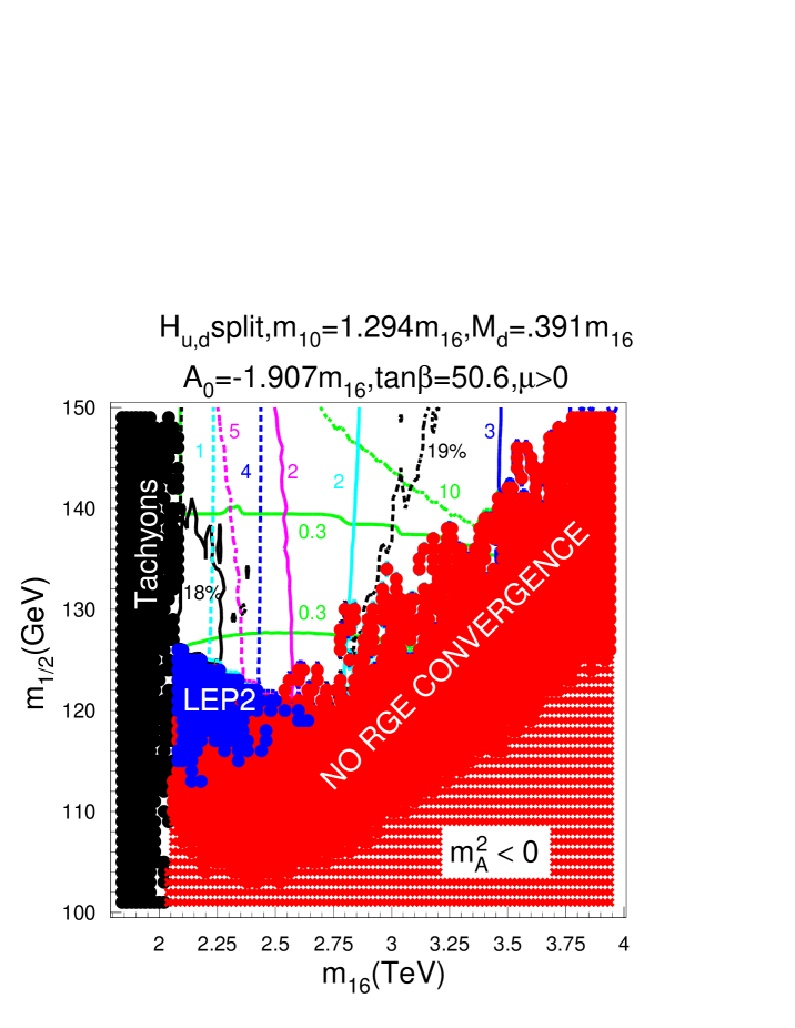
Figure 7: A plot of the $m_{16}\ vs.\ m_{1/2}$ plane, illustrating contours of Yukawa unification parameter R(black), $BF(b\rightarrow s\gamma)(\times 10^{4})$ (magenta), $a_{\mu}(\times 10^{10})$ (blue), $BF(B_{s}\rightarrow\mu^{+}\mu^{-})(\times 10^{8})$ (light blue) and $\Omega_{\widetilde{Z}_{1}}h^{2}$ (green).

Phenomenologically, the most problematic is the value of the neutralino relic density $\Omega_{\widetilde{Z}_{1}}h^{2}$. For pt. 1, $\Omega_{\widetilde{Z}_{1}}h^{2}$ is in the observationally acceptable range $\Omega_{CDM}=0.1-0.3$ because of resonance annihilation via $\widetilde{Z}_{1}\widetilde{Z}_{1}\rightarrow h\rightarrow b\bar{b}$ in the early universe. Annihilation via $t$ and $u$ channel sfermion exchange is also significant. As $m_{16}$ increases (pts. 2-4), these other annihilation channels are increasingly suppressed. Furthermore, for these points, $2m_{\widetilde{Z}_{1}}>m_{h}$ so that annihilation via $s$-channel $h$ is no longer resonant. As a result, the neutralino relic density is very high. There is, therefore, considerable tension between the theoretical requirement of a high degree of Yukawa coupling unification, and the phenomenological requirement that the age of the universe is greater than 10 Gyr. There seems to be little overlap of parameter regions consistent with both requirements for these $\mu>0$ solutions. (In the case of $\mu<0$, a reasonable relic density can be obtained by large rates for $\widetilde{Z}_{1}\widetilde{Z}_{1}\rightarrow A,\ H\rightarrow b\bar{b}$ in the early universe[16], but then the problem is with the $b\rightarrow s\gamma$ decay rate.)

It is well known that the relic density can be low in the “focus point” region of the mSUGRA model[41]. The focus point region occurs near the upper boundary of the common scalar mass $m_{0}$, which is determined by where $\mu^{2}\rightarrow$ negative values, thus signaling a breakdown in REWSB. Since $|\mu|$ is small, the $\widetilde{Z}_{1}$ has a significant higgsino component, and there is large annihilation to states such as $WW$ or $ZZ$, and possibly even co-annihilation if $m_{\widetilde{W}_{1}}\simeq m_{\widetilde{Z}_{1}}$. A possible solution to the too-high relic density problem is to try to dial in lower Higgs mass splittings. This should make the model more mSUGRA-like, and bring back the focus-point region. We have checked this, but found that increasing the higgsino component of the lighter charginos and neutralinos also modifies the $b$ and $t$ quark threshold corrections so that Yukawa unification can reach only values of $R=1.2-1.3$.

The other option to lower the relic density is to find a region with neutralino annihilation via the light Higgs boson. Such an example is presented by point 1 of Table 1 and illustrated in Fig. 7. One can clearly see a corridor in $m_{1/2}$ of $\sim 15$ GeV width where annihilation through the the light Higgs boson occurs. Part of this corridor satisfies all experimental constraints but Yukawa unification reaches only 19% here.

3 Supersymmetric models with $\mu<0$

Next, we turn to the re-examination of Yukawa unification for models with $\mu<0$. Our goal is to update our earlier results[14, 16], which found Yukawa unification to be possible for a range of parameters within the $DT$ model.

3.1 mSUGRA model

Again, we begin by examining Yukawa unification within the mSUGRA model. As before, we scan over the four mSUGRA model parameters, and plot the value of $R$ against each of them. Our results are shown in Fig. 8.

Figure 8: Plot of Yukawa unification parameter $R$ versus input parameters of the mSUGRA model for a) $m_{0}$, b) $m_{1/2}$, c) $A_{0}$ and d) $\tan\beta$, when $\mu<0$.

The results of these scans show that Yukawa unification to $R\sim 1.15-1.20$ can be achieved if $m_{0},\ m_{1/2}\lesssim 1$ TeV. But as model parameters increase, the Yukawa unification improves, and is reaching the 5–10% level for $m_{1/2}\sim 5$ TeV and $\tan\beta\sim 55$. To see whether unification is possible for yet larger values of sparticle masses, we continued these scans out to even higher values of model parameters. We found that Yukawa unification is possible within the mSUGRA model for $m_{0}$ values around 10 TeV, and $m_{1/2}\sim 1.6m_{0}$. Our results for the extended mSUGRA parameter space illustrating this are shown in Fig. 9.

Figure 9: Plot of Yukawa unification parameter $R$ versus input parameters of the mSUGRA model, a) $m_{0}$, b) $m_{1/2}$, c) $A_{0}/m_{0}$ and d) $\tan\beta$, when $\mu<0$ and extended ranges of these parameters.

A particular case is shown as point 1 in Table 2, which has Yukawa unification to 1%. In this case, squarks and sleptons have mass values of 10–30 TeV (including third generation sparticles), and the models suffer from the need for fine-tuning. The models are in the decoupling regime, so that the values of $a_{\mu}$ and $BF(b\rightarrow s\gamma)$ will be near the SM predicted values. However, the neutralino relic density is extremely high ($\Omega h^{2}=52.6$ for the model listed in the table), so that $R$-parity violation would be needed to make the model cosmologically viable. Of course, we would then need another candidate for dark matter.

Table 2: Model parameters, Yukawa couplings and weak scale sparticle masses for four case studies for $\mu<0$.

	1	2	3	4	5
parameter	mSUGRA	$DT_{1}$	$DT(f_{\nu})$	$DT_{2}$	$HS$
$m_{16}$	9616.1	1000.0	1000.0	2775.8	2000.0
$m_{10}$	9616.1	1414.0	1414.0	3763.6	2709.4
$M_{D}$	0.0	333.0	333.0	1095.0	1048.4
$m_{1/2}$	14893.2	700.0	700.0	2033.6	1500.0
$A_{0}$	-7943.8	0.0	0.0	0.0	-560.2
$\tan\beta$	56.29	54.0	54.0	56.0	54.8
$M_{N}$	$M_{GUT}$	$M_{GUT}$	$1.0\times 10^{15}$	$M_{GUT}$	$M_{GUT}$
$f_{t}(M_{GUT})$	0.610	0.599	0.609	0.611	0.608
$f_{b}(M_{GUT})$	0.606	0.556	0.580	0.614	0.616
$f_{\tau}(M_{GUT})$	0.609	0.572	0.582	0.616	0.609
$R$	1.01	1.08	1.05	1.01	1.01
$m_{\tilde{g}}$	27536.5	1602.2	1600.9	4319.5	3241.9
$m_{\tilde{u}_{L}}$	24898.2	1697.2	1696.5	4641.9	3355.9
$m_{\tilde{d}_{R}}$	23573.9	1518.1	1517.8	3960.2	3237.2
$m_{\tilde{t}_{1}}$	19073.3	1166.2	1169.1	3304.4	2388.5
$m_{\tilde{b}_{1}}$	19381.7	1083.6	1069.1	2704.3	2328.8
$m_{\tilde{\ell}_{L}}$	13292.6	928.5	928.5	2376.3	2192.2
$m_{\tilde{\ell}_{R}}$	10981.9	1094.4	1094.4	3108.4	2121.3
$m_{\tilde{\nu}_{e}}$	13292.4	925.1	925.0	2375.0	2190.7
$m_{\tilde{\tau}_{1}}$	7843.1	715.2	694.6	1795.7	1268.6
$m_{\tilde{\nu}_{\tau}}$	12166.8	734.6	704.9	1796.8	1839.3
$m_{\widetilde{W}_{1}}$	12415.4	419.4	448.1	1344.7	1179.8
$m_{\widetilde{Z}_{2}}$	12415.3	422.3	449.9	1345.5	1309.9
$m_{\widetilde{Z}_{1}}$	7143.9	288.4	290.0	894.5	654.0
$m_{h}$	127.6	120.0	120.0	123.9	123.5
$m_{A}$	1854.8	624.3	614.9	1864.4	1384.0
$m_{H^{+}}$	1859.2	632.9	623.6	1868.7	1388.9
$\mu$	-12943.7	-438.1	-472.7	-1353.7	-1277.5
$S$	1.46	1.80	1.81	1.80	1.79
$a_{\mu}\times 10^{10}$	-0.0453	-40.8	-40.0	-10.3	-2.76
$BF(b\rightarrow s\gamma)\times 10^{4}$	3.52	7.35	7.40	4.08	4.47
$BF(B_{s}\rightarrow\mu^{+}\mu^{-})\times 10^{8}$	0.198	0.273	0.300	0.315	0.223
$\Omega_{\widetilde{Z}_{1}}h^{2}$	52.6	0.00854	0.00683	0.251	0.294

3.2 $DT$ model

Next, we re-examine Yukawa coupling unification in the $DT$ model with $\mu<0$. We scan over similar ranges of model parameters as in the $\mu>0$ case, and plot the value of $R$ versus model parameters in Fig. 10. As for the mSUGRA model just discussed, we find that a high degree of Yukawa coupling unification is possible for $\tan\beta\sim 55$. However, in contrast to the mSUGRA model case, we can now achieve Yukawa coupling unification even for $m_{16}$ values of 1 TeV, or smaller. Yukawa unified models prefer large values of $m_{1/2}$, typically greater than a TeV. Unlike the Yukawa unified models with $\mu>0$, a wide range of ratios of $A_{0}/m_{16}$ are allowed, centered about $A_{0}\sim 0$. Moreover, the parameter $m_{10}$ can be greater than or less than $m_{16}$. The final frame of Fig. 10 shows that a positive $D$-term $M_{D}/m_{16}\sim 0.2-0.4$ is required for a high degree of Yukawa coupling unification. The need for the $D$-term is lessened as we increase the range of model parameters, the limiting case being the previously shown mSUGRA model.

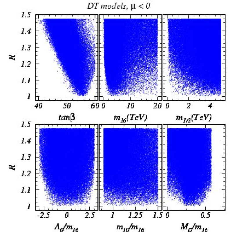
Figure 10: Plot of $R$ versus parameters of the $DT$ model with $\mu<0$ for a) $\tan\beta$, b) $m_{16}$, c) $m_{1/2}$, d) $A_{0}/m_{16}$, e) $m_{10}/m_{16}$ and f) ${\rm sign}(M_{D}^{2})\sqrt{|M_{D}^{2}|}/m_{16}$.

In Fig. 11, we show contours for the same observables as in Fig. 7 along with contours of $R$ in the $m_{16}\ vs.\ m_{1/2}$ plane for $\tan\beta$ values of $52,\ 54,\ 56$ and $58$. The legends for the various contours are shown on the figure. We take $m_{10}=1.414m_{16}$, $M_{D}=0.333m_{16}$ and $A_{0}=0$. In the figures, the low $m_{16}$ regions of parameter space are excluded by the requirement $m_{\tilde{\tau}_{1}}>m_{\widetilde{Z}_{1}}$. As $\tan\beta$ increases, this excluded region is usurped by the requirement that $m_{A}^{2}>0$, which increasingly excludes the parameter plane denoted by asterisks. In the large $m_{16}$ and low $m_{1/2}$ regions, parameter space is forbidden because $\mu^{2}<0$ (pluses), which signals a breakdown in REWSB. Thus, the allowed parameter space turns out to be a narrow wedge between these two extremes, and is increasingly restricted as $\tan\beta$ increases.

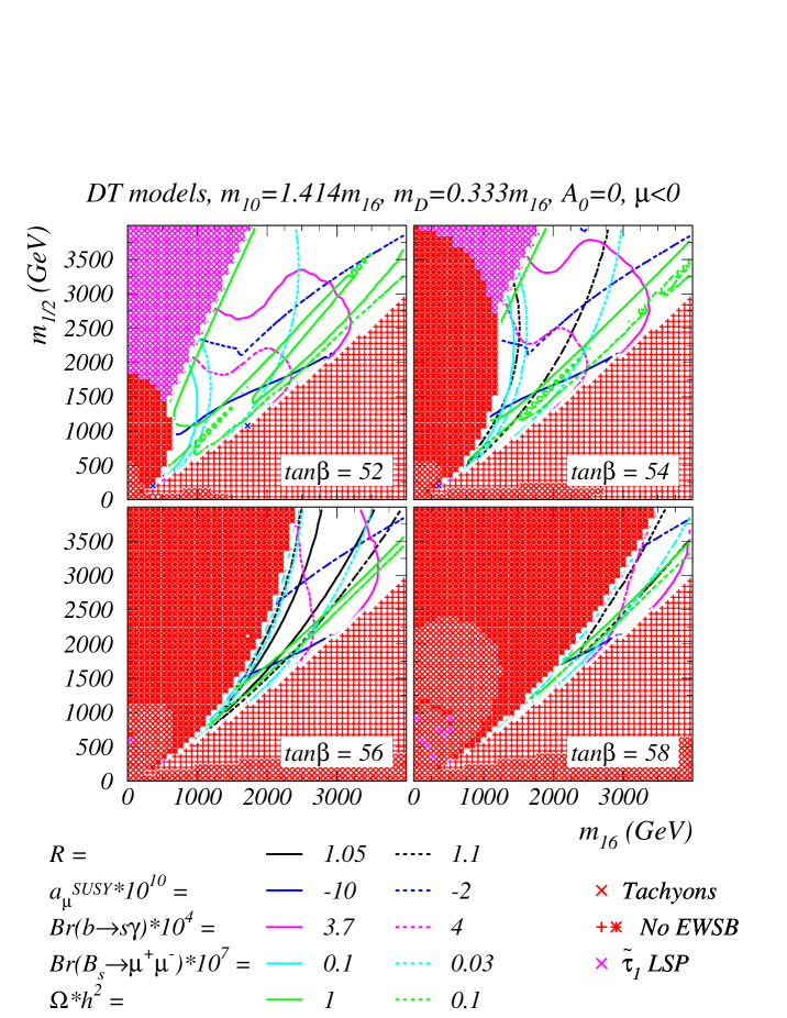
Figure 11: Contours of $R$ together with those of selected observables in $m_{16}\ vs.\ m_{1/2}$ plane for various $\tan\beta$ values, with $\mu<0$ and $A_{0}=0$ for the $DT$ model.

In the theoretically allowed regions, the solid and dotted black contours show regions where $R<1.05$ and 1.10, respectively. The largest Yukawa unified regions occur in the third frame, where $\tan\beta=56$. In between the solid (dashed) lines for this case, $R<1.05$ (1.1). In the neighbouring cases with $\tan\beta=54$ and $\tan\beta=58$, no solid black line appears because $R>1.05$, while in the first frame $R>1.1$. We also show contours of values of $a_{\mu}$, $BF(b\rightarrow s\gamma)$, $BF(B_{S}\rightarrow\mu^{+}\mu^{-})$ and $\Omega_{\widetilde{Z}_{1}}h^{2}$. The $a_{\mu}$ values are always negative, and so disfavored by recent results from the E821 experiment. However, for large values of model parameters, $a_{\mu}$ approaches its SM value, and lies at least within $3\sigma$ of the experimental result (the exact deviation depends upon which SM $a_{\mu}$ calculation is adopted). Even more problematic is the value of $BF(b\rightarrow s\gamma)$, which is above $4\times 10^{-4}$ below the dashed magenta contours. Requiring consistency of the models with $BF(b\rightarrow s\gamma)$ pushes model parameters to very high values. Contours of $BF(B_{s}\rightarrow\mu^{+}\mu^{-})=0.1\times 10^{-7}$ and $0.03\times 10^{-7}$ are also shown; this branching fraction seems somewhat out of reach of the CDF experiment.

The values $\Omega_{\widetilde{Z}_{1}}h^{2}=0.1$ and 1 are also shown by the green dashed and solid contours. In the frames shown, a reasonable relic density is obtained in three distinct regions.

1. Near the boundary of the low $m_{16}$ excluded region (shown by magenta x’s) for $\tan\beta=52$ and 54, $m_{\tilde{\tau}_{1}}\simeq m_{\widetilde{Z}_{1}}$ and $\tilde{\tau}_{1}-\widetilde{Z}_{1}$ and $\tilde{\tau}_{1}-\tilde{\tau}_{1}$ co-annihilation reduces the relic density to reasonable values[42].

2. Near the boundary of large $m_{16}$, where $|\mu|$ becomes small, the higgsino component of $\widetilde{Z}_{1}$ increases, so that there is efficient $\widetilde{Z}_{1}-\widetilde{Z}_{1}$ annihilation into vector boson pairs.

3. In the first three frames, a corridor of resonance annihilation $\widetilde{Z}_{1}\widetilde{Z}_{1}\rightarrow A,\ H\rightarrow b\bar{b},\ \tau\bar{\tau}$ occurs, which severely lowers the relic density[43].

Simultaneously fulfilling all three constraints, $a_{\mu}$, $BF(b\rightarrow s\gamma)$ and $\Omega h^{2}$, plus obtaining a high degree of Yukawa coupling unification is challenging–but possible–and depends upon the tolerances required of each constraint.

As an example, we show point 2 in Table 2, with good Yukawa unification and relatively low values of soft SUSY breaking model parameters. For this point, third generation squark masses are in the 1-2 TeV range, so there should not be too much fine tuning required. The sparticle mass spectrum is rather heavy, and other than possibly the light boson Higgs $h$, none of the new states would be accessible to Tevatron SUSY searches. Sparticles should be accessible to LHC SUSY searches, but would be inaccessible at 500 GeV linear colliders (except for the Higgs $h$). As the machine energy is increased, $\widetilde{Z}_{1}\widetilde{Z}_{2}$ production would be accessible for $\sqrt{s}\stackrel{{\scriptstyle>}}{{\sim}}750$ GeV, and chargino pair production would become accessible for $\sqrt{s}\stackrel{{\scriptstyle>}}{{\sim}}850$ GeV. The value of $m_{\widetilde{Z}_{1}}\simeq m_{A}/2$ (given the broad width of the $A$ and $H$), so that efficient $s$-channel annihilation of neutralinos can take place in the early universe, and a very low relic density is generated. However, the values of $a_{\mu}$ and $BF(b\rightarrow s\gamma)$ are well beyond their experimental limits, so that the point is likely excluded.

The third point in Table 2 shows the same parameter space point, except that the MSSM is enlarged to include a gauge singlet chiral scalar superfield $\hat{N}_{i}^{c}$ for each generation $i=1-3$, and which contains a right-handed neutrino as its fermionic component. The superpotential is enlarged to include the terms

$$\hat{f}\ni{1\over 2}M_{N}\hat{N}^{c}\hat{N}^{c}+f_{\nu}\epsilon_{ij}\hat{L}^{i}\hat{H}_{u}^{j}\hat{N}^{c}$$ (7)

for each generation. We retain only the third generation Yukawa coupling which we assume satisfies $f_{\nu_{\tau}}=f_{t}$ at $Q=M_{GUT}\simeq 2\times 10^{16}$ GeV, and take $M_{N}=1\times 10^{15}$ GeV. This value of $M_{N}$ gives a $\nu_{\tau}$ mass in accord with atmospheric neutrino measurements at the SuperK experiment. The neutrino Yukawa coupling is coupled through the RGEs with the other Yukawa couplings and soft SUSY breaking parameters, but decouples below the scale $M_{N}$. Its effect, in this case, is to improve Yukawa coupling unification from $R=1.08$ to $R=1.05$. In addition, the third generation neutrino Yukawa coupling acts to somewhat suppress the third generation slepton and sneutrino masses.

We found that it is possible to reasonably satisfy the indirect experimental constraints while obtaining good Yukawa unification in the $DT$ model provided that the input parameters with mass dimensions are increased. This is illustrated by point 4 of Table 2. Since $m_{16}$ and $m_{1/2}$ (and proportionally $m_{10}$ and $M_{D}$) are somewhat higher than in point 2, the mass spectrum is heavier and only the lightest Higgs particle is detectable at the Tevatron or the LC. But the Yukawa unification is perfect and the neutralino relic density is ideal. The values of $a_{\mu}$ and $BF(b\rightarrow s\gamma)$ comply substantially better with the experiments than those of point 2 or 3, due to the heaviness of superpartners in the relevant loops. Unfortunately, direct detection of sparticles will be difficult even at the LHC.

3.3 $HS$ model

We also investigate Yukawa coupling unification for $\mu<0$ in the $HS$ model. We scan over parameter space exactly as in the $DT$ model, except that mass splittings are only applied to the Higgs multiplets. The results of $R$ versus various model parameters are shown in Fig. 12. We find that Yukawa coupling unification is again possible below the 1% level for a wide range of model parameters. In fact, the results are qualitatively quite similar to the case of the $DT$ model for $\mu<0$. The best unification occurs at $\tan\beta\sim 55$. The main difference is that a wider range of $D$-terms is now allowed. This, it has been pointed out[18], is because in the $HS$ scenario sfermion masses and hence the corrections to $m_{b}$ are not altered by the splitting: in contrast, in the $DT$ scenario, $m_{\tilde{b}_{R}}^{2}$ is reduced by positive $D$-terms, resulting in an enhancement of the gluino contribution to $\delta m_{b}$.

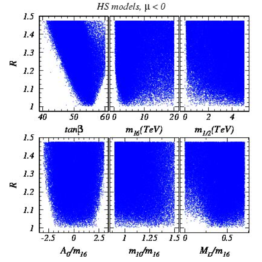
Figure 12: The unification parameter $R$ versus parameters a) $\tan\beta$, b) $m_{16}$, c) $m_{1/2}$, d) $A_{0}/m_{16}$, e) $m_{10}/m_{16}$ and f) ${\rm sign}(M_{D}^{2})\sqrt{|M_{D}^{2}|}/m_{16}$ of the $DT$ model, for $\mu<0$.

In Fig. 13, we show the same $m_{16}\ vs.\ m_{1/2}$ plane plots as in Fig. 11, but for the $HS$ model. Again, we show contours of Yukawa coupling unification parameter $R$, $a_{\mu}$, $BF(b\rightarrow s\gamma)$, $BF(B_{s}\rightarrow\mu^{+}\mu^{-})$ and $\Omega_{\widetilde{Z}_{1}}h^{2}$. The results are qualitatively very similar to those of the $DT$ model, except that the Yukawa coupling unification is marginally worse, and the allowed range of parameters is slightly reduced.

We show point 5 in Table 2 as an example of an $HS$ model. This model point also features more massive sparticles than points 2 and 3, and is inaccessible at the Tevatron, and probably, even at the LHC. This point has essentially perfect Yukawa unification and satisfies all the experimental data within experimental and theoretical errors.

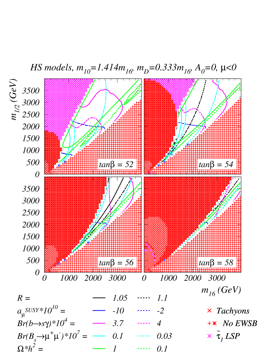
Figure 13: Plot of $m_{16}\ vs.\ m_{1/2}$ plane for various $\tan\beta$ values, $\mu<0$ and $A_{0}=0$.

4 Comparison with BDR results

As we have already discussed, a similar analysis to the one in this paper has been performed by Blazek, Dermisek and Raby (BDR)[18] for the case of $\mu>0$. The results of BDR have many similarities, but also important differences, to our results and to the results in Ref. [19]. In this section, we first compare our calculational procedure based on ISAJET with that of BDR. Next, we comment on similarities and differences in numerical results. Finally, in the last section, we present some general remarks about our program of calculations.

4.1 Comparison of the top–down versus bottom–up procedures

BDR adopt a top-down approach to calculating the sparticles mass spectrum. They begin with the parameters,

$$M_{GUT},\ \alpha_{GUT},\ \epsilon_{3},\ \lambda,\ \mu,\ m_{1/2},\ A_{0},\ \tan\beta,\ m_{16}^{2},\ m_{10}^{2},\ \Delta m_{H}^{2},$$ (8)

where $\epsilon_{3}$ parameterizes the small $GUT$ scale non-unification of the $SU(3)_{C}$ gauge coupling with the electroweak gauge couplings ($\epsilon_{3}=(\alpha_{3}(M_{GUT})-\alpha_{GUT})/\alpha_{GUT}$), $\lambda$ is the unified third generation Yukawa coupling, $\Delta m_{H}^{2}$ represents the Higgs mass squared splitting (about $m_{10}^{2}$) in the $HS$ model (equal to $M_{D}^{2}$ in the $DT$ model), and the other parameters are as in this paper. They evolve via two-loop RGEs for dimensionless parameters and one-loop RGEs for dimensionful parameters via MSSM RGEs to the scale $Q=M_{Z}$, where REWSB is imposed assuming the radiatively corrected scalar potential of a two-Higgs doublet model with softly broken supersymmetry. At $Q=M_{Z}$, they evaluate the 9 observables: $\alpha_{EM}$, $G_{\mu}$, $\alpha_{s}(M_{Z}^{2})$, $M_{Z}$, $M_{W}$, $\rho_{NEW}$, $m_{t}$, $m_{b}^{\overline{MS}}(m_{b})$ and $m_{\tau}$, all including one-loop radiative corrections. In particular, the SUSY threshold corrections to $m_{t}$, $m_{b}$ and $m_{\tau}$ are all calculated and imposed at scale $Q=M_{Z}$. Also, the spectrum of SUSY and Higgs particles is calculated. Radiative corrections are included for the various Higgs masses $m_{h}$, $m_{H}$ and $m_{A}$, while SUSY particle masses are taken to be running mass parameters evaluated at $Q=M_{Z}$. Next, the experimental values for these observables together with the associated errors are used to obtain $\chi^{2}$ for each set of inputs, and this $\chi^{2}$ is minimized using the CERN program MINUIT. Thus, by scanning over the 11-dimensional GUT scale parameter space, they search for parameter regions leading to good agreement with the 9 observables. In particular, their third generation Yukawa couplings are always truly unified. In general, the electroweak observables and the third generation fermion masses will deviate from their measured central values. BDR seek input parameter choices which minimize the overall deviation, and result in acceptable values of $\chi^{2}$.

We use ISAJET, where an iterative, bottom-up approach is adopted. The calculation begins by inputting at scale $Q=M_{Z}$ the $\overline{DR}$ central values of the three gauge couplings $g_{1}$, $g_{2}$, $g_{3}$, and the two-loop $\overline{DR}$ central values of fermion masses $m_{b}$ and $m_{\tau}$. The two-loop value of $m_{t}^{\overline{DR}}$ is input at scale $Q=m_{t}$. In the first iteration, the gauge and Yukawa couplings are evolved via 2-loop RGEs to the scale $Q=M_{GUT}$, beginning first with SM RGEs, then transitioning to MSSM RGEs at a scale $M_{SUSY}$, typical of the expected sparticle masses. At $M_{GUT}$, the various soft SUSY breaking masses are included, and the set of 26 2-loop MSSM RGEs are used for evolution back to the weak scale. The various soft SUSY breaking masses are frozen out at scales $Q$ equal to their mass to minimize logarithmic radiative corrections. The 1-loop RG improved effective potential is minimized at the scale $Q=\sqrt{m_{\tilde{t}_{L}}m_{\tilde{t}_{R}}}$, where the requirement of REWSB is imposed, and the value of $\mu^{2}$ (along with bilinear soft term $B$) is derived.

On this and subsequent iterations, the 1-loop logarithmic SUSY threshold corrections to gauge and Yukawa couplings are included through RGE decoupling, i.e. by changing the corresponding $\beta$ functions as various sparticle thresholds are passed, making a smooth transition from the MSSM to the SM, or vice-versa. Then, the 1-loop finite SUSY threshold corrections to $m_{b}(M_{Z})$, $m_{\tau}(M_{Z})$ and $m_{t}(m_{t})$ are computed, and the corresponding Yukawa couplings are determined. Finally, all Yukawa couplings and SUSY breaking parameters required to evaluate the threshold correction to fermion masses are extracted at the scale $M_{SUSY}=\sqrt{m_{\tilde{t}_{L}}m_{\tilde{t}_{R}}}$, or at the scale associated with each loop contribution (e.g the gluino loop contribution to $\delta m_{b}$ is evaluated using values of $\alpha_{s}$ and $M_{3}$ evaluated at the scale $Q=m_{\tilde{g}}$).

Radiative corrections are included in calculating the Higgs masses and couplings and $m_{\tilde{g}}$, but not for other sparticle masses. Using updated Yukawa couplings, RGE running between $M_{Z}$ and $M_{GUT}$ and back is iterated until a convergent solution within tolerances is achieved. In this approach, the third generation fermion masses, $M_{Z}$ and $\sin^{2}\theta_{W}$ are fixed at their central value, but the Yukawa couplings do not unify perfectly. Regions of parameter space which lead to Yukawa coupling unification within specified tolerances are then searched for.

An important ingredient for accurately obtaining the superpotential Yukawa couplings is the evaluation of SUSY threshold corrections to the SM fermion masses. In Fig. 14, we show an illustrative example of these self energy corrections for the top and bottom quarks, denoted by $\Sigma_{t}$ and $\Sigma_{b}$, respectively, for both the $DT$ model (dashes) and $HS$ model (solid), versus the parameter $m_{16}$. Other parameters are specified on the figure. Here, the $\Sigma$s are defined through their relation with the pole fermion masses,

$$m_{f}^{pole}=m_{f}^{\overline{DR}}(Q)\left(1+\Sigma_{f}(Q)\right).$$ (9)

where $m_{f}^{\overline{DR}}(Q)$ would be computed using the running Yukawa coupling and the vacuum expectation value at the relevant scale. For instance for the top quark mass $m_{t}^{\overline{DR}}(m_{t})=f_{t}(m_{t})v(m_{t})\sin\beta$.

In frames a) and b), we show contributions to $\Sigma_{t}$ from $\tilde{g}\tilde{t}_{i}$ loops (red) and $\widetilde{W}_{i}-\tilde{b}_{j}$ and other loops (green) (the sum of the green curves is shown by the blue curve) and the total contribution (black). Frame a) is for $\mu>0$, while for frame b) $\mu<0$. From the first two frames, we see that the gluino–stop loops provide the dominant contribution to the top quark self energy, but that in moving from the $DT$ to the $HS$ model, there is relatively little change. Moreover, except for the smallest values of $m_{16}$ and positive $\mu$, the total SUSY contribution to $\Sigma_{t}$ is quite stable around $(4\pm 1)$%.

In frames c) and d), we show the corresponding SUSY contributions to the $b$-quark self energy. The finite corrections coming from gluino–sbottom, $\Sigma_{b}(\tilde{g}\tilde{b}_{j})$, and chargino–stop loops, $\Sigma_{b}(\widetilde{W}_{i}\tilde{t}_{j})$, provide the dominant contributions, and are approximated at large $\tan\beta$ by,

$$\Sigma_{b}(\tilde{g}\tilde{b}_{j}) \simeq \frac{2}{3}\frac{\alpha_{s}(m_{\tilde{g}})}{\pi}m_{\widetilde{g}}\mu\tan\beta\ C(m^{2}_{\widetilde{b}_{1}},m^{2}_{\widetilde{b}_{2}},m^{2}_{\widetilde{g}}),$$

$$\Sigma_{b}(\widetilde{W}_{i}\tilde{t}_{j}) \simeq \frac{f_{t}^{2}}{16\pi^{2}}\mu A_{t}\tan\beta\ C(m^{2}_{\widetilde{t}_{1}},m^{2}_{\widetilde{t}_{2}},\mu^{2}),$$ (10)

with the function $C(x,y,z)$ given by,

$$C(x,y,z)=\frac{\left[(xy\ln\frac{y}{x}+yz\ln\frac{z}{y}+zx\ln\frac{x}{z}\right]}{(x-y)(y-z)(z-x)}>0.$$ (11)

This function has several simple limits: for $x=y=z$, $C\rightarrow 1/(2x)$; for $x=y\gg z$, $C\rightarrow 1/x$; and, finally, for $x=y\ll z$, $C\rightarrow\frac{1}{z}\ln\frac{z}{x}$. Eq. (10) assumes that the mixing between the gaugino and higgsino components of the chargino is small so that one chargino state is gaugino-like with a mass $\simeq M_{2}$, while the other state is higgsino-like with a mass $\mu$. We have presented these simple formulae only to facilitate our subsequent discussion, but, as mentioned, our computations are performed using the complete formulae from Ref.[24].

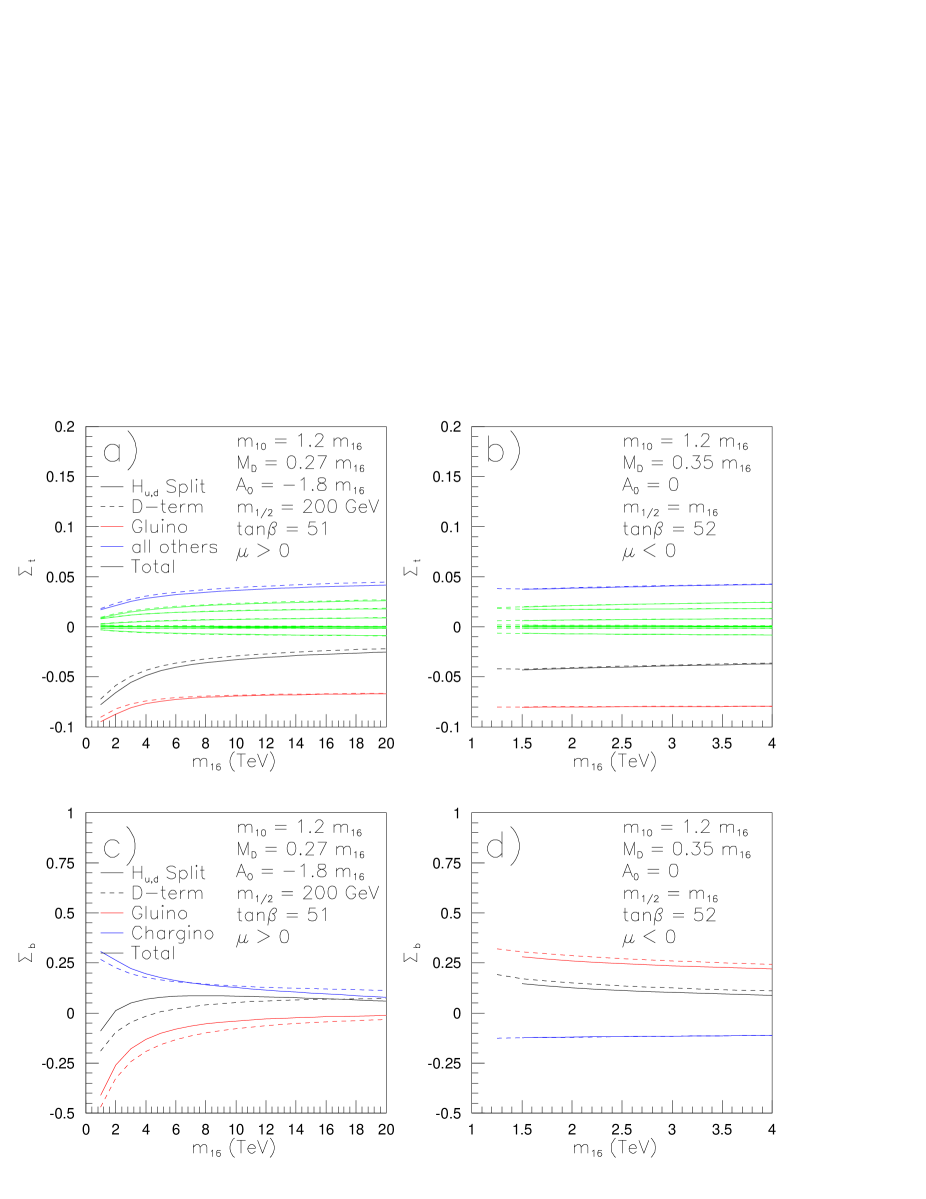
Figure 14: Various one loop contributions to the SUSY corrections to $m_{t}(m_{t})$ and $m_{b}(M_{Z})$ versus $m_{16}$, for the $DT$ and $HS$ models. The total corrections is shown by the dashed (solid) black line for the $DT$ ($HS$) model. various colored lines are as discussed in the text.

For $\mu>0$ in frame c), the best Yukawa unified solutions have $A_{t}<0$. As a consequence the gluino and chargino loops largely cancel. The difference between the $DT$ and $HS$ models is significant except for the largest values of $m_{16}$, and arises due to the differences in the values of squark masses in the two models. For the $\mu<0$ case in frame d), these contributions to $\Sigma_{b}$ flip sign relative to the $\mu>0$ case, as can be seen from Eq. (10). This correlation with the sign of the $\mu$–term makes it easier to obtain Yukawa unified solutions with $\mu<0$. There is also only a slight difference in this case between the $DT$ and $HS$ model, reflecting our results that for $\mu<0$, there is little preference between the two schemes as far as Yukawa unification is concerned.

In ISAJET, the scale $M_{GUT}$ is determined by the $Q$ value where $g_{1}$ and $g_{2}$ have a common value. A GUT scale splitting of $g_{1}$ and $g_{2}$ with $g_{3}$ is allowed since $g_{3}(M_{GUT})$ is determined by evolving the central value of $\alpha_{s}(M_{Z})$. In contrast, BDR allow an adjustable splitting between the GUT scale gauge couplings, and find that their best fit is obtained for a 3–4% deviation from perfect unification. Although this difference is amplified about four times at $Q=M_{Z}$ (and so could have been a potential cause of the difference), we see that, especially for pt. 1, in Table 1 that ISAJET results in a similar splitting between the gauge couplings. We conclude that the additional freedom provided by $\epsilon_{3}$ is unlikely to account for the difference between this analysis and that of BDR.

A possible criticism of our approach is that the Yukawa couplings are never truly unified, but only unified to within a specified tolerance. To get some idea of what would be a reasonable value for this tolerance, we show in Fig. 15 the Yukawa unification parameter $R$ versus the inputs $m_{b}^{\overline{DR}}(M_{Z})$ and $m_{t}$ for the $DT$ model (frames a) and b)) and for the $HS$ model (frames c) and d)) for several different sets of model parameters. The solid black curves in all four frames illustrates the variation of $R$ for the parameters listed in the upper frames. The dashed red and dot-dashed blue curves illustrate the variation of $R$ for pt. 1 of Table 1 and pt. 5 of Table 2, respectively. For these latter two points parameters are such that we are close to a local minimum of $R$. We vary $m_{b}^{\overline{DR}}(M_{Z})$ from 2.63 GeV to 3.03 GeV, which is its range quoted by the Particle Data Group, but recognize that recent calculations[44] suggest that the allowed range may be just about half as big. We vary the pole mass $m_{t}$ from 170 to 180 GeV. The curves are cut off if theoretical constraints that require REWSB or a neutralino LSP cannot be satisfied.

For the black curves, we see that as $m_{t}$ changes over its allowed range, $R$ varies by about 10%. We have checked that in this case, while $f_{b}(M_{GUT})$ is rather stable, $f_{t}(M_{GUT})$ changes from 0.56 for $m_{t}=175$ GeV to 0.62 for $m_{t}=180$ GeV, i.e. it is somewhat sensitive to the weak scale top Yukawa coupling, consistent with the finding of Ref.[45]; for $m_{t}$ smaller than about 175 GeV, the rise in the black curve in frame b) is due to a significant reduction in the corresponding bottom Yukawa coupling. The variation in $R$ due to variation in $m_{b}$ is twice as much, if we allow $m_{b}^{\overline{DR}}(M_{Z})$ to vary over the entire range suggested by the PDG compilation. For the parameters in pt. 5 of Table 2, the dot-dashed blue curve shows a minimum for our default choices of fermion mass. This should not be surprising because for this case, we have nearly perfect unification. The value of $R$ is rather sensitive to the bottom mass at the weak scale. Finally, for pt. 1 (which is also near a local minimum of $R$) of Table 1, we see that $R$ changes by less than 10% over the entire range of inputs for the top and bottom quark masses. Taking these cases to be representative, we see that while $R$ is somewhat sensitive to the weak scale fermion masses, the change in $R$ is $\lesssim 10\%$ as these are varied over their acceptable range, especially if we are already in the vicinity of a local minimum of $R$. We conclude that models with 5–10% Yukawa coupling unification may be regarded as viable.

4.2 Comparison of numerical results

Having compared and contrasted our procedure with the one used by BDR, we proceed to compare our numerical results with those in Ref. [18]. Since BDR focus on the positive $\mu$ case, our comparison is restricted to this. Both analyses agree in a number of important respects. The areas of agreement are:

• Yukawa unified solutions occur for $m_{16}\gg m_{1/2}$.

• The best Yukawa coupling unification occurs for boundary conditions close to the boundary conditions first dicussed for the RIMH scenario, viz. $A_{0}^{2}=2m_{10}^{2}=4m_{16}^{2}$ with $A_{0}=-2m_{16}$ fixing the sign of the $A_{0}$ term,

• For $\mu>0$, the $HS$ model leads to better unification of Yukawa couplings than the $DT$ model. The reason for this is discussed in the text.

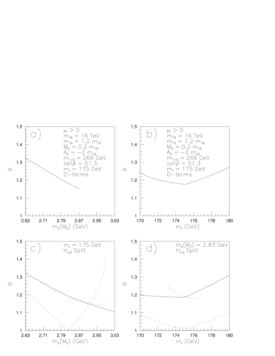
Figure 15: The Yukawa unification parameter $R$ versus $m_{t}$ (pole mass) and $m_{b}^{\overline{DR}}(M_{Z})$ for different sets of parameters of the $DT$ and $HS$ models. The solid black curves in all four frames correspond to the parameters listed in the frames a) and b) for the $DT$ model. The dashed red and dot-dashed blue curves in frames c) and d) for the $HS$ model correspond to pt. 1 of Table 1 and pt. 5 of Table 2, respectively. The curves are terminated if theoretical constraints are not satisfied.

There are, however, significant differences between our results and those in Ref.[18].

• Our analysis finds that $m_{16}\sim 8-15$ TeV is needed to achieve Yukawa coupling unification to a few per cent. BDR find acceptable models for $m_{16}$ as low as $\sim 1.5-2.5$ TeV, although their $\chi^{2}$ fits improve as $m_{16}$ increases. For these low $m_{1}6$ solutions, BDR find $\chi^{2}$ is typically larger than about 1; since we take our weak scale parameters to be their central experimental values, we do not expect to find such solutions.

• BDR find Yukawa unification for $m_{1/2}\sim 200-400$ GeV, with $\mu\lesssim m_{1/2}$. These models with a higgsino-like LSP ought to lead to a low value of neutralino relic density. We find $m_{1/2}\sim 0-200$ GeV, with $\mu>m_{1/2}$. In our results, low $|\mu|$ solutions can be generated, but the Yukawa unification never reaches the few per cent level.

• Our value of Yukawa couplings at $Q=M_{GUT}$ are typically around 0.5 to within about 10%. This is considerably lower than the BDR value of the unified Yukawa coupling which ranges from 0.63 – 0.8 for the explicit examples in Ref. [18]. For RIMH-like boundary conditions, third generation sfermion and Higgs boson mass squared parameters depend exponentially on the square of the Yukawa couplings so that this seemingly innocuous difference in Yukawa couplings could have considerable impact upon the spectrum.

The low $m_{16}$ solutions found by BDR lead to rather different expectations for sparticle masses compared to the results presented here. BDR find that $m_{A}\sim 100-200$ GeV, although values of $m_{A}$ up to 350 GeV are permitted.  They also find $m_{\tilde{t}_{1}}\sim 100-300$ GeV, $m_{\tilde{g}}\sim 500-1000$ GeV and $m_{\widetilde{W}_{1}}\sim 100-300$ GeV, where the latter particle has a significant higgsino component since $\mu$ is small. Our analysis finds $m_{A}\sim 1-2$ TeV, while $m_{\tilde{t}_{1}}\sim 500-2000$ GeV, $m_{\tilde{g}}\sim 300-500$ GeV and $m_{\widetilde{W}_{1}}\sim 100-250$ GeV, where the latter is gaugino-like. In addition, first and second generation matter scalars are at the multi-TeV level, which suppresses unwanted $FC$ and $CP$ violating processes, but which also makes it difficult to obtain a reasonable dark matter relic density.

There are also several differences in the numerical procedures of the two groups which could possibly account for the differences in the results.

• ISAJET uses the central values of the fermion masses and gauge couplings while BDR make a fit to the experimentally allowed windows. Tobe and Wells [45] have recently suggested that Yukawa couplings at $Q=M_{GUT}$ may be sensitive to their values at the weak scale; if this is the case then, as they suggest, the degree of Yukawa coupling unification may indeed be affected by the fact that BDR allow for an experimental window for weak scale parameters. This view is seemingly supported by the existence of a large $\tan\beta$ infrared fixed point for the top Yukawa coupling, as illustrated for instance in the second frame of Fig. 11 of Ref. [46]. However, we note that for values of $f_{t}(M_{GUT})$ that we find, we are far from this fixed point. Indeed, we have examined Yukawa coupling unification for the $HS$ model with $m_{t}=180$ GeV as well as $m_{t}=172$ GeV, and $\mu>0$. We find that the results are qualitatively similar to those in Fig. 3, except that $R_{min}$ is attained closer to 47–48 (51) for $m_{t}$ of 172 GeV (180 GeV), and the range of $M_{D}$ over which the minimum is attained is narrower for $m_{t}=180$ GeV. But the most important feature of these scans is that we can find solutions with better than 5% unification for essentially the same range of $m_{16}$ as in Fig. 3 for all three values of $m_{t}$ that we have examined. We also remark that a larger value of $f_{t}$ would take one closer to the fixed point solution, possibly resulting in the sensitivity suggested in Ref. [45]. We also note that for pt. 1 in Table 1, we found that increasing $m_{t}$ much beyond $\sim 176$ GeV lead to tachyonic $\widetilde{t}_{1}$, and that a change of the top Yukawa of this magnitude in $m_{t}$ resulted in a similar relative change in $f_{t}(M_{GUT})$. We do find other points where $f_{t}(M_{GUT})$ is senstive to the input value of $m_{t}$; however for these cases, the unification degree is not improved by changing $m_{t}$ (See Fig. 15, and accompanying discussion.).

• Motivated by the fact that the solutions in BDR (especially those in Table 2 that satisfy all phenomenological constraints), we performed a scan of the HS model for $\mu>0$ but taking $m_{b}^{\overline{DR}}(M_{Z})=3.03$ GeV. As in Fig. 3, we find that we obtain nearly perfect unification only if $m_{16}>8-10$ TeV. The biggest differences are that for $m_{b}=3.03$ GeV, $R\simeq 1$ may be obtained even if $m_{10}<m_{16}$, and the allowed range of $M_{D}$ is slightly reduced. Thus, it does not appear to us that variation of $m_{t}$ and $m_{b}$ about their central values will lead to Yukawa unified solutions with low $m_{16}$ as in BDR, unless we relax unification to the vicinity of $R\sim 1.2$.

• ISAJET minimizes the MSSM scalar potential at an optimal scale given by $\sqrt{m_{\widetilde{t}_{L}}m_{\widetilde{t}_{R}}}$ chosen to minimize residual scale dependent part of the one loop effective potential. BDR minimize the scalar potential at $M_{Z}$. The difference in the minimization scales may considerably affect the calculation of the $\mu$–term (recall that BDR find the best fits for very small values of $|\mu|$) and the sparticle mass spectrum. We recall that the dominant SUSY thresholds to $m_{b}$ are proportional to the $\mu$–term as can be seen in Eq. (10).

• ISAJET implements the one–loop logarithmic SUSY thresholds to gauge and Yukawa couplings through RGE decoupling while BDR implement all the susy thresholds, logarithmic and finite, using running parameters renormalized at the scale $M_{Z}$.

We have listed the probable sources of differences between the two approaches, but are unable to pinpoint any one of these as the main source of the difference from BDR results.

5 Summary and Concluding Remarks

We have implemented a number of improvements in the program ISAJET which are relevant for assessing the degree of third generation Yukawa coupling unification in supersymmetric models. Specifically, we examine $SO(10)$-inspired supersymmetric models with $D$-term splittings of scalar masses ($DT$ model), and with mass splittings applied only to the Higgs multiplets ($HS$ model). Using ISAJET v7.64, we have scanned a much larger region of parameter space than in our previous studies.

Models with $\mu>0$ appear to be favored by experimental measurements of $BF(b\rightarrow s\gamma)$ and the muon anomalous magnetic moment $a_{\mu}$. In these models, we find that Yukawa coupling unification is possible in the mSUGRA model at the 35% level; i.e. the relative difference between the largest and smallest of the third generation Yukawa couplings at $Q=M_{GUT}$ can be as low as 35%. In the $DT$ model, Yukawa unification may be possible at the 10% level, while in the $HS$ model, perfect Yukawa unification is possible. However, the high degree of unification requires SUSY scalars to be very heavy and gaugino masses to be much smaller. The parameter space of the $HS$ model in which Yukawa coupling unification occurs is characterized by

• $m_{10}\sim 1.2m_{16}$,

• $A_{0}\simeq-2m_{16}$,

• $\tan\beta\sim 48-50$,

• $m_{16}\sim 8-20$ TeV,

• $m_{1/2}\sim 0-400$ GeV.

Parameter ranges for good unification in the $DT$ model are qualitatively similar.

These boundary conditions for the soft SUSY breaking parameters are similar to those derived previously by Bagger et al. in the context of RIMH models, and was already noted by the BF and BDR analyses. The multi-TeV scalar masses are sufficient to yield a decoupling solution to the SUSY flavor and $CP$ problems. However, though some of the third generation scalars are considerably lighter, it appears that these models will require some fine-tuning to maintain the electroweak scale at the observed value. The Yukawa unified $HS$ models with $\mu>0$ yield values of $BF(b\rightarrow s\gamma)$ in accord with measurements, but they predict a value of muon anomalous magnetic moment $a_{\mu}$ close to the SM value, since SUSY contributions to $a_{\mu}$ in this case essentially decouple. More problematic is the value of neutralino relic density $\Omega_{\widetilde{Z}_{1}}h^{2}$, which is usually much greater than 1, and thus excluded. For $m_{16}$ values as low as $\sim 3$ TeV, it is possible to obtain reasonable values of the relic density, especially if $m_{\widetilde{Z}_{1}}\sim m_{h}/2$, so that resonance annihilation takes place. However, unification is then possible only at the level of 20%. Putting aside the issue of the relic density (for instance, if the LSP were unstable but long-lived), then for the $HS$ model with Yukawa unification, gluinos and charginos would be relatively light, and accessible to LHC experiments, and possibly even at the Tevatron or linear colliders. As discussed in detail in Sec. 4, our results agree in several respects with the recent work of BDR; however, there are also significant differences, such as the magnitude of the $\mu$ parameter for which Yukawa coupling unification is possible. While we have not been able to unequivocally track down the precise reasons for the differences, we have attempted to carefully compare and contrast the two approaches to facilitate this.

We have also re-examined Yukawa coupling unification for supersymmetric models with $\mu<0$. Both the $DT$ and the $HS$ models give qualitatively very similar results. Moreover, these results in this case are qualitatively similar to those derived in Refs. [14, 16]. Models with perfect Yukawa coupling unification can be found, but the region of parameter space is quite different from $\mu>0$ models. This is because of the sensitivity of the corrections to $m_{b}$ to the sign of $\mu$, that comes from cancellations that are necessary for Yukawa coupling unification if $\mu>0$. For negative values of $\mu$, the ranges of parameters for which good Yukawa unification is obtained are characterized by,

• $\tan\beta\sim 53-56$,

• $m_{16}\sim m_{1/2}$,

• $M_{D}\sim(0.2-0.4)m_{16}$.

However, these models tend to be disfavored by $BF(b\rightarrow s\gamma)$ and $a_{\mu}$. Nonetheless, they can be in accord with the relic density $\Omega_{\widetilde{Z}_{1}}h^{2}$, since a corridor of resonance annihilation through $s$-channel $A$ and $H$ poles runs through the region where a high degree of Yukawa coupling unification occurs. Generally, both $m_{16}$ and $m_{1/2}$ are large in these models, especially for model parameter choices in rough accord with $BF(b\rightarrow s\gamma)$ and $a_{\mu}$. Thus, usually the SUSY particles in this case are expected to be out of reach of Tevatron or LC experiments, and searches at the LHC may also prove very challenging.

SUSY GUT models based on the gauge group $SO(10)$ are highly motivated. In many of these models, it is expected that third generation Yukawa coupling unification should occur. We have shown that supersymmetric models consistent with Yukawa coupling unification exist for both $\mu>0$ and $\mu<0$. The requirement of Yukawa coupling unification greatly constrains the parameter space of the models. Typically, SUSY scalars are very heavy, and sometimes (especially for negative $\mu$) all sparticles may be heavy, perhaps even beyond the reach of the LHC. If weak scale supersymmetry is found at a future collider or non-accelerator experiments, it will be very interesting to see if the spectrum reflects qualities consistent with Yukawa coupling unification, perhaps pointing to $SO(10)$ as the proper gauge group for SUSY GUT models.

References

- [1] H. Georgi, in Proceedings of the American Institue of Physics, edited by C. Carlson (1974); H. Fritzsch and P. Minkowski, Ann. Phys. 93, 193 (1975); M. Gell-Mann, P. Ramond and R. Slansky, Rev. Mod. Phys. 50, 721 (1978). For recent reviews, see R. Mohapatra, hep-ph/9911272 (1999) and S. Raby, in Phys. Rev. D66, 010001 (2002).
- [2] M. Gell-Mann, P. Ramond and R. Slansky, in Supergravity, Proceedings of the Workshop, Stony Brook, NY 1979 (North-Holland, Amsterdam); T. Yanagida, KEK Report No. 79-18, 1979; R. Mohapatra and G. Senjanovic, Phys. Rev. Lett. 44, 912 (1980).
- [3] Y. Fukuda et al. Phys. Rev. Lett. 82, 2644 (1999) and 85, 3999 (2000).
- [4] For a review, see W. Buchmüller, [arXiv:hep-ph/0204288].
- [5] Some references include S. Dimopoulos, L. Hall and S. Raby, Phys. Rev. Lett. 68, 1984 (1992) and Phys. Rev. D46, 4793 (1992); G. Anderson, S. Raby, S. Dimopoulos, L. Hall and G. Starkman, Phys. Rev. D49, 3660 (1994); M. Carena, S. Dimopoulos, C. Wagner and S. Raby, Phys. Rev. D52, 4133 (1995); K. Babu and S. Barr, Phys. Rev. D56, 2614 (1997); K. Babu, J. Pati and F. Wilczek, Nucl. Phys. B566, 33 (2000); C. Albright and S. Barr, Phys. Rev. D58, 013002 (1998).
- [6] T. Blazek, M. Carena, S. Raby and C. Wagner, Phys. Rev. D56, 6919 (1997); T. Blazek and S. Raby, Phys. Lett. B392, 371 (1997); T. Blazek and S. Raby, Phys. Rev. D59, 095002 (1999); T. Blazek, S. Raby and K. Tobe, Phys. Rev. D 60, 113001 (1999) and Phys. Rev. D 62, 055001 (2000).
- [7] N. Sakai and T. Yanagida, Nucl. Phys. B197, 533 (1982); S. Weinberg, Phys. Rev. D26, 287 (1982).
- [8] S. Dimopoulos and F. Wilczek, Print-81-0600 (SANTA BARBARA); B. Grinstein, Nucl. Phys. B206, 387 (1982); R. Cahn, I. Hinchliffe, L. Hall, Phys. Lett. B109, 126 (1982); A. Masiero et al. Phys. Lett. B115, 380 (1982); I. Antoniadis et al. Phys. Lett. B194, 231 (1987); R. Barbieri, G. Dvali and S. Moretti, Phys. Lett. B312, 137 (1993); K. S. Babu and S. M. Barr, Phys. Rev. D 48, 5354 (1993); R. Barbieri et al. Nucl. Phys. B432, 49 (1994) Z. Berezhiani, Phys. Lett. B355, 481 (1995).
- [9] Y. Kawamura, Prog. Theor. Phys. 105, 999 (2001); G. Altarelli and F. Feruglio, Phys. Lett. B511, 257 (2001); L. Hall and Y. Nomura, Phys. Rev. D64, 055003 (2001); A. Hebecker and J. March-Russell, Nucl. Phys. B613, 3 (2001). A. Kobakhidze, Phys. Lett. B514, 131 (2001).
- [10] L. Hall and Y. Nomura, Phys. Rev. D65, 035008 (2002); T. Asaka, W. Buchmüller and L. Covi, Phys. Lett. B523, 199 (2001); A. Hebecker and J. March-Russell, Nucl. Phys. B625, 128 (2002); R. Dermisek and A. Mafi, Phys. Rev. D65, 055002 (2002); H. Baer, C. Balazs, A. Belyaev, R. Dermisek, A. Mafi and A. Mustafayev, J. High Energy Phys. 0205 (061) 2002; S. M. Barr and I. Dorsner, Phys. Rev. D66, 065013 (2002); H. D. Kim and S. Raby, JHEP 0301, 056 (2003).
- [11] See e.g. B. Ananthnarayan, G. Lazarides and Q. Shafi, Phys. Rev. D44, 1613 (1991) and Phys. Lett. B300, 245 (1993); G. Anderson et al. Phys. Rev. D47, 3702 (1993) and Phys. Rev. D49, 3660 (1994); V. Barger, M. Berger and P. Ohmann, Phys. Rev. D49, 4908 (1994); M. Carena, M. Olechowski, S. Pokorski and C. Wagner, Nucl. Phys. B426, 269 (1994); B. Ananthanarayan, Q. Shafi and X. Wang, Phys. Rev. D50, 5980 (1994); R. Rattazzi and U. Sarid, Phys. Rev. D53, 1553 (1996); see also T. Blazek, S. Raby and K. Tobe, Ref. [5].
- [12] H. Baer, J. Ferrandis and X. Tata, [arXiv:hep-ph/0211418]
- [13] R. Hempfling, Phys. Rev. D49, 6168 (1994); L. J. Hall, R. Rattazzi and U. Sarid, Phys. Rev. D50, 7048 (1994); M. Carena et al. Nucl. Phys. B426, 269 (1994).
- [14] H. Baer, M. A. Diaz, J. Ferrandis and X. Tata, Phys. Rev. D 61, 111701 (2000).
- [15] M. Drees, Phys. Lett. B181, 279 (1986); J.S. Hagelin and S. Kelley, Nucl. Phys. B342, 95 (1990); A.E. Faraggi, et al., Phys. Rev. D45, 3272 (1992); Y. Kawamura and M. Tanaka, Prog. Theor. Phys. 91, 949 (1994); Y. Kawamura, et al., Phys. Lett. B324, 52 (1994); Phys. Rev. D51, 1337 (1995); N. Polonsky and A. Pomarol, Phys. Rev. D51, 6532 (1994); H.-C. Cheng and L.J. Hall, Phys. Rev. D51, 5289 (1995); C. Kolda and S.P. Martin, Phys. Rev. D53, 3871 (1996).
- [16] H. Baer, M. Brhlik, M. A. Diaz, J. Ferrandis, P. Mercadante, P. Quintana and X. Tata, Phys. Rev. D 63, 015007 (2001) [arXiv:hep-ph/0005027].
- [17] H. N. Brown et al., (E821 Collaboration), Phys. Rev. Lett. 86 (2001) 2227 and Phys. Rev. Lett. 89 (101804) 2002.
- [18] T. Blazek, R. Dermisek and S. Raby, Phys. Rev. Lett. 88, 111804 (2002) and Phys. Rev. D65, 115004 (2002).
- [19] H. Baer and J. Ferrandis, Phys. Rev. Lett. 87, 211803 (2001).
- [20] U. Chattopadhyay and P. Nath, Phys. Rev. D65, 075009 (2002); U. Chattopadhyay, A. Corsetti and P. Nath, Phys. Rev. D66, 035003 (2002).
- [21] M. E. Gomez, G. Lazarides and C. Pallis, Phys. Rev. D61, 123512 (2000), Phys. Lett. B487, 313 (2000), Nucl. Phys. B 638, 165 (2002) and [arXiv:hep-ph/0301064].
- [22] J. Feng, C. Kolda and N. Polonsky, Nucl. Phys. B546, 3 (1999); J.Bagger, J. Feng and N. Polonsky, Nucl. Phys. B563, 3 (1999); J. Bagger, J. Feng, N. Polonsky and R. Zhang, Phys. Lett. B473, 264 (2000).
- [23] H. Baer, P. Mercadante and X. Tata, Phys. Lett. B475, 289 (2000); H. Baer, C. Balázs, M. Brhlik, P. Mercadante, X. Tata and Y. Wang, Phys. Rev. D64, 015002 (2001).
- [24] D. Pierce, J. Bagger, K. Matchev and R. Zhang, Nucl. Phys. B491, 3 (1997).
- [25] ISAJET, by F. Paige, S. Protopopescu, H. Baer and X. Tata, hep-ph/0001086 (2000).
- [26] Suspect, by A. Djouadi, J. Kneur and G. Moultaka, hep-ph/0211331 (2002).
- [27] B. Allanach, Comput. Phys. Commun. 143, 305 (2002).
- [28] W. Porod, [arXiv:hep-ph/0301101].
- [29] B. Allanach, S. Kraml and W. Porod, [arXiv:hep-ph/0302102].
- [30] H. Baer, J. Ferrandis, K. Melnikov and X. Tata, Phys. Rev. D 66, 074007 (2002).
- [31] A. Chamseddine, R. Arnowitt and P. Nath, Phys. Rev. Lett. 49 (1982) 970; R. Barbieri, S. Ferrara and C. Savoy, Phys. Lett. B 119 (1982) 343; L. J. Hall, J. Lykken and S. Weinberg, Phys. Rev. D 27 (1983) 2359.
- [32] I. Jack and D. R. T. Jones, Phys. Lett. B333, 372 (1994); S. Martin and M. Vaughn, Phys. Rev. D50, 2282 (1994); see also, Y. Yamada, Phys. Rev. D50, 3537 (1994).
- [33] H. Baer, X. Tata and J. Woodside, Phys. Rev. D41, 906 (1990).
- [34] H. Baer, M. Drees, F. Paige, P. Quintana and X. Tata, Phys. Rev. D61, 095007 (2000); V. Barger and C. Kao, Phys. Rev. D60, 115015 (1999); K. Matchev and D. Pierce, Phys. Lett. B467, 225 (1999).
- [35] S. Abel et al. (SUGRA Working Group Collaboration), hep-ph/0003154 (2000).
- [36] H. Baer, C. Balazs, J. Ferrandis and X. Tata, Phys. Rev. D64, 035004 (2001).
- [37] H. Baer and M. Brhlik, Phys. Rev. D55, 3201 (1997); H. Baer, M. Brhlik, D. Castaño and X. Tata, Phys. Rev. D58, 015007 (1998).
- [38] J. K. Mizukoshi, X. Tata and Y. Wang, Phys. Rev. D 66, 115003 (2002).
- [39] H. Baer and M. Brhlik, Phys. Rev. D53, 597 (1996) and Phys. Rev. D57, 567 (1998); H. Baer, C. Balazs and A. Belyaev, JHEP 0203, 042 (2002) and hep-ph/0211213 (2002); H. Baer, C. Balazs, A. Belyaev, J. K. Mizukoshi, X. Tata and Y. Wang, JHEP 0207, 050 (2002) and [arXiv:hep-ph/0210441].
- [40] See T. Blazek and S. Raby, Ref. [6] and also T. Blazek and S. F. King, Phys. Lett. B 518, 109 (2001).
- [41] J. Feng, K. Matchev and T. Moroi, Phys. Rev. Lett. 84, 2322 (2000) and Phys. Rev. D61, 075005 (2000); J. Feng, K. Matchev and F. Wilczek, Phys. Lett. B482, 388 (2000) and Phys. Rev. D63, 045024 (2001).
- [42] J. Ellis, T. Falk, G. Ganis, K. Olive and M. Srednicki, Phys. Lett. B510, 236 (2001);
- [43] M. Drees and M. Nojiri, Phys. Rev. D47, 376 (1993); H. Baer and M. Brhlik, Ref. [39]; J. Ellis et al. Ref. [42].
- [44] K. Melnikov and A. Yelkhovsky, Phys. Rev. D59, 114009 (1999); A.H. Hoang, Phys. Rev. D61, 034005 (2000); M. Beneke and A. Signer, Phys. Lett. B471, 233 (1999); A. A. Penin and A. A. Pivovarov, Nucl. Phys. B549, 217 (1999); V. Giménez, L. Giusti, G. Martinelli and F. Rapuano, JHEP, 03, 018 (2000).
- [45] K. Tobe and J. D. Wells, [arXiv:hep-ph/0301015].
- [46] B. Schrempp and M. Wimmer, Prog. in Part. and Nucl. Phys. 37, 1 (1996).