Affleck-Dine mechanism with negative thermal logarithmic potential

Abstract

We investigate whether the Affleck-Dine (AD) mechanism works when the contribution of the two-loop thermal correction to the potential is negative in the gauge-mediated supersymmetry breaking models. The AD field is trapped far away from the origin by the negative thermal correction for a long time until the temperature of the universe becomes low enough. The most striking feature is that the Hubble parameter becomes much smaller than the mass scale of the radial component of the AD field, during the trap. Then, the amplitude of the AD field decreases so slowly that the baryon number is not fixed even after the onset of radial oscillation. The resultant baryon asymmetry crucially depends on whether the Hubble parameter, $H$, is larger than the mass scale of the phase component of the AD field, $M_{\theta}$, at the beginning of oscillation. If $H<M_{\theta}$ holds, the formation of Q balls plays an essential role to determine the baryon number, which is found to be washed out due to the nonlinear dynamics of Q-ball formation. On the other hand, if $H>M_{\theta}$ holds, it is found that the dynamics of Q-ball formation does not affect the baryon asymmetry, and that it is possible to generate the right amount of the baryon asymmetry.

I Introduction

Baryogenesis is one of the main issues in the theories of the early universe. There have been proposed various mechanisms, among which Affleck-Dine (AD) mechanism AD is a promising candidate in theories with supersymmetry (SUSY). One of the features which distinguish supersymmetric theories from ordinary ones is the existence of flat directions, of which the AD mechanism makes use. In fact, there are many flat directions in the minimal supersymmetric standard model (MSSM), along which there are no classical potentials. Such a flat direction is described by a complex scalar field $\Phi$, called AD field. It is crucial to determine the dynamics of the AD field to estimate the resultant baryon asymmetry. However, it has been found that the AD baryogenesis is complicated by the two causes. One is the thermal effect thermal ; thermal2 ; anisimov , and the other is the existence of Q balls Kusenko ; Enqvist ; Kasuya1 .

As for the thermal effects, we must take account of those which appear at both one-loop and two-loop orders. The former contribution to the effective potential of the AD field is the thermal mass term which might cause the early oscillation of the AD field. The latter effect, on which we would like to focus in this paper, induces the logarithmic potential (which we call thermal log potential hereafter) and hence totally changes the dynamics if its coefficient is negative. In that case, the AD field might be trapped far away from the origin for a long time until the temperature of the universe becomes low enough. In particular, such a trap is likely to occur in the gauge-mediated supersymmetry breaking (GMSB) models gmsb where the potential for the AD field becomes flat at large amplitude. Therefore, we assume the GMSB models in this paper. Due to the enduring trap by the negative thermal log potential, the dynamics of the system is so involved that little has been known about whether the AD baryogenesis really works. Although the sign of the thermal contribution to the potential at two-loop order depends on the choice of flat directions, it is expected to be negative for many flat directions. Hence it is important to consider the case when the negative thermal log potential is effective.

The other element which we need to incorporate is the existence of Q balls Kusenko ; Enqvist ; Kasuya1 . After the AD field starts to oscillate, it experiences spatial instabilities and deforms into nontopological solitons, Q balls. Especially, the Q-ball formation is inevitable for a flat potential as in the GMSB models  Kasuya1 ; Kasuya2 ; Kasuya3 . Once Q balls are formed, they absorb almost all the baryon numbers Kasuya1 ; Kasuya3 . In the usual picture, the Q-ball formation takes place after the baryon number is fixed. However, as shown later, the Q-ball formation plays an essential role to fix the baryon number if the AD field is trapped by the negative thermal log potential.

In this paper, therefore, we consider the AD baryogenesis with the negative thermal log potential in the GMSB models, taking into account the Q-ball formation. Since the negative thermal log potential retards the oscillation of the AD field considerably, the dynamics is quite different from that for the ordinary AD baryogenesis, and we need to examine the scenario carefully. It is found that the existence of the Hubble-induced A-term spoils the baryogenesis through the Q-ball formation, while it is possible to explain the baryon asymmetry of the present universe in the absence of the Hubble-induced A-term.

II Affleck-Dine Mechanism and Q-ball formation

In this section we briefly review the Affleck-Dine mechanism and properties of the Q balls. In the MSSM, there exist flat directions, along which there are no classical potentials in the supersymmetric limit. Since flat directions consist of squarks and/or sleptons, they carry baryon and/or lepton numbers, and can be identified as the AD field. These flat directions are lifted by both the supersymmetry breaking effects and the nonrenormalizable operators with some cutoff scale. In the gauge-mediated SUSY breaking model, the potential of a flat direction is parabolic at the origin, and almost flat beyond the messenger scale Kusenko ; Kasuya3 ; Gouvea ,

$$V_{gauge}\sim\left\{\begin{array}[]{ll}m_{\phi}^{2}|\Phi|^{2}&\quad(|\Phi|\ll M_{S}),\\ \displaystyle{M_{F}^{4}\left(\log\frac{|\Phi|^{2}}{M_{S}^{2}}\right)^{2}}&\quad(|\Phi|\gg M_{S}),\\ \end{array}\right.$$ (1)

where $m_{\phi}$ is a soft breaking mass $\sim$ O(1 TeV), $M_{F}$ the SUSY breaking scale, and $M_{S}$ the messenger mass scale. Since the gravity always exists, flat directions are also lifted by the gravity-mediated SUSY breaking effects EnqvistMcDonald98 ,

$$V_{grav}\simeq m_{3/2}^{2}\left[1+K\log\left(\frac{|\Phi|^{2}}{M_{G}^{2}}\right)\right]|\Phi|^{2},$$ (2)

where $K$ is the numerical coefficient of the one-loop corrections and $M_{G}$ is the gravitational scale ($\simeq 2.4\times 10^{18}$ GeV). This term can be dominant only at high energy scales because of small gravitino mass $\lesssim O(1\mbox{ GeV})$.

The nonrenormalizable operators, in addition, lift flat directions. Assuming that there exist all the nonrenormalizable operators consistent with both the gauge symmetries of the standard model and the R-parity in the superpotential, most of flat directions are lifted by the following operator:

$$W=\frac{1}{nM^{n-3}}\Phi^{n}\,,$$ (3)

where $M$ is the cutoff scale. Not only does it lift the flat potential as

$$V_{NR}=\frac{|\Phi|^{2n-2}}{M^{2n-6}}\,,$$ (4)

but it supplies the baryon number violating A-term as

$$V_{A}=a_{m}\frac{m_{3/2}}{nM^{n-3}}\Phi^{n}+{\rm H.c.}\,,$$ (5)

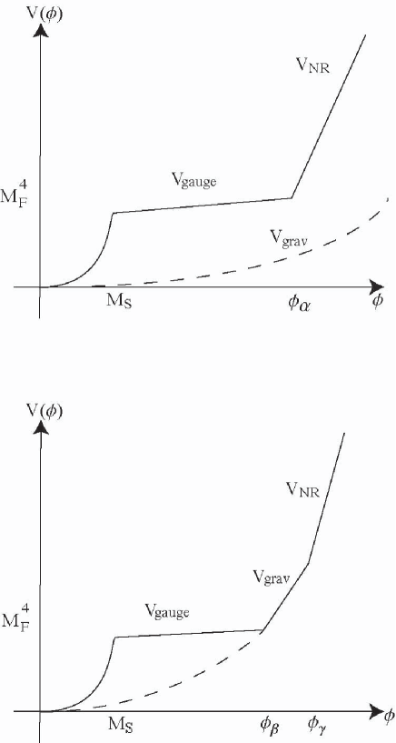
Figure 1: Schema for the zero-temperature potential $V_{gauge}+V_{gra}+V_{NR}$. If $m_{3/2}<M_{F}^{\frac{2n-4}{n-1}}M^{-\frac{n-3}{n-1}}$ is satisfied, the potential takes the form shown in the upper figure. The $V_{gauge}$-dominant region connects to the non-renormalizable term dominant region at $\phi_{\alpha}\simeq\left(M_{F}^{2}M^{n-3}\right)^{\frac{1}{n-1}}$. On the other hand, if $m_{3/2}>M_{F}^{\frac{2n-4}{n-1}}M^{-\frac{n-3}{n-1}}$ is satisfied, the potential takes the form shown in the lower figure. The $V_{gauge}$-dominant region connects to the $V_{grav}$-dominant region at $\phi_{\beta}\simeq\frac{M_{F}^{2}}{m_{3/2}}$, and then it connects to the non-renormalizable term dominant region at $\phi_{\gamma}\simeq(m_{3/2}M^{n-3})^{\frac{1}{n-2}}$.

where $a_{m}$ is a complex constant of order unity, and we assume the vanishing cosmological constant. The schema of the zero-temperature potential $V_{gauge}+V_{grav}+V_{NR}$ is shown in Fig. 1.

For the AD baryogenesis to work successfully, it is necessary that the AD field has a large expectation value during the inflationary epoch . To this end we require the existence of the four-point coupling of the AD field to the inflaton $I$ in the Kähler potential, which leads to the negative Hubble-induced mass term:

$$V_{H}=-c_{H}H^{2}|\Phi|^{2}\,,$$ (6)

where $c_{H}$ is a positive constant of order unity. Also there might be a Hubble-induced A-term, which comes from the three-point coupling of the AD field to the inflaton in the Kähler potential. We write it as

$$V_{AH}=a_{H}\frac{H}{nM^{n-3}}\Phi^{n}+{\rm H.c.}\,,$$ (7)

where $a_{H}$ is a complex constant of order unity. Though the presence of this term usually does not change the resultant baryon asymmetry, it does change the dynamics of the AD field when the negative thermal log potential traps the AD field, as shown later. Since the Hubble-induced A-term is not necessarily present, we will consider both cases with and without this term.

Let us consider the thermal effects on the effective potential for the AD field. During the oscillation of the inflaton, there is dilute plasma with temperature $T\sim(T_{RH}^{2}HM_{G})^{1/4}$, where $T_{RH}$ is the reheating temperature. If the AD field directly couples with fields $\psi_{k}$ in the thermal bath, it acquires a thermal mass term in the effective potential at one-loop order:

$$V_{T}^{(1)} \simeq \sum_{f_{k}|\Phi|<T}c_{k}f_{k}^{2}T^{2}|\Phi|^{2},$$ (8)

$$= f_{(1)}^{2}T^{2}|\Phi|^{2}{\rm~{}~{}~{}~{}for~{}}|\Phi|<f_{(1)}^{-1}T,$$

where $c_{k}$ is a real positive constant of order unity, and $f_{k}$ is a Yukawa, or gauge coupling constant between the AD field and $\psi_{k}$ thermal2 ; afhy . For simplicity, we omit the subscript $k$ hereafter with the understanding that $f_{(1)}$ denotes either Yukawa or gauge coupling constant. Note that this effect is exponentially suppressed by the Boltzmann factor when the effective mass of the thermal particle, $f_{(1)}|\Phi|$, is larger than the temperature. In addition to this term, there is another thermal effect on the potential, which appears at two-loop order, as pointed out in Ref. anisimov . This comes from the fact that the running of the coupling constant is modified by integrating out heavy particles which directly couples with the AD field. This contribution is given by afhy2

$$V_{T}^{(2)}\sim a_{T}f_{(2)}^{4}T^{4}\log\frac{|\Phi|^{2}}{T^{2}},$$ (9)

where $a_{T}$ is an O(1) constant, and $f_{(2)}^{4}=g^{4},y^{4},y^{2}g^{2}$ ($g$ and $y$ are the gauge and Yukawa coupling constants). The sign of $a_{T}$ depends on the flat directions, and it is expected to be negative for many flat directions, for instance, $\overline{u}\overline{d}\overline{d}$ direction, though it is complicated to determine the precise value of $a_{T}$. Without specifying flat directions, we would like to focus on the case with the negative $a_{T}$ in the following discussion. (The AD baryogenesis for the positive $a_{T}$ was considered in Ref. Kasuya3 .)

When the AD field starts coherent rotation in the potential, the baryon number is generated and fixed immediately in the ordinary AD mechanism, since the A-terms becomes ineffective soon after the oscillation of the AD field. Then the baryon number density is estimated as

$$n_{B}(t_{osc})\simeq\varepsilon\omega\phi_{osc}^{2},$$ (10)

where $\varepsilon(\lesssim 1)$ is the ellipticity parameter, which represents the strongness of the A-term, and $\omega$ and $\phi_{osc}$ are the angular velocity and the amplitude of the AD field respectively, at the beginning of the oscillation (rotation) in its effective potential. However, this is not the case when the AD field is trapped by the negative thermal log potential given by Eq. (9), which will be discussed in the next section. In fact, the baryon number is not fixed even after the AD field starts coherent oscillation, if the Hubble parameter is much smaller than the mass scale of the radial direction. It should be emphasized that Eq. (10) is valid as long as the baryon number is fixed soon after the oscillation commenced.

Lastly, we comment on the Q balls. In the course of the coherent oscillation, the AD field experiences spatial instabilities, and deforms into nontopological solitons, Q balls  Kusenko ; Enqvist ; Kasuya1 . When the effective potential is dominated by the zero-temperature term $V_{gauge}$, the gauge-mediation type Q balls are formed, whose properties are as follows Dvali :

$$M_{Q}\sim M_{F}Q^{3/4},\qquad R_{Q}\sim M_{F}^{-1}Q^{1/4},$$ (11)

where $M_{Q}$ and $R_{Q}$ are the mass and the size of the Q ball, respectively. If the mass per unit charge, $M_{F}Q^{-1/4}$, is smaller than the proton mass $\sim$ 1GeV, the Q ball is stable against the decays into nucleons, from which it follows that Q balls with very large $Q$ can be stable. From numerical calculations Kasuya1 ; Kasuya3 , it is known that Q balls absorb almost all the baryon charges which the AD field obtains, and the typical charge is estimated as Kasuya3

$$Q\simeq\beta\left(\frac{\phi_{osc}}{M_{F}}\right)^{4},$$ (12)

where $\beta\approx 6\times 10^{-4}$. Consequently, the present baryon asymmetry should be explained by the charges which come out of the Q balls through the evaporation and decay of Q balls.

In the case of the unstable Q balls, they decay into nucleons. The decay rate is given by Coleman

$$\left|\frac{dQ}{dt}\right|\lesssim\frac{\omega^{3}A}{192\pi^{2}},$$ (13)

where $A$ is a surface area of the Q ball.

In the case of the stable Q balls, the evaporation is the only way to extract the baryon charges from Q balls. The total evaporated charge from the Q ball is estimated as Kasuya3 ; Laine ; Banerjee ,

$$\Delta Q\sim 10^{15}\left(\frac{m_{\phi}}{\mbox{TeV}}\right)^{-2/3}\left(\frac{M_{F}}{10^{6}\mbox{GeV}}\right)^{-1/3}Q^{1/12}.$$ (14)

Hence the baryon number density is suppressed by the factor $\Delta Q/Q$, in comparison with the case of unstable Q-ball production.

III Dynamics of Affleck-Dine field

In this section, we present a detailed discussion on the dynamics of the AD field. First we derive the condition that the AD field is trapped by the negative thermal log potential. In the following argument we set $|a_{m}|=c_{H}=|a_{H}|=c_{k}=-a_{T}=1$ for simplicity. During inflation the Hubble parameter is roughly constant, and the initial amplitude of AD field is set far away from the origin due to the negative Hubble-induced mass term Eq. (6). The position of the global minimum is

$$\phi\simeq(HM^{n-3})^{1/(n-2)}\,,$$ (15)

where $\phi\equiv\sqrt{2}|\Phi|$. After inflation ends, the Hubble parameter decreases, and so does the minimum of the potential. Since the AD field tracks the instantaneous minimum, Eq.(15) still holds after inflation. The AD field is trapped by the negative thermal log potential when $|V_{T}^{(2)}|>|V_{H}|$ is satisfied. Here we assumed that the trap due to the negative thermal log potential occurs while the AD field tracks the instantaneous minimum given as Eq.(15). The temperature $T_{c}$ and the amplitude $\phi_{c}$ at the beginning of the trap are

$$T_{c} = \left\{\begin{array}[]{ll}\displaystyle{f_{(2)}^{\frac{n-2}{n}}T_{RH}^{\frac{n-1}{n}}M_{G}^{\frac{n-1}{2n}}M^{-\frac{(n-3)}{2n}}}&{\rm for~{}~{}}\displaystyle{T_{RH}<T_{*},}\\ &\\ \displaystyle{T_{*}}&{\rm for~{}~{}}\displaystyle{T_{RH}>T_{*},}\end{array}\right.$$ (17)

$$\phi_{c} = \left(f_{(2)}^{2}T_{c}^{2}M^{n-3}\right)^{\frac{1}{n-1}},$$ (18)

where we defined

$$T_{*}\equiv f_{(2)}^{n-2}M_{G}^{\frac{n-1}{2}}M^{-\frac{n-3}{2}}.$$ (19)

It should be noted that $T_{RH}>T_{*}$ requires a very high reheating temperature which might be constrained by the gravitino problem Gouvea . However, if the Q balls dominate the universe, they must decay and reheat the universe with the decay temperature, $T_{d}\lesssim O(1{\rm GeV})$. Thus the gravitino problem is alleviated due to the entropy production of the decay of Q balls in this case, and such a high reheating temperature might be possible. If it were not for the gravitino problem, the reheating temperature could be as large as $T_{inf}\equiv 10^{16}$ GeV. We take this value, because the COBE data implies that $V_{inf}^{1/4}/\epsilon_{sr}^{1/4}\simeq 6.7\times 10^{16}$ GeV LyRi , where $\epsilon_{sr}<1$ is the slow-roll parameter, and the instantaneous reheating is assumed for conservative discussion.

Next we consider when the trap due to the negative thermal log potential ends. The AD field starts an oscillation when $|V_{T}^{(2)}|<V_{gauge}$ is first satisfied, hence the temperature $T_{osc}$ and the amplitude $\phi_{osc}$ at that moment are

$$T_{osc} = f_{(2)}^{-1}M_{F}\,,$$

$$\phi_{osc} = {\rm min}\left[\phi_{\alpha},~{}\phi_{\beta}\right],$$ (20)

where $\phi_{\alpha}\equiv\left(M_{F}^{2}M^{n-3}\right)^{\frac{1}{n-1}}$ and $\phi_{\beta}\equiv M_{F}^{2}/m_{3/2}$. Note that the amplitude of the AD field, $\phi_{osc}$, at the beginning of oscillation is different from that in the usual scenario. In the ordinary AD mechanism, the AD field starts oscillating at $\phi_{\alpha}$ or $\phi_{\gamma}\equiv(m_{3/2}M^{n-3})^{\frac{1}{n-2}}$ depending on the form of the potential shown in Fig. 1, if one does not take account of the thermal effects. Such modification is due to the different dependence of $V_{H}$ and $V_{T}^{(2)}$ on $\Phi$.

From the above discussion we can derive the condition that the AD field is trapped by the negative thermal log potential. It requires the following inequalities to be satisfied.

$$\phi_{c} > {\rm Max}\left[\phi_{\alpha},\phi_{\gamma}\right],$$ (21)

$$f_{(1)}\phi_{c} > T_{c},$$ (22)

$$\phi_{osc} > M_{S}.$$ (23)

Then we arrive at the following conditions.

$$10^{-5}{\rm~{}GeV}\lesssim m_{3/2} \lesssim m_{3/2}^{(u)},$$

$$10{\rm~{}TeV}\lesssim M_{F} \lesssim M_{F}^{(u)},$$

$$T_{RH}^{(l)}\lesssim T_{RH} \lesssim T_{RH}^{(u)}\,,$$ (24)

where $m_{3/2}^{(u)}$, $M_{F}^{(u)}$, $T_{RH}^{(l)}$ and $T_{RH}^{(u)}$ are given as

$$m_{3/2}^{(u)} \equiv \left\{\begin{array}[]{ll}\displaystyle{1{\rm~{}GeV}}&\displaystyle{{\rm for~{}~{}}T_{RH}<T_{*}},\\ &\\ \displaystyle{{\rm Min}\left[1{\rm~{}GeV},~{}f_{(2)}^{2n-4}M_{G}^{n-2}M^{-(n-3)}\right]}&\displaystyle{{\rm for~{}~{}}T_{RH}>T_{*},~{}M>f_{(1)}^{\frac{-2}{n-3}}f_{(2)}^{\frac{2(n-4)}{n-3}}M_{G}},\end{array}\right.$$ (28)

$$M_{F}^{(u)} \equiv \left\{\begin{array}[]{ll}\displaystyle{{\rm Min}\left[\sqrt{m_{3/2}M_{G}},~{}\left(m_{\phi}^{n-1}M^{n-3}\right)^{\frac{1}{2n-4}}\right]}&\displaystyle{{\rm for~{}~{}}T_{RH}<T_{*}},\\ &\\ \displaystyle{{\rm Min}\left[\sqrt{m_{3/2}M_{G}},~{}\left(m_{\phi}^{n-1}M^{n-3}\right)^{\frac{1}{2n-4}},~{}f_{(2)}^{n-1}M_{G}^{\frac{n-1}{2}}M^{-\frac{(n-3)}{2}}\right]}&\displaystyle{{\rm for~{}~{}}T_{RH}>T_{*},~{}M>f_{(1)}^{\frac{-2}{n-3}}f_{(2)}^{\frac{2(n-4)}{n-3}}M_{G}},\end{array}\right.$$ (32)

$$T_{RH}^{(l)} \equiv f_{(2)}^{-2}M_{G}^{-\frac{1}{2}}\times{\rm Max}\left[\left(m_{3/2}^{n}M^{2(n-3)}\right)^{\frac{1}{2(n-2)}},~{}\left(M_{F}^{2n}M^{n-3}\right)^{\frac{1}{2(n-1)}}\right],$$ (33)

$$T_{RH}^{(u)} \equiv \left\{\begin{array}[]{ll}T_{inf}&{\rm for~{}~{}}\displaystyle{M>f_{(1)}^{\frac{-2}{n-3}}f_{(2)}^{\frac{2(n-4)}{n-3}}M_{G}}\\ &\\ {\rm Min}\displaystyle{\left[f_{(1)}^{\frac{n}{n-3}}f_{(2)}^{\frac{-n+6}{n-3}}M_{G}^{-\frac{1}{2}}M^{\frac{3}{2}},~{}~{}T_{inf}\right]}&{\rm for~{}~{}}\displaystyle{M<f_{(1)}^{\frac{-2}{n-3}}f_{(2)}^{\frac{2(n-4)}{n-3}}M_{G}},\\ \end{array}\right.$$ (37)

where we do not take account of the gravitino problem, and the bounds for $M_{F}$ and $m_{3/2}$ include the constraints due to the scheme of the GMSB. Notice that $T_{RH}^{(l)}$ comes from $\phi_{c}>{\rm Max}[\phi_{\alpha},\phi_{\gamma}]$ and $T_{RH}^{(u)}$ is obtained from the condition $f_{(1)}\phi_{c}>T_{c}$. Also, we must impose the following condition in order to take the gravitino problem Gouvea into consideration.

$$T_{RH}<\gamma\times\left\{\begin{array}[]{ll}100{\rm GeV}\sim 1{\rm TeV}&{\rm for~{}~{}}\displaystyle{2h^{2}{\rm keV}\lesssim m_{3/2}\lesssim 100{\rm keV}}\\ &\\ \displaystyle{10{\rm TeV}\times h^{2}\left(\frac{m_{3/2}}{100{\rm keV}}\right)\left(\frac{m_{G3}}{1{\rm TeV}}\right)^{-2}}&{\rm for~{}~{}}\displaystyle{m_{3/2}>100{\rm keV}},\end{array}\right.$$

where $h$ is the present Hubble parameter in units of 100km/sec/Mpc, $m_{G3}$ is the gaugino mass for $SU(3)_{C}$, and $\gamma$ reflects the entropy dilution due to the decay of Q-balls. If Q balls are subdominant component of the universe throughout, we have $\gamma=1$. On the other hand, if Q balls dominate the universe, it is given as

$$\gamma=\left\{\begin{array}[]{ll}\displaystyle{\frac{T_{RH}}{T_{d}}}&{\rm for~{}~{}}\displaystyle{T_{eq}>T_{RH}},\\ &\\ \displaystyle{\frac{T_{eq}}{T_{d}}}&{\rm for~{}~{}}\displaystyle{T_{eq}<T_{RH}},\end{array}\right.$$

where $T_{eq}$ is the temperature at which the energy of Q balls becomes comparable to the total energy of the universe, and $T_{d}$ is the decay temperature of Q balls given as

$$T_{d}=\left(\frac{\pi^{2}g_{*}}{90}\right)^{-\frac{1}{4}}\sqrt{\frac{M_{F}M_{G}}{48\pi Q^{\frac{5}{4}}}}\,,$$ (38)

where $g_{*}$ counts the effective degrees of freedom of the radiation.

So far we have outlined the dynamics of the amplitude of the AD field. Now we would like to focus on the motion of its phase, $\theta\equiv{\rm arg}[\Phi]$, which essentially determines the baryon asymmetry. The question we have to ask here is when the baryon number is fixed. For this purpose let us begin our analysis by following the evolution of the baryon number density. For a moment, we do not consider the effect of the Q-ball formation. The equations of motion for $\phi$ and $\theta$ are

$$\ddot{\phi}+3H\dot{\phi}+\frac{\partial V}{\partial\phi}-\dot{\theta}\phi^{2} = 0,$$ (39)

$$\ddot{\theta}+\left(3H+2\frac{\dot{\phi}}{\phi}\right)\dot{\theta}+\phi^{-2}\frac{\partial V}{\partial\theta} = 0\,.$$ (40)

The baryon number density $n_{B}$ is given as

$$n_{B} = iq\left(\dot{\Phi}^{*}\Phi-\Phi^{*}\dot{\Phi}\right),$$ (41)

$$= q\dot{\theta}\phi^{2}\,,$$

where we defined that the baryon charge of the AD field is $q$. Its evolution is governed by the following equation,

$$\dot{n_{B}}+3Hn_{B}+q\frac{\partial V}{\partial\theta}=0.$$ (42)

The first and second terms mean that the number density is diluted by the expansion of the universe, and it is the third term that represents the generation of the baryon number. Note that the only A-term, $V_{A}(+V_{AH})$, can contribute to the third term.

In the first place we review how the baryon number is fixed in the ordinary AD mechanism. In this case, the AD field starts the oscillation when the Hubble parameter becomes equal to the mass scale of the radial direction, $M_{\phi}$. Thereafter the amplitude $\phi$ is reduced by the Hubble frictional term. Accordingly the magnitude of the A-term decreases rapidly, since it is a positive power of $\phi$. Then it can be shown that the A-term cannot generate the baryon number efficiently after the AD field starts the oscillation as follows. While the AD field tracks the slowly decreasing minimum given as Eq. (15), the motion of $\theta$ is strongly damped by the frictional term because $\dot{\phi}/\phi\sim H$ and $H\sim M_{\phi}\gtrsim M_{\theta}$, where $M_{\theta}$ is the mass scale of $\theta$. The second equality is satisfied if the Hubble-induced A-term exists. Hence the characteristic time scale for $\theta$ is $(M_{\theta}^{2}/H)^{-1}$, and the baryon number density is expressed as

$$n_{B}=q\dot{\theta}\phi^{2}\sim q\frac{M_{\theta}^{2}}{H}\phi^{2}\,.$$ (43)

Then the evolution equation for $n_{B}$ is given as

$$\dot{n_{B}}+3Hn_{B} = -q\frac{\partial V}{\partial\theta},$$ (44)

$$\sim qM_{\theta}^{2}\phi^{2},$$

$$\sim Hn_{B}\,,$$

where we used Eq. (43) in the last equality. From Eq.(44), we can see that the baryon number continues to be critically generated while the AD field is trapped by the negative Hubble mass term. That is to say, the decrease of the baryon number density due to the expansion of the universe is compensated by the baryon number violating term to some extent, as long as the AD field tracks the instantaneous minimum given as Eq. (15). However, once it starts the oscillation, the magnitude of the A-term is significantly reduced, and also the time scale for $\theta$ becomes much smaller : $\dot{\theta}^{-1}\sim M_{\phi}^{-1}\lesssim H^{-1}$. Thus the generation of the baryon number stops soon after the AD field starts oscillating in the ordinary AD mechanism.

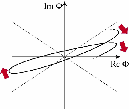
Figure 2: This figure illustrates how the AD field behaves after the beginning of the oscillation, when it is trapped by the negative thermal log potential. The thick solid line is the orbit of the AD field. The dashed lines represent the hills of the A-term, and the AD field oscillates in the valley surrounded by them. At each oscillation, it is kicked into the direction shown as the broad arrow.

The usual picture outlined above does not apply to the case when the AD field is trapped by the negative thermal log potential. First we assume the existence of the Hubble-induced A-term, and see how it spoils the baryogenesis. The relations among the mass scales, $M_{\phi}$, $M_{\theta}$ and $H$, are then $M_{\phi}\sim M_{\theta}\sim H$ before the trapping due to the thermal effect. Once the AD field is trapped by the negative thermal log potential, its amplitude, $\phi\sim(f_{(2)}^{2}T^{2}M^{n-3})^{1/(n-1)}$, decreases relatively slowly. While both $M_{\phi}$ and $M_{\theta}$ are decreasing functions of slowly varying $\phi$, the Hubble parameter diminishes faster. Thus, $M_{\phi}\gtrsim M_{\theta}\gg H$ holds until the trap ends. Since the mass scale of $\theta$ is larger than the Hubble parameter, $\theta$ starts oscillating around its minimum which is determined by the superposition of $V_{A}$ and $V_{AH}$, as soon as the AD field is trapped. During the trap, the amplitude of the oscillation of $\theta$ decreases continuously , so that $\theta$ stays very close to the bottom of the valley of the A-term when $\phi$ starts an oscillation. Therefore the AD field rotates the orbit with very large oblateness, as shown schematically in Fig. 2. It should be noted that the amplitude of the oscillation of $\phi$ remains almost constant due to the small Hubble parameter, which has a decisive influence on the evolution of the baryon number density. In order to follow the evolution of $n_{B}$, we estimate the third term in Eq. (42), which is now given as

$$q\frac{\partial V}{\partial\theta} \sim qM_{\theta}^{2}\phi^{2}=\dot{\theta}^{-1}M_{\theta}^{2}n_{B},$$ (45)

$$\lesssim M_{\theta}n_{B}\,,$$

where the last equality holds at the end point of each oscillation. Therefore the baryon number density continues to be generated around the end point, since $M_{\theta}\gg H$. Put simply, the valleys of the A-term become effectively deeper due to the enduring trap, which causes the intermittent generation of the baryon number.

Consider now the implication of the Q-ball formation. The AD field experiences instabilities when it oscillates in the $V_{gauge}$ dominated potential, and deforms into the gauge-mediation type Q balls. Since the growth rate of the instability is of the order of $M_{\phi}\sim M_{F}^{2}/\phi_{osc}$ Kasuya3 , Q balls are formed soon after the AD field starts a radial oscillation . The most important part of this argument is that the baryon number is not fixed during the process toward the Q-ball formation. When the fluctuation becomes comparable to the homogeneous mode, the system goes into the nonlinear stage, and the AD field is kicked back and forth at random in the phase direction by the A-term. It is not until Q balls are formed that the baryon number is fixed. The reason is as follows. It is known that Q balls absorb almost all the baryon number. Inside Q balls, the AD field rotates a circular orbit, so the average of the third term in Eq. (42) over a round of the orbit vanishes:

$$\oint_{0}^{2\pi}d\theta\frac{\partial V}{\partial\theta}=0,$$ (46)

which means the baryon number is fixed. Since the baryon number evolves indiscriminately until the Q-ball formation is completed, the resultant baryon asymmetry is affected by the highly nonlinear physics of the Q-ball formation. In rough estimate, the created baryon number before the system goes into the nonlinear stage is

$$n_{B}^{(i)}\simeq\frac{c_{1}}{M_{\phi}}M_{\theta}^{2}\phi_{osc}^{2}\sin{n\theta_{osc}},$$ (47)

where $\theta_{osc}(\ll 1)$ is the phase amplitude at the start of the radial oscillation, and $c_{1}M_{\phi}^{-1}$ with $c_{1}\sim\log{(\phi/\delta\phi)}=O(10)$ is the time for the fluctuation to become nonlinear. When the fluctuation of the phase becomes large, i.e., $\delta\theta/\theta\sim O(1)$, the AD field moves beyond the potential hill in the phase direction and the baryon number production restarts with random phase, $\theta_{i}({\bf x})\sim O(1)$. Here $\theta_{i}$ depends on the position ${\bf x}$. Hence this process induces the fluctuation of the baryon number density, and it takes place over and over again until Q-ball formation is completed. If the process lasted eternally, however large the baryon asymmetry is, it would be completely erased due to the baryon number violating process in equilibrium. Note that the baryon number is odd under the CPT transformation. In fact, this process is effective for a finite time, so that the only finite baryon asymmetry is annihilated. We can estimate the magnitude of the baryon asymmetry, which is erased due to the Q-ball formation processes, by calculating the typical value of the fluctuation of the baryon number density :

$$\delta n_{B}({\bf x}) \simeq \frac{1}{M_{\phi}}M_{\theta}^{2}\phi_{osc}^{2}\sum_{i}^{c_{2}}\sin{n\theta_{i}({\bf x})},$$ (48)

$$\sim \pm\frac{\sqrt{c_{2}}}{M_{\phi}}M_{\theta}^{2}\phi_{osc}^{2},$$

where $c_{2}\sim O(10)$ is the number of the restarts, and the contribution of the random phase $\theta_{i}$ is evaluated as random walk with $c_{2}$ steps in the second line. Since $\theta_{osc}\ll 1$ in the present situation, we have $n_{B}^{(i)}\ll\delta n_{B}$, which means that $n_{B}$ is dominated by the fluctuation due to the Q-ball formation process. Moreover, the dynamics is chaotic in the sense that a tiny change results in a quite different baryon number. Thus, the baryon asymmetry generated during the homogeneous evolution is swallowed up in the large fluctuation, leading to the baryon symmetric universe.

We performed the numerical simulation in order to confirm whether the baryon asymmetry is really determined through the Q-ball formation. For the numerical calculation, we take the variables dimensionless as follows.

$$\varphi = \frac{\Phi}{M_{S}},$$

$$\tau = \frac{M_{F}^{2}}{M_{S}}t,$$

$$\chi_{i} = \frac{M_{F}^{2}}{M_{S}}x_{i},$$ (49)

The initial conditions of the homogeneous parts are taken as

$${\rm Re}\left[\varphi(0)\right] = 1.0\times 10^{2},$$

$${\rm Im}\left[\varphi(0)\right] = 1.0\times 10^{-3},$$

$$\varphi^{\prime}(0) = 0.0,$$ (50)

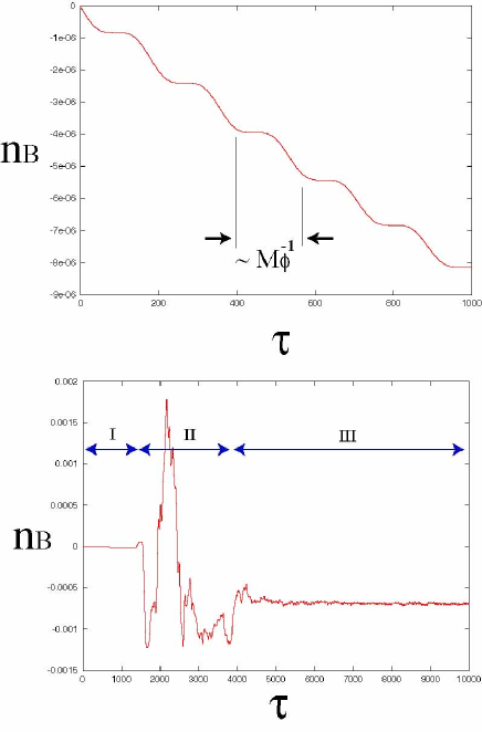
Figure 3: The evolution of the baryon number during Q-ball formation is shown. As shown in the lower figure, it can be classified into three parts. First the AD field is kicked around the endpoint at each oscillation (see Fig. 2), leading to the intermittent baryogenesis (interval I). Then the behavior of the baryon number becomes chaotic, as the fluctuations grows (interval II). Finally, it is fixed after the Q-ball formation is completed. The upper figure is the blowup of the evolution for the baryon number during the interval I.

where the prime denotes the derivative with respect to $\tau$, and we redefined the phase of the AD field so that the real direction coincides with one of the valleys of the A-term with the mass scale $M_{\theta}/M_{\phi}=10^{-1.8}$. Taking account of fluctuations which originate from the quantum fluctuations, we give $\varphi$ fluctuations with amplitudes $10^{-7}$ times smaller than the homogeneous mode. We have confirmed that the smaller fluctuations just delay the formation of Q balls. For simplicity we neglected the cosmic expansion. The results are shown in Fig. 3. It shows that the baryon number is generated at the end point of each oscillation for some time $\sim c_{1}M_{\phi}^{-1}$, but it soon goes into the chaotic phase until the Q-ball formation is completed. If we change the initial seed for the fluctuation, it is probable that the resultant baryon asymmetry inside the box of the lattices becomes positive. The reason why the resultant baryon number takes nonzero value is that the size of the box under consideration is finite. If the same calculation were done with the infinitely large box, the resultant baryon number would be exactly zero.

Lastly we comment on the case without the Hubble-induced A-term. Now $M_{\phi}>H>M_{\theta}$ at the onset of the oscillation can be realized since the mass scale of $\theta$ is smaller than that in the previous case. Then the initial phase amplitude $\theta_{osc}$ is comparable to the random phase $\theta_{i}$, hence the net baryon number can be nonzero. In the next section we estimate the resultant baryon asymmetry in this case, taking account of the Q-ball formation.

IV Baryogenesis

As we have shown in the previous section, the Hubble-induced A-term spoils the baryogenesis through the Q-ball formation. On the other hand, if it were not for the Hubble-induced A-term, we can avoid this problem since $M_{\phi}>H>M_{\theta}$ at the beginning of the oscillation is possible. Then the baryon number just before the Q-ball formation is completed is roughly estimated as

$$n_{B}^{(f)}\sim\frac{c_{1}}{M_{\phi}}M_{\theta}^{2}\phi_{osc}^{2}>\frac{\sqrt{c_{2}}}{M_{\phi}}M_{\theta}^{2}\phi_{osc}^{2},$$ (51)

where $c_{1}\sim c_{2}\sim O(10)$, and we used $\theta_{osc}\sim O(1)$ in the present case. Thus we expect that the finite baryon asymmetry remains even if the AD field gets randomly kicked in the phase direction during the nonlinear stage. In other words, the resultant baryon number is almost determined due to the dynamics before the AD field goes into the nonlinear phase, so subsequent Q-ball formation does not affect the baryon asymmetry.

To satisfy the requirement that the net baryon number is generated, the following condition must be satisfied:

$$M_{\theta}<H_{osc},$$ (52)

where

$$M_{\theta} \simeq \sqrt{\frac{m_{3/2}\phi_{osc}^{n-2}}{M^{n-3}}},$$ (53)

$$H_{osc} \simeq \left\{\begin{array}[]{ll}\displaystyle{\frac{T_{osc}^{4}}{T_{RH}^{2}M_{G}}}&{\rm for~{}~{}}T_{osc}>T_{RH},\\ &\\ \displaystyle{\frac{T_{osc}^{2}}{M_{G}}}&{\rm for~{}~{}}T_{osc}<T_{RH}.\end{array}\right.$$ (57)

Then the baryon number is generated as

$$n_{B}(t_{osc})\simeq\frac{1}{M_{\phi}}\frac{m_{3/2}\phi_{osc}^{n}}{M^{n-3}}\,,$$ (58)

where it should be noted that $M_{\phi}=M_{F}^{2}/\phi_{osc}$ is used instead of the Hubble parameter, because the kick due to the A-term lasts for $\delta t\sim M_{\phi}^{-1}$, and we also set the numerical factor to be unity. The almost all baryon number is absorbed into the subsequently formed Q balls with the typical charge given as Eq. (12) . Hereafter we consider the two cases, depending on whether the Q balls dominate the universe or not. If the Q balls dominates the universe, they must be unstable and decay before the epoch of big bang nucleosynthesis (BBN). Thus, the mass per unit charge and the decay temperature are constrained as

$$M_{F}Q^{-\frac{1}{4}} > 1{\rm GeV},$$ (59)

$$T_{d}=\left(\frac{\pi^{2}g_{*}}{90}\right)^{-\frac{1}{4}}\sqrt{\frac{M_{F}M_{G}}{48\pi Q^{\frac{5}{4}}}} > 10{\rm MeV}.$$ (60)

Since the universe is reheated again, the gravitino problem is alleviated in this case. Accordingly the constraints Eqs.(III) and (III) with $\gamma$ given as Eq. (III) are adopted. The baryon-to-entropy ratio is given as

$$\frac{n_{B}}{s} = \frac{3}{4}\frac{n_{B}(t_{osc})T_{d}}{M_{F}^{4}},$$ (64)

$$\sim \left\{\begin{array}[]{ll}\displaystyle{30\times\left(\frac{g_{*}}{10}\right)^{-\frac{1}{4}}m_{3/2}^{-n+\frac{5}{2}}M_{F}^{2(n-3)}M^{-(n-3)}M_{G}^{\frac{1}{2}}}&{\rm for~{}~{}}\displaystyle{m_{3/2}>\left(M_{F}^{2n-4}M^{-(n-3)}\right)^{\frac{1}{n-1}}},\\ &\\ \displaystyle{30\times\left(\frac{g_{*}}{10}\right)^{-\frac{1}{4}}m_{3/2}M_{F}^{-\frac{n}{n-1}}M^{-\frac{(n-3)}{2(n-1)}}M_{G}^{\frac{1}{2}}}&{\rm for~{}~{}}\displaystyle{m_{3/2}<\left(M_{F}^{2n-4}M^{-(n-3)}\right)^{\frac{1}{n-1}}},\end{array}\right.$$

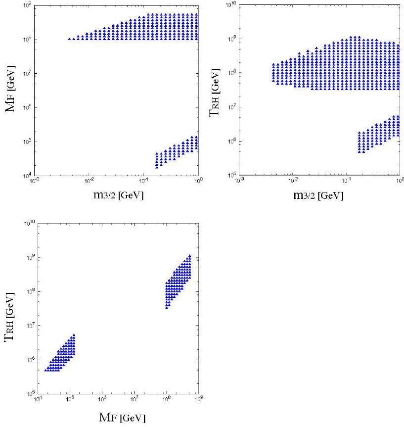
Figure 4: The allowed regions for $m_{3/2}$, $M_{F}$ and $T_{RH}$ in the case that the Q balls dominate the universe are shown. Here we set $f_{(1)}=f_{(2)}=0.3$, $M=M_{G}$ and $n=6$.

The allowed regions for $m_{3/2}$, $M_{F}$ and $T_{RH}$ satisfying the above constraints are shown in Fig.4 and 5, where we set $f_{(1)}=f_{(2)}=0.3$, $M=M_{G}$ and $n=6$. It shows that the baryon-to-entropy ratio can be large enough to explain the present asymmetry. For instance, it takes the value as

$$\frac{n_{B}}{s}=6\times 10^{-7}\left(\frac{g_{*}}{10}\right)^{-\frac{1}{4}}\left(\frac{m_{3/2}}{100{\rm MeV}}\right)\left(\frac{M_{F}}{5\times 10^{8}{\rm GeV}}\right)^{-\frac{6}{5}}\left(\frac{M}{M_{G}}\right)^{-\frac{3}{10}},$$ (65)

where $m_{3/2}$ and $M_{F}$ is assumed to satisfy all the constraints stated above, so their values must be included in the allowed regions shown in Fig.4 and 5. Though the above value is a little larger compared to the expected one $\sim 10^{-10}$, it might be suppressed by the unknown CP phase $\theta_{osc}$which we assume to be of the order of unity here. Although $M>M_{G}$ is possible since the definition of $M$ in Eq. (3) includes a possibly small coupling constant, it does not work to take larger $M$. This is because the requirement that Q balls decay before the BBN sets the lower bound for $M_{F}$ which is a positive power of $M$, so the allowed regions shown in Fig.4 and 5 would disappear for $M\gg M_{G}$.

Next we consider the case that the energy of Q balls is subdominant before the BBN. If Q balls are unstable, they must decay before the BBN, otherwise their decay product might destroy the light elements and spoil the success of the BBN. If Q balls are stable, the resultant baryon asymmetry is suppressed by $\Delta Q/Q$, where $\Delta Q$ is the evaporated charge. Also the abundance of remnant Q balls are constrained in order not to overclose the universe. Namely,

$$\Omega_{Q}=\frac{M_{F}Q^{-1/4}}{m_{n}}\frac{\Omega_{B}}{\varepsilon}\frac{Q}{\Delta Q}<1,$$ (66)

where $m_{n}$ is the nucleon mass, and $\Omega_{Q(B)}$ is the ratio of the energy density of Q balls (or baryon) to the critical density. The baryon-to-entropy ratio is expressed as

$$\frac{n_{B}}{s}\simeq\left(\frac{45}{2\pi^{2}g_{*}}\right)\frac{n_{B}(t_{osc})}{T_{osc}^{3}}\times\kappa_{1}\times\kappa_{2},$$ (67)

where

$$\kappa_{1} \equiv \left\{\begin{array}[]{ll}1&{\rm~{}~{}~{}~{}~{}for~{}~{}}T_{osc}<T_{RH},\\ &\\ T_{RH}^{5}/T_{osc}^{5}&{\rm~{}~{}~{}~{}~{}for~{}~{}}T_{osc}>T_{RH},\end{array}\right.$$ (71)

$$\kappa_{2} \equiv \left\{\begin{array}[]{ll}1&{\rm~{}~{}~{}~{}~{}for~{}~{}unstable~{}~{}Q~{}~{}balls},\\ &\\ \Delta Q/Q&{\rm~{}~{}~{}~{}~{}for~{}~{}stable~{}~{}Q~{}~{}balls}.\end{array}\right.$$ (75)

Since the reheating temperature is now constrained by the gravitino problem, the constraints Eqs.(III) and (III) with $\gamma=1$ are adopted. The allowed regions for $m_{3/2}$, $M_{F}$ and $T_{RH}$ satisfying the above constraints are shown in Fig.6 and 7, where we set $f_{(1)}=f_{(2)}=0.3$, $M=M_{G}$ and $n=6$. It shows that the baryon-to-entropy ratio can be as large as $\sim 10^{-12}$, which is a little smaller than the favored value $\sim 10^{-10}$. However, it can be cured by taking smaller $M$, the GUT scale for instance. Fig.8 and 9 represent the allowed regions for $m_{3/2}$, $M_{F}$ and $T_{RH}$ in the case of $f_{(1)}=f_{(2)}=0.3$, $M=10^{16}$ GeV and $n=6$. It shows that the baryon-to-entropy ratio can be now as large as $10^{-10}$ for unstable Q balls, although it is too small to explain the present asymmetry for stable Q balls. For instance, it is given as

$$\frac{n_{B}}{s}\sim 3\times 10^{-11}\left(\frac{g_{*}}{200}\right)^{-1}\left(\frac{m_{3/2}}{100{\rm MeV}}\right)\left(\frac{M_{F}}{2\times 10^{7}{\rm GeV}}\right)^{-\frac{36}{5}}\left(\frac{T_{RH}}{10^{6}{\rm GeV}}\right)^{5}\left(\frac{M}{10^{16}{\rm GeV}}\right)^{\frac{6}{5}},$$ (76)

for unstable Q balls.

V Conclusion

We have studied whether the AD baryogenesis works in the gauge-mediated SUSY breaking models, if the AD field is trapped by the negative thermal log potential which is known to be ubiquitous in the MSSM. The most striking feature is that the Hubble parameter becomes much smaller than the mass scale of the radial component of the AD field, during the trap. Then, the amplitude of the AD field decreases so slowly that the baryon number is not fixed even after the onset of radial oscillation. A further important point is that the AD field experiences spatial instabilities and deforms into Q balls. Therefore the baryon asymmetry can be washed out due to the random kick in the phase direction during the process of Q-ball formation. Indeed, it has been shown that the net baryon number vanishes if the Hubble parameter is smaller than the mass scale of phase direction, since the randomly generated baryon number surpasses the baryon number just before the nonlinear stage begins. This is always the case if the Hubble-induced A-term exists. Also we confirmed the chaotic behavior of the baryon number with use of numerical calculation. However, the Hubble-induced A-term does not necessarily exist. In fact, we have found that it is possible to generate the right amount of the baryon asymmetry in the absence of the Hubble-induced A-term, if the Q balls are unstable. Thus, it should be emphasized that the AD baryogenesis is still a viable candidate, even if both the thermal effect and Q-ball formation are fully taken into account.

ACKNOWLEDGMENTS

F.T. thanks Masahide Yamaguchi for useful discussion and comments.

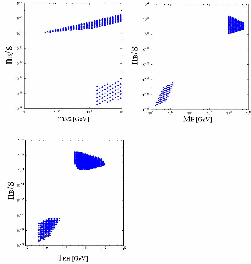
Figure 5: The baryon-to-entropy ratio is plotted for the allowed regions in Fig. 4.

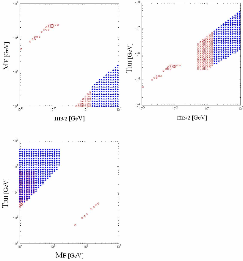
Figure 6: The allowed regions for $m_{3/2}$, $M_{F}$ and $T_{RH}$ in the case that the Q balls do not dominate the universe are shown. Here we set $f_{(1)}=f_{(2)}=0.3$, $M=M_{G}$ and $n=6$. The open cicle and closed triangle denote stable and unstable Q balls respectively.

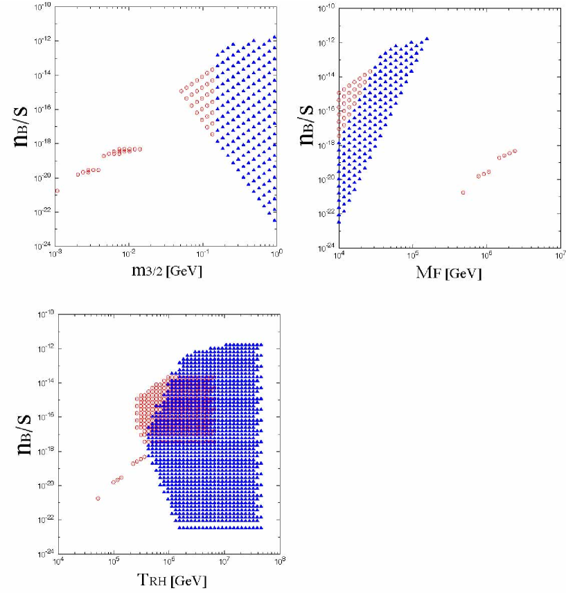
Figure 7: The baryon-to-entropy ratio is plotted for the allowed regions in Fig. 6. The open cicle and closed triangle denote stable and unstable Q balls respectively.

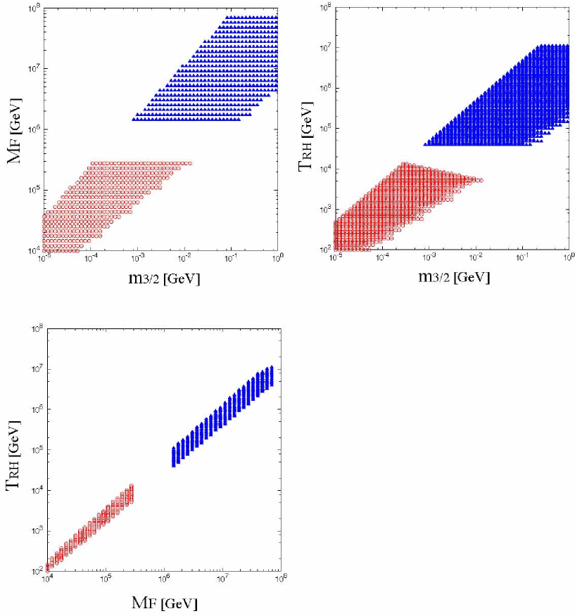
Figure 8: The allowed regions for $m_{3/2}$, $M_{F}$ and $T_{RH}$ in the case that the Q balls do not dominate the universe are shown. Here we set $f_{(1)}=f_{(2)}=0.3$, $M=10^{16}$ GeV and $n=6$. The open cicle and closed triangle denote stable and unstable Q balls respectively.

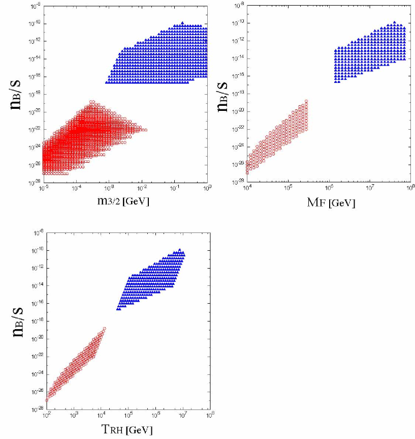
Figure 9: The baryon-to-entropy ratio is plotted for the allowed regions in Fig. 8. The open cicle and closed triangle denote stable and unstable Q balls respectively.

References

- (1)
- (2) I. Affleck and M. Dine, Nucl. Phys. B249, 361 (1985).
- (3) M. Dine, L. Randall, and S. Thomas, Nucl. Phys. B458, 291 (1996).
- (4) R. Allahverdi, B. A. Campbell, and J. Ellis, Nucl. Phys. B579, 355 (2000).
- (5) A. Anisimov and M. Dine, Nucl. Phys. B619, 729 (2001).
- (6) A. Kusenko and M. Shaposhnikov, Phys. Lett. B 418, 46 (1998).
- (7) K. Enqvist and J. McDonald, Nucl. Phys. B538, 321 (1999).
- (8) S. Kasuya and M. Kawasaki, Phys. Rev. D 61, 041301 (2000).
- (9) For a review, see, e.g. G.F. Giudice and R. Rattazzi, Phys. Rep. 322, 419 (1999).
- (10) S. Kasuya and M. Kawasaki, Phys. Rev. Lett. 85, 2677 (2000).
- (11) S. Kasuya and M. Kawasaki, Phys. Rev. D 64, 123515 (2001).
- (12) A. de Gouvêa, T. Moroi, and H. Murayama, Phys. Rev. D 56, 1281 (1997).
- (13) K. Enqvist and J. McDonald, Phys. Lett. B 425, 309 (1998).
- (14) T. Asaka, M. Fujii, K. Hamaguchi, and T. Yanagida, Phys. Rev. D 62, 123514 (2000).
- (15) T. Asaka, M. Fujii, K. Hamaguchi, and T. Yanagida, Phys. Rev. D 63, 123513 (2001).
- (16) G. Dvali, A. Kusenko, and M. Shaposhnikov, Phys. Lett. B 417, 99 (1998).
- (17) A. Cohen, S. Coleman, H. Georgei, and A. Manohar, Nucl. Phys. B272, 301 (1986).
- (18) M. Laine, and M. Shaposhnikov, Nucl. Phys. B532, 376 (1998).
- (19) R. Banerjee and K. Jedamzik, Phys. Lett. B 484, 278 (2000).
- (20) D. Lyth and A. Riotto, Phys. Rep. 314, 1 (1999).