Adiabatic potentials and spectra of heavy hybrid mesons

Abstract

Using the QCD string approach the adiabatic potentials and spectra of $b\bar{b}$-hybrid mesons are calculated. The results are compared to lattice studies.

1. An assumption about existence of the hybrid mesons consisting of valence quark and antiquark and valence gluon was made for the first time by Okun and Vainshtein [1] just afterwards the QCD appeared. Last decade was a time of intensive studies of hybrid mesons both in experimental and in theoretical frameworks.

In this report we study the system of static quark and antiquark and dynamical gluon joined to the formers by the infinitely thin string of background gluon field in analytic QCD string approach [2], [3] based on the background perturbation theory [4]. In other words, we study spectrum of the vibrations of the confining string, or spectrum of the adiabatic potentials. We will pay our attention to the small and intermediate quark-antiquark separations, which are directly related to the spectrum of heavy hybrid mesons. Using the adiabatic potentials, we will calculate spectra of $b\bar{b}$-hybrid mesons.

2. In the framework of the background perturbation theory we start from the propagator of the valence gluon in the background field $B$ [4],

$$G_{\mu\nu}=(D^{2}(B)\,\delta_{\mu\nu}+2igF_{\mu\nu}(B))^{-1},$$ (1)

where $D(B)$ is the covariant derivative depending on the field $B$; $F_{\mu\nu}(B)$ is the background field strength tensor, which is related to the spin effects and will be considered below. In the formalism of the Fock-Feynman-Shwinger representation the Green function of the hybrid meson with the static quark and antiquark reduces to the form (see [3] and references therein)

$$G_{h}(\bar{X},X)=\int^{\infty}_{0}ds\int({\cal D}z_{g})_{x_{g}y_{g}}\exp(-K)\langle{\cal W}_{h}\rangle_{B},$$ (2)

where ${\cal W}_{h}$ is the Wilson loop of the hybrid meson, consisting of the trajectories $\Gamma_{Q}$, $\Gamma_{\bar{Q}}$ and $\Gamma_{g}$ of valence quark, antiquark and gluon (see Fig. 1), and $K$ is the kinetic energy of the gluon.

Figure 1: Wilson loop of hybrid meson

In what follows we will use the area law for the Wilson loop, which is confirmed by the lattice QCD, see e.g. [5]. The area law for hybrid mesons takes the form

$$\langle{\cal W}_{h}\rangle_{B}=\frac{N_{c}^{2}-1}{2}\exp(-\sigma(S_{1}+S_{2})),$$ (3)

where $S_{1}~{}(S_{2})$ is an area of the minimal surface bounded by the trajectores of valence quark (antiquark) and gluon. We parametrise the minimal surfaces introducing parameters $0\leq\tau\leq T$ and $0\leq\beta_{1,2}\leq 1$. It is also convenient to introduce einbein fields $\mu(\tau),~{}\nu_{1,2}(\tau,\beta)$ and write the Green function of the hybrid meson in the form

$$G_{h}(\bar{X},X)=\int({\cal D}^{3}z_{g})_{x_{g}y_{g}}{\cal D}\mu\,{\cal D}\nu_{1}\,{\cal D}\nu_{2}\exp\left(-\int_{0}^{T}d\tau\,L\right),$$ (4)

which defines the following string Hamiltonian [3],

$$H={\mbox{\boldmath${\rm p}$}}\,\dot{\mbox{\boldmath${\rm r}$}}-L=H_{0}+\frac{\mu}{2}+\int^{1}_{0}d\beta_{1}\,\frac{\sigma^{2}r^{2}_{1}}{2\nu_{1}}+\int^{1}_{0}d\beta_{2}\,\frac{\sigma^{2}r^{2}_{2}}{2\nu_{2}}+\int^{1}_{0}d\beta_{1}\,\frac{\nu_{1}}{2}+\int^{1}_{0}d\beta_{2}\,\frac{\nu_{2}}{2},$$ (5)

where

$$H_{0}=\frac{p^{2}}{2(\mu+J_{1}+J_{2})}+\frac{1}{2\Delta(\mu+J_{1}+J_{2})}\times$$

$$\times\left\{\frac{(\mbox{\boldmath${\rm p}$}\,\mbox{\boldmath${\rm r}$}_{1})^{2}}{r^{2}_{1}}J_{1}(\mu+J_{1})+\frac{(\mbox{\boldmath${\rm p}$}\,\mbox{\boldmath${\rm r}$}_{2})^{2}}{r^{2}_{2}}J_{2}(\mu+J_{2})+\frac{2J_{1}J_{2}}{r^{2}_{1}r^{2}_{2}}(\mbox{\boldmath${\rm r}$}_{1}\mbox{\boldmath${\rm r}$}_{2})(\mbox{\boldmath${\rm p}$}\,\mbox{\boldmath${\rm r}$}_{1})(\mbox{\boldmath${\rm p}$}\,\mbox{\boldmath${\rm r}$}_{2})\right\},$$ (6)

$$\Delta=(\mu+J_{1})(\mu+J_{2})-J_{1}J_{2}\frac{(\mbox{\boldmath${\rm r}$}_{1}\mbox{\boldmath${\rm r}$}_{2})^{2}}{r^{2}_{1}r^{2}_{2}},~{}~{}J_{i}=\int^{1}_{0}d\beta_{i}\,\beta_{i}^{2}\nu_{i}(\beta_{i}),~{}~{}i=1,2,$$

${\rm r}$ and ${\rm p}$ are the coordinate and momentum of the valence gluon, $\mbox{\boldmath${\rm r}$}_{1,2}=\mbox{\boldmath${\rm r}$}\pm\mbox{\boldmath${\rm R}$}/2$, where $\pm\mbox{\boldmath${\rm R}$}/2$ are locations of the static quark and antiquark. Einbein fields are to be excluded from the Hamiltonian by the conditions

$$\frac{\partial H}{\partial\mu}=0,~{}~{}\frac{\delta H}{\delta\nu_{i}(\beta_{i})}=0.$$ (7)

One can show that einbein $\mu$ plays the role of the constituent mass of the gluon, $\nu_{i}(\beta)$ the energy density of the background field along the string, and $J_{i}$ the inertia of the string.

3. Proceed now to the calculations of the spectrum of the string Hamiltonian at small and intermediate quark-antiquark separations, $R\mathrel{\mathchoice{\lower 3.6pt\vbox{\halign{$\mathsurround=0pt\displaystyle\hfil#\hfil$\cr<\crcr\sim\crcr}}}{\lower 3.6pt\vbox{\halign{$\mathsurround=0pt\textstyle\hfil#\hfil$\cr<\crcr\sim\crcr}}}{\lower 3.6pt\vbox{\halign{$\mathsurround=0pt\scriptstyle\hfil#\hfil$\cr<\crcr\sim\crcr}}}{\lower 3.6pt\vbox{\halign{$\mathsurround=0pt\scriptscriptstyle\hfil#\hfil$\cr<\crcr\sim\crcr}}}}1$ fm. In this region the inertia of the string $J_{i}$ is much smaller than the constituent mass of the gluon, $J_{i}\ll\mu$. Neglecting $J_{i}$ and calculating extremum over $\mu$ in the initial Hamiltonian, we arrive at the Hamiltonian of the potential model,

$$H=\sqrt{\mbox{\boldmath${\rm p}$}^{2}}+\sigma r_{1}+\sigma r_{2}.$$ (8)

However, it is more convenient to calculate the eigenvalues $E(\mu)$ of the Hamiltonian keeping the einbein $\mu$, and then minimize them with respect to the einbein,

$$\frac{\partial E(\mu)}{\partial\mu}=0.$$ (9)

This procedure is of common use in the QCD string approach, and, for the ordinary mesons, is justified with the accuracy better than 5% (see e.g. [2]).

Besides the nonperturbative string part considered above, the hybrid Hamiltonian should contain the perturbative one $V_{c}$, which is dominated by the one-gluon exchange,

$$V_{c}=-\frac{3\,\alpha_{s}}{2r_{1}}-\frac{3\,\alpha_{s}}{2r_{2}}+\frac{\alpha_{s}}{6R}.$$ (10)

Therefore, the Hamiltonian with the string inertia neglected takes the form

$$H=\frac{\mu}{2}+\frac{p^{2}}{2\mu}+\sigma r_{1}+\sigma r_{2}+V_{c}.$$ (11)

Despite its nonrelativistic appearance, this Hamiltonian is essentially relativistic due to condition (9).

The Hamiltonian of the string correction of the order of $J/\mu$ derived from (5), (6) has transparent form,

$$H^{\mathrm{string}}=-\frac{\sigma}{6\mu^{2}}\left(\frac{1}{r_{1}}L_{1}^{2}+\frac{1}{r_{2}}L_{2}^{2}\right),$$ (12)

where $\mbox{\boldmath${\rm L}$}_{i}=\mbox{\boldmath${\rm r}$}_{i}\times\mbox{\boldmath${\rm p}$}$.

Spin interaction in ordinary mesons with heavy quarks of mass $m$ have been expressed through the number of universal uknown potentials of order $1/m^{2}$ using the Wilson loop in [6]. In the framework of QCD string approach these potentials were calculated using the method of field correlators, see [2] and references therein. The role of the mass $m$ is performed in the approach by the einbein $\mu$, and the results therefore are applicable to both light and heavy quarks.

Spin interaction of the valence gluon with the quark and antiquark in hybrid mesons is generated by the strength tensor term in propagator (1), which can be rewritten as $F_{ik}=i(\mbox{\boldmath${\rm S}$}\mbox{\boldmath${\rm B}$})_{ik}$, where the spin operator ${\rm S}$ acts onto the gluon wave function ${\rm\Psi}$ according to $\left(S_{i}\mbox{\boldmath${\rm\Psi}$}\right)_{j}=-i\epsilon_{ijk}\Psi_{k}$. Performing calculations similar to ones of [2], we derive the following relations in Eichten-Feinberg notations,

$$V_{1}^{\mathrm{(p)}}=0,~{}~{}V_{2}^{\mathrm{(p)}}=\epsilon^{\mathrm{(p)}},\quad\mbox{ where }\quad\epsilon^{\mathrm{(p)}}=-\frac{3\alpha_{s}}{2r_{i}},~{}~{}i=1,2,$$ (13)

and

$$V_{1}^{\mathrm{(np)}}=-\epsilon^{\mathrm{(np)}},~{}~{}V_{2}^{\mathrm{(np)}}=0,\quad\mbox{ where }\quad\epsilon^{\mathrm{(np)}}=\sigma r_{i}.$$ (14)

One can verify that the Gromes relation $\epsilon+V_{1}-V_{2}=0$ is justified for both perturbative and nonperturbative potentials. The corresponding Hamiltonian consists of the following perturbative and nonperturbative parts [3],

$$H^{\mathrm{LS}\,\mathrm{(p)}}=\frac{3\alpha_{s}}{4\mu^{2}}\left(\frac{\mbox{\boldmath${\rm L}$}_{1}\mbox{\boldmath${\rm S}$}}{r_{1}^{3}}+\frac{\mbox{\boldmath${\rm L}$}_{2}\mbox{\boldmath${\rm S}$}}{r_{2}^{3}}\right),$$ (15)

$$H^{\mathrm{LS}\,\mathrm{(np)}}=-\frac{\sigma}{2\mu^{2}}\left(\frac{\mbox{\boldmath${\rm L}$}_{1}\mbox{\boldmath${\rm S}$}}{r_{1}}+\frac{\mbox{\boldmath${\rm L}$}_{2}\mbox{\boldmath${\rm S}$}}{r_{2}}\right).$$ (16)

We calculate the energy levels of the initial Hamiltonian (11) variationally, using the Gaussian wave functions of the gluon,

$$\vec{\Psi}_{jl\Lambda}(\mbox{\boldmath${\rm r}$})=\phi_{l}(r)\sum_{\mu_{1}\mu_{2}}C^{j\Lambda}_{l\mu_{1}l\mu_{2}}Y_{l\mu_{1}}\left(\frac{\mbox{\boldmath${\rm r}$}}{r}\right)\vec{\chi}_{1\mu_{2}},$$ (17)

$$\phi_{l}(r)\sim\exp\left(-\beta^{2}r^{2}/2\right).$$

The corrections (12)-(16) amount to the decrease of the total energy about 70-150 MeV depending on the level.

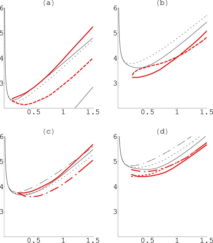
Figure 2: Hybrid potentials with corrections included (black curves) compared to lattice ones (color curves) in units $1/r_{0}=$ 400 MeV ($r_{0}=2.5$ GeV^-1). $Q\bar{Q}$-distance $R$ is measured in $2r_{0}\approx$ 1 fm. States (a)–(d) are given in Table 1. Solid, dashed and dashed-dotted curves correspond to $\Lambda=0,1$ and 2. Solid line at right bottom corner of Fig.2(a) represents the Coulomb+linear potential with $\alpha_{s}=0.4$ and $\sigma=0.21$ GeV².

(a)	$\Sigma_{u}^{-},~{}\Pi_{u}$
(b)	$\Sigma_{g}^{+},~{}\Pi_{g}$
(c)	$\Sigma_{g}^{-},~{}\Pi_{g},~{}\Delta_{g}$
(d)	$\Sigma_{u}^{+},~{}\Pi_{u},~{}\Delta_{u}$

Table 1: Quantum numbers of adiabatic levels of Fig. 2

In Fig. 2 the resulting adiabatic potential energy levels are shown in comparison with the lattice results [7]. Quantum numbers of the levels in the diatomic molecule notations are given in Table 1. The potentials are normalized to the ground $Q\bar{Q}$-level shown in the right bottom corner of Fig. 2(a). We can see overall correspondence with the lattice. The curves tend to form three multiplets with different values of the gluon angular momentum. This is a confirmation that the angular moment of the gluon is a good quantum number. When $R$ goes to zero, the potentials increase rapidly due to the Coulomb repulsion of quark and antiquark in octet state of color $SU(3)$. Note the wrong bend of $\Pi_{g}$ lattice level in Fig. 2(b) and absence of $\Pi_{g}$ lattice level in Fig. 2(c), which clearly means that these two $\Pi_{g}$ levels are not properly resolved on the lattice. The order of levels in our approach correspond to the lattice one, with the exception of Fig. 2(c). Different separations between the levels of Fig. 2(a) in our and lattice approaches is presumably related to the influence of the Coulomb gluon-quark and gluon-antiquark interaction on the gluon wave function. Variational calculations using the Coulomb-modified wave functions are needed to verify this assumption, which will be performed in future publications.

Lowest level with the quantum numbers $\Sigma^{-}_{g},~{}\Pi_{g}$ is absent on the lattice and therefore not shown in Fig. 2. Comparative analysis of adiabatic potentials of other approaches can be found in [3].

4. Let us calculate spectra of masses of the heavy hybrid mesons in Born-Oppenheimer approximation assuming that the motion of the valence quark and antiquark is slow compared to the motion of the valence gluon and using the adiabatic potentials. In this case an essential region is the one near the minimum of the potential, where the adiabatic potential can be replaced by the oscillatory one. Therefore the problem reduces to the calculation of the spectrum of three-dimentional oscillator.

We tune the values of parameters $\alpha_{s}=0.225$, $\sigma=0.18$ GeV², $m_{b}=4.56$ GeV to reproduce the experimental value of the ground state of $b\bar{b}$-meson, $M^{\Upsilon(1S)}_{\mathrm{exp}}=9.4$ GeV, from the Cornell potential,

$$V^{b\bar{b}}=2m_{b}-\frac{4}{3}\frac{\alpha_{s}}{R}+\sigma R.$$ (18)

Then we calculate the masses of $b\bar{b}$ hybrid mesons through the equation

$$M^{b\bar{b}g}=2m_{b}+E^{\mathrm{osc}},$$ (19)

where $E^{\mathrm{osc}}$ is the energy of $b$-quarks in the adiabatic potential, approximated in the vicinity of its minimum by the oscillatory one.

$l=1,~{}l_{Q\bar{Q}}=0$ (GE)	$M^{b\bar{b}g}=10.83\mbox{ GeV}$
$l=0,~{}l_{Q\bar{Q}}=1$ (QE)	$M^{b\bar{b}g}=10.92\mbox{ GeV}$

Table 2: The masses of the lowest $b\bar{b}$-exotic states in our approach

Lattice QCD [7]	$M^{b\bar{b}g}$=10.8 GeV
QCD string approach [8]	$M^{b\bar{b}g}$=10.64 GeV

Table 3: The masses of lowest $b\bar{b}$-exotic states with $J^{PC}=1^{-+}$ in other works

The lowest exotic hybrid states have quantum numbers $J^{PC}=1^{-+}$ and may be of two different kinds, the gluon-excited (GE) one, with the gluon angular momentum $l=1$ and quark-antiquark relative angular moment $l_{Q\bar{Q}}=0$, and quark-excited (QE) one, with $l=0$ and $l_{Q\bar{Q}}=1$. Their masses are given in Table 2. One can calculate the energy of the gluon excitation using the mass of the GE-state from the Table,

$$\Delta M=M^{b\bar{b}g}_{(GE)}-M^{\Upsilon(1S)}=1.43\mbox{ GeV}.$$ (20)

One can see that $\Delta M\ll m_{b}$ so that the adiabatic approximation for $b\bar{b}$-hybrid mesons is justified. The mass of $c$-quark is close to the energy of gluon excitation, so that adiabatic approximation for $c\bar{c}$-hybrid mesons is invalid.

The mass of the lowest exotic state of $b\bar{b}$-hybrid meson was calculated on the lattice [7], as well as in the QCD string approach in the work [8]. The results are shown in the Table 3. In lattice QCD lowest quark-excited state is absent, as it was already noted above. One can see from the Tables 2, 3 that the mass of the gluon-excited state computed in the adiabatic approximation is almost the same as ours. Note that in both cases quenched approximation was used. One can guess that a proper account of the see quarks will not change the result significantly.

The results of the work [8] were obtained using the Hamiltonian (11) and the method of einbein field. The main difference between this and ours results is due to the large constant subtracted in [8]. The adiabatic Born-Oppenheimer approximation was not used in [8] and string- and spin-corrections to Hamiltonian were not considered.

One can find recent comparison of existing calculations of lowest exotic hybrid meson masses in other models in [9]. Note that ITEP sum rules and flux-tube model predict lowest exotic $b\bar{b}$ hybrid mass with large error bars, which include both our numbers, and bag model seems to underestimate the mass. Recent calculations of GE-mode in quark-gluon model [9] are in good agreement with both lattice and our results. The mass of QE-mode in [9] is less than GE-one, unlike ours, see Table 2. This discrepency is presumably due to poor accuracy of our variational procedure for lowest adiabatic level.

In conclusion, we have shown that the QCD string approach allows to calculate the adiabatic potentials and masses of heavy hybrid mesons in a good agreement with lattice QCD. Our further tasks are use of more elaborated variational procedure for the calculation of the lowest adiabatic levels, as well as accurate calculations of hybrid spectra, wave functions and decays both within and beyond the adiabatic approximation.

This work has been supported by RFBR grants 00-02-17836, 00-15-96786, and INTAS 00-00110.

References

- [1] L.B.Okun and A.I.Vainstein, Sov.J.Nucl.Phys. 23, 716 (1976).
- [2] Yu.A.Simonov, Lectures at the XVII International School of Physics, Lisbon, 1999, hep-ph/9911237.
-
[3]
Yu.S.Kalashnikova and D.S.Kuzmenko, preprint ITEP N2
(2002), Phys.Atom.Nucl. (in press), hep-ph/0203128;
D.S.Kuzmenko, Ph.D. thesis, Moscow (2002) (in russian). - [4] Yu.A.Simonov, in: Lecture Notes in Physics, v.479 p.139 (1996), Springer-Verlag, Berlin-Heidelberg; Phys.At.Nucl. 58, 107 (1995).
- [5] A.M.Badalian, D.S.Kuzmenko, this volume, hep-ph/0302072.
-
[6]
E.Eichten, F.Feinberg, Phys.Rev. D23, 2724 (1981);
D.Gromes, Z.Phys. C26, 401 (1984). - [7] K.J.Juge, J.Kuti, and C.Morningstar, in Proc. of the Third Int. Conf. on Quark Confinement and the Hadron Spectrum, Jefferson Lab, 1998, hep-lat/9809015; in Proc. of LATTICE98, Boulder, USA, 1998, Nucl.Phys.Proc.Suppl. 73, 590 (1999).
- [8] Yu.S.Kalashnikova and Yu.B.Yufryakov, Phys.Lett. B359, 175 (1995); Phys.At.Nucl. 60, 307 (1997).
- [9] F. Iddir, L. Semlala, hep-ph/0211289.